PID CONTROL FOR ROBOTIC ARM

FINAL DEGREE PROJECT

STUDENT: MATEO UBEDA ALMERICH

COVENTRY UNIVERSITY SUPERVISOR: AAMER SALEEM

FACULTY OF ENGINEERING, ENVIRONMENT AND COMPUTING

UPV SUPERVISOR: SALVADOR COLL ARNAU

ESCUELA TÉCNICA SUPERIOR DE INGENIERÍAL DEL DISEÑO

2

TABLE OF CONTENTS

BLOCK 1. INTRODUCTION ............................................................................................................................ 3

1. OVERVIEW ........................................................................................................................................... 3

2. METHODOLOGY ................................................................................................................................... 4

BLOCK 2. BACKGROUND .............................................................................................................................. 5

1. ROBOTIC ARMS .................................................................................................................................... 5

2. PID CONTROLLERS ............................................................................................................................... 6

2.1. DEFINITION OF THE SIGNAL PROPERTIES .................................................................................... 6

2.2. PROPORTIONAL ACTION .............................................................................................................. 7

2.3. INTEGRAL ACTION ........................................................................................................................ 7

2.4. DERIVATIVE ACTION .................................................................................................................... 8

3. TUNING METHODS TO OBTAIN THE PID PARAMETERS ..................................................................... 9

3.1. MANUAL TUNING ......................................................................................................................... 9

3.2. ZIEGLER-NICHOLS METHOD ....................................................................................................... 10

3.3. SOFTWARE TOOLS TUNING ....................................................................................................... 10

BLOCK 3. ANALYSIS AND IMPLEMENTATION OF THE ROBOTIC ARM ...................................................... 12

1. INTRODUCTION ................................................................................................................................. 12

2. ANALYSIS OF THE DYNAMICS AND CONTROL STAGE ....................................................................... 13

2.1. STRUCTURE OF THE ROBOTIC ARM ........................................................................................... 13

2.2. MATHEMATICAL MODEL OF THE ROBOTIC ARM ...................................................................... 14

2.3 CONTROL STRATEGY ................................................................................................................... 19

2.4. THE DECUOPLING EFFECT .......................................................................................................... 20

3. ANALYSIS OF THE IMAGE PROCESSING STAGE ................................................................................. 24

4. IMPLEMENTATION OF THE DYNAMICS AND CONTROL STAGE IN MATLAB .................................... 27

5. IMPLEMENTATION OF THE IMAGE PROCESSING STAGE IN MATLAB .............................................. 31

BLOCK 4. SIMULATION AND ANALYSIS OF THE RESULTS .......................................................................... 34

1. SIMULATION OF THE DYNAMICS AND CONTROL STAGE ................................................................. 34

1.1. DESIRED BEHAVIOUR OF THE SYSEM ........................................................................................ 34

1.2. ACTUAL BEHAVIOUR OF THE SYSTEM ....................................................................................... 35

2. SIMULATION OF THE IMAGE PROCESSING STAGE ........................................................................... 40

BLOCK 5. CONCLUSIONS AND FUTURE APPROACHES .............................................................................. 45

1. FUTURE IMPROVEMENTS IN THE PROJECT ....................................................................................... 45

2. CONCLUSIONS.................................................................................................................................... 46

BLOCK 6. APPENDIX ................................................................................................................................... 48

1. LIST OF FIGURES ................................................................................................................................ 48

2. REFERENCES ....................................................................................................................................... 49

3

BLOCK 1. INTRODUCTION

1. OVERVIEW

The interest in robotic arms has been increasing during the course of the years at a vertiginous speed. The futuristic air that surrounds them has aroused the curiosity of many companies, which have made great investments on their development. Their coordinated and smooth movements define these devices as dynamic machines. And their great precision is only compared to its overwhelming accuracy. It can be stated that these robotic structures are a superb engineering work. More exactly, the engineering branches that participate in their design are the mechanical, electronics and control ones, working together so as to have a mechatronic design.

In this paper, the main elements are the robotic arm and its control. Therefore, a literature review along the robotic arms is made. Besides, their applications and importance for the industries are also discussed. Additionally, the significant need of a controller in the system to ensure a high efficiency is mentioned too. And for achieving a great control of the process, the PID controller is recommended. Consequently, the different ways of calculating the parameters of the PID controllers are also shown.

After completing the literature review and consequently, learning the basis of robotic arms, everything leads to apply this knowledge into a real one. However, first of all it is important to specify the purpose of this robotic arm. That means assigning it a certain performance and behaviour in relation with its environment. Once this is stated, it will be time to get into a more technical part. This part consist in putting forward the structure of a real robotic arm and to study it thoroughly. For doing so, the elements that constitutes the robotic arm will be carefully studied, and based on them, the dynamic mathematical equations of the arm will be presented. Then, once the arm is modelled, it will be implemented in a software to check if its equations do really work or not. After that, a simulation will be carried out and the results will be analysed in order to know if the behaviour of the arm would be right in case it was built in real life.

After all the practical part has finished, it will be the moment to give another point of view by suggesting future improvements in the design. The current design will be judged with the aim of looking for enhancements in future approaches. The point of this section is just to lead the future designers into the possible ways to perfect the actual robotic arm proposed in this paper. And finally, this paper will end with a conclusion that summarises all the parts discussed and shown along the whole project.

4

2. METHODOLOGY

The methodology employed by this paper starts with a deep research on the robotic arms world. It is important to understand every single thing related to these arms, so before starting the project, it has been looked for as much information as possible. Besides, this information is contrasted to check if there is any error or misleading data among the sources. [1]

Once the literature review is done, it is studied a possible specific design of a robotic arm. Meanwhile, previous projects are revised to see if they already talk about the topic of this paper. These previous works are really helpful due to they bring different approaches and tips. They are useful for choosing a certain path where to lead the project. When the specific robotic arm is proposed, it has to be checked if its assembly and mathematical equations are correct by looking for mechanical engineering books.

Regarding the software’s used in the project, Matlab is the main programme employed. Inside Matlab, it can be found its graphical programming environment, Simulink. With the help of Simulink, all the equations of the robotic arm will be translated into a more visual way. Matlab is ideal for designing the control of a system, so it represents the best option for developing the design and control of the robotic arm. Consequently, all the simulations are performed with these software’s.

Later on this paper, it will be mentioned an image stage in which some pictures have to be processed. This topic is completely different to the mechanical and control ones, so an extra research on the vision topic must have been done previously. Similarly, these field is also computed by Matlab.

On the other hand, the design of the arm will be created with the graphical design software AutoCAD. With this programme, the complete arm is built along some details of its components.

5

BLOCK 2. BACKGROUND

1. ROBOTIC ARMS

A robotic arm is a programmable mechanical arm that is very similar to a real human arm. This is because among its structure, it is possible to identify a shoulder, an elbow and a wrist. Moreover, most of them have a robotic hand or a gripper that work as an end effector, which is the part of the robotic arm that is in contact with the environment.

They manage to move autonomously, and actually they already have more applications and capability than a human arm. This is due to although they have fewer degrees of freedom, their joints can move through greater angles, reaching more spots than the human one. Also, if the robotic arm is told to hold an object in the air, it will be able to do it indefinitely, while the human being would get exhausted after some time. Therefore, the importance of the robotic arms has been increasing more and more through the pass of the years.

Although it is hard to specify the very first moment in which the term “robotic arm” was mentioned, Da Vinci designed the first sophisticated robotic arm in 1495. After that, a lot of important events related to them have happened, and some of them are considered to be essential to its development. In 1961, the first industrial robot called “Unimate” was released by General Motors. Then, in 1973, the german company KUKA created the “Famulus”, a robotic arm with six electromechanically-driven axes. In 1974, the robotic arm designed by the MIT and called “silver arm” was released. After that, in 1978, the “PUMA” (Programmable Universal Machine for Assembly) robot was created, and it succeeded so much that is still being used nowadays.

During all the history it has been thought that the robots will eventually substitute humans, and since a lot of years ago, they already do in some areas. This happens mainly in the industries, which have invested a lot on robotic arms and robotic manipulators. Besides, the use of these devices makes every process faster and more efficient. The car manufacturers are the ones who have taken more advantage of them, creating a perfectly coordinated assembly line.

Currently, there is a wide range of applications and work that the robotic arms can be in charge of. Each application needs different requirements, and therefore a different type of robot, since not all of them are capable of doing the same things. This is the case of industrial robots, which are designed for specific applications and based on that, they will have a different movement, dimensions, control, software and accessories. Some of the most common applications are: welding, assembling, painting and material handling. Some of them are very demanding, hard to carry out and even dangerous for the human being. For this reason, with the help of robotic arms, the workers can avoid doing these type of hazardous tasks. This improves the safety of the labourers, which is a very important fact. [2]

Moreover, to ensure the overall safety and efficiency of a system, they have to be equipped with a controller. The vast majority of the robotic arms have a controller incorporated in its design, making it an essential component of the structure. Currently there are different types of controller, but the most popular ones are the PID controllers.

6

2. PID CONTROLLERS

A PID controller is an instrument used to drive systems towards its target positions. They use a closed-loop control feedback to maintain the actual output of a system as close to the desired output as possible. For doing these, they have to work directly with the error signal, which is the difference between the set point and the actual output.

The PID controller is composed of three different actions, the proportional (P) action, the integral (I) action and the derivative (D) action. Each action has a different functionality that can help the process to improve its performance. And depending on the system requirements, a certain combination of these actions is used. The possible combinations are: only proportional (P), proportional + derivative (PD), proportional + integral (PI) and proportional + integral + derivative (PID). The most common and effective one is the PID action, although sometimes it is enough to have a P, PI or PD. Each control action equation and its application is going to be discussed, but first of all is important to define the signal properties that are going to be affected by the control actions.

2.1. DEFINITION OF THE SIGNAL PROPERTIES

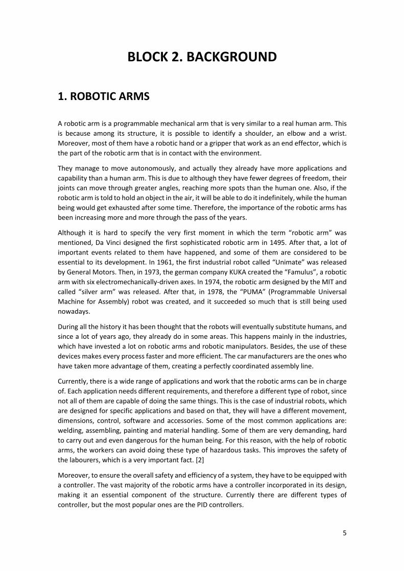
The signal responses have certain properties that define the behaviour of themselves. These properties are:

Rise time: it is the necessary time for a signal to change from a very low value to a very high value. Generally, it measures the time that it takes the signal to go from its 10% to its 90%. Clearly, it is preferred to have a short rise time so as to have a faster response.

Overshoot: it measures how much the signal exceeds its target value. It represents the difference between the maximum signal value and the stabilised value.

Peak time: it is the time it takes the signal to reach its first peak.

Settling time: it is the time that it takes the signal to become steady. This occurs when the signal is in the range of its 2% and 5% final value.

Steady-state error: it represents the difference between the final value of the signal and the value it has when it already becomes steady.

All these properties are clearly pointed out in the following random signal [3]:

7

Figure 1. Properties of a signal.

2.2. PROPORTIONAL ACTION

The proportional action equation is the following one:

𝑢 (𝑡) = 𝐾 𝑒(𝑡) (1)

The proportional gain is 𝐾 , and it is called proportional because it is proportional to the error signal e(t). This action reduces the error by increasing the gain 𝐾 , although It does not ensure a null-steady state error. Obviously, as desired, this action affects the closed-loop behaviour, but not always in a good way. It can produce non-desired oscillations and instability in the outputs if the gain is too high. Besides, when the gain is increased, the rise time decreases and the overshoot increases. [4]

2.3. INTEGRAL ACTION

The integral action equation is the following one:

8

𝑢(𝑡) = 𝐾 𝑒(𝑡 ) 𝑑𝑡 (2)

The integral gain is 𝐾 , and this action changes the inputs of the process based on the accumulated error, therefore it is said that this action “looks” at the past. The integral action usually eliminates or reduces a lot the steady-state error, so improves the steady-state behaviour if the system is stable. However, if the gain is too small it will not make any effect, and if it is too big, it may cause oscillations. As well as the proportional gain, when the integral gain increases, the rise time decreases and the overshoot increases.

2.4. DERIVATIVE ACTION

The derivative action equation is the following:

𝑢(𝑡) = 𝐾 𝑑𝑒(𝑡)

𝑑𝑡 (3)

The derivative action is 𝐾 , and this action is sometimes called “anticipatory” control because it “looks” at the future error. When the gain is increased, it decreases the overshoot and the settling time, and sometimes it also improves the stability if its value is small. On the other hand, it hardly has effect on the rise time and the steady-state error.

As it can be seen, the three control actions has its advantages and its disadvantages, so an equilibrium must be found. What is already clear is that the combination of them three, the PID control action, is the best choice when it is desired to implement a controller in a system. However, it is not easy to find the values of the three gains. There are some methods that help the designer to reach these values, which are called “tuning methods”.

9

3. TUNING METHODS TO OBTAIN THE PID PARAMETERS

Tuning is the tool by which the parameters of the PID controllers are obtained. Each system represents a complete new world and it can have very different requirements. Therefore, each system will need a different control response so as to reach a certain behaviour. Generally, every system shares the will of having a great stability, a null overshoot, a null steady-state error and a minimum rise time. However, this is not always possible, so the designers have to sacrifice some of these benefits and look for a trade-off. In the process of designing the control action, the proportional, integral and derivative gains are obtained. These three gains can be acquired in some different ways, and the most popular ones are going to be described hereunder.

3.1. MANUAL TUNING

This method is carried out by looking at the system response, analysing it and applying the necessary gains. Depending on the response, the designer has to know which action the system needs to improve its behaviour. Therefore, this task must be done by an expert who knows how, when and in which quantity apply the three different gains (P, I and D). After applying the control action, the designer has to look again at the response and come up with the new changes in the control action to improve again the response. This process has to be repeated several times until meeting the requirements or until reaching the best system response possible.

Normally, the next procedure is followed: the three gains 𝐾 , 𝐾 and 𝐾 are set to zero. Then, 𝐾 is slowly increased until observing some oscillations in the output. At this moment, 𝐾 is set to its half so as to have a "quarter amplitude decay" type response. This means that the period is reduced to its fourth part and the transient response becomes faster. However, a little overshoot may occur, so the 𝐾 should be even smaller than its half. Then, 𝐾 has to be increased little by little until correcting the offset and eliminate the steady-state error. It has to be taken into account that a high integral gain could cause instability. After doing this, the controller is sometimes well defined, but if it is desired to have a faster response, 𝐾 is increased. However, it will introduce overshoot if this gain is too big.

If these steps are followed carefully, it is likely that the three obtained gains improve the system response. Nevertheless, the gains might not be really accurate since this is a rudimentary way of obtaining the PID parameters.

As this is a “trial and error” method, it is very important to know what does exactly each gain. Therefore, in the following table are described the effects of each gain into the system behaviour when the gains increase.

10

Parameter Rise Time Overshoot Settling Time Steady-state error

Stability

𝐾 Decrease Increase Small change Decrease Degrade 𝐾 Decrease Increase Increase Eliminate Degrade 𝐾 Minor

Change Decrease Decrease No effect Improve if

𝐾 is small

Table 1. Effects of the signal characteristics when the gain parameters increase.

3.2. ZIEGLER-NICHOLS METHOD

This method was introduced in the 1940s by John G. Ziegler and Nathaniel B. Nichols. It starts with 𝐾 and 𝐾 being set to 0. Then, 𝐾 is increased until the system starts oscillating constantly. The value of this proportional gain is called 𝐾 , and the period of this oscillations is called 𝑇 . These two values have to be obtained with the maximum precision because they will be essential in the process. This is because from the two values, the following table that defines the values of the three gains can be calculated.

Control Type 𝐾 𝐾 𝐾 P 0.5 𝐾 - - PI 0.45 𝐾 0.54 𝐾 / 𝑇 -

PID 0.6 𝐾 1.2 𝐾 / 𝑇 3 𝐾 𝑇 /40

Table 2. Ziegler-Nichols table for obtaining the parameters of the control action.

3.3. SOFTWARE TOOLS TUNING

Currently there are several software’s that ease a lot the process of getting the PID controller. They collect all the data and then they create a model and suggest a certain tuning based on the data. They have a mathematical model that induces an impulse to the system and based on the response, they apply the necessary gains. Most of the companies prefer to use this method instead of the previous ones because it is faster and much more efficient. The other methods are usually very time-consuming and their results are not optimal, so generally, software methods are chosen.

Three of these software’s are Matlab, BESTune and Expertune, although Matlab and Simulink are the ones that are going to be used in this paper. For designing the control action, the software ask the user to specify the requirements or the desired behaviour of the output signal. And then, based on that, the programme tries to reach that signal. Normally, they obtain the parameters with great accuracy, so that is why they are widely known and popular.

11

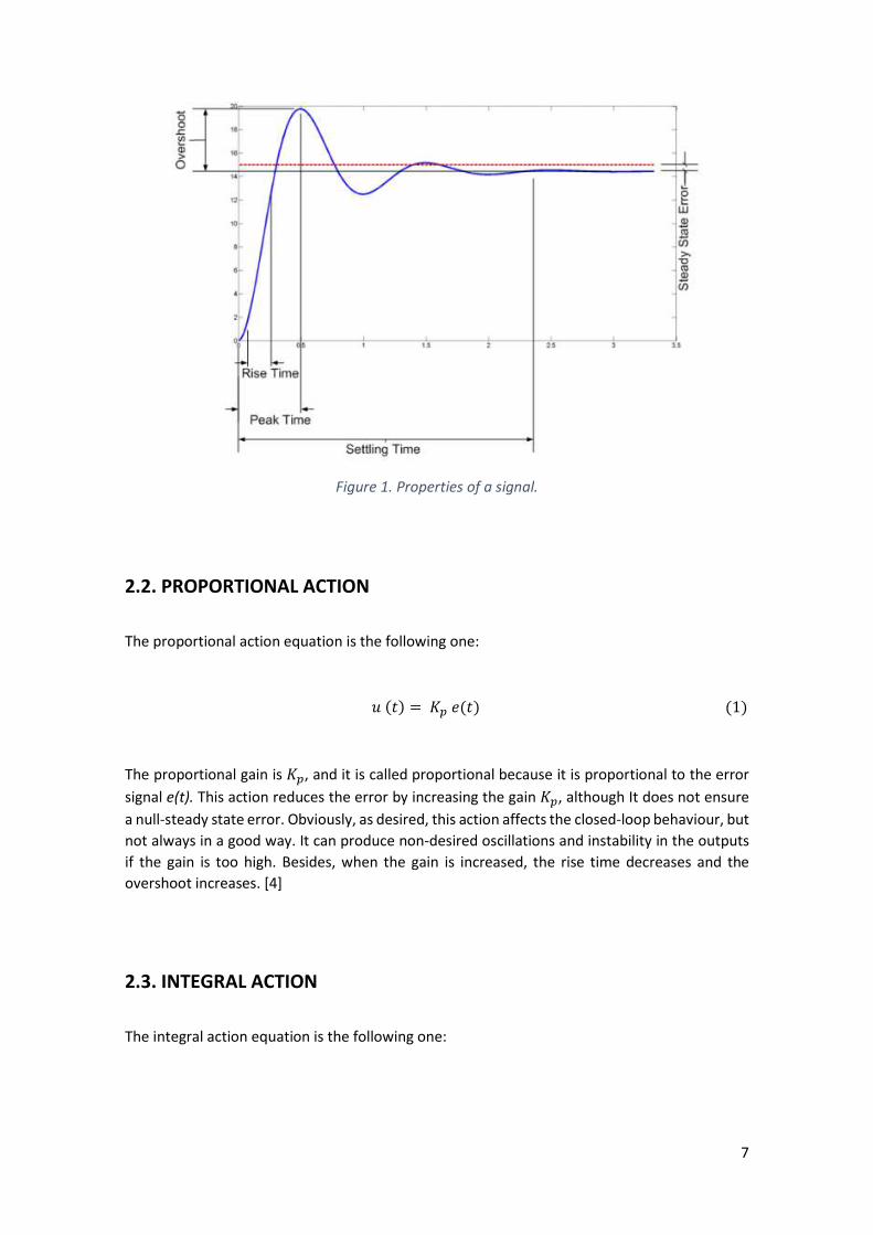
In Simulink, it is used the “PID Controller” block. This blocks represents a PID controller, so the designer can directly insert the values of the gains inside the block. Also, there is the option of “Tune”, in which Matlab linearizes the system and applies an input step and shows how would be the output for that linear system. [5]

The Figure 2 depicts the window that appears when the “Tune” option is pressed. The signal represented is a random signal that Matlab has tuned. In this case it is not a good tuning because it has oscillations, so the signal can be tuned manually with the two sliders at the top. The first slider controls the response time, making it slower or faster. And the second slider controls the transient behaviour, which is between the aggressive and robust behaviour. When moving the sliders, the signal changes automatically, and the values of the three gains can be seen in real time if the option “Show Parameters” at the right is pressed. Besides, it shows the overshoot, rise time, settling time, peak value and stability.

Figure 2. PID tuner window

Once the obtained signal is considered to be correct, the option “Update Block” at the top-right has to be pressed to update the gains of the PID controller block, and therefore, the controller is finally well-designed.

12

BLOCK 3. ANALYSIS AND IMPLEMENTATION OF THE ROBOTIC ARM

1. INTRODUCTION

The main objective of this paper is to pose the mathematical model of a robotic arm and to design its control. The task of this robotic arm is to move towards an object and grab it adequately so as to lift it. To accomplish this job, an image processing stage has to be developed in order to identify the shape of any random object. And only once the object has been identified, the robotic arm will know how much force needs to apply to the object so as to grab it without breaking or dropping it.

Therefore, the whole process that the robotic arm undergoes is divided into two stages: the one already mentioned, the image processing stage, and the second one, which is the dynamics and control stage.

The image processing stage begins with a camera attached to the base of the robotic arm that keeps taking pictures of the environment. These pictures are processed by means of applying different filters. By doing so, the system is able to detect if there is any object in front of the robotic arm or not. Besides, it can also identify some essential features of the objects that characterize themselves. This intrinsic information of the objects is translated into the amount of force that the arm has to execute so as to successfully grab it. This study is made because it is not possible to apply the same force to everything since the shape and fragility differs among the objects. That means that when the object is very fragile or very narrow, less force should be applied for not breaking it. And in the case when the object is very wide or heavy, more force should be applied so that it does not slip. Moreover, a database is also created that stores all the identified objects with their respective pictures and characteristics.

In the dynamics and control stage, the overall structure of the robotic arm is presented. It is made of a combination of links and joints that move freely within its several constraints. It is desired to make the arm move from one position to another, so a mathematical model of the arm is made to control its position at every instant. This model is focused on the joints, which will give the user an accurate location of the arm depending on the angle of the links with respect to its local reference. For reaching this target, the model is based on a set of non-linear, second order and ordinary differential equations. After that, the Lagrange-Euler methodology is employed to simulate the dynamics of the robot. The Newton-Euler methodology could have also been chosen for fulfilling the dynamics, but the Lagrange-Euler one, which is based on the energy of the joints, is considered to be simpler. Moreover, the different links of the arm have to be decoupled so as to move with a higher freedom. And finally, two PID controllers are designed in order to assure a great performance of the robotic arm movements. They both share the same purpose of ensuring a minimal overshoot, a null position error and a minimum rise time. This is all designed in a closed loop so that there is a constant feedback and update of the position of the joints. [6]

13

2. ANALYSIS OF THE DYNAMICS AND CONTROL STAGE

2.1. STRUCTURE OF THE ROBOTIC ARM

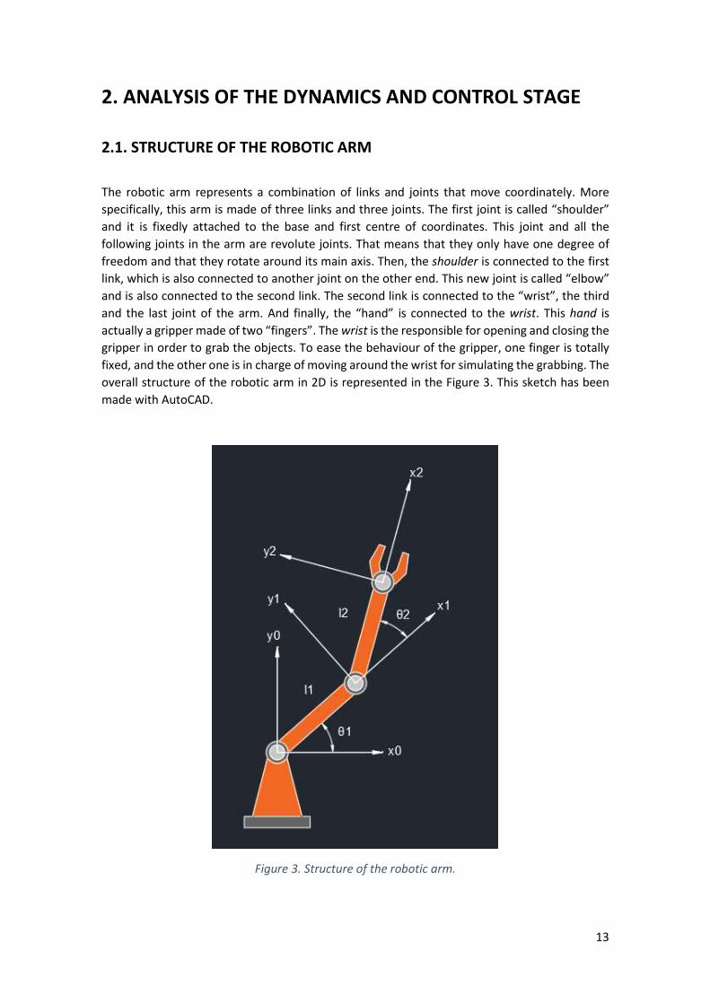
The robotic arm represents a combination of links and joints that move coordinately. More specifically, this arm is made of three links and three joints. The first joint is called “shoulder” and it is fixedly attached to the base and first centre of coordinates. This joint and all the following joints in the arm are revolute joints. That means that they only have one degree of freedom and that they rotate around its main axis. Then, the shoulder is connected to the first link, which is also connected to another joint on the other end. This new joint is called “elbow” and is also connected to the second link. The second link is connected to the “wrist”, the third and the last joint of the arm. And finally, the “hand” is connected to the wrist. This hand is actually a gripper made of two “fingers”. The wrist is the responsible for opening and closing the gripper in order to grab the objects. To ease the behaviour of the gripper, one finger is totally fixed, and the other one is in charge of moving around the wrist for simulating the grabbing. The overall structure of the robotic arm in 2D is represented in the Figure 3. This sketch has been made with AutoCAD.

Figure 3. Structure of the robotic arm.

14

As it can be seen, there are three reference frames. The reference frame ‘0’ is attached to the shoulder, the frame ‘1’ is attached to the elbow and the frame ‘2’ is attached to the wrist. The parametric coordinates of the reference frames are labelled as 𝑥 and 𝑦 , where x represents the horizontal coordinate and y represents the vertical coordinate respect to the ith joint.

On the other hand, link 1 (l1) represents the link that joins the shoulder and the elbow and the link 2 (l2) joins the elbow and the wrist. The angle 𝜃 is defined as the angle between the link 1 and the axe 𝑥 . And the angle 𝜃 is defined as the angle formed by the link 2 and the axe 𝑥 .

What actually makes the link 1 rotate is the rotation exerted by the shoulder joint, and what makes the link 2 move is the rotation of the elbow joint. Although it is important to know the location of the wrist, its rotation doesn’t take part in the analysis because it does not affect the position of the arm. Its only functionality is to enable the opening and closing of the gripper.

Actually, the orientation of the wrist is 90° reversed in the figure 1 in order to see its shape properly. In real life, the wrist would be rotated to grasp the objects across its width. This change in the drawing has only been made to ease the visualization of the gripper and because it does not affect the study at all.

Before starting to analyse the movement of the arm, it is important to know the number of degrees of freedom of the arm as a whole. But, what are exactly the degrees of freedom? As the references [7] and [8] say, the degrees of freedom (DOF) represent the minimum number of independent variables required to define the location of a body in the space. It also defines the number of directions that the body can move through. If the DOF is equal to 0, the body is a fixed structure, and if it is more than one, it is called a mechanism. For calculating the DOF of any body, the Grubler’s equation needs to be applied:

𝐷𝑂𝐹 = 3 (𝑁 − 1) − 2𝑙 − ℎ (4)

Where N is the number of links + the base, l is the number of lower pairs and h is the number of higher pairs. In this case, thee three joints are revolute joints, which are lower pairs.

As N = 4, l = 3 and h = 0, the degrees of freedom (DOF) of the body are equal to 3. Therefore, it can be said that the robotic arm can move into 3 directions, which matches with the 3 revolution joints movements.

2.2. MATHEMATICAL MODEL OF THE ROBOTIC ARM

First of all, it is necessary to state some assumptions that directly influence on the arm behaviour:

- In the real design there would be a DC motor attached to each revolute joint. Hence, three stepper motors would be fed with constant voltage and would allow the movement of the links. However, the dynamics of these actuators are not taken into account in this paper. This decision eases the mathematical model and calculations.

15

- The masses of the first two links are assumed to be concentrated at the end of each link. And the mass of the gripper is considered to be negligible due to its low impact in the design.

- The friction forces are assumed to be negligible, so the arm is working in an ideal situation.

The second step is to define the position of the two reference frames. [9]

𝑥 = 𝑙 sin(𝜃 ) (5)

𝑦 = 𝑙 cos(𝜃 ) (6)

𝑥 = 𝑙 sin(𝜃 ) + 𝑙 sin(𝜃 + 𝜃 ) (7)

𝑦 = −𝑙 cos(𝜃 ) − 𝑙 cos(𝜃 + 𝜃 ) (8)

It could be thought that the horizontal coordinate is obtained with the cosine and the vertical coordinate with the sine. This assumption is true if the methodology employed would be another one, but in this design the aim is to define the three reference frames. That means that the equation 5 computes the necessary value to go from 𝑥 to 𝑥 and the equation 6 carries the necessary value to go from 𝑦 to 𝑦 . With this, the reference frame of the elbow is defined. This step should be repeated for defining the location of the reference frame of the wrist, which would be done by calculating the equations 7 and 8. [10]

As mentioned before, the Lagrangian approach is based on the energy of the system. Consequently, the next step is to obtain the kinetic and potential energy of the joints. [11]

The kinetic energy is defined as:

𝐾 = 𝑚 𝑣

2 (9)

Therefore, the kinetic energy of the system is:

𝐾 = 𝑚 𝑣

2+

𝑚 𝑣

2 (10)

Where 𝑚 is the mass of the first link, 𝑚 is the mass of the second link, 𝑣 is the velocity of the first joint and 𝑣 is the velocity of the second joint.

The velocities are unknown, but they can be calculated by means of the derivative of the position respect to the time.

The first derivative of an angle has a dot above the ‘𝜃’, and the second derivative has two dots.

16

𝑣 = 𝑑

𝑑𝑡

𝑥𝑦 =

𝑙 cos(𝜃 ) 𝜃 ̇

−𝑙 sin(𝜃 ) 𝜃̇ (11)

𝑣 = 𝑑

𝑑𝑡

𝑥𝑦 =

𝑙 cos(𝜃 ) 𝜃̇ + 𝑙 cos(𝜃 + 𝜃 ) 𝜃 ̇ 𝜃 ̇

𝑙 sin(𝜃 ) 𝜃̇ + 𝑙 sin(𝜃 + 𝜃 ) 𝜃̇ 𝜃 ̇ (12)

Moreover, to reduce the complexity of the calculus, the following abbreviations will be used from now on:

𝑠 = sin(𝜃 ) , 𝑐 = cos(𝜃 ) , 𝑠 = sin(𝜃 + 𝜃 ) 𝑎𝑛𝑑 𝑐 = cos(𝜃 + 𝜃 )

In order to obtain the velocity square, the transpose of the velocity vector has to me multiplied to the velocity vector.

𝑣 = ‖𝑣‖ = 𝑣 𝑣 (13)

𝑣 = [ 𝑙 𝑐 𝜃̇ −𝑙 𝑠 𝜃̇ ] 𝑙 𝑐 𝜃̇

−𝑙 𝑠 𝜃̇ (14)

𝑣 = 𝑙 (𝑐 + 𝑠 ) 𝜃̇ = 𝑙 𝜃̇ (15)

After obtaining 𝑣 , 𝑣 is obtained in the same way:

𝑣 = [ 𝑙 𝑐 𝜃̇ + 𝑙 𝑐 𝜃̇ 𝜃 ̇ 𝑙 𝑠 𝜃̇ + 𝑙 𝑠 𝜃̇ 𝜃 ̇ ] 𝑙 𝑐 𝜃̇ + 𝑙 𝑐 𝜃̇ 𝜃 ̇

𝑙 𝑠 𝜃̇ + 𝑙 𝑠 𝜃̇ 𝜃 ̇ (16)

𝑣 = 𝑙 𝑐 𝜃 + 2𝑙 𝑙 𝑐 𝑐 𝜃̇ + 𝜃̇ 𝜃 + 𝑙 𝑐 (𝜃̇ + 𝜃 ̇ ) + 𝑙 𝑠 𝜃̇

+ 2𝑙 𝑙 𝑠 𝑠 𝜃̇ + 𝜃̇ 𝜃 + 𝑙 𝑠 (𝜃̇ + 𝜃 ̇ ) (17)

𝑣 = 𝑙 𝜃̇ + 𝑙 𝜃̇ + 𝜃 ̇ + 2 𝜃̇ 𝜃 ̇ + 2 𝑙 𝑙 𝑐 𝜃 ̇ + 𝜃̇ 𝜃 ̇ (18)

And finally, if the equations (15) and (18) are substituted in the equation (10), the final kinetic energy of the body is the following:

17

𝐾 = 1

2 𝑚 𝑙 𝜃̇ +

1

2 𝑚 𝑙 𝜃̇ +

1

2 𝑚 𝑙 𝜃̇ + 𝜃 ̇ + 2 𝜃̇ 𝜃 ̇

+ 𝑚 𝑙 𝑙 𝑐 𝜃̇ + 𝜃̇ 𝜃 ̇ (19)

𝐾 = 1

2 (𝑚 + 𝑚 ) 𝑙 𝜃̇ +

1

2 𝑚 𝑙 𝜃̇ + 𝜃 ̇ + 2 𝜃̇ 𝜃 ̇

+ 𝑚 𝑙 𝑙 𝑐 𝜃̇ + 𝜃̇ 𝜃 ̇ (20)

The next step is to calculate the potential energy, represented in the equation (21).

𝑃 = 𝑚 𝑔 ℎ (21)

Where m is the mass of the joint, g is the gravity acceleration and h is the height of the joint respect to the first reference frame.

If the equation (21) is applied to the two joints, the following equation is obtained:

𝑃 = −(𝑚 + 𝑚 ) 𝑔𝑙 𝑐 − 𝑚 𝑔𝑙 𝑐 (22)

After that, it is already possible to calculate the Lagrangian equation L, which is defined as the difference between the kinetic and potential energy.

𝐿 = 𝐾 − 𝑃 (23)

Once the Lagrangian is calculated, it is already possible to solve the Euler-Lagrange equation defined in the equation (24).

𝜏 = 𝑑

𝑑𝑡

∂L

∂�̇�−

∂L

∂𝜃 (24)

This equation is considered to be the equation of motion of the dynamic system. By means of a set of partial derivatives of the Lagrangian respect to the angle and its derivative, the torque 𝜏 is obtained. This torque represents the external force applied to a joint so that it moves to a certain position. It is the force in charge of executing the rotatory movement of the revolution joints. There are two different torques in this robotic arm: one applied to the shoulder and one applied to the elbow.

The torque of the shoulder is calculated, but it needs to be done step by step.

18

∂L

∂�̇�= (𝑚 + 𝑚 )𝑙 𝜃̇ + 𝑚 𝑙 𝜃̇ + 𝜃 ̇ + 2 𝑚 𝑙 𝑙 𝑐 𝜃̇

+ 𝑚 𝑙 𝑙 𝑐 𝜃 ̇ (25)

𝑑

𝑑𝑡

∂L

∂�̇�= (𝑚 + 𝑚 )𝑙 + 𝑚 𝑙 + 2 𝑚 𝑙 𝑙 𝑐 �̈� + 𝑚 𝑙 + 𝑚 𝑙 𝑙 𝑐 �̈�

− 2 𝑚 𝑙 𝑙 𝑠 𝜃̇ 𝜃 ̇ − 𝑚 𝑙 𝑙 𝑠 �̈� (26)

∂L

∂𝜃= −(𝑚 + 𝑚 )𝑔𝑙 𝑠 − 𝑚 𝑔𝑙 𝑐 (27)

Then, the equations (25), (26) and (27) are applied to the general equation (24) of the torque, obtaining:

𝜏 = (𝑚 + 𝑚 )𝑙 + 𝑚 𝑙 + 2 𝑚 𝑙 𝑙 𝑐 �̈� + 𝑚 𝑙 + 𝑚 𝑙 𝑙 𝑐 �̈� − 2 𝑚 𝑙 𝑙 𝑠 𝜃̇ 𝜃 ̇

− 𝑚 𝑙 𝑙 𝑠 �̈� + (𝑚 + 𝑚 )𝑔𝑙 𝑠 + 𝑚 𝑔𝑙 𝑠 (28)

The first torque is already calculated, so now the second torque is obtained through the same procedure.

∂L

∂�̇�= 𝑚 𝑙 𝜃̇ + 𝜃̇ + 𝑚 𝑙 𝑙 𝑐 𝜃̇ (29)

𝑑

𝑑𝑡

∂L

∂�̇�= 𝑚 𝑙 �̈� + �̈� + 𝑚 𝑙 𝑙 𝑐 �̈� − 𝑚 𝑙 𝑙 𝑠 𝜃̇ 𝜃 ̇ (30)

∂L

∂𝜃= −𝑚 𝑙 𝑙 𝑠 �̇� + 𝜃̇ 𝜃 ̇ − 𝑚 𝑔𝑙 𝑠 (31)

𝜏 = 𝑚 𝑙 + 𝑚 𝑙 𝑙 𝑐 �̈� + 𝑚 𝑙 �̈� + 𝑚 𝑙 𝑙 𝑠 �̇� + 𝑚 𝑔𝑙 𝑠 (32)

Once both torques are obtained, it is recommended to re-arrange them into the following single form of a non-linear equation:

𝜏 = 𝑀(𝜃)�̈� + 𝐶 𝜃, �̇� �̇� + 𝐺(𝜃) (33)

19

Where 𝜃 Є 𝑅 represents the link positions and n represents the joint numbers, which in this case is 2. 𝑀(𝜃) is the inertia matrix, 𝐶 𝜃, �̇� represents the centrifugate force and 𝐺(𝜃) represents the gravity force. They are defined as:

𝑀(𝜃) = (𝑚 + 𝑚 )𝑙 + 𝑚 𝑙 + 2 𝑚 𝑙 𝑙 𝑐 𝑚 𝑙 + 𝑚 𝑙 𝑙 𝑐

𝑚 𝑙 + 𝑚 𝑙 𝑙 𝑐 𝑚 𝑙 (34)

𝐶 𝜃, �̇� = −2 𝑚 𝑙 𝑙 𝑠 𝜃̇ 𝜃 ̇ − 𝑚 𝑙 𝑙 𝑠 �̇�

𝑚 𝑙 𝑙 𝑠 �̇� (35)

𝐺(𝜃) = (𝑚 + 𝑚 )𝑔𝑙 𝑠 + 𝑚 𝑔𝑙 𝑠

𝑚 𝑔𝑙 𝑠 (36)

2.3 CONTROL STRATEGY

The purpose of the robotic arm is to reach the two angles given by the user. These desired angles can also be labelled as 𝜃 . However, it is impossible to reach this angle in the very first moment, so the aim of the actual angle 𝜃 is to become the desired angle. Meanwhile, the difference between both angles is called the angle error. It is labelled as 𝜃 and obtained in the equation (37).

𝜃 = 𝜃 − 𝜃 (37)

The ideal behaviour of the robot would occur when the angle error is lower and lower until it becomes null. This task is achieved by the PID controller, which is implemented for ensuring a good performance of the robot work. That means getting the desired angle as fast as possible with a null error and a great stability.

The mathematical model of the arm is working on two different angles, hence there will be needed two different PID controllers, one per link.

As mentioned before, the function of the PID controller is to diminish the error angle. For doing so, the PID control law expression is applied:

𝜏 = 𝐾 𝜃 + 𝐾 𝜃(𝑡) 𝑑𝑡 + 𝐾 �̇� (38)

20

It can be assumed that:

�̇� = 𝐾 𝜃 (39)

Therefore, the equation (38) can be re-written as:

𝜏 = 𝐾 𝜃 + 𝜉 + 𝐾 �̇� (40)

The closed loop equation can be obtained when the equation (33) and (40) are mixed.

Actually, it is important to notice that these both equations are ruled by a torque or a control action. If the control action 𝜏 of the equation (40) is substituted in the robot model of the equation (33), the following closed loop equation of the robotic arm is reached:

𝑀(𝜃)�̈� + 𝐶 𝜃, �̇� �̇� + 𝐺(𝜃) = 𝐾 𝜃 + 𝜉 + 𝐾 �̇� (41)

2.4. THE DECUOPLING EFFECT

The two important links of the robot are dependent on each other due to there is a strong interaction between them. In mechanics, these two links are said to be coupled because one action of one link affects the other one and vice versa. This connection is needed but at some point it will end up making impossible situations like collisions between links. Therefore, the solution is as simply as decoupling them. By doing this, the system allows the arm to move more freely.

According to the book “A mathematical introduction to robotic manipulation” written by Richard M. Murray and published in 1994 [12], it is possible to represent the motion of the end-effector. The work ‘W’ done by the force applied to the links in the time interval 𝑡 to 𝑡 can be calculated as:

𝑊 = 𝜓 𝐹 𝑑𝑡 (42)

Where 𝜓 is the linear velocity vector and F is the force vector that is applied to the end effector.

In the intention of relating this equation to the robotic arm model, it can be deduced that 𝜓 is the same as �̇�, the first derivative of the angle of the arm. Moreover, the external force F is the

21

same as the torque 𝜏 applied to the joints. Therefore, it is assumed that the work of the equation (42) is the same work performed by the robotic arm.

𝑊 = 𝜓 𝐹 𝑑𝑡 = �̇� 𝜏 𝑑𝑡 (43)

On the other side, if the following equality is assumed:

𝜓 = 𝐽 �̇� (44)

The equation (43) can be further developed into:

𝑊 = 𝐽 �̇� 𝐹 𝑑𝑡 = �̇� 𝜏 𝑑𝑡 (45)

𝐽 �̇� 𝐹 = �̇� 𝜏 (46)

𝜏 = 𝐽 𝐹 (47)

It can be noticed that the equation (47) relates the torque and the force by means of the transpose of J. This force F is the output of the PID controller and the torque 𝜏 is the input of the robotic arm necessary to make it move from one angle to another. The variable J is the Jacobian matrix, which is in charge for decoupling the two links.

This approach can be graphically seen in the Figure 4.

Figure 4. Closed loop system for the robotic arm.

22

The Figure 4 is an overall representation of the modus operandi of the robotic arm. It starts with the desired angle 𝜃 as the reference of the system. Then the error is calculated as the difference between the reference and the output angle. This error is processed by the PID controller and it calculates the necessary force F to rectify this error. The obtained force F needs first to be decoupled before being applied to the arm. Therefore, it has to go through the decoupling block. The output of the block is the torque 𝜏, which is the input of the robotic arm. This torque is applied to the joints, and as a result, the arm moves towards another angle. This angle is called the actual angle and it will be subtracted to the reference angle in order to repeat the whole process again.

The last step to finish the decoupling block is to define the Jacobian vector:

The variable x is defined as the Cartesian coordinates of the joint position vector 𝜃 = [𝜃 𝜃 ] . Also assume that:

𝑥 = ℎ(𝜃) = ℎ (𝜃)ℎ (𝜃)

(48)

Where ℎ(𝜃) is a function between the Cartesian coordinates and the angle position. This function exactly represents the position of the second reference frame, which is defined in the equations (7) and (8). Therefore:

𝑥 = ℎ(𝜃) = ℎ (𝜃)ℎ (𝜃)

= 𝑙 sin(𝜃 ) + 𝑙 sin(𝜃 + 𝜃 )

−𝑙 cos(𝜃 ) − 𝑙 cos(𝜃 + 𝜃 ) (49)

After that, the first derivative of the x respect to the angle is computed in the equation (49). This derivative will be �̇�, the linear velocity.

�̇� =𝑑

𝑑𝜃[ℎ(𝜃)] =

𝜕ℎ(𝜃)

𝜕𝜃 �̇� (50)

Besides, it is noted that this linear velocity that has just been obtained, is equal to the variable 𝜓.

�̇� = 𝜓 (51)

Therefore, equations (44) and (50) are joint, forming:

𝜕ℎ(𝜃)

𝜕𝜃 �̇� = 𝐽 �̇� (52)

23

If the �̇� term is crossed at both sides of the equality, the equation concludes in:

𝐽 = 𝜕ℎ(𝜃)

𝜕𝜃 (53)

And if it is further developed, the Jacobian matrix can be defined as:

𝐽 = 𝜕ℎ(𝜃)

𝜕𝜃=

⎣⎢⎢⎡𝜕ℎ

𝜕𝜃

𝜕ℎ

𝜕𝜃𝜕ℎ

𝜕𝜃

𝜕ℎ

𝜕𝜃 ⎦⎥⎥⎤

(54)

𝐽 = 𝑙 cos(𝜃 ) + 𝑙 cos(𝜃 + 𝜃 ) 𝑙 cos(𝜃 + 𝜃 )

𝑙 sin(𝜃 ) + 𝑙 sin(𝜃 + 𝜃 ) 𝑙 sin(𝜃 + 𝜃 ) (55)

So finally, the general relation between the force F and the torque 𝜏 is the following:

𝜏𝜏 =

𝐽 𝐽𝐽 𝐽

𝐹

𝐹 (56)

And the general relation in the equation (56) applied to this robotic arm is:

𝜏𝜏 =

𝑙 cos(𝜃 ) + 𝑙 cos(𝜃 + 𝜃 ) 𝑙 cos(𝜃 + 𝜃 )

𝑙 sin(𝜃 ) + 𝑙 sin(𝜃 + 𝜃 ) 𝑙 sin(𝜃 + 𝜃 )

𝐹

𝐹 (57)

24

3. ANALYSIS OF THE IMAGE PROCESSING STAGE

The image processing stage is highly related to the gripper. This stage has to identify the objects with the help of a camera and send this information to the gripper. However, this information has to be previously processed before sending the gripper a specific command. This process consists on calculating the width of the objects and based on that information, estimate how much the “fingers” would need to be rotated in order to grab the object.

The performance starts with the camera taking random pictures. Then, the system applies a filter to all these images so as to convert them into grayscale. That means having them in the black and white format. After that, the system needs to know if there is actually an object in the image or otherwise, the picture is empty. For checking it, the strategy of the boundaries is applied. This method is based on detecting all the edges of an image, so that if there is any object in front of the arm, the boundaries that build its shape will be detected. There is a wide range of filters that can carry out this task, but one of the best ones is the “Canny filter”. [13]

The canny filter uses an edge detection operator that is applied only to grayscale images, so that is why the previous conversion to grayscale was made. The canny filer is a multi-step algorithm that works in the following way: first, the Gaussian filter is applied to smooth the image, reduce the noise and the unwanted textures. Secondly, the intensity gradients are computed using any of the gradient operators such as Sobel or Prewitt. Then, the non-maximum suppression is applied to eliminate the misleading response of the edge detection. After that, a double threshold is applied to determine the potential edged, and finally, the edges that are weak or not connected to strong edges are suppressed. [14]

The result of this process will be the detection of the edges of the objects. Hence, if there is not any edge detected is because there is not actually any object in front of the arm and therefore it does not need to move. On the contrary, in the case when there is an object, the edges are detected and the robotic arm is enabled to move towards the object. Furthermore, the width of the object in the picture can be measured. Obviously, the size of the objects in the image is not the same than in real life, so this measure in the image must be converted into the size in the reality.

For obtaining this conversion factor, a random object is measured in real life and in the picture. The division between these two measures represents the standard ratio between the width of an object in real life and in the image.

𝑅𝑎𝑡𝑖𝑜 = 𝑤𝑖𝑑𝑡ℎ 𝑜𝑓 𝑎 𝑟𝑎𝑛𝑑𝑜𝑚 𝑜𝑏𝑗𝑒𝑐𝑡 𝑖𝑛 𝑟𝑒𝑎𝑙 𝑙𝑖𝑓𝑒 (𝑐𝑚)

𝑤𝑖𝑑𝑡ℎ 𝑜𝑓 𝑎 𝑟𝑎𝑛𝑑𝑜𝑚 𝑜𝑏𝑗𝑒𝑐𝑡 𝑖𝑛 𝑡ℎ𝑒 𝑝𝑖𝑐𝑡𝑢𝑟𝑒 (𝑐𝑚) (58)

This ratio is obtained with a random object, but this ratio is also valid for any object. Therefore, the general relation between the two measures is expressed in the equation (59)

𝑆𝑖𝑧𝑒 𝑜𝑓 𝑎𝑛𝑦 𝑜𝑏𝑗𝑒𝑐𝑡 𝑖𝑛 𝑟𝑒𝑎𝑙 𝑙𝑖𝑓𝑒 = 𝑅𝑎𝑡𝑖𝑜 ∗ 𝑆𝑖𝑧𝑒 𝑜𝑓 𝑎𝑛𝑦 𝑜𝑏𝑗𝑒𝑐𝑡 𝑖𝑛 𝑡ℎ𝑒 𝑝𝑖𝑐𝑡𝑢𝑟𝑒 (59)

25

This general equation can be applied to any object as long as the distance from the camera and the objects is always the same and also that the dimensions of the picture in pixels remains the same for all the images. The first requirement is fulfilled since the camera is attached to the immobile base of the arm and the objects will be always located in the same position. The second requirement is also fulfilled because the system will ensure that the dimensions of the image do not vary, in this case, they are set to be 1500x2000 pixels.

Once the real size of the width of any object can be calculated, the next step is to know the aperture of the gripper. As mentioned previously, one finger of the gripper will be fixed and the other one will move accordingly to the rotation of the wrist.

When the gripper is closed, the angle between the two fingers is 0°, and when it is completely opened, the angle is 90°. Besides, when the fingers are closed, the distance between the ends of the two fingers is null. And when the gripper is fully opened, the distance between the fingers is the maximum distance allowed before they break down. These two positions are the limits within the gripper can rotate. They are represented in the Figure 5.

Figure 5. Maximum and minimum apertures of the gripper.

Knowing the maximum and minimum distances and rotations, it is possible to obtain a relation between the width of the objects and the rotation that the gripper has to execute to grasp them. The maximum distance between the fingers is set to be 15 cm, so the relation is obtained by dividing the 90° over the 15 cm.

𝑅𝑎𝑡𝑖𝑜 = 𝑚𝑎𝑥𝑖𝑚𝑢𝑚 𝑎𝑛𝑔𝑙𝑒 (°)

𝑚𝑎𝑥𝑖𝑚𝑢𝑚 𝑑𝑖𝑠𝑡𝑎𝑛𝑐𝑒 (𝑐𝑚)=

90°

15 𝑐𝑚= 6 °

𝑐𝑚 (60)

This new ratio represents the relation that the gripper has between its angle and distance, so it enables to build a general equation:

26

𝐴𝑛𝑔𝑙𝑒 𝑜𝑓 𝑡ℎ𝑒 𝑔𝑟𝑖𝑝𝑝𝑒𝑟 = 𝑅𝑎𝑡𝑖𝑜 ∗ 𝑊𝑖𝑑𝑡ℎ 𝑜𝑓 𝑎𝑛𝑦 𝑜𝑏𝑗𝑒𝑐𝑡 (61)

And finally, the angle of the gripper is sent to the revolute joint of the wrist. This joint rotates until reaching this angle and at last, the gripper is grabbing the object.

After performing all these calculations, all the obtained data is stored in a database. Basically, the database saves the width of the objects in the images, the width in real life and the angle that the gripper would need to have. This information is saved for further analysis.

27

4. IMPLEMENTATION OF THE DYNAMICS AND CONTROL STAGE IN MATLAB

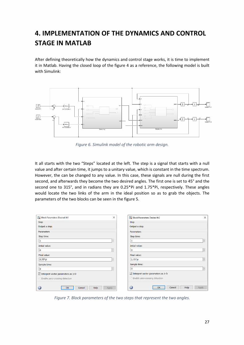
After defining theoretically how the dynamics and control stage works, it is time to implement it in Matlab. Having the closed loop of the figure 4 as a reference, the following model is built with Simulink:

Figure 6. Simulink model of the robotic arm design.

It all starts with the two “Steps” located at the left. The step is a signal that starts with a null value and after certain time, it jumps to a unitary value, which is constant in the time spectrum. However, the can be changed to any value. In this case, these signals are null during the first second, and afterwards they become the two desired angles. The first one is set to 45° and the second one to 315°, and in radians they are 0.25*Pi and 1.75*Pi, respectively. These angles would locate the two links of the arm in the ideal position so as to grab the objects. The parameters of the two blocks can be seen in the figure 5.

Figure 7. Block parameters of the two steps that represent the two angles.

28

After that, there are two “Sum Blocks”. They carry out the difference between the desired angles and the output angles. The result is the error angle signal, which is the input to the PID controllers. The controllers process these two erros and set up the two outputs, the forces F1 and F2.

The two forces and the two angles are the input of the “Decoupling” Matlab function Block. This type of blocks work in the following way: they receive the input signals, apply on them some process implemented on a script and then they obtain some outputs. Once you enter in the block, the following sub-block with the corresponding inputs and outputs is found:

Figure 8. Sub-block of the Decoupling block.

This sub-block is in charge of decoupling the two links. So basically, it takes the forces and multiply them by the Jacobian matrix in order to obtain the two torques: tau 1 and tau 2. The calculus of the Jacobian matrix is done in an external script because otherwise it gives problems. This script is the following:

Figure 9. Matlab script where the Jacobian matrix is calculated.

29

Once the Jacobian matrix is calculated, the decoupling block can start to work. If it is double clicked on the sub-block, the following script is found:

Figure 10. Script in the Matlab function block “Decoupling”.

Then, these output signals are the input of the following Matlab function block, called “Robotic Arm”. This block also needs the two angles and their first derivatives as inputs. Inside the block, it can be seen:

Figure 11. Sub-block of the Robotic arm.

Note that the first derivative of the angles are called w1 and w2, and the second derivative of the angles are called alpha 1 and alpha 2.

30

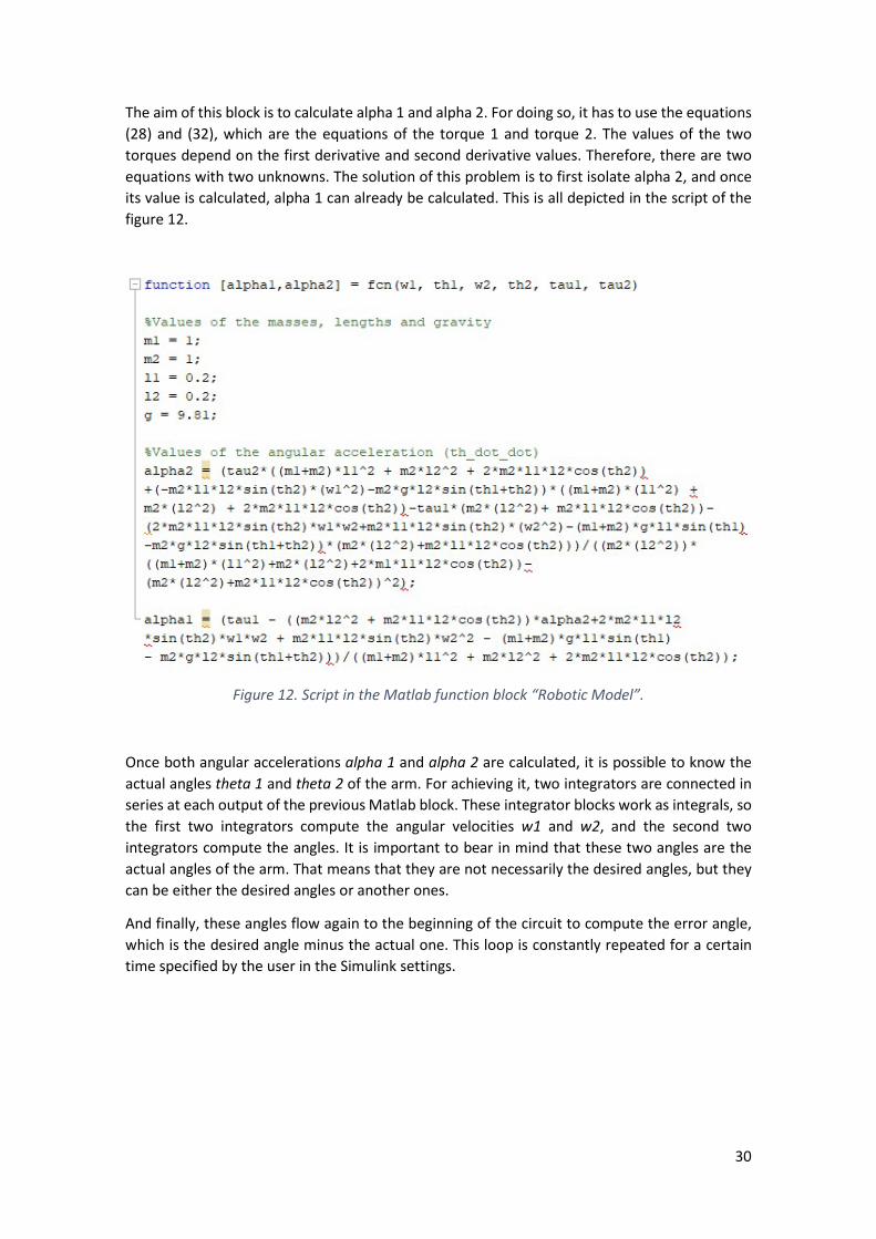
The aim of this block is to calculate alpha 1 and alpha 2. For doing so, it has to use the equations (28) and (32), which are the equations of the torque 1 and torque 2. The values of the two torques depend on the first derivative and second derivative values. Therefore, there are two equations with two unknowns. The solution of this problem is to first isolate alpha 2, and once its value is calculated, alpha 1 can already be calculated. This is all depicted in the script of the figure 12.

Figure 12. Script in the Matlab function block “Robotic Model”.

Once both angular accelerations alpha 1 and alpha 2 are calculated, it is possible to know the actual angles theta 1 and theta 2 of the arm. For achieving it, two integrators are connected in series at each output of the previous Matlab block. These integrator blocks work as integrals, so the first two integrators compute the angular velocities w1 and w2, and the second two integrators compute the angles. It is important to bear in mind that these two angles are the actual angles of the arm. That means that they are not necessarily the desired angles, but they can be either the desired angles or another ones.

And finally, these angles flow again to the beginning of the circuit to compute the error angle, which is the desired angle minus the actual one. This loop is constantly repeated for a certain time specified by the user in the Simulink settings.

31

5. IMPLEMENTATION OF THE IMAGE PROCESSING STAGE IN MATLAB

For checking the reliability of this stage, it is decided to test 5 different objects with different sizes. Therefore, one picture of each object is taken and loaded into a new script in Matlab. [15]

The first step is to read the image and to assign it to a variable, so the command “imread” is employed. Then, the command “im2bw” is used to convert the image to grayscale. And finally, the canny filter is applied to obtain the boundaries of the image. This last command is the following:

Figure 13. Matlab command of the Canny filter.

The obtained a variable saves the image with the detected edges, the obtained variable b collects the two thresholds of the canny filter and variable is the input image. After that, both the image of the object and the image with the boundaries are plot in the same figure. The whole aforementioned process is repeated and applied five times to the five images. It can be seen in the figure 14.

32

Figure 14. First Part of the Image processing stage script.

Then, it is time to calculate the real width of the objects. But first, the standard ratio must be obtained. Therefore, the first object, the “bottle” is measured in real life and in the picture. In real life, its width measures 6.5 cm, and in the picture, it measures 3 cm. So the general ratio is simply the division of 6.5 over 3. After that, the 5 variables of the widths in the pictures are declared. And finally, the real widths are obtained by multiplying the previous 5 variables to the standard ratio. This is all done in the following figure:

Figure 15. Second part of the image processing stage script.

33

The next step is to calculate the ratio that relates the real width of the objects to the angle of the gripper. As stated in the theoretical part, the ratio is the division of 90° over 15 cm. And then, the five angles are just obtained by multiplying this ratio with the real widths.

Figure 16. Third part of the image processing stage script.

This would be the last part of the process, since these angles are sent to the revolute joint of the wrist so as to make it rotate. However, it is a good idea to store all this values in a database. This database is described in the figure 17.

Figure 17. Fourth part of the image processing stage script.

As it can be seen, the first column collects the names of the objects, the second column has the sizes in the images, the third column has the sizes in real life and the fourth column has the angles of the gripper.

34

BLOCK 4. SIMULATION AND ANALYSIS OF THE RESULTS

1. SIMULATION OF THE DYNAMICS AND CONTROL STAGE

1.1. DESIRED BEHAVIOUR OF THE SYSEM

What is actually being controlled is the movement of the arm, more concretely the angles of the links. Therefore, if the system response has overshoot, it would make the arm shaking during its performance, which is unacceptable to have. After that, in the steady state it is important to have a null steady-state error because otherwise it would also make the arm shake when grabbing the objects. Besides, it is essential that the system is stable because an unstable system is unpredictable and can cause many fatal errors. Therefore, these three properties (overshoot, steady-state error and stability) have to be taken into account in the very first moment.

Once they are checked, then it is already the moment to check the properties related to time, such as: rise time, settling time and peak time. They indicate the speed of the system, a very important fact because it is good to have a fast response. Therefore, when these times are reduced without affecting any other property, the response behaviour is improved.

The next step is to classify the system in one of the four types of damping that relates the output with the steady-state response. The figure 18 classifies the four possible responses depending on the type of damping and their damping ratio.

In purpose of the desired response, the underdamped and undamped ones are totally discarded because they have an oscillatory response. Then, the election is between the overdamping and the critically damping system. Both of them ensure no oscillations in the output, but the overdamping system tends to be slower, so the choice is to have a critical damping system.

Figure 18. Type of responses

35

The critical damped response has a short rise time, a great stability, null overshoot and null steady-state error. Hence, this signal gathers the basic requirements and it is the role model.

1.2. ACTUAL BEHAVIOUR OF THE SYSTEM

The system built in Simulink based on the mathematical model represents a big challenge for the PID controller design. This is because there are two controllers working consecutively, where both of them strongly depend on each other. Each of the two outputs of the first Matlab block (the two torques), depend on the two outputs of the controller (the two forces). And then, each of the two angles (theta 1 and theta 2), depend on both torques. This means that each controller output is affecting the behaviour of the other controller, so each change applied to either one of them, will consequently alter the other one. Besides, the two Matlab blocks have feedback from the two angles, so this leads to having everything interconnected and multi-dependent. Moreover, it is important to add that this system is based on a non-linear model, making harder the implementation and the simulation.

This whole dependency makes the designing extremely difficult, only within the reach of the software tuning. Anyways, both the manual tuning and the Ziegler-Nichols methods have been performed, but with poor results.

In the manual tuning, after setting 𝐾 and 𝐾 of both controllers to 0 and making both responses oscillatory, it is impossible to adjust the other parameters. When the integral gain of the first controller is adjusted, theta 2 is messed up. And when this mess is fixed by changing the values of the second controller, theta 1 changes to a random wrong value. This means that the first controller is in charge of both angles and the second controller too. So definitely, it is impossible to have a good response in one angle and not spoil the other one. One example is the following, in which theta 1 is not even close to the ideal behaviour.

Figure 19. Signal of theta 1

36

Obviously, this performance lacks everything, but unfortunately is one of the best responses obtained with manual tuning. The signal of theta 2 is even worse, so it can be said that this tuning method is not effective in this system.

In the Ziegler-Nichols method, both oscillatory responses and the values of 𝐾 and 𝑇 are obtained. But after that, when the table 2 of the gain values is applied, the angles are far from the values they should be. They can be seen in the following figures.

Figure 20. Theta 1 response with Ziegler-Nichols method.

Figure 21. Theta 2 response with Ziegler-Nichols method.

37

As noted, these signals are really wrong and this method is not effective in this system either.

Therefore, software tuning is the only reliable method for this system. When the “Tune” option is pressed, the response is available to be changed by moving the two sliders at the top. In this way, the signal is obtained by tuning it graphically, without taking into account the parameters of the three gains. The first tuned signal with its parameters is represented below:

Figure 22. Tuner response of the first PID controller

Figure 23. Parameters of the first PID controller.

38

And the second tuned signal with its parameters is represented hereunder:

Figure 24. Tuner response of the second PID controller.

Figure 25. Parameters of the second PID controller.

.

39

As noted, the two signals characteristics are brilliant. Their rise time and settling time are almost in terms of micro seconds and the overshoots are 0.356% for the first controller and 0% for the second one. Besides, both responses are stable and they seem to have a null steady-state error.

However, the values of the gains are really big, so it is very hard and time-consuming for a computer to load. So, when the Simulink file is run, the software is not capable of running such huge parameters of the controller. The solution is to have an adequate “Solver” and a tiny fixed step-size as shown in the figure 26. This is adjusted in the “Model Settings” in Simulink.

Figure 26. Model Settings of Simulink.

The step size might be too small, but if it is not tiny, Simulink will not run it. And the smaller it is, the longer it takes it to run.

However, in this case, no matter how much little the step size is set, the software will not run it for a decent span time like 10 seconds. It is not even able to run it for more than a second, and hence, it is impossible to see properly the response behaviour.

Anyway, although the software cannot run the actual outputs, the two PID controllers characteristics are close to the perfection, so it is likely that the actual angles follow successfully the behaviour of the desired angles. Besides, the overshoot, the rise time and the settling time parameters of the controllers are so good, that there is a big space of error allowed. This means that in the case that the responses get worse, they would be still doing an accurate performance. This is because the controller parameters are so accurate and precise that everything should be really messed up to have a bad output response.

40

2. SIMULATION OF THE IMAGE PROCESSING STAGE

When the script is run, all the images are loaded and all their boundaries are generated. Five different figures are obtained, and each of them has two pictures: the original picture of the object and the detected boundaries of the object.

All the images are taken by the camera attached to the base of the robotic arm, and the objects are always located at the same position, at 40 cm from the camera.

The figures are going to be shown hereunder, but it has to be taken into account that the images have been zoomed up only to see them properly in the figures.

Figure 27. Original picture and boundaries of the bottle.

41

Figure 28. Original picture and boundaries of the mouse.

Figure 29. Original picture and boundaries of the tweezers.

42

Figure 30. Original picture and boundaries of the box.

Figure 31. Original picture and boundaries of the umbrella.

43

As seen, all the boundaries are identified, so the next step is to compute their real widths from their widths in the images. The command window shows the following data when the script is run:

Figure 32. Real widths of the objects.

And the angles of the gripper are the following:

Figure 33. Angles of the gripper.

Finally, the database is created to store all the interesting and calculated data of the objects:

44

Figure 34. Database.

45

BLOCK 5. CONCLUSIONS AND FUTURE APPROACHES

1. FUTURE IMPROVEMENTS IN THE PROJECT

As every other work, there is always room for improvement, so this section points out some things that could be changed so as to make a better project.

One of the most characteristic features of complex systems is their non-linearity. It is not recommended to work with them, so the solution is to linearize them. There are different ways of linearizing, and in this paper it was carried out automatically by Matlab. Maybe, if another linearize method was employed, the resulting linear system would be more similar and accurate to the actual system.

On the other hand, it has not been taken into account any disturbance or uncertainty in the design. The approach has been made in an ideal situation, so probably it might be better to assume this irregularities in order to be faithful to the reality. In addition, the study of the dynamics of the three DC motors has been avoided to ease the procedure, so taking them into account may be helpful. However, the project has been completed successfully without them, so they are not essential.

Then, regarding to the gripper, it has not got any control structure to ensure its movement. This is because the angles that the wrist has to perform are so small that there is no point in making a whole control structure just for them. In the case it was made, the Simulink model would be doubled and therefore the simulation would be much harder to perform. This results in a tough design that far from improve, it would become more difficult to work with. Anyway, it is assumed that the angles will be reached by having a precise state-of-the-art DC stepper motor.

In summary, although the design can always get better, this paper has always looked for the biggest veracity. So every assumption has been made only when it is supported by big arguments that ease the design with the highest effectiveness.

46

2. CONCLUSIONS

This paper has been useful to approach people who did not know anything about robotic arms to a more than a basic knowledge on these manipulators. It has walked along a pathway in which the history of the robotic arms has been introduced prior to a presentation of a real design.

Firstly, an overview has started the project putting forward the main topic and its motivations. And then, the methodology has defined the strategy in which the goals of the project have been followed. After that, the literature review has started talking about the robotic arms and their importance through the history. This introduction has been linked to the essential need of a controller in order to get a proper efficiency. Moreover, it has been suggested that the best controllers are the PID ones and also, different methods of designing these PID controllers have been shown.

Secondly, a design of a real robotic arm has been proposed, in which all the parts of its structure has been clearly explained. Later on, the mathematical model that describes the movement and control of these arms has been introduced previous to an implementation on Matlab. In parallel, the image processing stage has also been carried out with Matlab.

And finally, the implementations have been simulated and their results have been analysed. And with the help of these analysis and also with an objective vision, some future improvements have been proposed so as to help future researchers on robotic arms.

To sum up, this paper has obtained all the information from the most reliable sources. And based on that, it has managed to create and design a real robotic arm with the maximum rigorous criteria. Every single equation has been verified by being checked in different books and sites so as to model a robotic arm with the highest veracity. And by obtaining a brilliant parameters of the PID controller, the target of designing the feedback control of the robotic arm has been achieved.

Personally, I have had to make a great effort to complete this project. When looking for a topic to the project, I had clearly in my mind that I wanted to do something related to control systems. Focusing on robotic arms was a good start on my learning of control design, but actually I did not know a lot information of these arms. Therefore, having to make an extensive research on them has made me learn a lot, what is actually what matters.

The part of designing a real robotic arm was tough because there were some differences in the equations among the books and websites, so it was hard to learn which ones were correct and which ones were not. Besides, the implementation in Matlab has given me a lot of problems. The complexity of the design complicated it a lot, resulting in many errors when compiling the model. I had to investigate in different sites to learn how to fix these errors, and I managed to do it. However, there was one last error that took me weeks to solve, apparently everything was correct and it made no sense that the design did not run. What I did to solve it was to split the process in different little parts, actually everything was the same, but separating some codes made somehow the file run. The designing of the PID controllers was also very difficult due to the dependency of the two controllers working consecutively. As explained before, none of the first two methods, the manual and the Ziegler-Nichols ones worked at all. And even the software method, which is considered to be the best, gave me many problems. I did not expect to have

47

issues with the Matlab tuning, but the model was so complex that it was very hard to design the controllers.

Consequently, this project has made stretch my limits in order to manage to control everything. Although it gave numerous problems and sometimes I was about to erase everything and start from the scratch, I consider that I succeeded in sorting them out.

To conclude, it is important to mention that all the explanations has been made with the highest accuracy and simplicity so as to make them easy to follow. Besides, all the figures, equations and tables have been genuinely added in order to ease and support all the information that has been presented. Therefore, it can be said that this paper has succeeded in all the objectives it has aimed.

48

BLOCK 6. APPENDIX

1. LIST OF FIGURES

Figure 1. Properties of a signal. ..................................................................................................... 7 Figure 2. PID tuner window ......................................................................................................... 11 Figure 3. Structure of the robotic arm. ....................................................................................... 13 Figure 4. Closed loop system for the robotic arm. ...................................................................... 21 Figure 5. Maximum and minimum apertures of the gripper. ..................................................... 25 Figure 6. Simulink model of the robotic arm design. .................................................................. 27 Figure 7. Block parameters of the two steps that represent the two angles. ............................ 27 Figure 8. Sub-block of the Dynamic model. ................................................................................ 28 Figure 9. Matlab script where the Jacobian matrix is calculated. ............................................... 28 Figure 10. Script in the Matlab function block “Dynamic model”. ............................................. 29 Figure 11. Sub-block of the Robotic arm. .................................................................................... 29 Figure 12. Script in the Matlab function block “Robotic Model”. ............................................... 30 Figure 13. Matlab command of the Canny filter. ........................................................................ 31 Figure 14. First Part of the Image processing stage script. ......................................................... 32 Figure 15. Second part of the image processing stage script. .................................................... 32 Figure 16. Third part of the image processing stage script. ........................................................ 33 Figure 17. Fourth part of the image processing stage script. ..................................................... 33 Figure 18. Type of responses....................................................................................................... 34 Figure 19. Signal of theta 1.......................................................................................................... 35 Figure 20. Theta 1 response with Ziegler-Nichols method. ........................................................ 36 Figure 21. Theta 2 response with Ziegler-Nichols method. ........................................................ 36 Figure 22. Tuner response of the first PID controller.................................................................. 37 Figure 23. Parameters of the first PID controller. ....................................................................... 37 Figure 24. Tuner response of the second PID controller. ........................................................... 38 Figure 25. Parameters of the second PID controller. .................................................................. 38 Figure 26. Model Settings of Simulink. ........................................................................................ 39 Figure 27. Original picture and boundaries of the bottle. .......................................................... 40 Figure 28. Original picture and boundaries of the mouse. ......................................................... 41 Figure 29. Original picture and boundaries of the tweezers....................................................... 41 Figure 30. Original picture and boundaries of the box. .............................................................. 42 Figure 31. Original picture and boundaries of the umbrella. ...................................................... 42 Figure 32. Real widths of the objects. ......................................................................................... 43 Figure 33. Angles of the gripper. ................................................................................................. 43 Figure 34. Database. .................................................................................................................... 44

49

2. REFERENCES

[1] H. Wahballa Abdalla Mahamed and A. Abdelrahaman Abdalla, “م سم اهلل الرحمن الرح Designing and implementation of PID controller robotic arm املي التناسبي التفاضلي التم ك المتح م وتطب .no. March, 2018 ”,لزراع روت تصم

[2] “Robotic Arm and their Application - Meee Services | Robotics Design.” [Online]. Available: https://www.meee-services.com/robotic-arm-and-their-application/. [Accessed: 28-Apr-2020].

[3] D. Corrigan, “Characterising the Response of a Closed Loop System Signals and Systems: 3C1 Control Systems Handout 2,” 2012.

[4] A. Slater and D. Simmons, “D Esign and I Mplementation of a Lgorithms for,” Am. Second. Educ., vol. 14, no. 3, pp. 1–17, 2001.

[5] “Introduction to Model-Based PID Tuning in Simulink - MATLAB & Simulink - MathWorks United Kingdom.” [Online]. Available: https://uk.mathworks.com/help/slcontrol/ug/introduction-to-automatic-pid-tuning.html. [Accessed: 28-Apr-2020].

[6] “(PDF) Modeling of 2-DOF robot Arm and Control.” [Online]. Available: https://www.researchgate.net/publication/324531716_Modeling_of_2-DOF_robot_Arm_and_Control. [Accessed: 28-Apr-2020].

[7] “Kinematic Chains, Joints, Degree of Freedom and GRUBLER’S RULE - Engineering Tutorials.” [Online]. Available: http://engineering.myindialist.com/2013/kinematic-chains-joints-degree-of-freedom-and-grublers-rule/#.XqglJmgzbIX. [Accessed: 28-Apr-2020].

[8] “Modern Robotics, Chapter 2.2: Degrees of Freedom of a Robot - YouTube.” [Online]. Available: https://www.youtube.com/watch?v=zI64DyaRUvQ. [Accessed: 28-Apr-2020].

[9] N. M. Ghaleb and A. A. Aly, “Modeling and Control of 2-DOF Robot Arm,” 2018.

[10] A. M. Mustafa and A. Al-Saif, “Modeling, Simulation and Control of 2-R Robot,” Type Double Blind Peer Rev. Int. Res. J. Publ. Glob. Journals Inc, vol. 14, 2014.

[11] “PID control dynamics of a robotic arm manipulator with two degrees of….” [Online]. Available: https://www.slideshare.net/popochis/pid-control-dynamics-of-a-robotic-arm-manipulator-with-two-degrees-of-freedom. [Accessed: 28-Apr-2020].

[12] “A Mathematical Introduction to Robotic Manipulation - Richard M. Murray - Google Libros.” [Online]. Available: https://books.google.es/books?id=jQZDDwAAQBAJ&pg=PT90&lpg=PT90&dq=work+done+by+the+motion+of+the+end+effectors&source=bl&ots=wUXYSOHZZA&sig=ACfU3U12efATmV9V1xyvea9-ThpKuEBOeg&hl=es&sa=X&ved=2ahUKEwjok8bUiuHoAhWLlxQKHSGuCYUQ6AEwCXoECAsQLA#v=onepage&q=work done by the motion of the end effectors&f=false. [Accessed: 28-Apr-2020].

[13] “What Canny Edge Detection algorithm is all about? - SATYAJIT MAITRA - Medium.” [Online]. Available: https://medium.com/@ssatyajitmaitra/what-canny-edge-detection-algorithm-is-all-about-103d94553d21. [Accessed: 28-Apr-2020].

[14] “Canny Edge Detection.” [Online]. Available:

50

http://fourier.eng.hmc.edu/e161/lectures/canny/node1.html. [Accessed: 28-Apr-2020].

[15] S. Rajbhandari, “Digital Signal and Image Processing (7059CEM) Image Processing Lecture 2: Edge detection.”