A Traffic Management System for Real-Time Traffic Optimisation in Railways

Maura Mazzarello, Ennio Ottaviani On AIR s.r.l.

Piazza Campetto, 2 - 16123 Genova, Italy e-mail: maura.mazzarello@onairweb.com, ennio.ottaviani@onairweb.com

Abstract The increase in traffic intensity and complexity of the railway system demands new methods for real-time traffic control. This paper introduces the architecture, the approach and the current implementation of an advanced Traffic Management System (TMS) able to optimise traffic fluency in large railway networks equipped with either fixed or moving block signalling systems.

The TMS takes into account both the actual position and speed of each train in the area and the actual status of the infrastructure, and the dynamic characteristics of the train and the characteristics of the infrastructure such gradients, admissible speeds, signal positions and signal patterns.

Potential conflicts can be predicted in advance and solved in real-time, by managing the order of trains, or using alternative routes if possible, and by issuing proper speed recommendations to train drivers. In this way, the TMS prevents or limits the number of unplanned stops and the accompanying journey time loss.

Keywords Conflict Detection & Resolution, Scheduling, Speed Regulation.

1 Introduction

With the increase in rail traffic, conflicts can arise between trains, even with small delays. If trains are forced to stop or slow down at a conflict point, in many cases, the result is a remarkable loss of time and energy,

The TMS here described addresses the problem of real-time traffic regulation and optimisation in railway networks equipped with different signalling systems (fixed or moving block) and consisting of multiple adjacent and interconnected local control areas. The TMS was developed under two subsequent EU projects, named COMBINE (e.g. [3] and [8]) and COMBINE 2 ([2]), and it was enhanced during application studies and a pilot project by ProRail. The first COMBINE project focused on real-time optimisation of rail traffic in areas equipped with moving block safety system compliant with ERTMS/ETCS Level 3. As a natural consequence, COMBINE 2 project expanded the TMS architecture and capabilities in order to optimise the rail traffic in large railway networks equipped with mixed signalling systems.

This paper concentrates on the core modules of the TMS architecture, which are responsible for automatic local traffic optimisation and control, respectively named Conflict Detection & Resolution (CDR) and Speed Profile Generator (SPG). The CDR is responsible for automatic real-time train scheduling and routing. It applies a model based on the so-called alternative graph formulation ([7]). The alternative graph is a powerful

1

discrete optimisation tool, especially designed to deal with scheduling problems where the response time is a critical factor for the evaluation of the goodness of the approach. The SPG is responsible for plan execution. Operating strictly connected to CDR, SPG computes an optimal speed profile for each train, in order to make the CDR plan being executed in a safe and energy saving manner.

The outline of this paper is as follows. Section 2 introduces the rationale of the research. Section 3 sketches the TMS architecture and provides a description of how the TMS prototype was adapted and improved, in order to be used in a real environment. In Section 4 and Section 5 the models for Conflict Resolution and Speed Regulation are described, respectively. Two experiments are presented in Section 6: a capacity study and a real-time train traffic management pilot. The first one, focused on the Dutch railway station Schiphol, was accomplished to verify if the use of a TMS could be effective to handle the forecasted increased traffic in 2007. The second experiment is the pilot “The Green Wave”, carried out on the Dutch track sections Roosendaal - Dordrecht and Breda - Dordrecht, with the main objective to determine whether the TMS actually is able to ensure that traffic around the bottleneck remains smooth. Finally, Section 7 gives some conclusions.

2 Research Framework

The scenario devised for the present TMS is a next future complex railway network with heterogeneous signalling systems. According to such scenario, it is reasonable that only a subset of existing or new main corridors will be equipped with moving block signalling systems (e.g. high speed lines). It is also envisaged that low costs positioning/communication technologies (GPS/GSM) will be adopted for enhancing traffic management effectiveness, while relying on fixed block signalling as far as safety issues are concerned (train separation). Probably, a number of secondary lines will be still managed through “traditional” fixed block signalling systems.

Given the different types of traffic (e.g. passengers vs. freight, international vs. regional or local, …), the different traffic regulation objectives (e.g. minimum travel time vs. punctuality with respect to the timetable or energy consumption reduction) and the different management approaches characterising such different types of lines, it is reasonable that responsibilities will be distributed among local control areas. Of course, as long as interactions among local control areas are possible, a co-ordination for the global network has to be granted by a network controller. This was the research framework of the COMBINE 2 project.

The previous COMBINE project produced a Demonstrator of TMS for local areas equipped with moving block signalling. An important test campaign carried out with the Demonstrator in a simulated environment enabled to identify and analyse the most significant technical and operational parameters, which affect the TMS feasibility and performance in a single (local) control area. The main objective of the next COMBINE 2 project was to exploit the results and the insight derived from the previous experience, in order to address a more complex scenario, i.e. traffic management for railway networks equipped with different signalling systems (fixed or moving block) and consisting of multiple adjacent and interconnected local control areas.

For the developed TMS, primary constraints are the safety and operational rules. In particular, the TMS is compliant both with the ERTMS-level 3 safety system framework, and with the NS54 fixed block safety system (the safety system implemented by the Dutch railways).

2

3 TMS Architecture

The TMS here described is based on layered system architecture, in order to make it potentially suitable for any ERTMS/ETCS compliant system and for railway networks of any size. The complete TMS architecture is obtained by combining two basic concepts: decomposition of large networks in local areas, and modularity, in order to use a single approach for managing different signalling systems. In COMBINE 2 architecture each area is controlled by a local TMS, and several local TMSs are co-ordinated at a higher hierarchical level. Information exchange and collaboration in taking decisions between adjacent TMSs are critical issues when managing trains crossing the border between adjacent areas. To reach this objective, COMBINE 2 devised new algorithms for traffic optimisation and new methodologies for managing the interaction among TMSs controlling adjacent railway areas.

CO-ORDINATION LEVEL

Control Flow

Control Flow

Control Flow

Area α

Local TMS Controlling Area α

Area β Area γ

Co-ordination Flow

Co-ordination Flow

Co-ordination Flow

Local TMS Controlling Area β

Local TMS Controlling Area γ

CDR

SPG

CDR

SPG

CDR

SPG

Figure 1: A network of local TMSs co-ordinated at a higher level A hierarchy of modules compounds the TMS architecture (see Figure 1). The CDR

module is responsible for automatic real-time train scheduling and routing. Given the current timetable, a set of constraints and the position and speed of each train in the area, the CDR automatically detects conflicts and creates a schedule of earliest/latest possible arrival times, departure times and speed for the trains at a set of key points. Key points for the optimal scheduling can be: possible conflict points, train target points, and other constraint points (e.g. speed restriction limits, slopes). The triple (arrival times, departure times, speed) for each train and for each key point is called a goal. The SPG system, which is at the lowest layer of the TMS, must then compute a speed profile for each train that will achieve all the goals in a safe and fuel-efficient manner. A Co-ordination Level is then necessary for large areas controlled by more than one single automated TMS.

3

Actually, for wide and complex areas, the conflict resolution problem can be too large to be solved within the tight computing time requirements. In such cases, a decomposition strategy has to be used to detect and solve several well-structured sub-problems, of reasonable size, and weakly connected with each other. Then, efficient algorithms take care of solving the sub-problems, and co-ordination criteria ensure that the solutions found by the local solvers are globally feasible. The Co-ordination Level is based on an aggregate description of the interactions between trains in each local area. This aggregate information is passed from the local TMS to the Co-ordinator. This compact representation of precedence constraints in each area allows the co-ordination level to compute in a fast way whether the local solutions are globally feasible or not.

In this paper we mainly deal with local scheduling and regulation issues, thus providing a detailed description of CDR and SPG models, their current implementation and tuning deriving from real applications.

Thanks to the modularity of TMS architecture, CDR can operate as stand-alone module, as well as linked to SPG and other communication tools. As stand-alone tool, CDR generates optimal schedules, given different traffic scenarios. It was applied in studies for capacity estimation and operational control strategies at bottlenecks. An application of this approach for the Schiphol bottleneck 2007 is reported in Section 6.1.

Connected to SPG and external modules, CDR exploits its capability to promptly react to traffic disruptions, making possible a real-time flexible traffic handling. It was used and tested in a real-world pilot, introduced in Section 6.2

3.1 TMS Real-Time Operation This section provides a description of how the research prototype COMBINE TMS was importantly adapted and improved, to be used in a real environment. Considering the adherence of TMS model to real environment, actually TMS takes account on the one hand of the position and speed of each train in the area, and on the other hand of the characteristics of the train such as traction, weight and length and of the characteristics of the infrastructure such as gradients, admissible speeds, signal positions and signal patterns. Other main improvements concerned the interface with the real world instead of simulators, and new conditions that the TMS should be able to deal with. Particularly, the following issues addressed crucial improvements in CDR-SPG: • The process plan can change during a session (trains may be added or cancelled or

existing information as e.g. scheduled times and local routes may be changed on-line).

• Route bookings have to be communicated to the dispatchers who may not accept them.

• Sudden infra or train degradations may occur. • Both equipped (GPS + integrated GSM/PocketPC) and not equipped trains can drive

through the area. It can also happen that a train is intended to be controlled, but for some reason the equipment does not arrive on time or is broken. Consequently, the train will be uncontrolled after all.

• TMS must be able to start-up in an ‘active’ environment, that is to say an environment in which trains are already in service.

• TMS must be able to deal with the fact that its plan can be disregarded: − Advisory speeds are not obeyed exactly by train drivers and sometimes are not

obeyed at all

4

− Changes in train precedence or route bookings are not properly implemented by dispatcher (also if previously accepted)

− Communication delays between the TMS and the trains vary and messages may get lost occasionally.

− Position and speed information from the trains are not exact. − TMS must be able to predict the driving characteristics of the trains in a very

accurate way. Besides, the actual train characteristics may differ from the expected ones

− Actual stopping times can be lengthened, with respect to the plan. Stop extensions can cause goal failures and request of an up-dated schedule

The main improvements introduced in CDR-SPG, in order to cope with the above requirements and to make the TMS more robust and efficient, are listed here.

Schedule windows. TMS performance should not be affected by the number of trains running through the controlled area. CDR guarantees good performance by dividing the global scheduling problem into manageable control windows, and then updating the solutions. A schedule window includes all the trains already present in the area at that moment, plus all the trains expected to enter the area within the schedule-window-time. The schedule-window-time depends on network and traffic complexity and it is connected to the update rate. It is set by a configuration parameter (typical values are in the range15-30 minutes). Schedule windows are partly overlapped, as each train is included into the schedule window for its whole running inside the area.

Updates. Updates are events triggering a new schedule from CDR. Both periodical (for instance every 15 minutes) updates and random updates are managed. By means of periodical updates new trains entering the current schedule window are taken into account in the next schedule calculation. Random updates are event-driven updates, triggered by perturbations to the schedule execution. Such perturbations derive from schedule failures, for instance due to unexpected events.

Route changes. CDR acts both on precedence relations and on routings. The re-routing problem is complex from a computational point of view. We apply a set of early pruning rules to reduce the search space. Besides, different routing alternatives are chosen by the expected gain in punctuality.

Co-operation between CDR and SPG. CDR and SPG are strictly connected in real-time operation. The co-operation between them was improved to make the reaction of TMS faster and more efficient as soon as unexpected events occur. SPG continuously evaluate the impact of changes in the current situation (new train position and speed, new goals, new constraints) and triggers the generation of a new schedule by CDR, when the current schedule is not still applicable.

Prediction SPG predicts the position and speed of the running trains, taking into account that, during the processing time trains keep running with the current advisory speeds, and that communication takes some time too. The prediction uses the last information received by SPG about train status and it is based on a detailed knowledge of the dynamic behaviour of the actual train configuration. The prediction is updated on a cyclic basis (about every 10 seconds). It copes with control loop delays, as well as missing or uncertain data (more details in Section 5).

Uncontrolled trains. Uncontrolled trains are trains that are not equipped at all, or trains not co-operative with TMS suggestions. Uncontrolled trains do not follow TMS speed advices. On the other hand, uncontrolled trains cannot be ignored by TMS. TMS predicts the behaviour of such trains simulating the normal train driver behaviour (drive at planned

5

speed, if too late accelerate to maximum speed, if on time again go back to planned speed). TMS handles the impact of uncontrolled trains on controlled trains.

Driving tables. The TMS uses a number of detailed driving tables that describe the acceleration, deceleration or coasting curves of a certain type of train on a certain slope, and for each combination of relevant train types, slopes, driving modes. Three driving modes are considered: maximum acceleration, deceleration (applying service brake) or coasting (i.e. driving without application of traction force or braking force). Regarding freight trains, the exact characteristics of the trains in the controlled area cannot be described very well, so TMS predicts the behavior of the actual freight trains on the basis of the driving tables for a number of characteristic freight train compositions.

4 Model for Conflict Resolution

The CDR system is based on the alternative graph representation of the train movements. The alternative graph formulation, first introduced in Mascis and Pacciarelli ([6]), is an effective model for studying complex scheduling problems, arising in manufacturing, as well as in railway traffic control ([7]). With this formulation the variables of the problem are the starting times of the operations, i.e. the time at which a given train enters a given track element or block section. We denote by ti the starting time of operation i, i=1,…,n.

Associating a node to each operation, the problem can be usefully represented by the triple G=(N,F,A) that is called alternative graph. The alternative graph is as follows. There is a set of nodes N, a set of directed arcs F and a set of pairs of directed arcs A. Arcs in the set F are fixed and fij is the length of arc (i,j)∈F. Arcs in the set A are alternative. If ((i,j),(h,k))∈A, then (i,j) and (h,k) are said to be paired and (i,j) is the alternative of (h,k). Let aij be the length of the alternative arc (i,j). In this model the arc length can be positive, null or negative.

A selection S is a set of arcs obtained from A by choosing at most one arc from each pair. The selection is complete if exactly one arc from each pair is chosen. Given a pair of alternative arcs ((i,j),(h,k))∈A, (i,j) is said to be selected in S if (i,j)∈S, whereas (i,j) is forbidden in S if (h,k)∈S. Finally, the pair is unselected if neither (i,j) nor (h,k) is selected in S.

Given a selection S, let G(S) indicates the graph (N,F∪S). A selection S is consistent if the graph G(S) has no positive length cycles. Given a consistent selection S, an extension of S is a complete consistent selection S’ such that S⊆S’, if it exists. An important difference between the disjunctive graph and the alternative graph is that, given a consistent selection S, in the former graph always exists an extension of S, whereas in the latter graph may exist no extension of S.

With this notation each schedule is associated with a complete consistent selection on the corresponding alternative graph.

By definition, the makespan of a consistent selection S is the length of the longest path from node 0 to node n in G(S). The makespan of a schedule is therefore the makespan of the associated complete consistent selection. The final aim is to find a consistent selection S such that:

( ) ( ) ( AkhjiattattFjiftt

tt

hkkhijij

ijij

n

∈>−∨>−∈>−

)

−

),(),,(),(

min 0

6

With respect to the original formulation of the alternative graph model in [6] and [7],

our main contributions on the CDR model are: − Extended definition of possible constraints imposed by the real railway

environment, expressed in the alternative graph formalism (see Section 4.1) − Simple approach to exploit the re-routing capabilities of the network, in order to

get better plans, limiting the impact on the computational complexity of the scheduling problem (see Section 4.2)

− Post-processing strategy to assure the full feasibility of the plan, given the actual dynamic characteristics of the running trains (see Section 4.2)

− Definition of schedule windows to be able to solve complex schedule problems in real time (introduced in Section 3.1)

− Updating of schedules to be able to promptly react to unexpected events (introduced in Section 3.1).

4.1 Formulation of the Train Scheduling Model The alternative graph is a powerful discrete optimisation tool, especially designed to deal with scheduling problems where the response time is a critical factor for the evaluation of the goodness of the approach. This method is fast and detailed at the same time, and it is able to include in the optimisation model all the relevant features and constraints needed to produce efficient and realistic train scheduling solutions.

In what follows a brief description of the alternative graph model for a rail network is given. The case of fixed block signalling system will be first addressed. The results will be then extended to deal with the moving block case at the end of this section. In order to define this model the railway network is modelled as a set of block section and signals.

A block section takes a given time to be covered, which is known in advance for each train. Clearly, besides the cover time, a delay may occur at the end of a block section if the signal is red or yellow.

Hence, a node in the alternative graph corresponds to the time at which a given train enter a given block section. In what follows we enumerate, from 1 to n, all the pairs (train, block section), and indicate with B(i) the block section associated with node i. With this notation, the variables of the problem are the times ti at which the associated train enters the corresponding block section B(i). Each ti is computed as the longest path connecting node 0 to node i.

Special Nodes The nodes of the graph are located at the entry (exit) of each block section. However, in order to include in the graph all the information needed to get a proper schedule, we have to add other nodes located where the infrastructure presents any kind of modification constraining the train behaviour. So we put nodes even at switches and speed limitation borders.

Moreover, let us define a few nodes, which have a special meaning in the graph-building context.

Entry Node: this node represents the entrance of a train in the controlled area at a given block section (entry section). All the entry nodes are linked to a common Init Node (denoted by 0) by a fixed arc carrying the expected entry time.

Exit Node: this node represents the exit of a train from the controlled area. All the exit

7

nodes are linked to a common End Node (denoted by n) by a fixed arc carrying the planned exit time (with the sign changed). Doing so, the End Node receives a computation of the maximum expected delay.

Position Node: this node represents the current train position. It is inserted directly onto the train path and it is connected to the common Init Node by a fixed arc, carrying the current time of the train position measurement.

The Blocking Constraint In our definition of blocking constraint, a train travelling on a block section remains on it until the next section becomes available. A blocking time is the time interval in which a section of track (usually a block section) is exclusively allocated to one train.

We represent the blocking constraint with a pair of alternative arcs. Let us consider two operations (nodes) i and j, belonging to different trains, such that B(i)=B(j). Since i and j cannot be processed at the same time, we associate with them a pair of alternative arcs. Each arc represents the fact that one operation must be processed before the other one. If i is processed before j, B(i) can host j only after the starting time of the subsequent operation s(i), when i leaves B(i).

Hence, we represent this situation with the alternative arc (s(i),j) with a suitable length q. As shown in Figure 2, alternative arcs are represented with dotted lines.

If j is processed before i, B(j) can host i only after the starting time of s(j).

Figure 2: Blocking constraint The length of an alternative arc can be easily evaluated in order to cope with practical

safety issues. In our TMS implementation, this length is composed by a fixed positive term T0 (for instance 30 sec) plus an extra variable term T1 that takes into account the length of the first passing train and its speed. This in order to model the real situation in which the head of a train may enter a block section only a given time after that the tail of the preceding train left it.

An example of a simple graph for two trains is reported in Figure 3.

8

Figure 3: – A simple network and the associated alternative graph

Figure 3 shows two trains A and B running in a little network (a simple confluence). We introduce RA={Res1, Res2, Res3} and RB={Res4, Res5, Res3} as the ordered set of resources for train A and B. Note that Res2 and Res5 are special resources used to model the routings. They are different, but partially overlapped. Res3 is completely shared by both trains.

Let us show the meaning of all the nodes and arcs included in the graph: • Node 0 is the common entry node, holding the zero time reference. • Node 9 is the common exit node, where the maximum delay is computed. • Arcs (0,1) and (0,4) defines the entry time of the trains. • Arcs (4,9) and (8,9) defines the exit time (with the sign changed) of the trains. • All the other fixed arcs define the minimum travel time of the trains over the

corresponding resources. • The alternative arcs (3,6) and (7,2) are paired, and so are the arcs (4,7) and (8,3). So, by these definitions it is clear that: • Nodes 1-2-3-4 represent the path of train A (node 1/4 store the entry/exit time) • Nodes 5-6-7-8 represent the path of train B (node 5/8 stores the entry/exit time) A conflict may arise if train A and train B try to use the shared resources violating the

blocking constraint. A proper selection of one of the two alternatives ensures conflict resolution.

The selection can be done by a suitable criterion (as explained in the following sections) or can be done in advance if a fixed order constraint applies. However, the presence of alternatives allows the scheduler to find an optimal solution, providing many degrees of freedom for the minimisation task.

Constraints in Train Scheduling In this section, we illustrate some examples of alternative graphs associated with typical constraints arising in train scheduling.

Minimum Speed Constraint: the constraint that a train must travel at a speed not lower than a minimum speed within a block section, corresponds to a maximum travel time di for the train within a given block section, i.e. to a maximum time allowed for completing

9

the associated operation i and starting the subsequent operation j. Let us call pi the processing time of operation i, i.e. the travel time associated to the i-th pair (train, block section), represented by a fixed arc. So the Minimum Speed Constraint is represented by another fixed arc in the opposite direction, with length -di.. If pi > di a positive cycle occurs, so in order to guarantee feasibility of the solution the constraint must be satisfied.

Such constraint is commonly used when a railway line slopes up over a certain gradient. In such cases some freight trains should not decrease their speed under a certain limit, otherwise they would not be able to reach the top.

Figure 4: Minimum speed constraint Passing Constraint: this constraint imposes that a train must pass through a node i only

after a given time di. This is modeled by inserting a fixed arc joining the node i with the Init Node and carrying the passing time di as length. So ti will be the maximum between di and the value computed by traveling along the train path.

This kind of inserted fixed arc is called a target arc, because it represents a requirement to be filled by the scheduling algorithm.

Figure 5: Passing constraint

Stop and Departure Constraint: stops are modeled with a pair of nodes i and j linked by a fixed arc. The first node defines the arrival of the train at the stopping location, and the second node defines the departure of the same train from the stop. The arc joining the stopping nodes has a length pij defined by the minimum stopping time of the train at this location. Such time may be externally provided or set by default at a fixed value. Moreover, the departure node j is normally affected by a passing constraint, as the current departure time cannot be lower than the planned one.

10

Figure 6: Stop and departure constraint Connection Constraint: the connection constraint associated to a train departure can be

handled very similarly to the previous one. The only difference is that the constrained arc now joins the first stopping node of another train. So train A can leave node j only a fixed time mj (minimum connection time) after the arrival of train B at node k.

Figure 7: Connection constraint Out of Order Constraint: if a block section is unavailable for trains in a given time

interval, we can model this situation with a pair of alternative arcs. Let us suppose that the out of order section is delimited by nodes i and j. and the time interval [di,bi] corresponds to the unavailability period, as indicated in Figure 8. Therefore, a plan is feasible only if every train using that section satisfies one of these two possibilities:

• the train exits the section (node j) before the starting of the unavailable period • the train arrives in the section (node i) after the end of the unavailable period The alternative is represented by two arcs joining nodes i and j respectively and the

common init node. A cycle occurs if passing time in node i and node j are not compliant with the chosen alternative. The same arc structure depicted in Figure 8 is repeated for all the trains using the unavailable block section.

Figure 8: Out of order constraint

11

Precedence Constraint: The precedence constraint between train A and B (A must pass before B) is simply handled by changing the state of every pair of unselected alternative arcs connecting graph nodes belonging to A and B. We select all arcs directed from A to B and forbid all the paired ones. In this way, the alternative is solved directly in the graph build phase.

Moving Block Signalling The case of a moving block signalling system is now shortly addressed. A moving block section can be represented as a resource with multiple capacities in which two consecutive trains cannot enter simultaneously, but rather with a minimum time lag, whose value can be set in advance. Since the overtaking is not allowed within a resource, the model must represent this constraint.

The resulting model for a block section is then reported in Figure 9.

Figure 9: The alternative graph model for a moving block signalling system

In this case for each pair of trains, (A and B in the Figure 9) and for each resource two pairs of alternative arcs must be inserted, namely the pair (c,f) and the pair (e,d). The length of such arcs is precisely the time lag between the trains at the entrance/exit of the resource. For example, if train A precedes train B at the entrance of the resource, then B must enter at least d time unit after A, and therefore must exit from the resource at least f time units after A. Note that, in a feasible solution cannot be selected the arcs c and d or e and f, since otherwise there would be a positive length cycle in the resulting graph. Therefore, in a feasible selection must be selected either d and f OR c and e. Such way, the no overtaking constraint is satisfied.

4.2 The Scheduling Algorithm The scheduling algorithm minimises a suitable function of exit delays, acting both on train precedence relations at conflict points and on train routings. The first high level heuristic consists in using sequence and routing hierarchically: firstly, precedence relations are analysed in order to minimise the objective function, then re-routing actions are applied, and finally new precedence relations are evaluated. It is a sub-optimal procedure, but it allows obtaining feasible and good schedules in a fast way.

In the following, the main tasks of the scheduling algorithm are introduced.

12

Create Plan Given the timetable, possible constraints and the positions of all the trains inside the schedule window, CDR creates an optimised conflict-free schedule, by means of the alternative graph model. In order to create the schedule, the following steps are performed: 1. Minimal Schedule Generation. For each train a chain of nodes and arcs is generated.

The chain represents the sequence of actions to be performed by the train (e.g. perform route x, enter track y, enter track z). A duration time is associated with each action: this time is evaluated assuming the train running at a constant speed (possibly the planned speed or the maximum speed allowed by the infrastructure) and without taking into account any conflict. This computation takes also in account the dynamic characteristics of the train, the speed limits over the single tracks and the time targets at stations (considering the minimum stopping time), in order to provide a travel time estimates, which is as accurate as possible. The obtained schedule is called a minimal schedule.

2. Graph Pre-Processing. The following pre-processing task is performed: for each train its current position is considered in order to find out which set of precedence relations is already implied and cannot be changed. In other terms, we have to select all alternative arcs implicitly selected by the current train positions and to forbid all the paired arcs. All the other alternative arcs remain still unselected. The same selection procedure is applied for all fixed precedence relations, if any.

3. Graph Check. The set of constraints received with the plan (e.g. fixed precedence relations, required train connections, out of order tracks, etc.) is represented by means of a set of new arcs that is added to the graph. A check is performed to verify if the graph contains negative length cycles. If so, a warning message has to be sent to the Dispatcher, stating that plan constraints do not match the current train positions.

4. Conflict Detection. A possible conflict is detected if there is at least a pair of alternative arcs still to be processed. This represents typically a blocking constraint between two trains A and B sharing the same resource x. IF all alternative arc pairs are processed, then EXIT (a feasible solution is found). When more than one pair of alternative arcs is present, a single pair is selected by a suitable heuristic (see below).

5. Conflict Resolution. The conflict represented by the is solved by processing in the graph a pair of arcs representing one of the following two constraints: • If B wins the conflict:

o train A entry time in x is higher than train B exit time in x • If A wins the conflict:

o train B entry time in x is higher than train A exit time in x That is to say, one of the alternatives for the resource x and trains A and B is selected. As a consequence, the other one is forbidden. Such decision has to be propagated in the graph, in order to ensure that a selection on resource x does not create a conflict with a subsequent selection on resource y. This is done in a similar way as in step 2 for the processing of the implicit precedence relations.

6. Termination/Continuation. IF the graph is cyclic THEN exit (found an unfeasible solution) ELSE go to 4.

Heuristics How to solve the conflict (how to decide whether A or B wins) depends on local rules (e.g. which train is more delayed, which train has greater priority etc.). There are many examples of simple rules for solving conflicts (e.g. [6]). Solving a conflict corresponds to

13

select one arc of an unselected pair of alternative arcs and to forbid the paired arc. Among all the possible methods to decide which arc has to be selected in order to optimize the makespan, we selected the so-called AMCC (Avoid Maximum Current Cmax).

AMCC looks for the an alternative arc (h,k)∈ A such that:

{ }{ }),(),0(max),(),0( ),( nulaulnklahl uvAvuhk ++=++ ∈ . In other words, (h,k) is an arc that, if selected, would improve most the length of the

longest path in G(S). Hence, AMCC selects its alternative (i,j) as the best choice. A second order rule may be applied when the selection is not unique. In our test this heuristics outperforms the others listed in [6] and so it was selected as the most promising rule in the current implementation of conflict resolution in our TMS.

Other rules are clearly possible, based for instance on the relative importance of the trains (e.g. high speed passenger trains first, then other passenger trains, then freight trains), even if such kind of static rules cannot use the information on the current status of the network, and therefore are not optimised.

Re-Routing If the algorithm ends with a feasible solution, depending on the quality of this solution it is still possible to decide whether to keep the solution (if the quality is good enough) or to try to find a better solution by re-routing some trains. We assume that each train has a definite number of routing alternatives, and that each group of alternative routes is available until the train has booked one of them (excluding the others). If alternative routes imply alternative stopping locations, we assume also a minimum time to be able to inform passengers about the change. As a consequence, the alternative is forbidden if there is not enough time to give the information to passengers.

A few different routing choices are extracted from all the allowed routing alternatives, and are evaluated by the optimisation process. Of course in this phase it is not possible to explore exhaustively all the possibilities (i.e. all the combinations of routings for all trains), so a proper heuristic must be used in order to explore only the most promising ones.

The adopted heuristic consists in selecting carefully a single train at each turn, and running the standard optimisation for all the available alternatives of this train, and then storing the best solution. Then, if a timeout is not still reached, we explore another train and perform another optimisation, with the best routing for the previous train frozen. If the new solution is better than the previous one, the new one is stored as the best.

A suggestion about the train to be explored comes from the alternative graph topology by looking for the existence of critical arcs. The critical arcs are alternative arcs joining train A and B and causing a large amount of extra delay forced by train A over train B. That means the constraint represented by the arc is solved adding a large delay, and so there can be margin for a different solution involving re-routing of A or B.

The approach is clearly sub-optimal, but it is surely feasible and effective with respect

to time responses. The key aspect is to make a good choice for the trains with possible alternative routes, having in mind that only a few alternatives will be fully evaluated, and applying then a suitable heuristics. We look for a couple of trains joined by the most critical arc (i.e. an arc causing the highest increasing in train delay), and try to reroute these train firstly.

14

Post-Processing When a final feasible solution is found, a post-processing task is applied on it, by using a time distribution algorithm allowing the evaluation of a time/speed pair (i.e. a goal) for each node of the graph. The aim of the post-processing task is to roughly estimate the train future behaviour in order to pass to SPG a feasible goal list.

This is necessary, as the conflict resolution method solves the conflicts by modifying travel times, but this may lead to unsatisfactory train behaviours. So the post-processing algorithm apply a simple dynamic programming scheme to each train in order to define a list of goals, which is compatible with the schedule and with the train manoeuvring capabilities (acceleration/deceleration curves), and moreover reduce as much as possible the number of speed changes. This implies for each node i the definition of how much the time ti associated to this node may raise without creating a new conflict. If this time is ri, the dynamic programming engine has to find a set of values for t’i and vi (corrected time and speed of the train at node i), such that ti<t’i<ri and vi is reachable from t’i-1,vi-1, where we intend the node i-1 as the preceding node of i for this train.

However the time/speed goals are intended only as an indication for the SPG, and they are always associated with definite time/speed tolerances, in order to let the SPG enough space for its own optimisation task.

Graph size indicators The alternative graph complexity can be evaluated looking at a few quantities counting the main elements involved in graph building:

Number of nodes: it is related to the number of trains and to route discretisation, that means the distribution of control points along the train path. Given a fixed layout, the number of nodes increases linearly with the number of trains.

Number of fixed arcs: this number is higher than the number of nodes, including also all the arcs needed to represent entry/exit of trains and additional constraints, like fixed precedence relations, departures, etc. It grows linearly with the number of trains.

Number of alternative arcs: this number is strongly related to network topology, as an alternative arc pair is needed whenever two trains share the same track element. It is, in principle, a quadratic function of the train number, but the effective number is highly dependent on how a train interacts with each others.

From the above quantities we can derive two simple graph indicators, taking the ratio of the two arc counters with respect to the node counter: • # fixed arcs / # nodes = incidence of constraints (excess of fixed arcs to nodes) • # alternative arcs / # nodes = average number of interacting trains (with a given one)

In Section 6 we give examples of such numbers in two different scenarios.

5 Model for Speed Regulation

Most authors (see, for example, Kraay [5]) observe that, in practice, the energy consumption is minimised when all trains are operated at the lowest speeds consistent with their required performance levels. This simple argument is adopted by the SPG in order to generate the best speed profile enabling the train to reach the next goal in time. This task is quite simple, as the SPG computes train speed profiles after the delivery by CDR of a conflict-free plan. Such way, all meet-pass decisions have already been taken, and SPG can deal with all the trains in an independent way. The optimal speed profile

15

must ensure the CDR plan being executed in a safe and energy saving manner.

5.1 The Control Loop Aim of the speed regulation task is to control the train traffic in order to realise the current plan as well as possible and to save energy at the same time, while considering the constraints given by the safety system and the operational procedures. The main parameter affecting the speed regulation performance is related to the different communication delays in the control loop. The control loop delays, for a moving block case, are presented in Figure 10.

When the TMS receives from the RBC speed and position data for the circulating trains, it calculates an advisory speed for each train. The computation time is a parameter t1 depending on the TMS internal algorithms efficiency.

A delay t2 is introduced by the RBC to communicate this advisory speed to the GSM-R system and another delay t3 is the communication time needed by the GSM-R system to send this advisory speed to each driver. An important delay t4 is associated with the driver reaction time. This parameter includes both the time needed to recognise that the advisory speed is changed, and the time needed to perform a reaction (like braking or accelerating). Other delays are generated by the train on-board systems responsible for estimating the train position and speed (parameter t5) and by the GSM-R to communicate this information to the RBC (parameter t6). Finally, a delay t7 takes into account the communication time from RBC to TMS.

train

TMS RBC GSM-R

GSM-R

RBC

drivert3

t4

t5

t6 t7

t1

t2

Advisory speed

Advisory speed

Adv

isor

y sp

eed

Dri

ver

reac

tion

Current speed & Position

Cur

rent

sp

eed

&

Posi

tio n

Cur

rent

sp

eed

&

Pos

itio n

Figure 10: The control loop in ERTMS Level 3 An equivalent communication delay loop is present in the enhanced fixed block case

(i.e. traditional fixed block + GPS/GSM). Let τ be the total delay of the control loop, defined by:

16

∑=

=7

1iitτ .

The parameter τ is composed by a set of parameters that are all independent of the

TMS, but parameter t1. From the viewpoint of the TMS performance, the only relevant parameter is the total

delay τ. In fact, let assume that at time t the positions of all trains in the rail network are detected and sent to the TMS. This information reaches the TMS at time t+t5+t6+t7. Then, after a computing time t1 by TMS, all the control actions (e.g., advisory speeds) are sent to the trains. The advisory speeds relative to the measures detected at time t finally reach the trains at time t+τ. Note that different distributions of delays t1, … , t7 giving the same sum τ will produce the same results since, in any case, the TMS computes the advisory speeds based on the measure detected at time t, while these advisory speeds reach the trains only at time t+τ. The effect of the delay control loop could cause a reduced capacity of the TMS to control the trains. As a consequence, to reach a proper control of the trains, the TMS must estimate position and speed of the trains at time t+τ,, on the basis of the knowledge of the position and speed of the trains at time t, and on an estimation of the parameter τ. This computation introduces a further error in the detection of the real position and speed of the trains at time t+τ. In other words, the effect of parameter τ is similar to the effects of the other two parameters. More important, due to the control loop delay, an error in the estimation of train positions and speeds cannot be avoided, even if the real positions and speeds is detected with complete precision.

The next example shows that the control loop delay is in fact the most important parameter to be taken into account. Consider a train travelling at 180 km/h, and assume that the position and speed of the train are known with complete accuracy, while the parameter τ is known (for instance 20 sec) with a reasonable error of ±3 sec. Then, the TMS must estimate the position and speed of the train at time t+τ. Clearly, the train can vary its speed during time τ, thus introducing an error in the estimate of the train speed at time t+τ. This error equals the maximum speed variation for the train during the time τ. Moreover, even if the train travels at constant speed 180 km/h during time τ, the error ±3 sec causes a position error equal to 150 m. Note that the parameter τ is usually known only stochastically, and therefore significant inaccuracy in the estimation of τ easily dominates the position and speed errors caused by all the other technological parameters.

In COMBINE project many experiments were carried out to evaluate the performance of the TMS under different values of the technological parameters. The aim of the experiments was to analyse how technological parameters affect the TMS ability in controlling and optimising the traffic. As a conclusion of the experiments, the absolute control loop delay is very important and its acceptable value depends on the traffic patterns and network layout. However, the TMS operates in an efficient way even under severe traffic conditions and large loop delays (1 minute).

5.2 The SPG operating cycle The main output of SPG is an advisory speed sent to each train whenever a change of speed is required. It is the result of an evaluation of the current plan goals and the current state of running trains and infrastructure. The SPG algorithm was implemented as a very fast numerical procedure, able to control the train speed in real time. It performs basically

17

a sequence of the following steps: position/speed forecast - safety check - speed evaluation - route booking. Let us provide a brief description of all of them, before concentrating on the core of the speed profile generator algorithm.

The position/speed forecast task is necessary because of the total delay τ existing in the control loop, and precisely the delay between the position measurement time and the advisory speed application time. If τ is large, it is possible that a speed suggestion is no more optimal when the train receives it. Therefore, a forecasting step is needed to preserve optimality even with delayed control loops. Forecasting is performed simply propagating the current motion of the train for τ seconds. If a speed change is currently in execution, we suppose it will continue in the next future until completion. Whenever a change of speed has already been sent to the train but not still applied, we suppose it will be applied as soon as it will be received. In other words, the forecasting step assumes the driver is co-operative and reacts after a given amount of time to speed suggestions.

The safety check ensures that each train has a movement authority (defined as the maximum space the train has already reserved for its motion) according to the specifications. This step is performed keeping in account the positions of possible interfering trains and, if required, the booking operations. If the safety check fails, a warning message is sent and a default (possibly zero) speed is suggested to the train. In normal operations, this is a very remote case, as goals provided by CDR are conflict-free.

The speed evaluation aims at finding the optimal speed profile between the current train position and the next goal position. This step will be described later in detail.

The route booking reserves the infrastructure in a timely way. Booking policy is strongly dependent on specifications, but in general it is preferable that a train books its route as late as possible, in order to let the infrastructure free for other trains. The latest time to book is determined by the time needed to stop the train at the current speed. Given a fixed SPG cycle time (say, 10sec), we choose to book a route a few cycles before this limit. At the end of each cycle, SPG warns and activates CDR whenever a train goal could not be reached, providing also an estimate of the arrival time. This triggers the production of a new schedule by the CDR.

5.3 The Speed Profile Generator Algorithm As anticipated, the algorithm for the SPG was conceived as a simple and efficient task, since the number of constraints on the routing and scheduling of trains, coming from the CDR, and the strict time constraints, did not allow complex computations. Hence, the adopted approach separately solves a problem for each train sequentially, starting from an unconstrained train, i.e. a train such that there are no other trains between it and the target. The key idea is that the energy consumption is minimised when the train runs at the lowest speed compatible with its target. Here, the target is the next relevant point (i.e. the next goal) for the train, given the current position. The target may be the first encountered target along the line, or a successive one if the first is too close to perform an efficient speed regulation.

Safety Check A simple and very fast safety check is performed to verify if the train is able to stop at the end of its current Movement Authority. This check is very important in order to avoid that the RBC takes the control of the train with a safety braking. Clearly, this phase is performed differently in moving and fixed block technology, because the concept of Movement Authority changes between the two signalling modes.

18

With moving block technology the Movement Authority Length (MAL) is computed by looking at the preceding train and comparing the speed and the braking rate of the two trains. With fixed block technology, the MAL is computed by verifying the completion of booking operations on the next route to be used by the train.

Hence, the check is performed by comparing the needed space to stop the train at the current speed v, S(v), with the current distance from the end of the Movement Authority. In practice the Safety Check consist in checking the following inequality:

S(v) < MAL + SP.

Here SP is a parameter (Safety Parameter) that depends on several technological

parameters, such as the uncertainty in the train position and speed, the delay of the communication system in communicating the train position to the SPG, and the delay in implementing the actions required by the SPG. According to UIC capacity norm 406, SP also needs to incorporate e set of time parameters related with the train movement (switch time of signals and routes) and the reaction time of the driver. Experimental tests have been performed with SP=30s.

The space S(v) is simply computed using the deceleration curve in the dynamic characteristics of the train, so this check is very fast. If the inequality is TRUE, then the train can continue following its current speed (that can be updated by the next step). If the inequality is FALSE then the train has two possibilities:

1. if the MAL is limited, due to a preceding train (having smaller speed), then the current train will adapt its speed to the speed of the preceding train, i.e. the speed of the current train will become a bit smaller than the speed of the preceding train.

2. if the MAL is limited, due to a route that has not been booked/set yet, then the current train will start stopping.

However, let us recall this case is quite remote due to the fact that the plan provided by CDR is conflict free and compliant with current train positions and speeds. In this sense the typical hindering condition, in which a slow train blocks a faster train, does not happen because the time/speed goals of both trains are already adjusted in order to avoid hindering.

Speed Evaluation The speed evaluation task is the core function of the SPG. As stated before, the key idea is that the optimum speed is the lowest possible speed satisfying the constraints. With reference to the next goal to be reached, the objectives can be summarized as follows:

• an arrival time Tfin such that Tmin<Tfin<Tmax • an arrival speed Vfin such that Vmin < Vfin < Vmax • a speed profile in order to save energy as possible

So it is possible to define an optimisation problem like the following: “given a train with a current state (Tcur,Vcur) and a goal defined by (Tmin,Tmax, Vmin,Vmax), at a known distance from current train position, find a feasible speed profile such that a suitable cost function C is minimum”.

The feasibility of the speed profile implies not only a compatible arrival time/speed, but also a speed profile compatible with train dynamic characteristics (acceleration / deceleration curves).

In principle we can optimally solve this general problem by standard constrained dynamic programming techniques (e.g. [1]). Here we follow a sub-optimal approach in

19

order to strongly reduce the involved computational complexity and to ensure real-time control. This must be guaranteed even when many trains are running simultaneously and a high sampling rate of train positions is required.

We reduce the class of available speed profiles to a class in which the distance between the current train position and the next goal is covered mostly at a constant speed Vopt (the advisory speed suggested by SPG). We admit at most two speed changes at the beginning and at the end of the time interval, in order to match the boundary conditions on speed. A sketch of a typical speed profile in shown in Figure 11.

Figure 11: SPG Driving Model In this approach the only degree of freedom is Vopt, so we can minimize C by acting on

a single variable (one-dimensional problem). In fact, the two transient intervals are completely determined when Vopt is defined. The first transient is directly defined by the speed change Vcur- Vopt, whose duration is known. The second transient is determined by a simple argument. After the first transient, we compute the expected arrival time Texp when the train moves at constant speed Vopt. There are three cases to consider:

• The couple (Texp, Vopt) is inside the feasible area, so the second speed change is unnecessary.

• The train arrives too early, so deceleration is necessary in order to reach the goal. Among all the possible Vfin, starting from Vopt, we select the first one (the highest) ensuring feasibility of the goal (if any).

• The train arrives too late, so acceleration is necessary in order to reach the goal. Among all the possible Vfin, starting from Vopt, we select the first one (the smallest) ensuring feasibility of the goal (if any).

This simple argument avoids carrying on a full optimisation even for Vfin, leading to a cost function, which is a function of Vopt only. If a feasible value of Vfin does not exits, the current value of Vopt in skipped.

The range of available Vopt is bounded by the maximum speed of the train and the maximum speed allowed by the line. In addition, the values too close to Vcur should be skipped in order to avoid the suggestion of speed changes smaller than a given threshold (typically 10Km/h). This does not imply any loss of control because of the high frequency of the SPG regulation cycle (about 10sec).

Moreover, a quantization of the range of possible speed reduces the computation of C

20

to a limited number of cases. Typically speed can be quantized in 5 Km/h steps, without any loss of regulation capabilities.

The cost function C is composed by three terms, CP, CS, CE. Each one reflects one of the three constraints listed above.

Punctuality term CP – Given Vopt we compute the arrival time Tarr and then the delay D=max(0,Tarr-Tmin). So we define

CP =a D.

If Tarr>Tmax or Tarr<Tmin, the value of Vopt is unfeasible. Speed term CS – Given Vopt we compute the arrival speed Vfin. So we define

CS = 0,

if Vfin is inside the range (Vmin,Vmax), otherwise

CS = b max[(Vfin-Vmax),(Vmin-Vfin)]. In this way the speed constraint may be slightly violated, depending on the parameter

b. This is done in order to enlarge the feasibility region. Energy term CE – Given Vopt and Vfin we compute an empirical quantity mixing the

amount of required changes of speed (a constant speed is preferred), and the speed itself (a lower speed is preferred). So we define

CE = c [abs(Vcur-Vopt)+abs(Vfin-Vopt)]+d Vopt.

The weights used in all terms have been estimated by analysing typical requirements

of the applications and they have been fine tuned during a simulation phase. However, the meaning of the terms is physically simple, and so adaptation to specific requirements is not a complex issue.

6 TMS in Action

6.1 The Schiphol bottleneck 2007 In the year 2007, with an increase in the number of trains at Schiphol, the number of potential conflicts will rise. For such reason, it was carried out a study to verify if the use of a TMS could be effective to manage the forecasted traffic at Schiphol bottleneck in 2007. More precisely, the study addressed the problem of efficiently using the capacity of the existing railway network and improving reliability and punctuality of train operations. The study verified the effectiveness of a global approach, such as the one exploited by the CDR module here described, by means of simulations on different traffic scenarios.

In this study the research area comprises all tracks between Nieuw Vennep on the east side, Amsterdam Lelylaan on the north side and Amsterdam Zuid WTC on the south side. At the Hoofdorp location a number of storage sidings operate as origin or destination for trains. An outline of the situation is given in Figure 12.

21

Amsterdam Lelylaan

N

Amsterdam Zuid WTC

Schiphol

Hoofddorp

Nieuw Vennep

Schipholtunnel

Model Boundary

Figure 12: Scope of the infrastructure The tracks in the model are equipped with the Dutch safety system NS54. Block length

is 1600 meters at Nieuw Vennep (where the maximum speed is 160 km/h) and 1200 meters at Amsterdam Lelylaan and Amsterdam Zuid WTC (where the maximum speed is 130 km/h).

Figure 13 gives an overview of the infrastructure, including the 4-track bottleneck at Schiphol, where in each direction 27 trains will run. This involves trains in/from two directions northbound (Amsterdam Zuid WTC and Amsterdam Lelylaan) via three platform tracks and three directions southbound (HSL, Leiden, shunting yard) via three platform tracks.

Figure 13: Detailed overview of the infrastructure

22

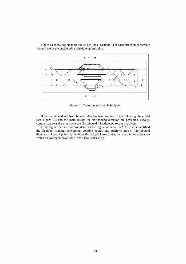
Figure 14 shows the standard routes per line at Schiphol. For each direction, 9 possible routes have been considered in schedule optimisation.

S N

S N

Figure 14: Train routes through Schiphol.

Both Southbound and Northbound traffic has been studied. In the following, the model

(see Figure 15) and the main results for Northbound direction are presented. Finally, comparison considerations between Northbound / Southbound results are given.

In the figure the external box identifies the regulation area. By “SCH” it is identified the Schiphol station, concerning possible routes and platform tracks (Northbound direction). A set of points Pi identifies the Schiphol area limits, that are the limits between which the averaged travel time in the area is measured.

23

Figure 15: The Schiphol bottleneck – Northbound direction The train characteristics considered in the model are based on data provided by

ProRail and summarised in the following table.

Table 1: Rolling stock composition Rolling stock Lenght

(m) Weight (ton)

Max speed (km/h)

TGV-P 10 200 417 220 ICE22 8 200 465 220 ICM3 6 161 287 160 IRM3 9 242 431 160 IRM4 8 214 394 160 E17D2 Dd 8 245 550 140 E17D2 Dd 6 193 459 140

In addition, TMS uses a number of detailed driving tables, describing the acceleration

and the deceleration by braking or by coasting of a certain type of train.

24

Starting from lay-out and time table models, CDR generates an optimal schedule (i.e. an optimal set of sequencing and routing decisions) whenever the involved trains enter the area. The travel times for all trains are computed according to the schedule, as train behaviour is supposed to be in fully agreement with the CDR computations. Let us recall that CDR keeps into account all the relevant network constraints and a quite precise train dynamical model, so CDR schedule can be considered very realistic, as assessed by a large amount of simulations carried out during the European projects COMBINE and COMBINE 2. A sufficient headway between trains is ensured by the choice of the alternative arc minimum length. This value was fixed to 60 seconds, leading to an average headway value of 3200 m (more than two block sections), measured between the tail of a train and the head of the subsequent one.

The complexity of the graph for Schiphol model can be indicated by the following

main quantities, related to the reference case (27 trains per hour): • # nodes: 1600

1700 • # fixed arcs: 7400 • # alternative arcs:

and by the following derived quantities: • # fixed arcs / # nodes: 1,1

4,6 • # alternative arcs / # nodes: The study considered different values of number of trains per hour (19, 23, 27, 29, 32),

starting from reference timetables provided by ProRail. In order to emulate possible degradations, two different kinds of perturbations were added to each reference timetable:

− entry delays for approaching trains (randomly sampled from a “Pearson T5” distribution)

− stop extensions at Schiphol and Hoofdoorp (randomly sampled from a normal distribution)

The entry delay disturbances depend on the entrance points, as reported in Table 2.

Table 2: distribution parameters used for the different entrance points Tab. Entrance point

(Northbound direction) p1 (average) [sec] p2 (alpha) [sec]

0 Hoofdoorp 49,5 2,3 1 Leiden/ The Hague Central Station 92,1 3,1 The Pearson T5 distribution (also known as Inverted Gamma distribution) is

characterized by a sharp peak and a slow decay. Sharpness can be tuned by the p2 (alpha) parameter, while the p1 parameter (average) acts on the position of the most probable range of values of the distribution itself.

The two distributions of entry delays for a given entrance point are reported in the following graphs:

25

Entry Delay Distribution - Tab.0

0,000

0,010

0,020

0,030

0 30 60 90 120 150 180 210 240 270 300

Seconds

Prob

abili

ty

Figure 16: distributions of entry delays for trains from Hoofdoorp

Entry Delay Distribution - Tab.1

0,000

0,010

0,020

0,030

0 30 60 90 120 150 180 210 240 270 300

Seconds

Prob

abili

ty

Figure 17: distributions of entry delays for trains from Leiden/ The Hague Central Station

The train stopping time is given by the sum of two parts: passenger time (time to get

the passengers out/in) and departing time (time to get the train ready to move). Both times are normally distributed, and the parameters depend on train type and stopping location. The selected values are listed in Table 3.

Table 3: distribution parameters used for stopping times Passenger time [sec] Departing time [sec] Station/Train Average Std. Dev. Average Std. Dev.

Hoofddorp 60 30 20 20 Shl. Stoptrains 80 30 20 20 Shl. IC’s 100 30 20 20 The total stopping time is generated by adding two random numbers drawn according

to the above distributions, and keeping into account the minimum stopping time for each train at each stopping location.

26

The random numbers are generated by starting from a given seed. A fixed number of seeds N=16 has been selected to produce the data to be averaged. Each seed produces a different realization of entry and stopping delays.

According to the above context (timetable + perturbations), a large set of different realisations was generated, each one considering 8 hours of traffic. Every 10min, CDR generated a new optimal conflict-free schedule for all the trains inside the controlled area, by acting on both precedence relations and track changes (allowed only in the Schiphol station).

Results of the Schiphol study The overall result from the study is that it is possible to manage the requested 27 trains per hour timetable through the Schiphol bottleneck, so the existing infrastructure is adequate to the objective. The result came from a relevant number of simulation hours, leading to about 2600 averaged trains for each one of the 5 analysed timetables.

From a general point of view, the study showed the benefits that can be expected from such a dynamic traffic regulation system with respect to a conventional one. The most important are:

− travel times are lower and reliability is higher. That follows from a comparison of the results produced by the CDR approach with the reference values provided by ProRail (local regulators approach), as reported in the following table.

Table 4: Computational results for the reference case 27 trains per hour Average Throughput Time [min.] Direction Reference CDR

Northbound 17,8 14,4 Southbound 17,5 15,0

− severe disturbances can be handled easier, or bad consequences of these

disturbances can be weakened. − the energy consumption is lower. − there is a better overall control of the traffic. Moreover, the CDR model can also be used to provide better timetables which allow more robust schedules. Below, the most important results of this study are reported by synthesis graphs. Average Throughput. The averaged travel time in the Schiphol area is measured

between a set of points Pi, as indicated in Figure 15. Of course, entry and exit points for a given train depend on the assigned path.

27

Average Throughput

10,011,012,013,014,015,016,017,018,019,020,021,022,023,024,0

19 23 27 29 32

Number of trains per hour

Trav

el T

ime

(min

)

Figure 18: Average Throughput Percentile Travel Time. The percentile travel time in the Schiphol area is measured

using the same data as the averaged travel time, but computing the 87th percentile of the travel time distribution. This is the travel time reachable by the 87% of the trains.

87th Percentile Throughput

12,014,016,018,020,022,024,026,028,030,032,0

19 23 27 29 32

Number of trains per hour

Trav

el T

ime

(min

)

Figure 19: 87° Percentile Throughput Exit delay. The exit delay is defined as the difference between the actual exit time and

the planned exit time, and so it measures the degree of fitting with the exit timetable.

28

Average Exit Delay

0,02,04,06,08,0

10,012,014,016,018,020,022,024,0

19 23 27 29 32

Number of trains per hour

Exi

t Del

ay (m

in)

Average

Figure 20: Average Exit Delay Punctuality. The punctuality is defined by counting how many trains have a delay less

than 3 minutes at the exit, with respect to the total number of trains. This is simply a definition, and whatever value may be use as a threshold. The choice of 3 minutes has been done in order to be conformal with the specification of the study and current practice in NL.

Figure 21: Average Punctuality The graphs show the 27 trains per hour case can be managed with reasonable

performance degradations in all the computed parameters. However, a further increase in train density is not sustainable. This is due to the

Schiphol station bottleneck where the 3 existing platforms and the approaching tracks are not sufficient to handle the traffic (with perturbations) at more than 30 trains per hour.

Northbound / Southbound comparison. Regarding average throughput, results are quite

similar for the reference case, as reported in Table 4. Considering the influence of re-routing on the quality of schedule solutions, we can see that a moderate amount of rerouting actions (10% as maximum) is sufficient to handle the perturbations in the reference case. However, inspecting the schedule solutions produced by CDR in

29

Southbound and Northbound studies, we observe a different influence of routing changes on exit delay, with respect to train orders. That happens as in Northbound direction Schiphol station is placed after the area where most conflicts occur (Hoofddorp area), whilst in Southbound it is placed before such area. So, in Northbound, most of the conflicts, detected in Hoofddorp area, are solved by changing the train orders at the confluence. Then trains approach Schiphol station in a quite proper order and routing changes are not so profitable to reduce the global exit delay. On the contrary, in Southbound direction, due to entry delays, many conflicts occur early in Schiphol station, and they are profitably solved by routing changes.

6.2 The Green Wave The pilot “The Green Wave”, actually called “de Groene Golf” (dGG), is a second application of the TMS architecture here described. The pilot was carried out in June 2004, and was a first attempt by the Strategy and Innovation Department of ProRail to test Dynamic Traffic Management (DTM) in practice.

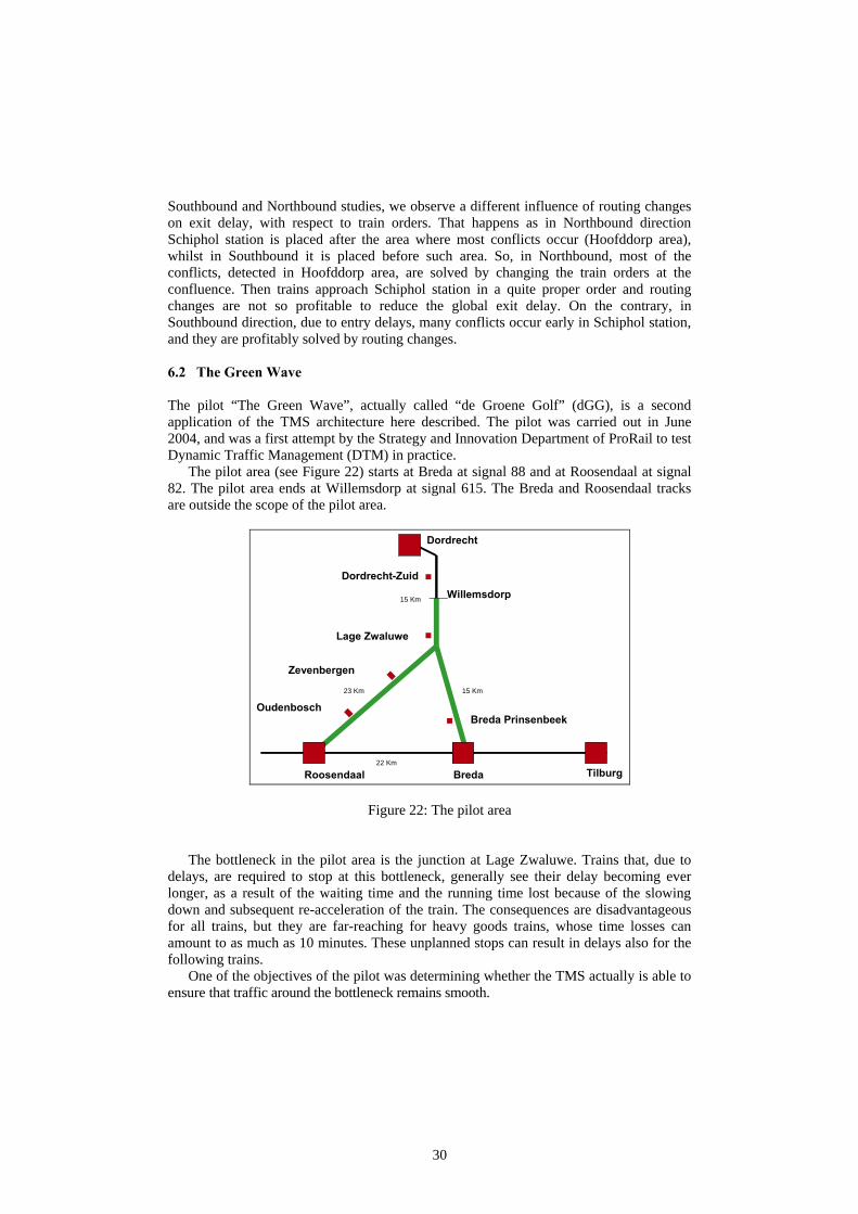
The pilot area (see Figure 22) starts at Breda at signal 88 and at Roosendaal at signal 82. The pilot area ends at Willemsdorp at signal 615. The Breda and Roosendaal tracks are outside the scope of the pilot area.

Breda Roosendaal

Dordrecht

Oudenbosch

Zevenbergen

Lage Zwaluwe

Dordrecht-Zuid

Breda Prinsenbeek

Willemsdorp

Tilburg 22 Km

23 Km 15 Km

15 Km

Figure 22: The pilot area The bottleneck in the pilot area is the junction at Lage Zwaluwe. Trains that, due to

delays, are required to stop at this bottleneck, generally see their delay becoming ever longer, as a result of the waiting time and the running time lost because of the slowing down and subsequent re-acceleration of the train. The consequences are disadvantageous for all trains, but they are far-reaching for heavy goods trains, whose time losses can amount to as much as 10 minutes. These unplanned stops can result in delays also for the following trains.

One of the objectives of the pilot was determining whether the TMS actually is able to ensure that traffic around the bottleneck remains smooth.

30

For the pilot, the TMS communicated with a Tracking & Tracing system (T&T) and the Procesleiding system (VPT-PRL). The system architecture is sketched in Figure 23.

Figure 23: System architecture The TMS received, on a regular basis, position and speed information from the

running trains, equipped by mobile units. If all trains travel according to the timetable, the influence of the TMS is minimal. The TMS then issues the timetable speed as the recommended speed. However, if there are one or more delayed trains, the TMS will calculate whether and where conflicts are set to occur.

Combining the actions of CDR and SPG, the TMS issues 3 types of recommendations, namely speed recommendations, order recommendations and route recommendations. Network controllers and train traffic controllers are the addressee of order and route recommendations. The speed recommendations are intended for the driver. By following the speed recommendations, the driver can ensure that his train is not forced to stop at a red signal. If network controllers and train traffic controllers comply with the order and route recommendations, the result is an optimum flow across the entire control area. In this way, the delay effects for other trains are minimised.

The main “quantities” of the pilot are:

• Test days: 11 8 • Pilot days:

993 • Train runs: 766 • Passenger trains:

31

211 • Freight trains: 16 • Special pilot trains: 89 • Train-attendants: 50 • Mobile units:

TMS must work in real-time, so its recommendations have to be produced as fast as

possible. This is not a problem for speed advices, as SPG computational complexity is minimal, but it can be a key aspect for order and routing recommendations, involving a new plan generation by CDR. However, being TMS core modules (CDR+SPG) installed on a dedicated PC, TMS was able to produce a new a plan in a few seconds, allowing timely reaction to perturbations.

In dGG pilot graph complexity can be indicated by the following main quantities: • # nodes: 500

600 • # fixed arcs: 600 • # alternative arcs:

and by the following derived quantities: • # fixed arcs / # nodes: 1,2

1,2 • # alternative arcs / # nodes: Comparing these indicators with the same values reported for Schiphol study, it

follows that dGG graph is simpler than Schiphol graph. Particularly the number of alternative arcs, which depends on the number of relationships between trains, is a quite small quantity in dGG graph. It depends on the topology of the pilot area, where the bottleneck is at the confluence of two separate lines. As a consequence, most train interactions are concentrated in a part of the pilot area.

Results of the pilot The effects of the TMS were demonstrated using a number of cases occurring during the pilot and analyzing the precise course of events. In some cases, it was verified that major problems caused by trains running a few minutes late, would in fact have been prevented by taking up the TMS plan and speed advices.

An example from the analysed cases is reported in the following. Starting situation This example dates from 29/06/2004 at around 09:45 hours, and describes a case

where the TMS came up with a solution for eradicating the delay, for a number of trains.

32

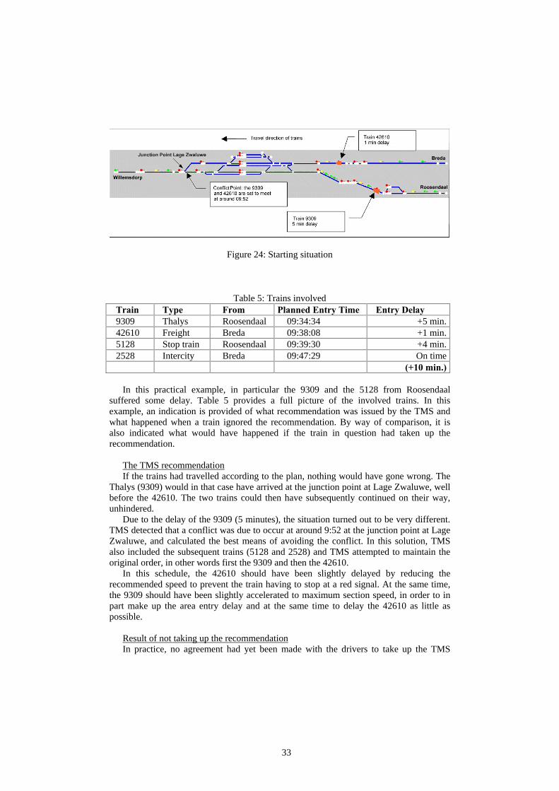
Figure 24: Starting situation

Table 5: Trains involved Train Type From Planned Entry Time Entry Delay 9309 Thalys Roosendaal 09:34:34 +5 min. 42610 Freight Breda 09:38:08 +1 min. 5128 Stop train Roosendaal 09:39:30 +4 min. 2528 Intercity Breda 09:47:29 On time

(+10 min.) In this practical example, in particular the 9309 and the 5128 from Roosendaal

suffered some delay. Table 5 provides a full picture of the involved trains. In this example, an indication is provided of what recommendation was issued by the TMS and what happened when a train ignored the recommendation. By way of comparison, it is also indicated what would have happened if the train in question had taken up the recommendation.

The TMS recommendation If the trains had travelled according to the plan, nothing would have gone wrong. The

Thalys (9309) would in that case have arrived at the junction point at Lage Zwaluwe, well before the 42610. The two trains could then have subsequently continued on their way, unhindered.

Due to the delay of the 9309 (5 minutes), the situation turned out to be very different. TMS detected that a conflict was due to occur at around 9:52 at the junction point at Lage Zwaluwe, and calculated the best means of avoiding the conflict. In this solution, TMS also included the subsequent trains (5128 and 2528) and TMS attempted to maintain the original order, in other words first the 9309 and then the 42610.

In this schedule, the 42610 should have been slightly delayed by reducing the recommended speed to prevent the train having to stop at a red signal. At the same time, the 9309 should have been slightly accelerated to maximum section speed, in order to in part make up the area entry delay and at the same time to delay the 42610 as little as possible.

Result of not taking up the recommendation In practice, no agreement had yet been made with the drivers to take up the TMS

33

recommendations. Actually, the 9309 did take up the recommendation, but the 42610 ignored it. The 42610 travelled at a speed of 65 km/hour rather than the recommended 40 km/hour. As a consequence, the 42610 was forced to stop at the red signal at the junction point at Lage Zwaluwe. The figure below shows that the Thalys was granted its route across Lage Zwaluwe (red line) whilst the 42610 had to wait for a red signal. The other two trains (2528 and 5128) are also visible in this picture.

Figure 25: 42610 at the red signal 282 The table below shows the consequences of ignoring the recommendation. Failing to

take up the speed recommendation by the 42610 resulted in a total delay of 14 minutes.

Table 6: Effects of not taking up recommendation Train Type Entry Delay Exit Delay Extra Delay 9309 Thalys +5 min. +4 min. -1 min. 42610 Freight +1 min. +7 min. +6 min. 5128 Stop train +4 min. +6 min. +2 min. 2528 Intercity On time +7 min. +7 min. (+10 min.) (+24 min.) (+14 min.)

Result if TMS recommendation had been taken up From the analysis of TMS calculation, it emerged that the above-described additional

delay would not have occurred if the 42610 had taken up the recommendation. If we assume that the Thalys in that case had also stuck to the recommendations, the 42610 would have reached the junction point several minutes later, at the recommended speed of approximately 40 km/h. As a result of which the train would not have been forced to halt for a red signal, but would have been able to pass through a green signal.

Table 3 shows the result.

Table 7: Effects of taking up recommendation Train Type Entry Delay Exit Delay Extra Delay 9309 Thalys +5 min. +4 min. -1 min. 42610 Freight +1 min. +2 min. +1 min. 5128 Stop train +4 min. +2 min. -2 min. 2528 Intercity On time +1 min. +1 min. (+10 min.) (+9 min.) (-1 min.)

Differences On balance, taking up the speed recommendation represents a gain of 15 delay

minutes. In terms of punctuality, whereby a train is only in fact delayed if the delay is

34

greater than 3 minutes, this means an output punctuality of 75% as opposed to an initial punctuality of 50%. Because in the practical situation the recommendation was not taken up, all four trains were delayed, resulting in an output punctuality of 0%.

Conclusion This example shows the strength of the TMS for improving punctuality (and the

secondary objective: saving fuel by avoiding a stop) by preventing conflicts and guiding trains on the basis of recommended speeds. The example also shows that an apparently simple problem, namely a Thalys running a few minutes late, can grow into a considerable disruption with major delays for other trains.

A global estimation of the pilot was elaborated by ProRail. This estimate is based on the analysis of a number of practical situations occurring during pilot days and on feedbacks from the involved personnel. These figures and the other experiences acquired during the trail indicate that the TMS does have sufficient capacity to become a positive addition to the existing systems. The pilot demonstrated that on a weekday, gains of approximately 210 train delay minutes could be achieved for the entire pilot area, when equipped to cover all trains. On an annual basis, the gain for the pilot could be of 1100 delay hours. The pilot has also demonstrated that the forecast energy saving of 10% is easily achieved.

In order to evaluate the personnel attitude towards TMS, a survey was sent to the train drivers and traffic controllers involved in the pilot. A usable response was received of 18 forms, representing a total of 31 journeys. Both-the train personnel and the personnel at the traffic control issued a positive judgement of the TMS system, with the footnotes that the system must be robust, and that it must be possible to easily and rapidly implement the recommendations.

7 Conclusions and Future Work

An advanced TMS addresses the problem of real-time traffic regulation and optimisation in large railway networks equipped with either fixed or moving block signalling systems. The complete TMS architecture is obtained by combining two basic concepts: decomposition of large networks in local areas, and modularity, in order to use a single approach for managing different signalling systems. In TMS, automatic local traffic optimisation and control is exploited by the complementary use of two real-time modules: • A train scheduling and routing module (CDR) • A speed regulation module (SPG

The CDR system is based on the alternative graph model, a powerful discrete optimisation model, especially designed to deal with scheduling problems where the response time is a critical factor for the evaluation of the goodness of the approach. This method is fast and detailed at the same time, and it is able to include in the optimisation model all the relevant features and constraints needed to produce efficient and realistic train scheduling solutions.

The SPG system is responsible for plan execution. Operating strictly connected to CDR, SPG computes an optimal speed profile for each train, in order to make the CDR plan being executed in a safe and energy saving manner.

Thanks to the modularity of TMS architecture, CDR can operate as stand-alone

35

module, as well as linked to SPG and other communication tools. As stand-alone tool, CDR is able to generate optimal schedules, given different traffic scenarios. The study carried out for Schiphol bottleneck 2007 suggested that the use of TMS could be effective for an efficient use of the capacity of the existing railway network and to improve reliability and punctuality of train operations.

The co-operation between CDR and SPG was put in practice in the real pilot “The Green Wave”, carried out on the Dutch track sections Roosendaal - Dordrecht and Breda - Dordrecht. The pilot showed the potential of TMS for improving train punctuality and saving fuel, by preventing conflicts and guiding trains on the basis of recommended speeds in real operations.

Currently we are working on further improvements both in TMS core functions and in TMS interfaces. Particularly, it is under investigation the use of abstract interfaces and standard formats for efficient data exchange among applications (e.g. RailML® standard in [4]). The aim is to make the TMS much more independent of the chosen implementation of the surrounding systems and more focused on the core functionalities.

References

[1] Askey S., Sheridan, T., Safety of High Speed Ground Transportation Systems - Human Factors Phase II: Design and Evaluation of Decision Aids for Control of High-Speed Trains: Experiments and Model, National Technical Information Service, Springfield, VA 22161, 1996

[2] Giannettoni M., Savio S., “The European project COMBINE 2 to improve knowledge on future rail traffic management systems”, In: Allen, J., Hill, R.J., Brebbia, C.A., Sciutto, G., Sone, S. (eds.), Computers in Railways IX, pp. 695-704, WIT Press, Southampton, 2004

[3] Giannettoni M., Savio S., “Traffic management in moving block railway systems: the results of the EU project COMBINE”, In: Allen, J., Hill, R.J., Brebbia, C.A., Sciutto, G., Sone, S. (eds.), Computers in Railways VIII, pp. 953-962, WIT Press, Southampton, 2002

[4] Huerlimann D., Nash A, Krauß V.P., Schütte J., “RailML – “A standard data interface for railroad applications”, In: Allen, J., Hill, R.J., Brebbia, C.A., Sciutto, G., Sone, S. (eds.), Computers in Railways IX, pp. 233-240, WIT Press, Southampton,.2004

[5] Kraay D. R., Harker, P. T., Real-Time Scheduling of Freight Railroads, Transportation Research Part B, 29: pp. 213-229, 1995

[6] Mascis A., Pacciarelli D., “Job shop scheduling with blocking and no-wait constraints” European Journal of Operational Research 143 (3), pp. 498-517, 2002.

[7] Mascis A., Pacciarelli,D., Pranzo, M., Models and Algorithms for traffic management of rail networks, Report DIA-74-2002, Dipartimento di Informatica e Automazione, Università Roma Tre, Roma, 2002

[8] Pellegrini F., Savio S., "Moving block and traffic management in railway applications: the EC project COMBINE", In: Allen, J., Hill, R.J., Brebbia, C.A., Sciutto, G., Sone, S. (eds.), Computers in Railways VII, pp. 11-20, WIT Press, Southampton, 2000

36