Traffic Management

1

Traffic Management

Karlsson, G., Roberts, J., Stavrakakis, I. (Eds), Alves, A., Avallone, S., Boavida, F.,D’Antonio, S., Esposito, M., Fodor, V., Gargiulo, M., Harju, J., Koucheryavy, Y., Li,F., Marsh, I., Mas Ivars, I., Moltchanov, D., Monteiro, E., Panagakis, A., Pescape, A.,

Quadros, G., Romano, S., Ventre, G.

1 Introduction

Not written yet.

2 Traffic theory and flow aware networking

We argue here that traffic theory should be increasingly used to guide the design of thefuture multiservice Internet. By traffic theory we mean the application of mathematicalmodeling to explain the traffic-performance relation linking network capacity, trafficdemand and realized performance. Traffic theoretic considerations lead us to argue thatan effective QoS network architecture must be flow aware.

Traffic theory is fundamental to the design of the telephone network. The traffic-performance relation here is typified by the Erlang loss formula which gives the prob-ability of call blocking,

�, when a certain volume of traffic, � , is offered to a given

number of circuits, � : ��

� ��

The formula relies essentially only on the reasonable assumption that telephone callsarrive as a stationary Poisson process. It demonstrates the remarkable fact that, giventhis assumption, performance depends only on a simple measure of the offered traffic,� , equal to the product of the call arrival rate and the average call duration.

We claim that it is possible to derive similar traffic-performance relations for theInternet, even if these cannot always be expressed as concisely as the Erlang formula.Deriving such relations allows us to understand what kinds of performance guaranteesare feasible and what kinds of traffic control are necessary.

It has been suggested that Internet traffic is far too complicated to be modeled usingthe techniques developed for the telephone network or for computer systems [1]. Whilewe must agree that the modeling tools cannot ignore real traffic characteristics and thatnew traffic theory does need to be developed, we seek to show here that traditionaltechniques and classical results do have their application and can shed light on theimpact of possible networking evolutions.

2

Folowing a brief discussion on Internet traffic characteristics we outline elements ofa traffic theory for the two main types of demand: streaming and elastic. We concludewith the vision of a future flow aware network architecture built on the lessons of thistheory.

2.1 Statistical characterization of traffic

Traffic in the Internet results from the uncoordinated actions of a very large populationof users and must be described in statistical terms. It is important to be able describethis traffic succinctly in a manner which is useful for network engineering.

The relative traffic proportions of TCP and UDP has varied little over at least thelast five years and tend to be the same throughout the Internet. More than 90% of bytesare in TCP connections. New streaming applications are certainly gaining in popularitybut the extra UDP traffic is offset by increases in regular data transfers using TCP. Theapplications driving these document transfers is evolving, however, with the notableimpact over recent years first of the Web and then of peer to peer applications.

For traffic engineering purposes it is not necessary to identify all the different ap-plications comprising Internet traffic. It is generally sufficient to distinguish just threefundamentally different types of traffic: elastic traffic, streaming traffic and control traf-fic. Elastic traffic corresponds to the transfer of documents under the control of TCPand is so-named because the rate of transfer can vary in response to evolving networkload. Streaming traffic results from audio and video applications which generate flowsof packets having an intrinsic rate which must be preserved by limiting packet delay andloss. Control traffic derives from a variety of signalling and network control protocols.While the efficient handling of control traffic is clearly vital for the correct operation ofthe network, its relatively small volume makes it a somewhat minor consideration fortraffic management purposes.

Fig. 1. Traffic on an OC192 backbone link.

Observations of traffic volume on network links typically reveal intensity levels (inbits/sec) averaged over periods of 5 to 10 minutes which are relatively predictable from

3

day to day (see Figure 2.1). It is possible to detect a busy period during which the trafficintensity is roughly constant. This suggests that Internet traffic, like telephone traffic,can be modelled as a stationary stochastic process. Busy hour performance is evaluatedthrough expected values pertaining to the corresponding stationary process.

The traffic process can be described in terms of the characteristics of a number ofobjects, including packets, bursts, flows, sessions and connections. The preferred choicefor modeling purposes depends on the object to which traffic controls are applied. Con-versely, in designing traffic controls it is necessary to bear in mind the facility of char-acterizing the implied traffic object. Traffic characterization proves most convenient atflow level.

A flow is defined for present purposes as the unidirectional succession of packetsrelating to one instance of an application (sometimes referred to as a microflow). Forpractical purposes, the packets belonging to a given flow have the same identifier (e.g.,source and destination addresses and port numbers) and occur with a maximum sepa-ration of a few seconds. Packet level characteristics of elastic flows are mainly inducedby the transport protocol and its interactions with the network. Streaming flows, on theother hand, have intrinsic (generally variable) rate characteristics that must be preservedas the flow traverses the network.

Flows are frequently emitted successively and in parallel in what are loosely termedsessions. A session corresponds to a continuous period of activity during which a usergenerates a set of elastic or streaming flows. For dial-up customers, the session can bedefined to correspond to the modem connection time but, in general, a session is notmaterialized by any specific network control functions.

The arrival process of flows in a backbone link typically results from the superposi-tion of a large number of independent sessions and has somewhat complex correlationbehaviour. However, observations confirm the predictable property that session arrivalsin the busy period can be assimilated to a Poisson process.

The size of elastic flows (i.e., the size of the documents transferred) is extremelyvariable and has a so-called heavy-tailed distribution: most documents are small (a fewkilobytes) but the number which are very long tend to contribute the majority of traffic.The precise distribution clearly depends on the underlying mix of applications (e.g.,mail has very different characteristics to MP3 files) and is likely to change in time asnetwork usage evolves. It is therefore highly desirable to implement traffic controls suchthat performance is largely insensitive to the precise document size characteristics.

The duration of streaming flows also typically has a heavy-tailed distribution. Fur-thermore, the packet arrival process within a variable rate streaming flow is often self-similar [2, Chapter 12]. As for elastic flows, it proves very difficult to precisely describethese characteristics. It is thus again important to design traffic controls which makeperformance largely insensitive to them.

2.2 Traffic theory for elastic traffic

Exploiting the tolerance of document transfers to rate variations implies the use ofclosed-loop control to adjust the rate at which sources emit. In this section we assumeclosed-loop control is applied end-to-end on a flow-by-flow basis using TCP.

4

TCP realizes closed loop control by implementing an additive increase, multiplica-tive decrease congestion avoidance algorithm: the rate increases linearly in the absenceof packet loss but is halved whenever loss occurs. This behavior causes each flow toadjust its average sending rate to a value depending on the capacity and the current setof competing flows on the links of its path. Available bandwidth is shared in roughlyfair proportions between all flows in progress.

A simple model of TCP results in the following well-known relationship betweenflow throughput � and packet loss rate � :

� � � � constantRTT � � �

where RTT is the flow round trip time (see [3] for a more accurate formula). This for-mula illustrates that, if we assume the loss rate is the same for all flows, bandwidth isshared in inverse proportion to the round trip time of the contending flows.

To estimate the loss rate one might be tempted to deduce the (self-similar, multi-fractal) characteristics of the packet arrival process and apply queuing theory to derivethe probability of buffer overflow. This would be an error, however, since the closed-loop control of TCP makes the arrival process dependent on the current and past conges-tion status of the buffer. This dependence is captured in the above throughput formula.

The formula can alternatively be interpreted as relating � to the realized throughput� . Since � actually depends on the set of flows in progress (each receiving a certainshare of available bandwidth), we deduce that packet scale performance is mainly de-termined by flow level traffic dynamics. It can, in particular, deteriorate rapidly as thenumber of flows sharing a link increases.

Consider the following fluid model of an isolated bottleneck link where flows arriveaccording to a Poisson process. Assume that all flows using the link receive an equalshare of bandwidth ignoring, therefore, the impact of different round trip times. Wefurther assume that rate shares are adjusted immediately as new flows begin and existingflows cease.

The number of flows in progress in this model is a random process which behaveslike the number of customers in a so-called processor sharing queue [4]. Let the linkbandwidth be � bits/s, the flow arrival rate � flows/s and the mean flow size � bits. Thedistribution of the number of flows in progress is geometric:

�� flows � � �� where

� �� is the link utilization. The expected response time � �� of a flow ofsize

�is:

� ��

� � �� From the last expression we deduce that the measure of throughput

� �� is indepen-dent of flow size and equal to � �� .

It is well known that the above results are true for any flow size distribution. It isfurther shown in [5] that they also apply with the following relaxation of the Poissonflow arrivals assumption: sessions arrive as a Poisson process and generate a finite suc-cession of flows interspersed by think times; the number of flows in the session, flow

5

sizes and think times are generally distributed and can be correlated. Statistical band-width sharing performance thus depends essentially only on link capacity and offeredtraffic.

Notice that the above model predicts excellent performance for a high capacity linkwith utilization not too close to 100%. In practice, flows handled by such links arelimited in rate elsewhere (in the access network, by a modem,...). The backbone link isthen practically transparent with respect to perceived performance.

Fig. 2. Depiction of flow throughput for 90% link load.

The above model of ideally fair bandwidth sharing usefully illustrates two inter-esting points which turn out to be more generally true. First, performance dependsprimarily on expected traffic demand (in bits/second) and only marginally on parame-ters describing the precise traffic process (distributions, correlation). Second, backboneperformance tends to be excellent as long as expected demand is somewhat less thanavailable capacity. The latter point is illustrated in Figure 2.

The figure depicts the throughput of flows traversing a bottleneck link of capacity10 Mbps under a load of 90% (i.e., flow arrival rate � average flow size = 9 Mbps), asevaluated by ns2 simulations. Flows are represented as rectangles whose left and rightcoordinates correspond to the flow start and stop time and whose height representsthe average throughput. The flow throughput is also represented by the shade of therectangle: the lightest grey corresponds to an average rate greater than 400 Kbps, blackcorresponds to less than 20 Kbps. In Figure 2, despite the relatively high load of 90%,most flows attain a high rate, as the model predicts.

In overload, when expected demand exceeds link capacity, the processor sharingqueue is unstable: the number of flows in progress increases indefinitely as flows takelonger and longer to complete while new flows continue to arrive. Figure 3 shows arectangle plot similar to Figure 2 for an offered load equal to 140% of link capacity. Therectangles tend to become black lines since the number of competing flows increasessteadily as the simulation progresses.

6

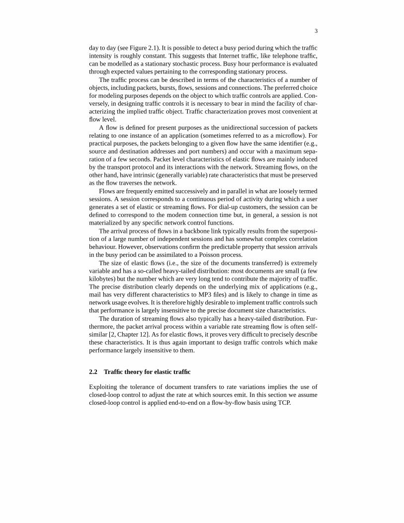
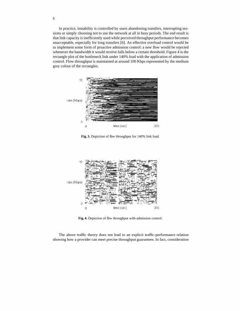
In practice, instability is controlled by users abandoning transfers, interrupting ses-sions or simply choosing not to use the network at all in busy periods. The end result isthat link capacity is inefficiently used while perceived throughput performance becomesunacceptable, especially for long transfers [6]. An effective overload control would beto implement some form of proactive admission control: a new flow would be rejectedwhenever the bandwidth it would receive falls below a certain threshold. Figure 4 is therectangle plot of the bottleneck link under 140% load with the application of admissioncontrol. Flow throughput is maintained at around 100 Kbps represented by the mediumgrey colour of the rectangles.

Fig. 3. Depiction of flow throughput for 140% link load.

Fig. 4. Depiction of flow throughput with admission control.

The above traffic theory does not lead to an explicit traffic-performance relationshowing how a provider can meet precise throughput guarantees. In fact, consideration

7

of the statistical nature of traffic, the fairness bias due to different round trip times andthe impact of slow-start on the throughput of short flows suggests that such guaranteesare unrealizable. A more reasonable objective for the provider would be to ensure a linkis capable of meeting a minimal throughput objective for a hypothetical very large flow.This throughput is equal to � � �� , even when sharing is not perfectly fair.

2.3 Traffic theory for streaming traffic

We assume that streaming traffic is subject to open-loop control: an arriving flow isassumed to have certain traffic characteristics; the network performs admission control,only accepting the flow if quality of service can be maintained; admitted flows arepoliced to ensure their traffic characteristics are indeed as assumed.

The effectiveness of open-loop control depends on how accurately performance canbe predicted given the characteristics of audio and video flows. To discuss multiplex-ing options we first make the simplifying assumption that flows have unambiguouslydefined rates like fluids. It is useful then to distinguish two forms of statistical multi-plexing: bufferless multiplexing and buffered multiplexing.

In the fluid model, statistical multiplexing is possible without buffering if the com-bined input rate is maintained below link capacity. As all excess traffic is lost, the over-all loss rate is simply the ratio of expected excess traffic to expected offered traffic, i.e.,E �� E

�� where��

is the input rate process and � is the link capacity. It isimportant to notice that this loss rate only depends on the stationary distribution of thecombined input rate but not on its time dependent properties.

The level of link utilization compatible with a given loss rate can be increased byproviding a buffer to absorb some of the input rate excess. However, the loss rate real-ized with a given buffer size and link capacity then depends in a complicated way onthe nature of the offered traffic. In particular, loss and delay performance turn out to bevery difficult to predict when the input process is self-similar (see [2, p. 540]). This isa significant observation in that it implies buffered multiplexing leads to extreme diffi-culty in controlling quality of service. Even though some applications may be tolerantof quite long packet delays it does not appear feasible to exploit this tolerance. Simpleerrors may lead to delays that are more than twice the objective or buffer overflow ratesthat are ten times the acceptable loss rate, for example.

An alternative to meeting QoS requirements by controlled statistical multiplexingis to guarantee deterministic delay bounds for flows whose rate is controlled at the net-work ingress. Network provisioning and resource allocation then relies on results fromthe so-called network calculus [7]. The disadvantage with this approach is that it typi-cally leads to considerable overprovisioning since the bounds are only ever attained inunreasonably pessimistic worst-case traffic configurations. Actual delays can be ordersof magnitude smaller.

Bufferless statistical multiplexing has clear advantages with respect to the facilitywith which quality of service can be controlled. It is also efficient when the peak rateof an individual flow is small compared to the link rate because high utilization is com-patible with negligible loss

Packet queuing occurs even with so-called bufferless multiplexing due to the coin-cidence of arrivals from independent inputs. While we assumed above that rates were

8

well defined, it is necessary in practice to account for the fact that packets in any flowarrive in bursts and packets from different flows arrive asynchronously. Fortunately, itturns out that the accumulation of jitter does not constitute a serious problem, as longas flows are correctly spaced at the network ingress [8].

Fig. 5. Bandwidth sharing between streaming and elastic flows.

Though we have discussed traffic theory for elastic and streaming traffic separately,integration of both types of flow on the same links has considerable advantages. Bygiving priority to streaming flows, they effectively see a link with very low utilizationyielding extremely low packet loss and delay. Elastic flows naturally benefit from thebandwidth which would be unused if dedicated bandwidth were reserved for streamingtraffic and thus gain greater throughput. This kind of sharing is depicted in Figure 5.

It is generally accepted that admission control must be employed for streamingflows to guarantee their low packet loss and delay requirements. Among the large num-ber of schemes which have been proposed in the literature, our preference is clearlyfor a form of measurement-based control where the only traffic descriptor is the flowpeak rate and the available rate is estimated in real time. A particularly simple schemeis proposed by Gibbens et al. [9]. In an integrated network with a majority of elastictraffic, it may not even be necessary to explicitly monitor the level of streaming traffic.

2.4 A flow aware traffic management framework

The above considerations on traffic theory for elastic and streaming flows lead us toquestion the effectiveness of the classical QoS solutions of resource reservation andclass of service differentiation [10]. In this section we outline a possible alternativeflow aware network architecture.

It appears necessary to distinguish two classes of service, namely streaming andelastic. Streaming packets must be given priority in order to avoid undue delay andloss. Bufferless multiplexing must be used to allow controlled performance of streamingflows. Packet delay and loss are then as small as they can be providing the best quality

9

of service for all applications. Bufferless multiplexing is particularly efficient under therealistic conditions that the flow peak rate is a small fraction of link capacity and themajority of traffic using the link is elastic.

Elastic flows are assumed to fairly share the residual bandwidth left by the prioritystreaming flows. From results of the processor sharing model introduced above, wededuce that the network will be virtually transparent to flow throughput as long asoverall link load is not too close to one. This observation has been confirmed by NSsimulations of an integrated system [11].

Per flow admission control is necessary to preserve performance in case demand ex-ceeds link capacity. We advocate applying admission control similarly to both streamingand elastic flows. If elastic traffic is in the majority (at least 90% at present), the admis-sion decision could be based simply on a measure of the bandwidth currently availableto a new elastic flow. If relative streaming traffic volume increases, an additional crite-rion using an estimation of the current overall streaming traffic rate could be applied asenvisaged in [9].

Implementation of flow aware networking obviously requires a reliable means ofidentifying individual flows. A flow identifier could be derived from the usual microflow5-tuple of IPv4. A more flexible solution would be to use the flow label field of the IPv6packet header allowing the user to freely define what he considers to constitute a ‘flow’(e.g., all the elements of a given Web page).

Flow identification for admission control would be performed ‘on the fly’ by com-paring the packet flow identifier to a list of flows in progress on a controlled link. If thepacket corresponds to a new flow, and the admission criteria are not satisfied, the packetwould be discarded. This is a congestion signal to be interpreted by the user, as in theprobe-based admission schemes discussed in Section XX. If admissible, the new flowidentifier is added to the list. It is purged from the list when no packet is observed in acertain timeout interval.

Admission control preserves the efficiency of links whose demand exceeds capac-ity. Rather than rejecting excess flows, a more satisfactory solution would be to choosean alternative route. This constitutes a form of adaptive routing and would consider-ably improve network robustness and efficiency compared to that currently offered byInternet routing protocols.

Admission control can be applied selectively depending on a class of service associ-ated with the flow. Regular flows would be rejected at the onset of congestion, premiumflows only if congestion even then degrades to some higher degree. This constitutes aform of service differentiation with respect to accessibility.

Note finally that all admitted flows have adequate quality of service and are there-fore subject to charging. A simple charging scheme is appropriate based on byte count-ing without any need to distinguish different service classes: streaming flows experiencenegligible packet loss and delay while elastic flows are guaranteed a higher overallthroughput.

10

3 An IP Service Model for the Support of Traffic Classes

3.1 Introduction

The project that led to the development of the IP service model presented in this textstarted with the development of a metric for evaluating the quality of service in packetswitched networks. Such a metric, presented in [12] and hereafter named QoS metric,is aimed at measuring quantifiable QoS characteristics [13] in communication systems,as throughput, transit delay or packets loss. It is especially tailored to the intermediarylayers of communication systems, namely the network layer. During the metric develop-ment some ideas arose and were subsequently refined, progressively leading to a novelIP service model.

The central idea behind the proposed model is still to treat the traffic using theclassical best effort approach, but with the traffic divided into several classes insteadof a single class. This corresponds to a shift from a single-class best-effort paradigmto a multiple-class best-effort paradigm. In order to do this, a strategy which dynami-cally redistributes the communication resources is adopted, allowing classes for whichdegradation does not cause a significant impact to absorb the major part of congestion,thereby relieving the remaining classes.

Classes are characterized by traffic volumes, which can be potentially very different,and can be treated better or worse inside the communication system according to theirneeds and to the available resources. This means that classes may suffer better or worseloss levels inside the network and their packets may experience bigger or smaller transitdelays. The model’s capacity to differentiate traffic is achieved by controlling the transitdelay and losses suffered by packets belonging to different classes, through the dynamicdistribution of processing and memory resources. The bandwidth used by the traffic isnot directly controlled, because the characteristics of the model make it unnecessary.

3.2 Service Model

The model proposal discussed here follows the differentiated services architecture [14]and considers that traffic is classified into classes according to its QoS needs. The cen-tral idea is still to treat the traffic using the best effort approach, but with the trafficdivided into several classes instead of a single one. Thus, traffic is still treated as wellas possible, but that now means different things according to the considered class.

In order to do that, a strategy is adopted which dynamically redistributes the com-munications resources, allowing classes for which degradation does not have a signifi-cant impact to absorb the major part of it, thereby relieving the remaining ones.

The model’s capacity to differentiate traffic is achieved by controlling the transitdelay and losses suffered by packets of the different classes (which is the goal of thedynamic distribution of resources). The bandwidth used by the traffic is not controlled.Given the characteristics of the model, this kind of control is not necessary (and notpossible either).

In fact, as one of the main goals of the model is to avoid complexity, traffic spec-ifications and explicit resource reservations are not considered. As a result, it is notpossible to anticipate the bandwidth used by the different classes and, consequently, it

11

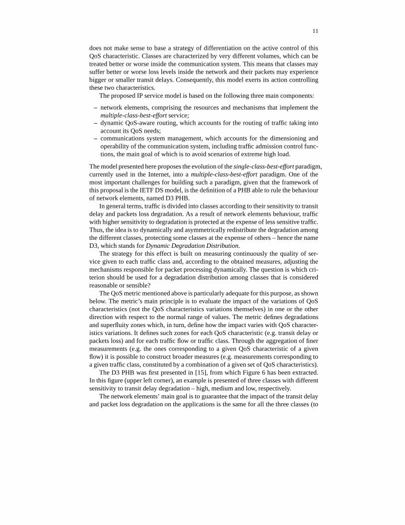
does not make sense to base a strategy of differentiation on the active control of thisQoS characteristic. Classes are characterized by very different volumes, which can betreated better or worse inside the communication system. This means that classes maysuffer better or worse loss levels inside the network and their packets may experiencebigger or smaller transit delays. Consequently, this model exerts its action controllingthese two characteristics.

The proposed IP service model is based on the following three main components:

– network elements, comprising the resources and mechanisms that implement themultiple-class-best-effort service;

– dynamic QoS-aware routing, which accounts for the routing of traffic taking intoaccount its QoS needs;

– communications system management, which accounts for the dimensioning andoperability of the communication system, including traffic admission control func-tions, the main goal of which is to avoid scenarios of extreme high load.

The model presented here proposes the evolution of the single-class-best-effort paradigm,currently used in the Internet, into a multiple-class-best-effort paradigm. One of themost important challenges for building such a paradigm, given that the framework ofthis proposal is the IETF DS model, is the definition of a PHB able to rule the behaviourof network elements, named D3 PHB.

In general terms, traffic is divided into classes according to their sensitivity to transitdelay and packets loss degradation. As a result of network elements behaviour, trafficwith higher sensitivity to degradation is protected at the expense of less sensitive traffic.Thus, the idea is to dynamically and asymmetrically redistribute the degradation amongthe different classes, protecting some classes at the expense of others – hence the nameD3, which stands for Dynamic Degradation Distribution.

The strategy for this effect is built on measuring continuously the quality of ser-vice given to each traffic class and, according to the obtained measures, adjusting themechanisms responsible for packet processing dynamically. The question is which cri-terion should be used for a degradation distribution among classes that is consideredreasonable or sensible?

The QoS metric mentioned above is particularly adequate for this purpose, as shownbelow. The metric’s main principle is to evaluate the impact of the variations of QoScharacteristics (not the QoS characteristics variations themselves) in one or the otherdirection with respect to the normal range of values. The metric defines degradationsand superfluity zones which, in turn, define how the impact varies with QoS character-istics variations. It defines such zones for each QoS characteristic (e.g. transit delay orpackets loss) and for each traffic flow or traffic class. Through the aggregation of finermeasurements (e.g. the ones corresponding to a given QoS characteristic of a givenflow) it is possible to construct broader measures (e.g. measurements corresponding toa given traffic class, constituted by a combination of a given set of QoS characteristics).

The D3 PHB was first presented in [15], from which Figure 6 has been extracted.In this figure (upper left corner), an example is presented of three classes with differentsensitivity to transit delay degradation – high, medium and low, respectively.

The network elements’ main goal is to guarantee that the impact of the transit delayand packet loss degradation on the applications is the same for all the three classes (to

12

facilitate the presentation let us consider for now transit delay only). Therefore, networkelements must control the transit delay suffered by packets of the three different classesin such a way that the congestion indexes related to this QoS characteristic are the samefor all classes. Considering again Figure 6 as a reference, suppose that for a certain loadlevel, which happens in the instant of time t1, this impact is evaluated by the index valueCI��

. Then, the transit delays suffered by the packets of each class are, from the most tothe least sensitive, d1, d2 and d3, respectively.

Fig. 6. Congestion indexes for three traffic classes with different sensitivity to delay degradation.

In a more formal manner, the above mentioned goal means that the following equa-tion holds for any time interval [t

�, t��]:

��

� � � � � ��

� � � (1)

Exactly the same reasoning should be made if packet losses, instead of transit delay,are used as the QoS characteristic for evaluating the degradation of quality of service.In this case the formula which applies to any time interval [t

�, t��] is the following:

�� "! �� "! ��

� � � � � �� "! ��

� � �� "! �� (2)

Thus, equations 1 and 2 establish the formal criterion which rules the network ele-ments’ behaviour in respect to the way IP packets are treated. Through its simultaneousapplication, network elements control, in an integrated way, the transit delay and losslevel suffered by the different classes.

13

To understand the way traffic from classes more sensitive to degradation is, in fact,protected from less sensitive traffic, let us consider again Figure 7. Its upper left cornerrepresents a load situation that corresponds, as seen before, to a congestion index equalto CI

��.

Suppose that at a given instant of time, t2, the load level to which the network ele-ment is submitted, rises. The impact of the degradation felt by the different applications(which generate traffic for the different classes) will also rise. The mechanisms of thenetwork element will adjust themselves taking into account the criterion for resourcedistribution, that is, the values of such an impact (the congestion indexes) must be equalfor all the classes. As can be seen in Figure 7 (right side), this corresponds to transit de-lays from the most to the least sensitive class of d’1, d’2 and d’3, respectively.

It is possible to see clearly in the figure that the value of (d’1-d1) is lower than thevalue of (d’2-d2) which, in turn, is lower than the value of (d’3-d3). Thus, the increasein transit delay suffered by packets of the different classes, when the load grows, islower for classes that are more sensitive to transit delay degradation and greater forless sensitive classes. Hence, the degradation that happened at t2 was asymmetricallydistributed among the different classes, the major part of it being absorbed by the onesless sensitive to degradation. Summing up, more sensitive classes are in fact protectedat the expense of less sensitive classes, which is one of the most important goals of thisproposal.

Finally, it is important to say that the control of the way in which some classes areprotected at the expense of others, or even of the degradation part effectively absorbedby less sensitive classes, is materialized through the definition of the degradation sen-sitivity for each class (or, which is the same, through the definition of the size of eachdegradation zone).

3.3 An implementation of the D3 per-hop behaviour

It order to test the ideas put forward in the proposed IP service model, it was decided tobuild a prototype of the D3 PHB. This section describes this prototype.

The packet scheduler The basic idea of the work described in this section was the in-tegration of the characteristics of the work-conserving (WC) and non-work-conserving(NWC) disciplines in one single mechanism, in order to obtain a new packet scheduler,which was simple but very functional – considering the characteristics of the PHB itwould have to support – and able to effectively overcome the difficulties revealed bythe experiments referred to in the previous sub-section.

Such a scheduler was first described in [16]. Figure 7 – extracted from that paper –presents the logical diagram of the scheduler. This figure shows the scheduler organisedinto two modules that reflect two stages of the controller’s development.

Taking DEQUEUE TIME as the instant of time after which the controller may pro-cess the next packet in a certain queue, XDELAY as the period of time that must passbetween the processing of two consecutive packets in a certain queue (that is to say, theminimum time that a packet must wait in its queue), and TEMPO as the current systemtime, this is, concisely, how the scheduler works:

14

Fig. 7. Logical diagram of the scheduler implemented at LCT.

– it sequentially visits (round-robin) each IP queue, meaning, each class;– on each visit it compares TEMPO against the value of the variable DEQUEUE TIME

that characterises the queue; if the first is greater than the second, the packet at thehead of the queue is processed;

– on each visit it updates, if necessary, the queue’s DEQUEUE TIME (which is doneby adding the value of the variable XDELAY1 to TEMPO);

– for the most important class (the reference class), XDELAY is zero, which meansthat the scheduler behaves as a WC one. For all the other classes XDELAY will begreater than zero and will reflect the relative importance of each class. In this way,in these cases, the controller behaves as a NWC controller.

The packet dropper Having developed the packet scheduler, the next challenge be-came the conception of an integrated solution to control the loss of packets. In this textit has been referred to as the packet dropper (as opposed to the packet scheduler). Inreality, the construction of the model demands far more that one packet dropper. It de-mands an active queue management strategy that allows not only an intelligent drop ofthe packets to be eliminated, but also an effective control of the loss level suffered bythe different classes (without this, the operational principle of equality of the congestionindexes related to losses cannot be accomplished).

The queue management system was first presented in [17]. In general terms, thepresent system involves the storing of packets in queues and their discarding when nec-essary. It is composed of two essential modules – the queue length management module(QLMM) and the packet drop management module (PDMM) � The network element’sgeneral architecture, including the queue management system and the packet scheduler,is presented in Figure 8.

1 X DELAY means the time, in � s, that the packet must wait in its queue.

15

Fig. 8. Network element’s general architecture [15].

3.4 Tests made to the D3 PHB implementation

The tests made to the D3 implementation can be subdivided into three main groups:robustness tests, performance tests and functional tests. During the development of thework presented here, tests pertaining to each of these groups were carried out.

The tests were carried out using both the QoStat tool [18] and netiQ’s Chariot tool[19]. QoStat is a graphical user interface tool with the following characteristics:

– Graphical and numerical real-time visualisation of all values pertaining to the pro-vision of quality of service by network elements, such as transit delay, number ofprocessed packets, number of dropped packets per unit of time, queues’ length, andused bandwidth.

– On the fly modification of all QoS-related operational parameters of network ele-ments, such as maximum queue lengths, WFQ/ALTQ queue weights, virtual andphysical queue limits, sensitivity of classes to delay degradation, and sensitivity ofclasses to loss degradation.

The tests made to the packet scheduler whose objective was to perform a first evaluationof the differentiation capability of the prototype, clearly showed the effectiveness of thescheduler. The tests’ description and their results are presented in [16].

One example is the test carried out over a small isolated network composed oftwo source hosts independently connected through a router (with the new schedulerinstalled) to a destination host. All the hosts were connected through 100 Mbps FastEthernet interfaces and configured with queues with a maximum length of 50 packets.Two independent UDP flows composed of 1400 bytes packets were generated at the

16

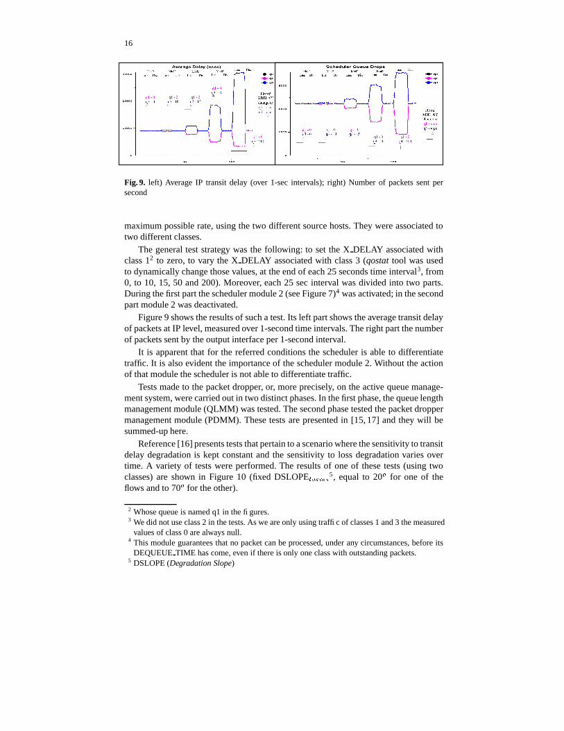
Fig. 9. left) Average IP transit delay (over 1-sec intervals); right) Number of packets sent persecond

maximum possible rate, using the two different source hosts. They were associated totwo different classes.

The general test strategy was the following: to set the X DELAY associated withclass 12 to zero, to vary the X DELAY associated with class 3 (qostat tool was usedto dynamically change those values, at the end of each 25 seconds time interval3, from0, to 10, 15, 50 and 200). Moreover, each 25 sec interval was divided into two parts.During the first part the scheduler module 2 (see Figure 7)4 was activated; in the secondpart module 2 was deactivated.

Figure 9 shows the results of such a test. Its left part shows the average transit delayof packets at IP level, measured over 1-second time intervals. The right part the numberof packets sent by the output interface per 1-second interval.

It is apparent that for the referred conditions the scheduler is able to differentiatetraffic. It is also evident the importance of the scheduler module 2. Without the actionof that module the scheduler is not able to differentiate traffic.

Tests made to the packet dropper, or, more precisely, on the active queue manage-ment system, were carried out in two distinct phases. In the first phase, the queue lengthmanagement module (QLMM) was tested. The second phase tested the packet droppermanagement module (PDMM). These tests are presented in [15, 17] and they will besummed-up here.

Reference [16] presents tests that pertain to a scenario where the sensitivity to transitdelay degradation is kept constant and the sensitivity to loss degradation varies overtime. A variety of tests were performed. The results of one of these tests (using twoclasses) are shown in Figure 10 (fixed DSLOPE � ! �� 5, equal to 20

!for one of the

flows and to 70!

for the other).

2 Whose queue is named q1 in the figures.3 We did not use class 2 in the tests. As we are only using traffic of classes 1 and 3 the measured

values of class 0 are always null.4 This module guarantees that no packet can be processed, under any circumstances, before its

DEQUEUE TIME has come, even if there is only one class with outstanding packets.5 DSLOPE (Degradation Slope)

17

Fig. 10. Tests results in the following scenario: fixed DSLOPElosses, equal to 20� for the q2 flowand to 70 � for the q1 flow; delay sensitivity varied over time.

It is possible to observe that, under these conditions, the behaviour is as expected.The number of packets that get processed per unit of time, which is a complement ofthe number of dropped packets per unit of time, is constant and consistent with therespective loss class sensitivity, DSLOPE � ! �� . This happened in spite of the fact thattransit delay was made to vary over time.

3.5 Conclusions and further work

One of the main objectives of the work presented in this paper was the conception ofan IP service model based on the so called multiple-class-best-effort (mc-be) paradigm.This model is intended to deal with traffic classes taking into account their specific QoSneeds, while still treating them as well as possible (without leaving aside the actual IPtechnology).

The applications do not have to specify the characteristics of the traffic they gener-ate, nor explicitly request the QoS levels they need. Under heavy load conditions in thecommunication system (i.e. when performance degradation is likely to happen), theyreceive a better or worse treatment according to the traffic class they have chosen. Thisreflects the sensitivity to degradation pre-configured for each class, namely, the trafficsensitivity to delay degradation and the traffic sensitivity to the degradation of the levelof packet losses.

The work presented here has strategically focused on the network element. This wasachieved through the conception of a Per Hop Behaviour (PHB) capable of supportingthe referred to model (the D3 PHB – Dynamic Degradation Distribution), and by theconstruction of the respective prototype.

The tests carried out on the prototype showed a very promising behaviour withregard to its capacity for differentiating the treatment applied to the classes in a coher-ent and controllable way. However, in order to characterise and evaluate the presentedmodel in a more precise manner, it is clear that the prototype must be further tested, us-ing network load conditions closer to those which actually happen inside IP networks.The development of other components of the model also fits into future work, namely,

18

the development of the QoS-based routing component and the traffic admission controlcomponent which, as referred to above, are currently being developed at the LCT-UC[20–22].

Meanwhile, there is a set of contributions that stand out, as results of the work pre-sented in this text: (1) a metric for the evaluation of QoS in IP networks; (2) an IPservice model that supports the mc-be paradigm; (3) a PHB that supports the model,specifically considering the network element – the D3 PHB; (4) an implementation ofsuch a PHB model involving the building of a packet scheduler and a queuing manage-ment system, which work together towards the D3 purposes.

4 Probe–based admission control in IP networks

4.1 Introduction

Today’s new applications on the Internet require a better and more predictable ser-vice quality than what is possible with the available best–effort service. Audio-visualapplications can handle limited packet loss and delay variation without affecting theperceived quality. Interactive communication in addition requires stringent delay re-quirements. For example, IP telephony requires roughly speaking a maximum of 150ms one–way delay that needs to be kept during the whole call.

The question of whether to provide the required service quality by over–provisioningnetwork resources, or by admission control and reservation schemes, has been dis-cussed extensively in the last years. In [23], Breslau and Shenker compare networkperformance and cost with over–provisioning and reservation. Considering non–elasticapplications, their analysis shows that the amount of incremental capacity needed toobtain the same performance with a best–effort network as with a reservation–capablenetwork diverges as capacity increases. Reservation retains significant advantages insome cases over over–provisioning, no matter how inexpensive the capacity becomes.Consequently, efficient reservation schemes can play an important role in the futureInternet.

The IETF has proposed two different approaches to provide quality of service guar-antees: Integrated Services (IntServ) [24] and Differentiated Services (DiffServ) [25].IntServ provides three classes of service to the users: The guaranteed service (GS) of-fers transmission without packet loss and bounded end-to-end delays by assuring afixed amount of capacity for the traffic flows [26]; the controlled load service (CLS)provides a service similar to a best–effort service in a lightly loaded network by pre-venting network congestion [27]; and, finally, the best–effort service lacks any kind ofQoS assurances.

In the IntServ architecture, GS and CLS flows have to request admission from thenetwork using the resource reservation protocol RSVP [28]. RSVP provides unidirec-tional per–flow resource reservations. When a sender wants to start a new flow, it sendsa path message to the receiver. The message traverses all the routers in the path to the re-ceiver, which replies with a resv message indicating the resources needed at every hop.This resv message can be denied by any router in the path, depending on the availabilityof resources. When the sender receives the resv message, the network has reserved the

19

required resources along the transmission path and the flow is admitted. IntServ routersthus need to keep per–flow states and must process per–flow reservation requests, whichcan create an unmanageable processing load in the case of many simultaneous flows.Consequently, the IntServ architecture provides excellent quality in the GS class, andtight performance bounds in the CLS class, but has known scalability limitations.

The second approach for providing QoS in the Internet, the DiffServ architecture,puts much less burden on the routers, thus providing much better scalability. DiffServuses an approach referred to as class of service (CoS), by mapping multiple flows intotwo default classes. Applications or ingress nodes mark packets with a DiffServ codepoint(DSCP) according to their QoS requirements. This DSCP is then mapped intodifferent per–hop behaviors (PHB) at each router on the path, like expedited forward-ing [29], or assured forwarding [30]. The routers additionally provide a set of priorityclasses with associated queues and scheduling mechanisms, and they schedule packetsbased on the per–hop behavior.

The drawback of the DiffServ scheme is that as it does not contain admission con-trol. The service classes may be overloaded and all the flows belonging to that classmay suffer increased packet loss. To handle overload situations, DiffServ relies on ser-vice level agreements (SLA) between DiffServ domains, which establish the policycriteria, and define the traffic profiles. Traffic is policed and smoothed at ingress pointsaccording to the SLA. Traffic that is out of profile (i.e. above the upper bounds of ca-pacity usage stated in the SLA) at an ingress point has no guarantees and can be eitherdropped, over charged, or downgraded to a lower QoS class. Compared to the IntServsolution, DiffServ improves scalability at the cost of a less predictable service to userflows. Moreover, DiffServ eliminates the possibility to change the service requirementsdynamically by the end user, since it would require signing a new SLA. Thus providingof quality of service is almost static.

Both IETF schemes provide end–to–end QoS with different approaches and thuswith different advantages and drawbacks. Recent efforts focus on combining both schemes,like RSVP aggregation [31], the RSVP DCLASS object [32], or the proposal of the in-tegrated services over specific link layer working group (ISSLL) to provide IntServ overDiffServ networks [33], that builds on RSVP as signaling protocol but uses DiffServ toactually share the resources among the flows.

4.2 Per–hop Measurement Based Admission Control Schemes

Recently, a set of measurement–based admission control schemes has appeared in theliterature. These schemes follow the ideas of IntServ, with connection admission controlalgorithms to limit network load, but without the need of per–flow states and exacttraffic descriptors. They use some worst–case traffic descriptor, like the peak rate, todescribe flows trying to enter the network, and then to base the acceptance decision ineach hop on real–time measurements of the individual or aggregate flows.

All these algorithms focus on provisioning resources at a single network node andfollow some admission policy, like complete partitioning or complete sharing. The com-plete partitioning scheme assumes a fixed partition of the link capacity for the differentclasses of connections. Each partition corresponds to a range of declared peak rates,and the partitions cover together the full range of allowed peak rates without overlap.

20

A new flow is admitted only if there is enough capacity in its class partition. This pro-vides a fair distribution of the blocking probability amongst the different traffic classes,but it risks lowering the total throughput if some classes are lightly loaded while oth-ers are overloaded. The complete sharing scheme, on the contrary, makes no differenceamong flows. A new flow is admitted if there is capacity for it, which may lead to adominance of flows with smaller peak rate. To perform the actual admission control,measurement–based schemes use RSVP signaling.

The idea of measurement based admission control is further simplified in [34]. Inthis proposal the edge routers decide about the admission of a new flow. Edge routerspassively monitor the aggregate traffic on transmission paths, and accept new flowsbased on these measurements.

An overview of several MBAC schemes is presented in [35]. This overview revealsthat all the considered algorithms have similar performance, independently of their al-gorithmic complexity. While measurement–based admission control schemes requirelimited capabilities from the routers and source nodes, compared to traditional admis-sion control or reservation schemes, like RSVP, they show a set of drawbacks: Not allproposed algorithms can select the target loss rate freely, flows with longer transmis-sion paths experience higher blocking probabilities than flows with short paths, andflows with low capacity requirements are favored over those with high capacity needs.

4.3 Endpoint Admission Control Schemes

In the recent years a new family of admission control solutions has been proposedto provide admission control for controlled–load like services, with very little or nosupport from routers. These proposals share the common idea of endpoint admissioncontrol: A host sends probe packets before starting a new session and decides aboutthe flow admission based on statistics of probe packet loss [36, 37], explicit congestionnotification (ECN) marks [38–40], delay or delay variation [41–43]. The admissiondecision is thus moved to the edge nodes, and it is made for the entire path from thesource to the destination, rather than per–hop. Consequently, the service class doesnot require explicit support from the routers, other than one of the various schedulingmechanisms supplied by DiffServ, and possibly the capability of marking packets.

In most of the schemes the accuracy of the probe process requires the transmissionof a large number of probe packets to provide measurements with good confidence.Furthermore, the schemes require a high multiplexing level on the links to make surethat the load variations are small compared to the average load.

A detailed comparison of the different endpoint admission control proposals is givenin [44], showing that the performance of the different admission control algorithmsis quite similar, and thus the complexity of the schemes may be the most importantdesign consideration. The following sections briefly summarize the three main sets ofproposals.

Admission control based on probe loss statistics In the proposal from Karlsson etal. [36, 37, 45, 46] the call admission is decided based on the experienced packet lossduring a short probe phase, ensuring that the loss ratio of accepted flows is bounded.

21

Delay and delay jitter are limited by using small buffers in the network. Probe packetsand data packets of accepted flows are transmitted with low and high priority respec-tively, to protect accepted flows from the load of the probe streams. The probing is doneat the peak rate of the connection and the flow is accepted if the probe packet loss rateis below a predefined threshold. This procedure ensures that the packet loss of acceptedflows is always below the threshold value.

Admission control based on ECN marks The congestion level in the network in theproposal from F. Kelly et al. [39] and T. Kelly [40] is determined by the number ofprobe packets received with ECN marks by the end host. In this case, probe packetsare transmitted together with data packets. To avoid network overload caused by theprobes themselves the probing is done incrementally in probe rounds that last approx-imately one RTT, up to the peak rate of the incoming call. ECN–enabled routers onthe transmission path set the ECN congestion experienced bit when the router detectscongestion, e.g., when the buffer content exceeds a threshold or after a packet loss [38].The call is accepted if the number of marked packets is below a predefined value. Thisproposal suggests that by running appropriate end–system response to the ECN marks,a low delay and loss network can be achieved.

The call admission control is coupled with a pricing scheme [47]. In this case usersare allowed to send as much data as they wish, but they pay for the congestion theycreate (the packets that are marked). In this congestion pricing scheme the probing pro-tocol estimates the price of a call, that is compared with the amount the end–system iswilling to pay. The scheme does not provide connections with hard guarantees of ser-vice; it merely allows connections to infer whether it is acceptable to enter the networkor not.

Admission control based on delay variations Bianchi et al. [43, 48] (first versionpublished in [42]) propose to use measurements on the variation of packet inter–arrivaltime to decide about call admission, based on the fact that a non–negligible delay jittercan be observed even for accepted loads well under the link capacity. The admissioncontrol is designed to support IP telephony, thus it considers low and constant bit rateflows. The probe packets are sent at a lower priority than data packets. The probingphase consists of the consecutive transmission of a number of probe packets with afixed inter–departure time. A maximum tolerance on the delay jitter of the receivedprobe packets is set at the receiving node, and the flow is rejected immediately if thecondition fails for one probe packet. The maximum tolerance on the delay jitter and thenumber of probe packets transmitted regulates the maximum level of accepted load onthe network links. This maximum load is selected in a way such that the packet lossprobability and end–to–end delay requirements for the accepted calls are met.

4.4 PBAC: Probe–Based Admission Control

As an example, we discuss the endpoint admission control procedure based on packetloss statistics in detail [36, 37, 45, 46]. This solution offers a reliable upper bound on

22

the packet loss for the accepted flows, while it limits the delay and delay jitter by theuse of small buffers in the routers.

The admission control is done by measuring the loss ratio of probe packets sent atthe peak rate of the flow and transmitted with low priority at the routers. The schedulingsystem of the routers consequently has to differentiate data packets from probe packets.To achieve this, two different approaches are possible. In the first one there are twoqueues, one with high priority for data and one with low priority for probe packets (seeFigure 11). In the second approach, there is just one queue with a discard threshold forthe probes. Considering the double–queue solution the size of the high priority bufferfor the data packets is selected to ensure a low maximum queuing delay and an accept-able packet loss probability, i.e., to provide packet scale buffering [49]. The buffer forthe probe packets on the other hand can accommodate one packet at a time, to ensurean over–estimation of the data packet loss. The threshold–queue can be designed toprovide similar performance, as it is shown in [45], and the choice between the twoapproaches can be left as a decision for the router designer.

Figure 12 shows the phases of the PBAC session establishment scheme. When a hostwishes to set up a new flow, it starts by sending a constant bit rate probe at the maximumrate the data flow will require. The probing time is chosen by the sender from a rangeof values defined in the service contract. This range forces new flows to probe for asufficient time to obtain a sufficiently accurate measurement, while it prohibits themfrom performing unnecessarily long probes. The probe packet size should be smallenough so that there are sufficient number of packets in the probing period to performthe acceptance decision. When the host sends the probe packets, it includes the peakbit rate and the length of the probe, as well as a packet and flow sequence number inthe data field of each packet. With this information the end host can perform an earlyrejection, based on the expected number of packets that it should receive not to surpassthe target loss probability. The probe contains a flow identifier to allow the end host todistinguish probes for different sessions. Since one sender could open more than onesession simultaneously, the IP address in the probes is not enough to differentiate them.When the probe process finishes, the sender starts a timer with a value over two timesthe expected round trip time. This timer goes off in case the sender does not receivean acknowledgement to the probe. The timer allows the sender to infer that none ofthe probe packets went through or the acknowledgement packet with the acceptancedecision from the receiver got lost. The sender assumes the first scenario and backs offfor a long period of time, still waiting for a possible late acknowledgement. In case a lateacknowledgement arrives the sender acts accordingly and cancels the backoff process.

Upon receiving the first probe packet for a flow, the end host starts counting thenumber of received packets and the number of lost packets (by checking the sequencenumber of the packets it receives). When the probing period finishes and the end hostreceives the last probe packet, it compares the probe loss measured with the target lossand sends back an acknowledgement packet accepting or rejecting the incoming flow.This acknowledgement packet is sent back at high priority to minimize the risk of loss.If the decision is positive, the receiver starts a timer to control the arrival of data packets.The value of this timer should be slightly more than two RTTs. If this timer goes off,the host assumes that the acceptance packet has been lost and resends it.

23

8

Packet Buffers

8

Packet Buffers

Threshold2 packets

Data

Probes+ Low + High

priority

Highpriority

Lowpriority

Low + Highpriority

Threshold QueueScheme

Double QueueSchemePacket Buffers

2Probes

Data

The queueing scheme of the CLS

Fig. 11. The queueing system.

ACK

ACK

newsession

newsession

newsession

NACK

Probe

Probe

Probe

Probe

ACK

Data

Data

Data

MeasurementProbe length

Ploss < Ptarget

MeasurementProbe length

Ploss < Ptarget

Backofftime

Probe length

Measurement

Measurement

Probe length

Ploss < Ptarget

Ploss > Ptarget

Tim

eout

Tim

eout

Tim

eout

Tim

eout

Tim

eout

Tim

eout

Tim

eout

Fig. 12. The probing procedure.

Finally, when the sending host receives the acceptance decision, it starts sendingdata with high priority, or, in the case of a rejection, it backs off for a certain amountof time, before starting to probe again. In subsequent tries, the sender host can increasethe probe length, up to the maximum level allowed, so that a higher accuracy on themeasurement is achieved. There is a maximum number of retries that a host is allowed toperform before having to give up. The back off strategy and the number of retries affectthe connection setup time for new sessions and should be carefully tuned to balance theacceptance probability with the expected setup delay.

The acceptance threshold is fixed for the service class and is the same for all ses-sions. The reason for this is that the QoS experienced by a flow is a function of theload from the flows already accepted in the class. Considering that this load dependson the highest acceptance threshold among all sessions, by having different thresholdsall flows would degrade to the QoS required by the one with the less stringent require-ments. The class definition also has to state the maximum data rate allowed to limit thesize of the sessions that can be set up. Each data flow should not represent more than asmall fraction of the service class capacity (in the order of 1%), to ensure that statisticalmultiplexing works well.

A critical aspect of end–to–end measurement based admission control schemes isthat the admission procedure relies on common trust between the hosts and the network.If this trust is not present, security mechanisms have to protect the scheme. First, asend hosts decide about the admission decision based on measurements performed inthe network, their behavior has to be monitored to avoid resource misuse. Second, asinformation on the call acceptance has to be transmitted from the receiving node tothe source, intruder attacks on the transmission path altering this information have tobe avoided. The specific security mechanisms of the general end–to–end measurementbased admission control schemes can be addressed in different ways that are out of thescope of this overview, but a simple cryptographic scheme has been proposed in [50].

Application to Multicast A solution to extend the idea of end-to-end measurementbased admission control for multicast communication is presented in [46]. The pro-

24

posed scheme builds on the unicast PBAC process. The admission control procedureassumes a sender–based multicast routing protocol with a root node (rendez-vous point)implemented. The root node of the multicast tree takes active part in the probing processof the admission control, while the rest of the routers only need to have the priority–based queueing system to differentiate probes and data, as in the original unicast PBACscheme.

In order to adapt the admission control for multicast communication two multicastgroups are created: one for the probe process and one for the data session itself. Sendersfirst probe the path until the root node of the multicast tree, and start to send data ifaccepted by this node. The probe from the sender is continuously sent to the root node,and is forwarded along the multicast tree of the probe group whenever receivers havejoined this group.

Receivers trying to join the multicast data group first join the probe group to performthe admission control. They receive the probe packets sent by the sender node andforwarded by the root node, and decide about the admission based on the packet lossratio. If the call is accepted the receiver leaves the probe group and joins the data group.Consequently, receivers have to know the addresses of both the probe and the datamulticast group to take part in the multicast communication.

The unicast PBAC scheme is thus extended for multicast operation without addi-tional requirements on the routers. The procedure to join a multicast group is receiverinitiated to allow dynamic group membership. The scheme is defined to support manysimultaneous or non–simultaneous senders, and it is well suited to multicast sessionswith a single multimedia stream or with several layered streams.

4.5 Summary

This chapter presents an overview on probe–based admission control schemes. Thesesolutions provide call admission control for CLS–like services. The admission controlprocess is based on actively probing the transmission path from the sender to the re-ceiver and deciding about the call acceptance based on end–to–end packet loss, packetmarking on delay jitter statistics. As only the end nodes, sender and receiver, take activepart in the admission control process, these mechanisms are able to provide per–flowQoS guarantees in the current stateless Internet architecture.

5 A component-based approach to QoS monitoring

The offering of Quality of Service (QoS) based communication services faces severalchallenges. Among these, the provisioning of an open and formalized framework for thecollection and interchange of monitoring and performance data is one of the most im-portant issues to be solved. Consider, for example, scenarios where multiple providersare teaming (intentionally or not) for the construction of a complex service to be soldto a final user, such as in the case of the creation of a Virtual Private Network infras-tructure spanning multiple network operators and architectures. In this case, failure toprovide certain required levels in the quality parameters should be met with an imme-diate attribution of responsibility across the different entities involved in the end-to-endprovisioning of the service.

25

The same is also true in cases apparently much simpler, such as, for example, wherea user is requiring a video streaming service across a single operator network infras-tructure. In these situations there is also a need for mechanisms to measure the receivedquality of service across all of the elements involved in the service provisioning chain:the server system, the network infrastructure, the client terminal and the user applica-tion.

In described scenarios, the service and its delivery quality are negotiated through acontract, named Service Level Agreement (SLA), between a user and a service provider.Such a service provider is intended as an entity capable to assemble service contents aswell as to engineer network and server side resources. The subscription of a ServiceLevel Agreement implies two aspects, only apparently un-related: first, the auditing ofthe actual satisfaction of current SLA with the service provider; second, the dynamicre-negotiation of the service level agreements themselves.

As far as the first aspect, we can reasonably forecast that as soon as communica-tion services with QoS or other service-related guarantees (e.g. service availability) areavailable, and as soon as users start to pay for them, it will be required to verify whetheror not the conditions specified in the SLA are actually met by the provider. With refer-ence to the second aspect, indeed, re-negotiation of QoS has been always accepted asan important service in performance guaranteed communications, strongly connected tocritical problems such as the efficiency of network resource allocation, the end-to-endapplication level performance, and the reduction of communication costs. For exam-ple we might consider a scenario where the quality of service received by a distributedapplication can be seen as influenced by several factors: the network performance, theserver load and the client computational capability. Since those factors can be varying intime, it is logical to allow applications to modify Service Level Agreements on the ba-sis of the QoS achievable and perceivable at the application layer. We therefore believethat the possibility to modify the existing QoS based agreements between the serviceprovider and the final user will assume an important role in Premium IP networks. Suchnetworks provide users with a portfolio of services thanks to their intrinsic capabilityto perform a service creation process while relying on a QoS-enabled infrastructure. Inorder to allow the SLA audit and re-negotiation a framework for the monitoring of thereceived Quality of Service is necessary.

In this document, we propose a novel approach to the collection and distribution ofperformance data. The idea which paves the ground to our proposal is mainly based onthe definition of an information document, that we called Service Level Indication (SLI).The SLI-based monitoring framework is quite simple in its formulation; nonetheless itbrings in a number of issues, related to its practical implementation, to its deploymentin real-life scenarios, and to its scalability in complex and heterogeneous network in-frastructures. Some of these issues will be highlighted in the following, where we willalso sketch some possible guidelines for deployment, together with some pointers topotential innovative approaches to this complex task.

The document is organized as follows. The reference framework where this workhas to be positioned is presented in Section 5.1 . In Section 5.2 we introduce QoSmonitoring issues in SLA-based infrastructures. In Section 5.3 we illustrate the dataexport process. Section 5.4 explains some implementation issues related to the proposed

26

framework. Finally, Section 5.5 provides some concluding remarks to the presentedwork.

5.1 Reference Framework

This section introduces the general architecture proposed for the dynamic creation, pro-visioning and monitoring of QoS based communication services on top of PremiumIP networks [51][52]. Such an architecture includes key functional blocks at the user-provider interface, within the service provider domain and between the service providerand the network provider. The combined role of these blocks is to manage user’s accessto the service, to present the portfolio of available services, to appropriately config-ure and manage the QoS-aware network elements available in the underlying networkinfrastructure, and to produce monitoring documents on the basis of measurement data.

Main components of the proposed architecture are the following: (i) Resource Me-diator(s): it has to manage the available resources, by configuring the involved nodes.Each service can concern different domains and then different Resource Mediators.Now, the Resource Mediator also has to gather basic monitoring data and export it;(ii) Service Mediator(s): it is in charge of creating the service as required from theuser, using the resources made available by one or more Resource Mediators. It has tomap the SLA from the Access Mediator into the associated Service Level Specification(SLS) [4] to be instantiated in cooperation with the Resource Mediator(s); (iii) AccessMediator(s): it is the entity that allows the users to input their requests to the system.It adds value for the user, in terms of presenting a wider selection of services, ensuringthe lowest cost, and offering a harmonised interface: the Access Mediator presents tothe user the currently available services.

5.2 A Monitoring Document: the Service Level Indication

Computer networks are evolving to support services with diverse performance require-ments. To provide QoS guarantees to these services and assure that the agreed QoS issustained, it is not sufficient to just commit resources since QoS degradation is oftenunavoidable. Any fault or weakening of the performance of a network element may re-sult in the degradation of the contracted QoS. Thus, QoS monitoring is required to trackthe ongoing QoS, compare the monitored QoS against the expected performance, de-tect possible QoS degradation, and then tune network resources accordingly to sustainthe delivered QoS. In SLA-based networks it becomes of primary importance the avail-ability of mechanisms for the monitoring of service performance parameters related toa specified service instance. This capability is of interest both to the end-users, as theentities that ‘use’ the service, and to the service providers, as the entities that create,configure and deliver the service. QoS monitoring information should be provided bythe network to the user application, by collecting and appropriately combining perfor-mance measures in a document which is linked to the SLA itself and which is conceivedfollowing the same philosophy that inspired the SLA design: i) clear differentiation ofuser-level, service-level and network-level issues; ii) definition of lean and mean in-terfaces between neighbouring roles/components; iii) definition of rules/protocols to

27

appropriately combine and export information available at different levels of the archi-tecture.

In Premium IP networks, the service provisioning is the result of an agreement be-tween the user and the service provider, and it is regulated by a contract. The SLA isthe document resulting from the negotiation process and establishes the kind of serviceand its delivery quality. The service definition stated in the SLA is understood fromboth the user and the service provider, and it represents the service expectation whichthe user can refer to. Such SLA is not useful to give a technical description of the ser-vice, functional to its deployment. Therefore, a new and more technical document isneeded. The Service Level Specification document derives from the SLA and providesa set of technical parameters with the corresponding semantics, so that the service maybe appropriately modelled and processed, possibly in an automated fashion. In order toevaluate the service conformance to specifications reported in SLA and SLS documents,we introduce a new kind of document, the Service Level Indication. By mirroring thehierarchical structure of the proposed architecture, it is possible to distinguish amongthree kinds of SLIs: (i) Template SLI, which provides a general template for the creationof documents containing monitoring data associated to a specific service; (ii) TechnicalSLI, which contains detailed information about the resource utilization and/or a techni-cal report based on the SLS requirements. This document, which pertains to the samelevel of abstraction as the SLS, is built by the Resource Mediator; (iii) User SLI, i.e. thefinal document forwarded to the user and containing, in a friendly fashion, informationabout the service conformance to the negotiated SLA. The User SLI is created by theService Mediator on the basis of the SLS, the Template SLI and the Technical SLI.

The service monitoring has to be finalized to the delivery of one or more SLI doc-uments. In the SLI issue, multiple entities are involved, as network elements, contentservers, and user terminals. Involving all these elements has a cost: it is due to the us-age of both computational and network resources, needed for information analysis anddistribution. This cost depends on both the number of elements involved and the infor-mation granularity. From this point of view, monitoring may be under all perspectivesconsidered as a service, for which ad hoc defined pricing policies have to be specifiedand instantiated. More precisely, drawing inspiration from the concept of metadata, wemight hazard a definition of monitoring as a metaservice, i.e. a ‘service about a ser-vice’. This definition is mainly due to the fact that a monitoring service cannot existon its own: monitoring is strictly linked to a pre-existing service category, for which itprovides some value-added information. Therefore we will not consider a standalonemonitoring service, but we will rather look at it as an optional clause of a traditionalservice, thus taking it into account in the SLA negotiation phase.

5.3 Data Export

In the context of SLA-based services the following innovative aspect has to be con-sidered: in order to allow users, service providers and network operators to have infor-mation about QoS parameters and network performance the need arises to export datacollected by measuring devices. To this purpose, the concept of data model has to be in-troduced. Such model describes how information is represented in monitoring reports.

28

As stated in [53], the model used for exporting measurement data has to be flexible withrespect to the flow attributes contained inside reports.

Since the service and its quality are perceived in a different fashion depending oninvolved actors (end user, service provider, network operator), there is a need to definea number of documents, each pertaining to a specific layer of the architecture, suitableto report information about currently offered service level. As far as data reports, wehave defined a set of new objects aiming at indicating whether measured data, relatedto a specific service instance, is in accordance with the QoS level specified in the SLA.

With reference to our architecture, it is possible to identify the components respon-sible for the creation of each of the monitoring documents (Figure 13).

Such documents are then exchanged among the components as described in thefollowing, where we choose to adopt a bottom-up approach:

1. at the request of the Service Mediator, the Resource Mediator builds the TechnicalSLI document on the basis of data collected by the measuring devices. The fieldsit contains are directly derived from those belonging to the SLS and are filled withthe actual values reached by the running service. The resulting document is sent tothe Service Mediator;

2. thanks to the Technical SLI received from the Resource Mediator, the Service Me-diator is capable to evaluate the service quality conformance with respect to therequests formulated through the related SLS. It can be interested in such infor-mation both for its own business and in order to gather data for the creation of acomplete report in case a user requests one;

3. at the user’s request, the Service Mediator, exploiting data contained in a TechnicalSLI, produces a further report indicating the QoS level as it is perceived by the enduser. The document it is going to prepare is derived from a service specific template(the so-called SLI Template), which provides an abstraction for the measurementresults in the same way as the SLA Template does with respect to the service pa-rameters. Such a document, hereby called User SLI, is ready for delivery to the enduser;

4. the Access Mediator receives the User SLI from the Service Mediator, puts it ina format that is compliant with both the user’s preferences and the user’s terminalcapabilities and forwards it to the end user.

5.4 Implementation Issues

Upper Layers A Service Mediator can add to the service offer the monitoring option.If this is the case, two different strategies are possible. In the first scenario, the ServiceMediator evaluates the resource usage for monitoring service as a fixed cost. Such acost will be taken into account when the quotation is prepared. This strategy does notmodify the business process related to the specific service since the user’s request tomonitor its own SLA uniquely implies a fixed add-on to the service quotation. Suchan add-on depends upon the business strategies of both the Service Mediator and theResource Mediator.

In the second scenario, the Service Mediator shows two different quotations to theuser: the first one related to the service instance selected by the user, the second one

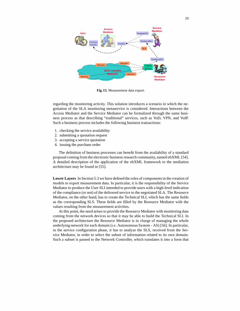
29

ServiceMediator

AccessMediatorUser

ResourceMediator

QoS-capableNetwork

TechnicalSLI

Collected

Measures

TechnicalSLI

TemplateSLI

SLS

UserSLIFormattedUserSLI

Measures

Measures

Measures

Measures

Fig. 13. Measurement data export.

regarding the monitoring activity. This solution introduces a scenario in which the ne-gotiation of the SLA monitoring metaservice is considered. Interactions between theAccess Mediator and the Service Mediator can be formalized through the same busi-ness process as that describing “traditional” services, such as VoD, VPN, and VoIP.Such a business process includes the following business transactions:

1. checking the service availability2. submitting a quotation request3. accepting a service quotation4. issuing the purchase order

The definition of business processes can benefit from the availability of a standardproposal coming from the electronic business research community, named ebXML [54].A detailed description of the application of the ebXML framework to the mediationarchitecture may be found in [55].

Lower Layers In Section 5.3 we have defined the roles of components in the creation ofmodels to export measurement data. In particular, it is the responsibility of the ServiceMediator to produce the User SLI intended to provide users with a high-level indicationof the compliance (or not) of the delivered service to the negotiated SLA. The ResourceMediator, on the other hand, has to create the Technical SLI, which has the same fieldsas the corresponding SLS. These fields are filled by the Resource Mediator with thevalues resulting from the measurement activities.

At this point, the need arises to provide the Resource Mediator with monitoring datacoming from the network devices so that it may be able to build the Technical SLI. Inthe proposed architecture the Resource Mediator is in charge of managing the wholeunderlying network for each domain (i.e. Autonomous System - AS) [56]. In particular,in the service configuration phase, it has to analyze the SLS, received from the Ser-vice Mediator, in order to select the subset of information related to its own domain.Such a subset is passed to the Network Controller, which translates it into a form that

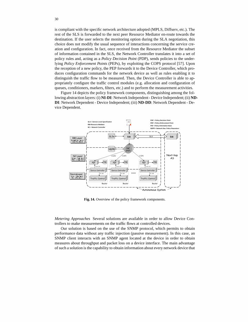
30

is compliant with the specific network architecture adopted (MPLS, Diffserv, etc.). Therest of the SLS is forwarded to the next peer Resource Mediator en-route towards thedestination. If the user selects the monitoring option during the SLA negotiation, thischoice does not modify the usual sequence of interactions concerning the service cre-ation and configuration. In fact, once received from the Resource Mediator the subsetof information contained in the SLS, the Network Controller translates it into a set ofpolicy rules and, acting as a Policy Decision Point (PDP), sends policies to the under-lying Policy Enforcement Points (PEPs), by exploiting the COPS protocol [57]. Uponthe reception of a new policy, the PEP forwards it to the Device Controller, which pro-duces configuration commands for the network device as well as rules enabling it todistinguish the traffic flow to be measured. Then, the Device Controller is able to ap-propriately configure the traffic control modules (e.g. allocation and configuration ofqueues, conditioners, markers, filters, etc.) and to perform the measurement activities.

Figure 14 depicts the policy framework components, distinguishing among the fol-lowing abstraction layers: (i) NI-DI: Network Independent - Device Independent; (ii) ND-DI: Network Dependent - Device Independent; (iii) ND-DD: Network Dependent - De-vice Dependent.

$XWRQRPRXV 6\VWHP

3(33(33(3

'HYLFH� &RQWUROOHUCOPS API



3,%3,%3,%

7UDIILF� &RQWUROTC API



COPS COPS COPS

1&�3'3�

506/6V

1'35

5RXWHU5RXWHU5RXWHU

50

1H[W�KRS$6

SLS

6/6

SLS = Service Level Specification

RM=Resource Mediator

NC = Network Controller

PDP = Policy Decision Point

PEP = Policy Enforcement Point

PIB = Policy Information Base

NDPR = Network Dep. Policy Repository

50� /D\HU��

50� /D\HU��

1&� /D\HU��

1&� /D\HU��

'HYLFH�/D\HU��

'HYLFH�/D\HU��

Fig. 14. Overview of the policy framework components.

Metering Approaches Several solutions are available in order to allow Device Con-trollers to make measurements on the traffic flows at controlled devices.

Our solution is based on the use of the SNMP protocol, which permits to obtainperformance data without any traffic injection (passive measurement). In this case, anSNMP client interacts with an SNMP agent located at the device in order to obtainmeasures about throughput and packet loss on a device interface. The main advantageof such a solution is the capability to obtain information about every network device that

31

supports the SNMP standard protocol. If involved devices are routers or switches madeby Cisco, it is possible to exploit a particular Cisco IOS functionality, named NetFlow.

Exporting Data When the Device Controller, acting as a meter, obtains data about thecontrolled device, it has to forward it to the Resource Mediator. Using this raw data, theResource Mediator can build the Technical SLI.

The Resource Mediator is able to create such an end-to-end document thanks to theinteractions among the involved components, as described below:

1. The Device Controller sends the measurement results to the Policy EnforcementPoint, e.g. using the COPS protocol [58]. This approach perfectly mirrors the policy-based architecture used at service configuration time.

2. Each PEP forwards received data to the Network Controller, which acts as a collec-tor of measurement data from different measurement points;

3. Finally, the Resource Mediator, by gathering information from both its NetworkController and adjacent Resource Mediator, can build the Technical SLI. Such adocument contains information about end-to-end performance metrics related tothe traffic flow specified in the SLS.

5.5 Discussion and Conclusions

In this work, we have presented a component-based architecture for QoS measurementand monitoring. It is clear that the provisioning of such feature is particularly com-plex and critical, since it involves the coordination and orchestrated operation of a largenumber of elements, separately owned and managed along what we have called theprovisioning chain from the service location to the end user. We therefore foresee anumber of issues to be faced: for some of them we believe a solution can be alreadyprovided, while for others the discussion is still wide open. We briefly mention here themain facets of the general issue of QoS monitoring, focusing on the networking infras-tructure. First of all, the collection of monitoring data from the network elements. Thisissue is clearly related to both technical and business aspects. As far as the first ones, thework ongoing in the area of policy based management of network elements is providinga technical framework in which the control and configuration of network nodes will bemuch more straightforward than that currently achievable through the traditional SNMPbased approach. However, it is clear that for global communication infrastructures in-volving large number of nodes with a huge number of active connections we do have aproblem of scalability with respect to the collection and delivery of performance data.In spite of this, we believe that there are features in the existing network architecturesthat might be exploited to reduce at least this problem. For example, in Diffserv basednetwork architectures monitoring of Service Level Agreements can be performed usu-ally per traffic classes and not per single traffic flows, and could be normally limited tothe ingress and egress points of a domain. More detailed performance data collections(in terms of specific flows or network elements) could be triggered only in the presenceof specific demands from the involved parties or in the case of anomalies. As far as thebusiness aspects, i.e. those related to the business nature of the provisioning of com-munication services, we can mention here the one we believe is the most important:

32

trust. In global networks, large scale infrastructures will be managed by a multitude ofdifferent operators, each managing a separate network domain. Quality of Service willtherefore be an issue involving a number of parties, each responsible only for the ser-vice provided in the domain that it directly manages. Such parties will be obliged, at thesame time, to compete and to cooperate with peering entities. Can we foresee a scenariowhere such performance data will be openly (albeit in a controlled way) available? Webelieve that rather than being an obstacle to the deployment of a common frameworkfor SLA monitoring, trust will be an important trigger for it, if not a prerequisite. Infact, we can expect that no operator will start charging for premium services involv-ing infrastructures owned by others without a formal, standardized way for exchangingperformance data about the communication services offered to and received from otheroperators.

A further issue is related to the devising of a common quality of service measure-ment framework. It is clear that performance data should be provided in a way that isindependent of both the network architecture offering the service and the applicationservice demanding it. Our proposal is a first attempt in this direction.

6 Deterministic delay guarantees under the GPS schedulingdiscipline

Under the GPS scheduling discipline traffic is treated as an infinitely divisible fluid. AGPS server that serves N sessions is characterized by N positive real numbers

� � � � � � ��

,referred to as weights. These weights affect the amount of service provided to the ses-sions (or, their bandwidth shares). More specifically, if � � �� denotes the amount ofsession � traffic served in a time interval

�� then the following relation will hold forany session � that is continuously backlogged in the interval

�� ; session � is consid-ered to be backlogged at time � if a positive amount of that session traffic is queued attime � .

� � ��

� � ��

�(3)

The Generalized Processor Sharing (GPS) scheduling discipline has been widelyconsidered to allocate bandwidth resources to multiplexed traffic streams. Its effective-ness and capabilities in guaranteeing a certain level of Quality of Service (QoS) to thesupported streams in both a stochastic ([59–61]) and deterministic ([62–65]) sense havebeen investigated.

In this subchapter the single node case is considered and sessions (sources) areassumed to be

� � � � � leaky bucket constrained and to have a stringent delay require-ment. Such sessions are referred to as QoS sensitive sessions in the sequel; the triplet� � � � � � �� is used in order to characterize the QoS sensitive session � , where � � , � � and� �

represent the burstiness, the long term maximum mean arrival rate and the delayrequirement of session � , respectively.

In the first part of the subchapter the problem of Call Admission Control (CAC) isconsidered. CAC plays a key role in provisioning network resources to meet the QoSrequirements of traffic. It has the function of limiting the amount of traffic accessing

33

the network and can have an important impact on network performance. A CAC algo-rithm is described which fully exploits the bandwidth sharing mechanism of GPS anddetermines the optimal weights

�directly from the QoS requirements of the sessions.

Nevertheless, the use of GPS scheduling discipline can lead to inefficient use of re-sources even if the optimal CAC scheme is employed. In the second part of the subchap-ter a service paradigm is described according to which each session is “represented” bytwo entities – referred to as session components – in the GPS server. Each session’scomponent is assigned a weight and it is served by the GPS server. The work providedby the GPS server to the components of a session is mapped back to the original session.It turns out that the proposed service scheme leads to resource utilization improvement.

Related Work The GPS scheduling discipline has been introduced in [62], [63] wherebounds on the induced delay have been derived for single node and multiple nodessystems, respectively. These (loose) delay bounds have a simple form allowing for thesolution of the inverse problem, that is, the determination of the weight assignmentfor sessions demanding specific delay bounds, which is central to the Call AdmissionControl (CAC) problem.

Tighter delay bounds have been derived in [65] and in [64] (also reported in [66]).These efforts have exploited the dependencies among the sessions -due to the com-plex bandwidth sharing mechanism of the GPS discipline- to derive tighter performancebounds. Such bounds could lead to a more effective CAC and better resource utilization.The inverse problem in these cases, though, is more difficult to solve. For example, theCAC procedure presented in [64] employs an exhaustive search having performancebound calculations as an intermediate step. Specifically, the maximum delay experi-enced by the sessions is determined for a weight assignment and the assignment ismodified trying to maximize an objective function. While the search in [64] terminatesafter a finite number of steps, it does not guarantee that an acceptable assignment doesnot exist if not found.

The fairness oriented nature of GPS scheduling discipline, which follows directlyfrom its definition, makes GPS an appealing choice for a best effort environment, ormore precisely for an environment where fairness is the main concern. Some argumentson why fairness is not necessarily the main concern even in a best effort environmentmay be found in [67] where some state dependent scheduling policies aiming to de-crease loss and / or delay jitter by “sacrificing” fairness are presented.

Modifications / extensions of the GPS scheduling discipline include ([68], [69],[70]). In [68] Service Curve Proportional Sharing (SCPS) has been proposed. It is ageneralization of GPS, according to which the (constant) weighting factors used by theGPS are replaced with well defined varying weights. In [69] a less complex imple-mentation is proposed for the special case of piecewise linear service curves. In [70] amodification of the GPS scheduling discipline, aiming to improve the QoS provided toadaptive sessions is presented, according to which each session is assigned two weights;one weight determines its guaranteed rate and the other weight determines its target rate.

34

6.1 Optimal CAC Algorithm

The optimal CAC algorithm for the GPS scheduling discipline has been derived in [71]by considering a mixed traffic environment in which the bandwidth resource controlledby the GPS server is assumed to be shared by a number of QoS sensitive streams andbest effort traffic. This system will be referred to as a Best Effort Traffic Aware Gener-alized Processor Sharing (BETA-GPS) system.6 The Best Effort Traffic Aware (BETA)GPS system is depicted in figure 15. The BETA-GPS server capacity �� is assumedto be shared by

�QoS sensitive sessions with descriptors

� � � � � � ��

and best effort traffic represented by an additional session. Each session is provided abuffer and the input links are considered to have infinite capacity. Generally, the task

�

Fig. 15. The BETA-GPS system

of CAC is to determine whether the network can accept a new session without causingQoS requirement violations. In the case of a GPS scheduler it should also provide theserver with the weight assignment which will be used in the actual service of the admit-ted calls. A CAC scheme for a GPS server is considered to be optimal if its incapabilityto admit a specific set of sessions implies that no

�assignment exists under which the

server could serve this set of sessions (respecting all QoS requirements).An optimal CAC scheme for the BETA-GPS system should seek to maximize the

amount of service provided to the (traffic unlimited) best effort session under any arrivalscenario and over any time horizon, while satisfying the QoS requirement of the (trafficlimited) QoS sensitive sessions. That is, it should seek to maximize the normalized7

weight assigned to the best effort traffic (�� ), while satisfying the QoS requirement of

QoS sensitive sessions. Obviously, maximizing the weight assigned to the best efforttraffic is equivalent to minimizing the sum of weights assigned to the QoS sensitivesessions.

Optimal CAC Scheme for the BETA-GPS system In the sequel only the rationaleof the optimal CAC algorithm is described and a numerical example is provided; thedetailed algorithm may be found in [71].

The CAC problem for a GPS system is simplified in view of the following Theorem(Theorem 3, [62]): If the input link speed of any session � exceeds the GPS service

6 In a system where only QoS sensitive sessions are present the existence of an extra sessionmay be assumed and the presented algorithm be applied (see [71]).

7 Without loss of generality, it is assumed that��

35

rate, then for every session � , the maximum delay �� and the maximum backlog� ��

are achieved (not necessarily at the same time) when every session is greedy starting attime zero, the beginning of a system busy period. It is noted that a GPS system busyperiod is defined to be a maximal time interval during which at least one session isbacklogged at any time instant in the interval. A session � is characterized as greedystarting at time

�if it sends the maximum allowable amount of traffic starting at time�

and an all-greedy GPS system is defined as a system in which all the sessions aregreedy starting at time 0, the beginning of a system busy period.

The aforementioned theorem implies that if the server can guarantee an upper boundon a session’ s delay under the all greedy system assumption this bound would be validunder any (leaky bucket constrained) arrival pattern. Thus, in the framework of the CACproblem it is sufficient to examine only all greedy systems.

It [71] it has been shown that a given acceptable�

assignment is converted to theoptimal one if each QoS sensitive session’s busy period is expanded as much as its QoSwould permit, starting from the set of QoS sensitive sessions that empty their backlogfirst in order.8 This implies that in order to determine the optimal

�assignment it is

sufficient to allocate to the QoS sensitive sessions such weights that their QoS wouldbe violated if their busy periods were expanded.

In order to determine these optimal weights the CAC algorithm of [71] emulates theall greedy system and examines the QoS sensitive sessions at all time instants coincidingwith either the delay bound or the backlog clearing time of some session; these timeinstants are referred to as checkpoints in [71]. For each QoS session the algorithmcomputes two quantities (two potential weights); the minimum weight that is necessaryfor the QoS requirements of the session to be met up to the specific time instant andthe weight that is necessary for the QoS requirements of the session to be met after thespecific time instant, denoted as

�� and� �� at the checkpoint

� ,respectively.If

�� session � is assigned a weight� � �� , since this is the

minimum weight that could be assigned; else the specific session is examined againat the next checkpoint. In order to apply the aforementioned procedure the algorithmkeeps track of the bandwidth that is available to the still backlogged sessions (a greedy( � � � � � ) constrained session requires a rate equal to

� �after it empties its backlog, and

thus, the additional (compared to� �

) bandwidth that the session utilizes until it emptiesits backlog is shared among the still backlogged sessions in proportion to their weight).

Next a numerical example is provided, where the optimal CAC scheme for theBETA-GPS system is compared with the effective bandwidth-based CAC scheme. De-terministic effective bandwidth ([72]) can be used in a straightforward way to give asimple and elegant CAC scheme for the GPS scheduler. A similar approach is followedin [61] for the deterministic part of their analysis. The deterministic effective bandwidthof a

� � � � � � �� session is given by � �� . It is easy to see that the re-

quirements of the QoS sensitive sessions are satisfied if they are assigned weights such

that� � � � ��

( � �� !�� !��

�#" �� %$ �'&�().

8 A � assignment is characterized as acceptable if it is feasible (that is�� ) � )and delivers

the required QoS to each of the supported QoS sensitive sessions; a � assignment is character-ized as more efficient than another if the sum of � ’s

�� under the former assignment issmaller than that under the latter.

36

Two traffic mixes are considered which are denoted as Case 1and Case 2 in Table 1where the parameters of the sessions for each case are provided. All quantities are con-sidered normalized with respect to the link capacity C. In order to compare the optimal

Table 1. Sessions under investigation

Case 1 � �� Case 2 � �� 0.04 0.16 0.04 0.64� � 0.01 0.01 0.04 0.01� � 1 4 4 16� �� 0.04 0.04 0.04 0.04

CAC algorithm with the effective bandwidth-based CAC scheme the following scenariois considered. The effective bandwidth-based CAC scheme admits the maximum num-ber of sessions under the constraint that a nonzero weight remains to be assigned tobest effort traffic. From Table 1 it can be seen that the effective bandwidth of each QoSsensitive session is 1/25 of the server’s capacity (which is considered to be equal to thelink capacity ( � � � )), implying that for the BETA-GPS system at most 24 QoSsensitive sessions can be admitted under the effective bandwidth-based CAC scheme.This means that

� �� must hold and that the best effort traffic is as-signed weight equal to 0.04 for each such triplet (

� �,� � and

�� denote the number of

admitted sessions of type� �

,� � and

�� respectively).

For each triplet� � � � � � � �� , � �� , the weight assigned to the

best effort traffic by the optimal CAC scheme is computed. The results are illustrated infigure 16.

�

Case 1�

Case 2

Fig. 16. Weight assigned to the best effort traffic according to the (1) optimal CAC (2) effectivebandwidth-based CAC scheme, both under the constraint � � � � � � � �� . The minimumguaranteed rate to the best effort traffic is � ��

37

Decomposition module

Service module module

Service mapping

session’s j traffic

session’s i traffic

traffic replicasession’s k

LT component

traffic replica

GPSCG

LT componentsession’s i

traffic replica

real buffers

session’s j

B component

B component

Real System

best effort traffic

session’s k traffic

traffic replicabest effort

Virtual System

PSfrag replacements

� � � � � � � � � ��

� � � � � � � � �

� � � � � � � � � � � ��

� � � � ��

� � � � � � � � � � � � �

� � � �

� � � �

� � � � � � � � � ��

� � � � ��

� � �

� � � � � � � � � � � � �

� � � �

� � � �

� � � � � � � ��

� � � �

� � � �

� � � � �

� � � � �

Fig. 17. The DS-system

6.2 Decomposition-based Service (DS-) Scheme

According to the Decomposition-based Service (DS-) scheme, which is depicted in fig-ure 17, sessions are not served directly by the GPS scheduler. The GPS scheduler isemployed by a Virtual System which is provided with an exact replica of each session’straffic. In the Virtual System some of the sessions (replicas) are decomposed into twocomponents, by engaging properly dimensioned leaky buckets, one for each session.These two components are buffered in separate virtual buffers and are assigned weightsin proportion to which they are served by the GPS scheduler. The real traffic of a ses-sion is served at any time instant at a rate equal to the sum of the service rates of itscomponents in the Virtual System.

The Virtual System is necessary (that is, the decomposition can not be applied di-rectly on the original sessions) so that the real traffic of each session remains in a com-mon buffer in order to avoid “packet reordering”; that is, to ensure that each session’straffic leaves the system in the order it arrived. The Virtual System may be consideredto consist of three modules (see figure 17): (a) the decomposition module responsiblefor the decomposition of the replicas of the sessions (b) the service module responsiblefor determining the service provided to each session’s components, and (c) the servicemapping module which maps the service provided to the sessions components back tothe original sessions.

Each session �� may be considered as the superposition (aggregation)of two component sessions �� and �� , � � � � � � � �

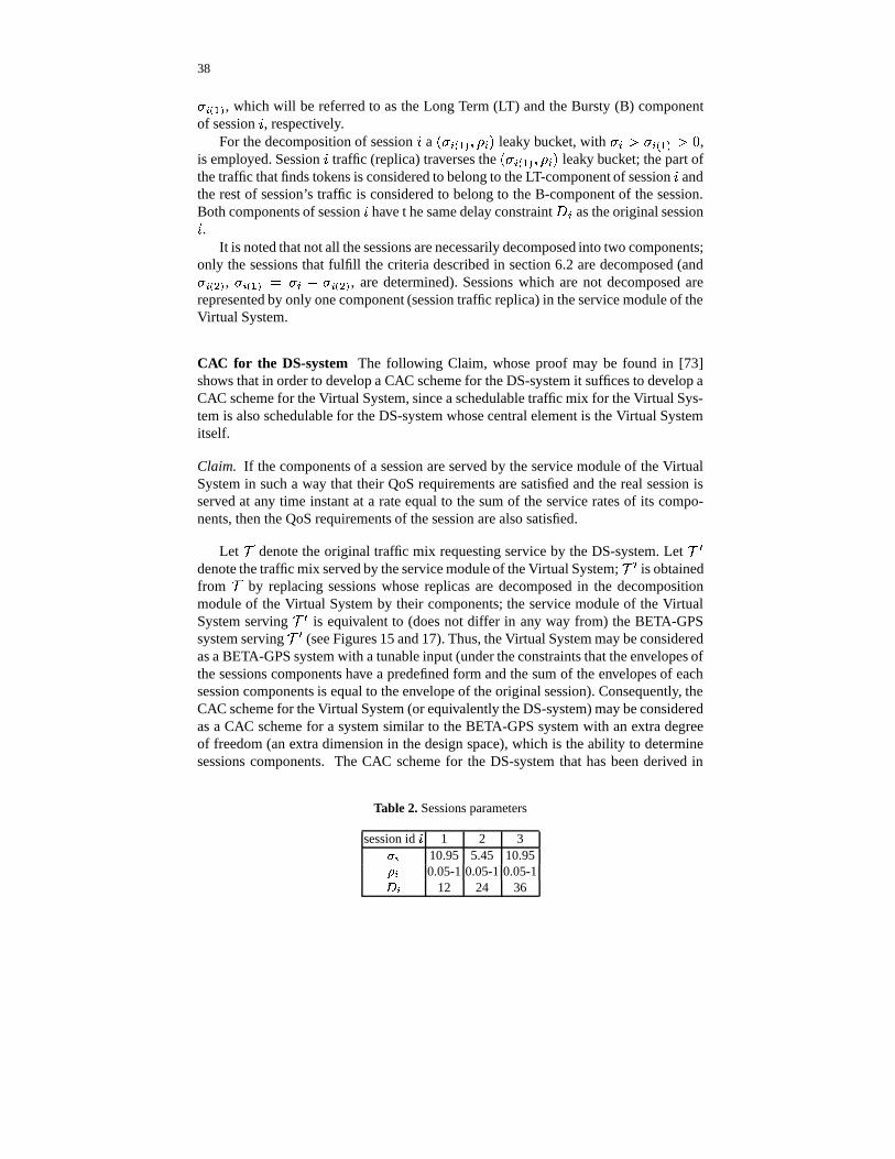
38

� � � � � , which will be referred to as the Long Term (LT) and the Bursty (B) componentof session � , respectively.

For the decomposition of session � a� � � � �� leaky bucket, with � � � � � � �� ,

is employed. Session � traffic (replica) traverses the� � � � �� leaky bucket; the part of

the traffic that finds tokens is considered to belong to the LT-component of session � andthe rest of session’s traffic is considered to belong to the B-component of the session.Both components of session � have t he same delay constraint � �

as the original session� .

It is noted that not all the sessions are necessarily decomposed into two components;only the sessions that fulfill the criteria described in section 6.2 are decomposed (and� � � � � , � � � �� , are determined). Sessions which are not decomposed arerepresented by only one component (session traffic replica) in the service module of theVirtual System.

CAC for the DS-system The following Claim, whose proof may be found in [73]shows that in order to develop a CAC scheme for the DS-system it suffices to develop aCAC scheme for the Virtual System, since a schedulable traffic mix for the Virtual Sys-tem is also schedulable for the DS-system whose central element is the Virtual Systemitself.

Claim. If the components of a session are served by the service module of the VirtualSystem in such a way that their QoS requirements are satisfied and the real session isserved at any time instant at a rate equal to the sum of the service rates of its compo-nents, then the QoS requirements of the session are also satisfied.

Let � denote the original traffic mix requesting service by the DS-system. Let ��denote the traffic mix served by the service module of the Virtual System; �� is obtainedfrom � by replacing sessions whose replicas are decomposed in the decompositionmodule of the Virtual System by their components; the service module of the VirtualSystem serving �� is equivalent to (does not differ in any way from) the BETA-GPSsystem serving �� (see Figures 15 and 17). Thus, the Virtual System may be consideredas a BETA-GPS system with a tunable input (under the constraints that the envelopes ofthe sessions components have a predefined form and the sum of the envelopes of eachsession components is equal to the envelope of the original session). Consequently, theCAC scheme for the Virtual System (or equivalently the DS-system) may be consideredas a CAC scheme for a system similar to the BETA-GPS system with an extra degreeof freedom (an extra dimension in the design space), which is the ability to determinesessions components. The CAC scheme for the DS-system that has been derived in

Table 2. Sessions parameters

session id � 1 2 3� � 10.95 5.45 10.95� � 0.05-1 0.05-1 0.05-1� � 12 24 36

39

10−1

100

10−1

100

10−1

100

ρ1

ρ2

ρ3

PSfrag replacements

Fig. 18. BETA-GPS system employing the op-timal CAC scheme for the BETA-GPS

10−1

100

10−1

100

10−1

100

ρ1

ρ2

ρ3

PSfrag replacements

Fig. 19. DS-system employing the D CACscheme

[73] and is referred to as the D CAC scheme (Decomposition-based Call AdmissionControl scheme) is a generalization of the optimal CAC scheme for the BETA-GPS, inthe same way as the DS-system is a generalization of the BETA-GPS system. It may beconsidered as consisting of two distinct functions: (a) one responsible for determiningwhich sessions of the original traffic mix will be decomposed in the Virtual System andthe exact form of their components, and (b) one responsible for determining the weightassignment for the sessions components. The optimal CAC scheme for the BETA-GPSis employed for the determination of the weight assignment of the session components.The other function, which is responsible for determining the session components issuch that a session replica is decomposed in the Virtual System only if (and in such away that) this decomposition: (a) leads to better (or at least not worse) resource utiliza-tion, and (b) the session is assigned a total weight (sum of the weights of the sessioncomponents) no greater than if it were not decomposed.

These conditions imply that the decomposition procedure is such that it leads to atraffic mix �� – starting from a traffic mix � – for which the optimal CAC schemefor the BETA-GPS returns total weights for the components of any session that aretypically smaller and never larger than those identified by applying the optimal CACscheme for the BETA-GPS to the original traffic mix � . This allows a typically greaterand never smaller weight to be assigned to the best effort traffic, for the traffic mixes thatare schedulable in the BETA-GPS system. In addition, some traffic mixes that are notschedulable by the GPS in the BETA-GPS system, can be admitted in the DS-system(whose service module is a GPS server), and thus, the transformation of � to � � maybe considered to lead to an indirect expansion of the schedulability region of GPS.

The details of the D CAC scheme may be found in [73]. In the sequel a numericalexample is provided that demonstrates the improvement in resource utilization that canbe achieved by employing the DS-system. The considered traffic mix consists of threesessions whose parameters are shown in Table 2. �� and �� are kept constant while� � takes values between 0.05 and 1 (the step is equal to 0.02). The link capacity isassumed to be equal to 1. In figure 18 the maximum long term rate of session 3 ( � ),such that the traffic mix is schedulable, is depicted as a function of �� and � � for theBETA-GPS system employing the optimal CAC scheme for the BETA-GPS . In figure19 the corresponding plot is given for the case of the DS-system employing the D CACscheme.

40

7 MPEG Traffic Modeling at the Frame and GoP Levels UsingGBAR and D-BMAP Processes

7.1 Introduction

Modern broadband telecommunications networks are intended to deliver traffic gener-ated by multimedia applications. Video-on-Demand (VoD) is an example of such ap-plications. Traffic generated by VoD servers must be delivered to destinations usinga certain network technology. To provide an adequate quality of service (QoS), somequality control mechanisms have to be implemented in the network.

It is well known that uncompressed video information can easily throttle the avail-able bandwidth. In order to achieve efficient transmission of such traffic, video infor-mation must be compressed and encoded in accordance with one of the existing com-pression algorithms. Today, one of the most used algorithms is MPEG.

Modeling of variable bit rate (VBR) videotraffic has become an important issuesince it provides the starting point for both theoretical analysis and engineering design.The source models of different types of videotraffic are needed to design and study thenetwork performance and also to predict the QoS that a particular video applicationmay experience at different levels of network congestion [74, 75].

A number of video source models have been proposed in literature. Recently, mostattention has been paid to MPEG traffic modeling using discrete- and continuous-timeMarkov chains [76, 75]. Such models produce an excellent approximation of both thehistogram of frame sizes and the autocorrelation function (ACF) of the empirical databut they are computationally inefficient because the construction of these Markov mod-ulated processes from empirical data involves the so-called inverse eigenvalue problem[76, 75]. This drawback restricts their use in simulation studies where it is necessary toproduce the model ”on the fly”.

Firstly, we propose a novel frame level two-step MPEG modeling algorithm thatemulates the behavior of a single MPEG-1 elementary video stream. The proposedalgorithm captures well the distribution of frame sizes and the ACF at frame level.

Then, based on the special case of the D-BMAP process, we model the smoothedtraffic from the single MPEG source. Based on the statistical analysis of MPEG trafficat the group of pictures (GoP) level we propose to limit the state space of the modulat-ing Markov chain of the D-BMAP process such that it now employs only four states.The limited state space allows us to decrease the complexity of the algorithm while thenecessary accuracy is retained. Our D-BMAP model is simple enough, captures boththe histogram of relative frequencies and the ACF of a single smoothed MPEG traf-fic source, allows an analytical evaluation of the queuing systems and can be used insimulation studies.

It should be noted that in modeling MPEG traffic we focus on MPEG data, ignoringauxiliary information: the sequence header, packet headers etc.

The rest of the section is organized as follows. In the next subsection we brieflyoutline MPEG traffic. Then we consider our modeling methodology. In Section 7.3we present a GBAR(1) MPEG traffic model. Section 7.4 provides an MPEG trafficmethodology based on the D-BMAP process. Conclusions are drawn in the last section.

41

7.2 MPEG Traffic

MPEG traffic is characterized by high peak rates and drastic short-term rate changes.These features cause losses within node buffers or remarking within traffic conditioners.To deal with these problems to some extent we assume that MPEG traffic is smoothedat the group of pictures (GoP) level as follows:

��

� ��

� � � � � � � � � !��

� � (4)

where N is the number of frames, � � !�� is the length of the GoP, X(n) denotes the sizesof individual frames and

� � �� denotes the sizes of the smoothed sequence. In ourstudy GoP has (12,3,2) structure [77] and we can only use those smoothing patternswhose length is divisible by 12. We set m=12.

The outlined approach does not require any computational resources during thetransmission of video, provides a deterministic delay and efficiently employs the framestructure of MPEG traffic. This approach can thus be used in VoD systems.

7.3 VoD Traffic Models

The GBAR(1) modeling algorithm has a two-step structure. Heyman in [78] shows thatthe model of MPEG traffic at frame level must incorporate three strongly auto- andcross-correlated processes. These are I-frame process, P-frame process and B-frameprocess. Therefore, we should take into account the correlation structure of empiricaldata. At the first step of the proposed algorithm we use the property that I-frames arecoded autonomously without reference to preceding or following frames, and, thereforewe can state that the sizes of I-frames are independent of the sizes of P- and B-frames.Based on this we propose to model the I-frame generation process as an independentstochastic process. In order to accomplish this we use the GBAR(1) process. The se-quence of sizes of I-frames that is obtained during the first step is used together withintra-GoP correlation information as initial data for the second step of the algorithm.

Before discussing the details of the algorithm we point out the necessary prerequi-sites. As has been shown in [79] the distribution of intra-frame sizes at the output ofan H.261 codec can be approximated by a negative-binomial distribution and its con-tinuous equivalent - the gamma distribution. The intra-frame coding scheme utilized byH.261 codecs is almost identical to that used for I-frame coding in the MPEG standard.Therefore, we can expect that the gamma distribution will provide a good approxima-tion for the I-frame sizes. To prove this we compared an empirical I-frame size distri-bution and the gamma distribution for the pattern “Star Wars” by the quantile-quantilestatistical analysis. We used the following parameter values: shape parameter was set to3.0 and scale parameter was set to 2.6E-5. These parameters were derived directly fromthe empirical distribution. We have noticed in [80] that such an approach gives a goodapproximation for the empirical data.

The property that allows us to proceed from the I-frame generation process to anMPEG aggregate frame generation process is a strong dependence between I-framesizes and B- and P-frame sizes within the same GoP. This property was discovered by

42

Lombardo et al. [81, 82], clearly explained in [76] and later were called ”intra-GoPcorrelation”.

I-frame Process In order to represent the I-frame generation process we propose to usethe GBAR(1) process. It was originally presented by Heyman [78], where it was usedas the approximation model for the frame size distribution of H.261 codec. The maindistinctive feature of the process appears in the geometrical distribution of its ACF.This property allows us to model the ACF of the empirical data that exhibits some sortof short range dependence (SRD) behavior. Moreover, the marginal distribution of theframe size sequence is a gamma distribution.

Let � �� be a random variable with a gamma distribution with shape parameter�and scale parameter � , and let � � � �� be a random variable with a beta distribution

with parameters � and � . The GBAR(1) process is based on two well-known results: thesum of independent random variables � �� and � �� is a � �� randomvariable, and the product of independent random variables � �� and � �� isa � �� random variable.

Thus, if we denote � �� , � � �� and � � �� and

if they are mutually independent, then � � � � �� is a stationary stochastic

process � � � � � � � � � � ��

with marginal distribution � �� . The ACF is geometricaland given by �� . Parameters

�and � can be directly estimated from empirical

data. Assume that the ACF is above zero for sufficiently large lag k: �� then thefollowing equation holds

� � � and�

is obtained.Random variables with gamma or beta distributions generate non-integer values

because they are continuous. Since the number of bits in the frame is a discrete randomvariable we round the values obtained from this process to the nearest integer.

Approximation of Intra-GoP Correlation In order to approximate the intra-GoP cor-relation structure and to obtain sizes of P- and B-frames, the algorithm proposed in[76] can be used. The algorithm is intended to clarify the dependency between themean value and the standard deviation of I-frames and the sizes of appropriate P- orB-frames. These dependencies are determined as follows:

� � �� $ �� (5)

where� � is the mean value of the appropriate frame (P or B), � � is the standard

deviation of the P- or B-frames, and� �

is the size of the I-frame. Results are shownin [76, 80–82] where it was shown that these dependencies can be approximated bystraight lines.

The mean value and the standard deviation given by (5) serve as initial parame-ters for certain probability distributions. These probability distributions will allow usto obtain B- and P-frame sizes holding the I-frame size constant (or, more precisely,an interval of I-frame sizes). Note that in this case, the output values will vary evenfor constant I-frame size. This property of the model emulates the behavior of the realcodecs.

43

Approximation of B- and P- frame sizes It has been shown that histograms of theB- and P-frame sizes corresponding to a certain I-frame size can be approximated bya gamma distribution [81, 82]. The ACF of the P- and B-frame generation processesholding the I-frame size constant have the SRD property only. Since the GBAR processcaptures well all of the properties mentioned here we use this process as a model for P-and B-frame generation processes [80].

7.4 Traffic Modeling at the GoP Level

To model the smoothed traffic at the GoP level from the single MPEG source we pro-pose to use the D-BMAP process. In each state of the modulating Markov chain of thisprocess we can use an arbitrary distribution and the ACF of the process can be made toconstitute a good approximation of the empirical ACF.

Consider general characteristics of the D-BMAP process. Let � � ��

be the D-BMAP arrival process. In accordance with D-BMAP, the number of arrivingpackets in each interval is modulated by an irreducible aperiodic discrete-time Markovchain (DTMC) with M states. Let D be the transition matrix of this process. Assumethat the stationary distribution of the modulating DTMC is given by the vector

�� . We

define the D-BMAP process as a sequence of matrices � � �� , each ofwhich contains probabilities of transition from state to state with � �� arrivalsrespectively [83]. Note that the number of arrivals in real models is always bounded.

Let the vector�� be the mean rate vector of the D-BMAP

process. The input rate process of the D-BMAP � � � � � ��

is defined by��

�with � � � � � � while the Markov chain is in the state i at the

time slot n [80]. The ACF of the rate process is given by [83]:

� � � � � ��

� ��

�� (6)

where � � is the ��

eigenvalue of � ,�� and

�� are the eigenvectors of D and��

is avector of ones.

Note that the ACF of the rate process consists of several geometric terms. Such be-havior produces a good approximation of empirical ACFs that exhibit near geometricalsum decays [76, 84]. The number of geometrical terms composing the ACF dependson the number of eigenvalues which, in turn, depends on the number of states of theDTMC [85]. Thus, by varying the number of states of the modulating Markov chain wecan vary the number of geometrical terms composing the ACF.

ACF Approximation In order to approximate the empirical ACF of MPEG traffic atthe GoP level from the single MPEG source we use the method originally proposed in[76]. Particularly, we minimize the error of ACF approximation � by varying the values

44

of coefficients� � � � � � ��

�for each

� � � � � � � � in accordance with:

� � ��

� �� (7)

where i is the lag, �� is the lag when the empirical ACF reaches the confidential interval,and � � �� is the value of the ACF for lag i.

We note that we do not consider here those cases when� �� . This is because

with the increasing of the number of coefficients, which approximate the empiricalACF, the number of eigenvalues also increases and, therefore, the state space of themodulating Markov chain expands significantly. Thus, it is wise to keep the state spaceas small as possible and, from this point of view,

� � presents the best trade-offbetween the accuracy of the approximation of the empirical ACF and the simplicity ofthe modulating Markov chain. Note that with

� � the number of states of modulatingMarkov chain of the D-BMAP process may not exceed three.

At this stage the only approximation error is induced. This is the error of ACFapproximation � � � � by two geometrically distributed terms.

Approximation by the Input Rate Process The construction of Markov modulatedprocesses from empirical data involves a so-called inverse eigenvalue problem. It isknown that the general solution of this problem does not exist. However, it is possibleto solve such problems when some limitations on the form of the eigenvalues are set[76, 75].

Our limitation is that the eigenvalues should be located in the� � � � � fraction of the

X axis. Note that one part of limitation� � � � � �#" � is already fulfilled since all

eigenvalues of the one-step transition matrix of an irreducible aperiodic Markov chainare located in the

� � � � � fraction of X axis [85]. The second part �� #" � shouldbe fulfilled by the solution of the inverse eigenvalue problem.

We propose to construct the D-BMAP arrival process from two simple D-BMAPprocesses with a two-state modulating Markov chain. Let � � � � � ��

�be the

D-BMAP arrival process, which models the smoothed traffic from an MPEG source,and � � � ��

�be the empirical process of GoP sizes. � ��

��

�and � ��

� � � � ��

are two simple two-state D-BMAP processes(switched D-BMAP, SD-BMAP).

It is known that the rate process of simple an SD-BMAP can be statistically char-acterized by the triplet

� � � � � � � � [86], where� � � is the mean arrival rate of the

process, is the variance of the D-BMAP process and � is the real eigenvalue of themodulating Markov chain which is not zero [85]. However, in order to define the rateprocess of the SD-BMAP, we should provide four parameters

� � � �� , where � �

and � � are the mean arrival rates in state 1 and state 2 respectively,�

is the probabilityof transition from state 1 to state 2 and

�is the probability of transition from state 2 to

state 1.If we choose � �

as the free variable [76] with constraint � � � � �� to satisfy

�� [86], we can obtain the other variables from the following equations [76,

45

86]:

� � � � � � � ��

� ��

� �� (8)

Therefore, if we set � ��

� � , � �� ,

� � � � ��

�� , and

choose � ��

and � ��

�such that �

��

�� and � �

��

�� we get both SD-

BMAP arrival processes whose superposition gives us the D-BMAP process with thesame ACF and mean arrival rate as the empirical data. The one-step transition matrixof the superposed process is given by the Kronecker product of composing processes� �

�� .

It is clear from (8) that there is a degree of freedom when we choose the parameters�

��

and � ��

�. Moreover, the additional degree of freedom arises when we choose the

values of� ��

�� and

� �� . Thus, there is an infinite number of D-BMAP arrival

processes with the same mean arrival rate� � � �� which approximate the empirical

ACF with error � .We also note that from the definition of the Kronecker product it follows that the

eigenvalues of the matrix D which is the Kronecker product of matrices ��

and � ��

with respective eigenvalues � �� , and � �

�� , has eigenvalues

which are given by � � � ��

�� . Therefore, there is an additional

error in the empirical ACF approximation, which is caused by only one eigenvalue� ��

�� of the superposed process, since the one-step transition matrix of a two-state ir-

reducible aperiodic Markov chain possesses two eigenvalues and one of them is always1. Therefore, the error of the ACF approximation can be expressed precisely:

� � � ��

� ��

�� (9)

where � � ��

��

.

Approximation of Relative Frequencies of GoP sizes Note that the above mentionedderivation of the D-BMAP process restricts us to the mean arrival rate and the ACFand does not take into account the histogram of relative frequencies of GoP sizes. Tohave assurance that both the histogram and ACF are matched we should assign the PDFof GoP sizes to each state of the 4-state modulating DTMC such that the whole PDFmatches the histogram of GoP sizes.

Assume that the histogram of relative frequencies has m bins. Therefore, each PDFin each state of the modulating Markov chain should have not less than m bins. Sincethe stationary probabilities of the modulating Markov chain of the D-BMAP processare known for each PDF the following set of equations should hold:��

� ��

��

� ��

��

� �� (10)

where � � � � � � � � � � � �� is the number of histogram bins, � � �� and�� are the relative frequency and probability respectively corresponding to the

� �

46

bin in the ��

state of the modulating Markov chain, ��

is the mean arrival rate in statei and

�is the length of histogram intervals.

Note that we have only� � � � � � � equations while there are � � unknowns. We also

should note that in general, if the Markov chain has M states and there are � histogrambins the number of unknowns is

� � and we have only � � � � equations. It is seen thatwith the increasing the number of states of the modulating Markov chain the complexityof the task increases rapidly. This is the additional reason why we should keep the statespace of the modulating Markov chain as small as possible.

In order to get values of �� we propose to use the

random search algorithm. In accordance with this algorithm we should firstly choosethe necessary error of the approximation of histogram of relative frequencies � andthen assign the PDF to each state of the 4-state modulating Markov chain to yield (10).Note that the time the algorithm takes to find the suitable solution depends on the error

� .

7.5 Modeling Results

We have applied both algorithms [80, 84] to all traces from the MPEG trace archive[77] and found that it matches both the histogram of relative frequencies of GoP sizesand empirical ACF fairly well. In order to compare the model with empirical data wegenerated exactly the same amount of I-, P-, B- and GoP sizes as the empirical traces.Here we present a discussion of comparison studies between both models and “StarWars” trace given in [80, 84].

In order to compare the distribution function of the models with corresponding his-tograms of relative frequencies (I-, P- and B-frame sizes for frame level and GoP sizesfor GoP level) we have performed a chi-square statistical test. The test has shown thatthe statistical data of GoP sizes belong to the PDF of the D-BMAP model given a levelof significance of 0,05 and statistical data of I-, P- and B-frame sizes belong to corre-sponding distribution functions of the GBAR(1) model given a level of significance of0,1.

Considering the ACF behavior we note that up to lag 50-100 the empirical ACFand the ACF of the GBAR model are close to each other. Later, the ACF of the modelquickly decays to zero. With the increasing of p parameter the correlation has a strongtrend to rise for all lags. Thus, the model overestimates the ACF up to lag 80 and,consequently, is not able to give a good approximation for larger lags. At the frame levelthe D-BMAP model approximates the behavior of the empirical ACF of GoP sizes wellfor any lag.

One of the major shortcomings of the GBAR(1) model stems from the fact that thereal data trace contains several frames with a very high number of bytes. The modelcan approximate this property in case of small values of p parameter, which will lead tounderestimation of the ACF for large lags. There is a trade-off between two propertiesof the model: the distribution of frame sizes and the ACF. One possible solution is thecareful choice of p values.

47

7.6 Conclusions

In this section we have considered the modeling of an MPEG-1 video elementary streamat the output of the codec. We propose two MPEG traffic models aimed at differentMPEG logical levels: frame and group of pictures (GoP) levels.

On the frame level we proposed an extension of a modeling methodology proposedin [78] and [76]. We have used a two-step approach in order to model the video framessequence. At the first step we approximate the I-frames generation process by a GBARprocess. The second step consists of the approximation of frame sizes based on both theoutput of the GBAR process and intra-GoP correlations. The proposed algorithm pro-vides a simple model of the MPEG source based on three cross-correlated processes.The algorithm captures well both the distribution of frame sizes and the ACF of empiri-cal data. The GBAR model is fast, computationally efficient and captures well the SRDbehavior of the ACF and the distribution of frame sizes. It can be used in simulationstudies where there is a need to generate MPEG traffic “on the fly“.

The GBAR process needs only a few parameters, which can be estimated directlyfrom the analysis of empirical data. This is a big advantage of the GBAR source modelcompared to other models of video traffic sources.

Our model at the GoP level is a refinement of the model originally proposed in [76].The model of smoothed MPEG traffic at the GoP level from a single MPEG source isbased on a special type of D-BMAP process. Based on the statistical analysis of MPEGtraffic at the GoP level we limited the state space of the modulating Markov chain of theD-BMAP process. The limited state space allows us to decrease the complexity of thealgorithm while the necessary accuracy of the approximation is retained. The D-BMAPmodel captures both the histogram of relative frequencies and the empirical ACF of asingle smoothed MPEG traffic source. In addition, it is simple enough and can easily beused in simulation studies even when it is necessary to generate the model “on the fly“.The model is useful for both analytical evaluation of queuing systems and simulationstudies.

8 An Open Architecture for Diffserv-enabled MPLS networks

8.1 Introduction

The Internet has quickly evolved into a very critical communications infrastructure,supporting significant economic, educational and social activities. Simultaneously, thedelivery of Internet communication services has become very competitive and end-usersare demanding very high quality services from their service providers. Consequently,performance optimization of large scale IP networks, especially public Internet back-bones, has become an important problem. This problem is addressed by traffic engi-neering, which encompasses the application of technology and scientific principles tothe measurement, characterization, modeling and control of Internet traffic. Enhancingthe performance of an operational network, at both the traffic and resource levels, aremajor objectives of Internet traffic engineering; this is accomplished by addressing traf-fic oriented performance requirements, while utilizing network resources economicallyand reliably. Traffic engineering deals essentially with the selection of optimal paths

48

that different flows should follow in order to optimize resource utilization and satisfyeach flow’s requirements. Historically, effective traffic engineering has been difficult toachieve in public IP networks, due to the limitations of legacy IGPs, which are adapta-tions of shortest path algorithms where costs are based on link metrics. This can easilylead to unfavorable scenarios in which some links become congested while others re-main lightly loaded [87].

The development and introduction of Multi-Protocol Label Switching (MPLS) [88]has opened new possibilities to address some of the limitations of IP systems concerningtraffic engineering. Although MPLS is a relatively simple technology (based on theclassical label swapping paradigm), it enables the introduction of traffic engineeringfunction in IP networks because of its support of explicit LSPs, which allow constraint-based routing (CBR) to be implemented efficiently. For this reason, MPLS currentlyappears as the best choice to implement traffic engineering in IP networks [89].

It is clear, however, that in modern IP networks, the need for supporting flows withdifferent QoS requirements would demand additional mechanisms, such as those thatperform policing on the incoming traffic, classify packets in different service classesand assure them the required quality of service. The introduction of appropriate packetscheduling disciplines and of architectures for differentiating services, such as Diffserv[90], can be used for this purpose. When MPLS is combined with Diffserv and ex-plicit routing, we have a powerful architecture which allows both traffic engineeringand quality of service provisioning. The interoperability between MPLS and Diffservhas already been the subject of studies from the Internet community and the resultingarchitecture is defined in RFC 3270 [91].

Believing in the benefits of a Diffserv-enabled MPLS architecture, this paper presentsan experimental approach to the study of the interoperability between the Diffserv andMPLS paradigms. Few implementations currently exist of both architectures and mostof them represent proprietary solutions, with device-specific contaminations. With re-spect to Diffserv, two different open source implementations have been considered,based respectively on the FreeBSD and Linux operating systems. The former is theALTQ [92] package developed at the Sony Research Laboratories in Japan; the latteris the Traffic Control (TC) [93][94] module. Such modules basically make the funda-mental traffic control components available, which are needed in order to realize theDiffserv paradigm: classifiers, schedulers, conditioners, markers, shapers, etc. As faras MPLS, a brand new package running under Linux has been utilized [95]. In orderto gain experience with this platform and to evaluate the performance overhead due topushing/popping the MPLS label some measurements have been performed, shown inSect. 2.

The testbed set up at the University of Naples makes use of the Linux implementa-tions of both Diffserv and MPLS to analyze four different scenarios (best effort, Diff-serv, MPLS and Diffserv over MPLS), in order to appreciate the efficiency of Diffserv intraffic differentiation and to evaluate the interoperability between MPLS and Diffserv.Section 3 describes the experimental testbed, while Sect. 4 shows the results obtainedfrom experimentations and draws a comparison among the four different scenarios.

We point out that the trials described in this paper are carried out by statically con-figuring each router, while a dynamic configuration is required to serve each incoming

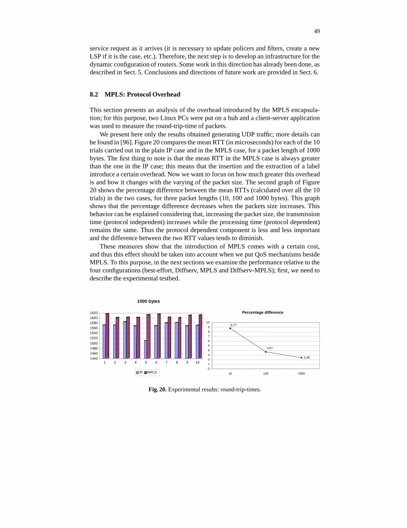
49

service request as it arrives (it is necessary to update policers and filters, create a newLSP if it is the case, etc.). Therefore, the next step is to develop an infrastructure for thedynamic configuration of routers. Some work in this direction has already been done, asdescribed in Sect. 5. Conclusions and directions of future work are provided in Sect. 6.

8.2 MPLS: Protocol Overhead

This section presents an analysis of the overhead introduced by the MPLS encapsula-tion; for this purpose, two Linux PCs were put on a hub and a client-server applicationwas used to measure the round-trip-time of packets.

We present here only the results obtained generating UDP traffic; more details canbe found in [96]. Figure 20 compares the mean RTT (in microseconds) for each of the 10trials carried out in the plain IP case and in the MPLS case, for a packet length of 1000bytes. The first thing to note is that the mean RTT in the MPLS case is always greaterthan the one in the IP case; this means that the insertion and the extraction of a labelintroduce a certain overhead. Now we want to focus on how much greater this overheadis and how it changes with the varying of the packet size. The second graph of Figure20 shows the percentage difference between the mean RTTs (calculated over all the 10trials) in the two cases, for three packet lengths (10, 100 and 1000 bytes). This graphshows that the percentage difference decreases when the packets size increases. Thisbehavior can be explained considering that, increasing the packet size, the transmissiontime (protocol independent) increases while the processing time (protocol dependent)remains the same. Thus the protocol dependent component is less and less importantand the difference between the two RTT values tends to diminish.

These measures show that the introduction of MPLS comes with a certain cost,and thus this effect should be taken into account when we put QoS mechanisms besideMPLS. To this purpose, in the next sections we examine the performance relative to thefour configurations (best-effort, Diffserv, MPLS and Diffserv-MPLS); first, we need todescribe the experimental testbed.

1440 1460 1480 1500 1520 1540 1560 1580 1600 1620

1 2 3 4 5 6 7 8 9 10

1000 bytes

IP MPLS

Percentage difference

2,45

8,77

3,67

0 1 2 3 4 5 6 7 8 9

10

10 100 1000

Fig. 20. Experimental results: round-trip-times.

50

8.3 The Experimental Testbed

In this section we present a test platform developed at the University of Naples withthe intent of gaining experience from actual trials and experimentations. Such testbed,shown in Figure 21, is made of Linux routers and closely mimic (apart from the scalefactor) an actual internetworking scenario. It is built of a number of interconnectedLAN subnets, each realized by means of one or more cross-connections between pairsof routers. For these tests, routers A, B and C represent the QoS-enabled IP infrastruc-ture whose performance we want to evaluate; host A acts as the traffic generator andalso as a sink. The direct connection from host A to host B was added in order to allow aprecise evaluation of transmission time for the packets: host A just sends data from oneof its interfaces to the other and, provided that network routes have been appropriatelyconfigured, such data flows first to host B (thus crossing the QoS backbone) and thendirectly back to host A. Before going into the detailed performance analysis for the fourdifferent configurations (Best Effort, Diffserv, MPLS and Diffserv over MPLS) let usspend a few words about the traffic pattern we adopted for all of the experiments. Weused Mtools, a traffic generator developed at University of Naples [97][98], which letsyou choose packet dimensions, average transmission rates and traffic profiles (eitherdeterministic or poisson), also giving a chance to set the Diffserv Code Point (DSCP)of the generated packets. An interesting feature of Mtools is the capability to repro-duce the same realization of the packet generation random process, by setting the samegenerating seed for different trials. We fed the network with four poisson flows (gener-ated by host A), each requiring a different Per Hop Behavior (EF, DE, AF11, AF12).The overall bit rate of the traffic injected into the network is about 3 Mbps. In orderto appreciate the impact of scheduling (and, in the case of Diffserv, also policing) onthe network, we configured all of the routers so to use a Class Based Queuing (CBQ)scheduler, with a maximum available bandwidth of 2.8 Mbps (as indicated in Figure21). Since the injected traffic is more than the network can bear, packet losses will beexperienced and we expect them to be uniformly distributed among the various classesof service only in the best effort and plain MPLS (i.e. MPLS with just one LSP carryingall the traffic) scenarios. More details on the generated traffic can be found in [99].

Host A

(FreeBSD)

Router A(Linux) (Linux)

Router C(Linux)

Host B(Linux)

Host A

(FreeBSD)

Router A(Linux)

Router B(Linux)

Router C(Linux)

Host B(Linux)

2.8 Mbps2.8 Mbps 2.8 Mbps

Fig. 21. Testbed used for the trials.

51

In the best effort case, we have just one CBQ class for all of the traffic flows (whichare thus scheduled without taking into consideration the DSCP inside the IP header).All the available output bandwidth has been assigned to this class.

In the Diffserv scenario, instead, of the available 2.8 Mbps, 0.8 are assigned to theEF class, 1.0 to AF1 and 1.0 to default traffic (DE). Expedited Forwarding is served ina first in first out (FIFO) fashion, while the Assured Forwarding and default behaviorqueues are managed, respectively, with a Generalized Random Early Discard (GRED)and a Random Early Discard (RED) algorithm. Referring to [99] for further details, weonly want to point out here that the ingress Diffserv edge router (router A), unlike theothers (routers B and C), has been configured with a policer, whose function is to eitherdrop or remark out-of-profile packets.

In a pure MPLS network, packets are assigned to the various Label Switched Paths(LSPs) based on information such as sender’s and receiver’s IP addresses. More specificfields, such as the DSCP (i.e the Type Of Service byte of the IP header), are completelyignored. In this scenario we will thus rely on a single LSP to carry all of the traffic flowsthat enter the MPLS cloud. This means that all packets will be marked with the samelabel and will experience the same treatment.

As opposed to the previous case, the Diffserv over MPLS scenario provides forMPLS support to Diffserv, that is to say packets are forwarded via MPLS label swap-ping, but different packet flows (as identified by the DSCP code) are treated in a differ-ent fashion. This is achieved by inserting additional information into the MPLS header.Here we will exploit one LSP for EF and DE traffic and a different one for the two AF1flavors. In the first case, information about the Per Hop Behavior will be encoded in theEXP bits of the MPLS header, thus creating a so-called E-LSP [91]; on the other hand,for the Assured Forwarding flows (which have to be scheduled in the same fashion) theEXP bits carry information related to the drop precedence level (L-LSP). For this trial,again, router A has to perform policing at its ingress interface.

8.4 Experimental Results

In this section we will show, comment and compare the experimental results we ob-tained for the four aforementioned scenarios. As a preliminary consideration, pleasenotice that transmission time is a useful indicator when evaluating performance, sinceit contains information related to two fundamental aspects: the time needed to processpackets and the time spent waiting inside queues.

Best Effort Scenario We will start by analyzing the results obtained with the BestEffort network setup. Since no differentiation is provided in this case, we expect thatall the flows receive more or less the same treatment. This is what actually happens,as witnessed by the first graph of Figure 22 and the table below, which show the meantransmission delay for every flow. From the second graph, notice that packet losses aredirectly proportional to the different number of sent packets for the flows.

Diffserv Scenario Let us now switch to Diffserv. What we expect now is that the re-quirements we specified for the single flows are actually met: EF packets should be for-warded much faster than the others, AF packets should be reliably delivered, while DE

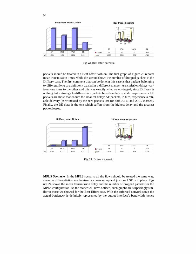
52

Best-effort: mean TX time

BE 0,251 0,25 0,251 0,249 EF AF11 AF12 DE

EF AF11 AF

12 DE

BE: dropped packets

dropped 99 185 3 453 sent 2807 3204 574 4724

EF AF11 AF12 DE

Fig. 22. Best effort scenario

packets should be treated in a Best Effort fashion. The first graph of Figure 23 reportsmean transmission times, while the second shows the number of dropped packets in theDiffserv case. The first comment that can be done in this case is that packets belongingto different flows are definitely treated in a different manner: transmission delays varyfrom one class to the other and this was exactly what we envisaged, since Diffserv isnothing but a strategy to differentiate packets based on their specific requirements. EFpackets are those that endure the smallest delay; AF packets, in turn, experience a reli-able delivery (as witnessed by the zero packets lost for both AF11 and AF12 classes).Finally, the DE class is the one which suffers from the highest delay and the greatestpacket losses.

DiffServ: mean TX time

DS 0,015 0,127 0,127 0,444 EF AF11 AF12 DE

EF AF11 AF

12 DE

DiffServ: dropped packets

dropped 11 0 0 769 sent 2807 3204 574 4725

EF AF11 AF12 DE

Fig. 23. Diffserv scenario

MPLS Scenario In the MPLS scenario all the flows should be treated the same way,since no differentiation mechanism has been set up and just one LSP is in place. Fig-ure 24 shows the mean transmission delay and the number of dropped packets for theMPLS configuration. As the reader will have noticed, such graphs are surprisingly sim-ilar to those we showed for the Best Effort case. With the enforced network setup theactual bottleneck is definitely represented by the output interface’s bandwidth, hence

53

the contribution due to packet processing is negligible when compared to the others:that is why we were not able to appreciate the performance difference between plain IPand MPLS we observed and measured in Sect. 2.

MPLS: mean TX time

MPLS 0,251 0,251 0,252 0,249 EF AF11 AF12 DE

EF AF11 AF

12 DE

MPLS: dropped packets

dropped 141 152 2 445 sent 2808 3204 574 4725

EF AF11 AF12 DE

Fig. 24. MPLS scenario

Diffserv over MPLS Scenario Let us finally take a look at the results obtained withthe last configuration, where Diffserv is running over an MPLS backbone. Figure 25shows how the presence of a Diffserv infrastructure meets the requirements for both EFand AF flows. By comparing the graphs in Figuer 23 with those in Figure 25 we noticethat the traffic profiles are almost the same in the two scenarios. If you are wonderingwhy MPLS should be used, since it adds little to network performance in the contextdescribed (i.e. one in which the routing tables dimensions are pretty small), rememberthat its major benefit is disclosed as soon as constraint-based routing techniques aretaken into account. Stated in different terms, a comparison based solely on the delayperformance figures is not fair, since a thorough analysis cannot avoid considering thefact that MPLS enables traffic engineering, by evading traditional (e.g. shortest path)forwarding, in favor of fully customized routing paradigms.

DS+MPLS: mean TX time

DS+MPLS 0,013 0,12 0,119 0,444 EF AF11 AF12 DE

EF AF11 AF

12 DE

DS+MPLS: dropped packets

dropped 10 0 0 774 sent 2807 3204 574 4724

EF AF11 AF12 DE

Fig. 25. DS+MPLS scenario

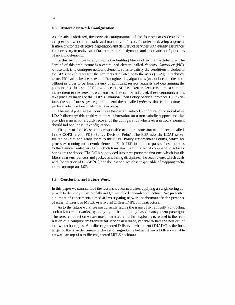
54

8.5 Dynamic Network Configuration

As already underlined, the network configurations of the four scenarios depicted inthe previous section are static and manually enforced. In order to develop a generalframework for the effective negotiation and delivery of services with quality assurance,it is necessary to realize an infrastructure for the dynamic and automatic configurationsof network elements.

In this section, we briefly outline the building blocks of such an architecture. The“brain” of this architecture is a centralized element called Network Controller (NC),whose task is to configure network elements so as to satisfy the conditions included inthe SLSs, which represent the contracts stipulated with the users (SLAs) in technicalterms. NC can make use of two traffic engineering algorithms (one online and the otheroffline) in order to perform its task of admitting service requests and determining thepaths their packets should follow. Once the NC has taken its decisions, it must commu-nicate them to the network elements, so they can be enforced; these communicationstake place by means of the COPS (Common Open Policy Service) protocol. COPS de-fines the set of messages required to send the so-called policies, that is the actions toperform when certain conditions take place.

The set of policies that constitutes the current network configuration is stored in anLDAP directory; this enables to store information on a non-volatile support and alsoprovides a mean for a quick recover of the configuration whenever a network elementshould fail and loose its configuration.

The part of the NC which is responsible of the transmission of policies is called,in the COPS jargon, PDP (Policy Decision Point). The PDP asks the LDAP serverfor the policies and sends them to the PEPs (Policy Enforcement Points), which areprocesses running on network elements. Each PEP, in its turn, passes these policiesto the Device Controller (DC), which translates them in a set of command to actuallyconfigure the device. The DC is subdivided into three parts: the first one, which installsfilters, markers, policers and packet scheduling disciplines; the second one, which dealswith the creation of E-LSP [91], and the last one, which is responsible of mapping trafficon the appropriate LSP.

8.6 Conclusions and Future Work

In this paper we summarized the lessons we learned when applying an engineering ap-proach to the study of state-of-the-art QoS-enabled network architectures. We presenteda number of experiments aimed at investigating network performance in the presenceof either Diffserv, or MPLS, or a hybrid Diffserv/MPLS infrastructure.

As to the future work, we are currently facing the issue of dynamically controllingsuch advanced networks, by applying to them a policy-based management paradigm.The research direction we are most interested in further exploring is related to the real-ization of a complex architecture for service assurance, capable to take the best out ofthe two technologies. A traffic-engineered Diffserv environment (TRADE) is the finaltarget of this specific research: the major ingredients behind it are a Diffserv-capablenetwork on top of a traffic-engineered MPLS backbone.

55

8.7 Acknowledgments

This work has been carried out partially under the financial support of the Ministerodell’Istruzione, dell’Universita e della Ricerca (MIUR) in the framework of the FIRBProject “Middleware for advanced services over large-scale, wired-wireless distributedsystems (WEB-MINDS)”

9 Wide Area Measurements of Voice Over IP Quality

It is well known that the users of real time voice services are sensitive and susceptibleto audio quality. If the quality deteriorates below an acceptable level or is too variable,users often abandon their calls and retry later. Since the Internet is increasingly beingused to carry real time voice traffic, the quality provided has become, and will remainan important issue. The aim of this work is therefore to disclose the current quality ofvoice communication at end-points on the Internet.

It is intended that the results of this work will be useful to many different com-munities involved with real time voice communication. Within the next paragraph welist some potential groups to whom this work might have relevance. Firstly end userscan determine which destinations are likely to yield sufficient quality. When deemedinsufficient they can take preventative measures such as adding robustness, for examplein the form of forward error correction to their conversations. Operators can use find-ings such as these to motivate upgrading links or adding QoS mechanisms where poorquality is being reported. Network regulators can use this kind of work to verify thequality level that was agreed upon, has indeed been deployed. Speech coder designerscan utilise the data as input for a new class of codecs, of particular interest are designswhich yield good quality in the case of bursty packet loss. Finally, researchers could usethe raw data we gathered to investigate questions such as, “is the quality of real timeaudio communication on the Internet improving or deteriorating?”.

The structure of the following sections are as follows: Section 9.1 begins with somebackground on the quality measures we have used in this work namely, loss, delayand jitter. Following on from the quality measures section 9.2 gives a description ofthe methodology used to ascertain the quality. In section 9.3 the results are presented,and due to space considerations we condense the results into one table showing thedelay, loss and jitter values for the paths we measured. In section 9.4 the related work isgiven, comparing results obtained in this attempt with other researchers’ work. This isconsidered important as it indicates whether quality has improved or deteriorated sincethose studies. Section 9.5 rounds off with some conclusions and a pointer to the datagathered.

9.1 What Do We Mean by Voice over IP Quality?

Ultimately, users judge the quality of voice transmissions. Organisations such as ETSI,ITU, TIA, RCR plus many others have detailed mechanisms to assess voice quality. Forthese organisations the particular focus is speech coders. Assigning quality “scores”involves replaying coded voice to both experienced and novice listeners and asking

56

them to state the perceived quality. Judging the quality of voice data that has beentransmitted across a wide area network is more difficult. The network inflicts its ownimpairment on the quality of the voice stream. By measuring the delay, jitter and lossof the incoming data stream at the receiver, we can provide some indication on howsuitable the network is for real time voice communication.

Therefore the quality of VoIP sessions can often be quantified by network delay,packet loss and packet jitter. We emphasise that these three quantities are the majorcontributors to the perceived quality as far as the network is concerned. The G.114 ITUstandard states the end-to-end one way delay should not exceed 150ms [100]. Delaysover this value adversely effect the quality of the conversation. In an alternative studyCole and Rosenbluth state that users perceive a linear degradation in the quality up to177ms [101]. Above this figure the degradation is also linear although markedly worse.As far as the packet loss is concerned using simple speech coding, e.g. A-law or � -law,tests have shown that the mean packet loss should not exceed 10% before glitches due tolost packets seriously affect the perceived quality. Note that a loss rate such as this doesnot say anything about the distribution of the losses. As far as the authors are aware of,no results exist that state how jitter solely can affect the quality of voice communication.When de-jittering mechanisms are employed, the network jitter is typically transferredinto application delay. The application must hold back a sufficient number of packetsin order to ensure smooth, uninterrupted playback of speech. To summarise, we referto the quality as a combination of delay, jitter and loss. It is important to mention weexplicitly do not state how these values should be combined. The ITU E-model [102] isone approach but others exist, therefore we refer the interested reader to the referencesin this section as well as [103] and [104].

9.2 Simulating and Measuring Voice over IP Sessions

Our method to measure VoIP quality is to send pre-recorded calls between globallydistributed sites. Through the modification of our own VoIP tool, Sicsophone, the in-tervening network paths are probed by a 70 second pre-recorded “test signal”. The goalof this work is therefore to report in what state the signal emerges after traversing thenetwork paths available to us. Incidentally, we do not include the signalling phase (i.e.establishing communication with the remote device) in these measurements, rather weconcentrate solely on the quality of the data transfer.

Nine sites have been carefully chosen with large variations in hops, geographic dis-tances, time zones and connectivity to obtain a diverse selection of distributed sites. Onelimitation of the available sites was they were all located at academic institutions, whichare typically associated with well provisioned networks. Their locations are shown inthe map of Figure 26. The sites were connected as a full mesh allowing us, in theory, tomeasure the quality of 72 different Internet paths. In practice, some of the combinationswere not usable due to certain ports being blocked, thus preventing the audio to be sentto some sites. There were four such cases. Bi-directional sessions were scheduled on anhourly basis between any two given end systems. Calls were only transferred once perhour due to load considerations on remote machines.

In Table 3 below we list the characteristics of the call we used to probe the Internetpaths between those indicated on the map. Their locations, separation in hops and time

57

Cooperating Sites in 1998Cooperating Sites in 2002

Fig. 26. The nine sites used in 2002 are shown with circles. The six depicted with squares showthose that were available to us in 1998, three remained unchanged during the past four years.

zones are given in the results section. As stated the call is essentially a fixed length PCMcoded file which can be sent between the sites, the length of the call and the payload sizewere arbitrarily chosen. Over a 15 week period we gathered just over 18,000 recordedsessions. The number of sessions between the nine sites is not evenly distributed due tooutages at some sites, however we attempted to ensure an even number of measurementsper site, in total nearly 33 million individual packets were received during this work.

A Networking Definition of Delay We refer to the delay as the one way network delay.One way delay is important in voice communication, particularly if it is not equal ineach direction. Measuring the one way delay of network connections without the useof synchronised clocks is a non-trivial task. Hence many methods rely on round-tripmeasurements and halve the result, hence estimating the one way delay. We measuredthe network delay using the RTCP protocol which is part of the RTP standard [105].A brief description follows. At given intervals the sender transmits a so called “report”containing the time the report was sent. On reception of this report the receiver recordsthe current time. Therefore two times are recorded within the report. When returningthe report to the sender, the receiver subtracts the time it put in the report, thereforeaccounting for the time it held the report. Using this information the sender can calculatethe round-trip delay and importantly, discount the time spent processing the reports atthe receiver. This can be done in both directions to see if any significant anomalies exist.We quote the network delay in the results section as they explicitly do not include anycontribution from the end hosts. Therefore it is important to state the delay is not theend-to-end delay but the network delay. We chose not to include the delay contributedby the end system as it varies widely from operating system to operating system and

58

Test “signal”Call duration 70 secondsPayload size 160 bytes

Packetisation time (ms) 20msData rate 64kbits/sec

With silence suppression 2043 packetsWithout silence suppression 3653 packets

Coding 8 bit PCMRecorded call size 584480 bytes

Obtained dataNumber of hosts used (2003) 9

Number of traces obtained 18054Number of data packets 32,771,021

Total data size (compressed) 411 MegabytesMeasurement duration 15 weeks

Table 3. The top half of the table gives details of the call used to measure the quality of linksbetween the sites. The lower half provides information about the data which we gathered.

how the VoIP application itself is implemented. The delay incurred by an end systemcan vary from 20ms up to 1000ms, irrespective of the stream characteristics.

Jitter - An IETF Definition Jitter is the statistical variance of the packet interarrivaltime. The IETF in RFC 1889 define the jitter to be the mean deviation (the smoothedabsolute value) of the packet spacing change between the sender and the receiver [105].Sicsophone sends packets of identical size at constant intervals which implies that( � ( �

(the sending times of two consecutive packets) is constant. The differenceof the packet spacing, denoted � , is used to calculate the interarrival jitter. Accordingto the RFC, the interarrival jitter should be calculated continuously as each packet � isreceived. For one particular packet the interarrival jitter �

� � � for the previous packet� � �

is calculated thus:

��

� � � � �� .

According to the RFC “the gain parameter 1/16 gives a good noise reduction ratiowhile maintaining a reasonable rate of convergence”. As stated earlier buffering dueto jitter adds to the delay of the application. This is therefore not visible in the resultswe present. The “real” time needed for de-jittering depends on how the original timespacing of the packets should be restored. For example if a single packet buffer is em-ployed it would result in an extra 20ms (the packetisation time) being added to the totaldelay. Note that packets arriving with a spacing greater than 20ms should be discardedby the application as being too late for replay. Multiples of 20ms can thus be allocatedfor every packet held before playout in this simple example.

Counting Ones Losses in the Network We calculate the lost packets as is exactlydefined in RFC 1889. It defines the number of lost packets as the expected number

59

of packets subtracted by the number actually received. The loss is calculated usingexpected values so as to allow more significance for the number of packets received,for example 20 lost packets from 100 packets has a higher significance than 1 from 5.For simple measures the percentage of lost packets from the total number of packetsexpected is stated. From above we know that the losses in this work do not includethose incurred by late arrivals, as knowledge of the buffer playout algorithm is needed,therefore our values are only the network loss. Detailed analysis of the loss patterns isnot given in the results section, we simply state the percentages of single, double andtriplicate losses.

9.3 Results

The results of 15 weeks of measurements are condensed into Figure 27. The tableshould be interpreted as an 11x11 matrix. The locations listed horizontally across thetop of the table are the locations configured as receivers, and when listed vertically theyare configured as senders. The values in the rightmost column and bottom row are thestatistical means for all the connections from the host in the same row and to the hostin the same column respectively. For example the last column of the first row (directlyunder Mean) the average delay to all destinations from Massachusetts is 112.8ms.

Each cell includes the delay, jitter, loss, number of hops and the time differencelisted vertically in the cell and prefixed by the letters D, J, L, H and T for each ofthe connections. The units for each quantity is the delay in milliseconds, the jitter inmilliseconds, the loss in percentage, the hops as reported by traceroute and time differ-ences in hours. A ‘+’ indicates that the local time from a site is ahead of the one in thecorresponding cell and behind for a ’-’. The values in parenthesis are the standard de-viations. A NA signifies “Not Available” for this particular combination of hosts. Thebottom rightmost cell contains the mean for all 18054 calls made, both to and fromall the nine hosts involved. The most general observation is the quality of the paths isgenerally good. The average delay is just below the ITU’s G.114 recommendation forthe end-to-end delay. Nevertheless at 136ms it does not leave much time for the endsystems encode/decode and replay the voice stream. A small buffer would absorb the4.1ms jitter and a loss rate of 1.8% is more than acceptable with PCM coding [103].

There are two clear groupings from these results, those within the EU and the USand those outside. The connections in Europe and the United States and between themare very good. The average delay between the US/EU hosts is 105ms, the jitter is 3.76msand the loss 1.16%. Those outside fair less well. The Turkish site suffers from large de-lays, which is not surprising as the Turkish research network is connected via a satellitelink to Belgium (using the Geant network). The jitter and loss figures however are low,5.7ms and 4% respectively. The Argentinian site suffers from asymmetry problems. Thequality when sending data to it is significantly worse than when receiving data from it.The delay is 1/3 higher, the jitter is more than twice as in the opposite direction andthe loss is nearly four times higher than when sending to it. Unfortunately we could notperform a traceroute from the host in Buenos Aires due to not having root access withwhich to run a traceroute like command, so we cannot say how the route contributed tothese values.

60receiverMassachusetts Michigan California Belgium Finland Sweden Germany Turkey Argentina Mean

senderD:38.0 (17.1) D:54.2 (15.8) D:67.1 (15.5) D:97.1 (2.6) D:99.5 (8.5) D:58.4 (5.0) D:388.2 (43.2) D:99.7 (4.9) D:112.8J:2.4 (1.7) J:2.4 (1.8) J:3.6 (1.5) J:2.5 (1.5) J:3.2 (1.7) J:4.5 (1.4) J:10.4 (4.9) J:19.9 (8.4) J:6.1

Massachusetts * L:0.1 (0.6) L:0.1 (0.9) L:0.1 (0.8) L:0.1 (0.8) L:0.04 (0.2) L:0.0 (0.0) L:4.9 (4.7) L:8.9 (7.2) L:1.2H:14 (+1) H:19 H:11 H:15 H:21 H:17 (+3) H:20 H:25 H:17T:0 T:-3 T:+6 T:+7 T:+6 T:+6 T:+7 T:+1

D:36.4 (15.4) D:40.4 (4.5) D:63.5 (4.2) D:88.2 (8.0) D:86.7 (4.7) D:63.6 (8.2) D:358.9 (44.9) D:112.1 (10.6) D:106.2J:4.7 (0.8) J:4.4 (0.8) J:4.3 (0.7) J:4.1 (0.7) J:5.2 (0.6) J:7.3 (1.9) J:5.6 (1.7) J:18.7 (7.9) J:6.8

Michigan L:0.0(0.2) * L:0.2 (1.1) L:0.0 (0.1) L:0.1 (1.1) L:0.1 (2.2) L:0.2 (0.9) L:3.0 (1.9) L:6.5 (7.0) L:1.3H:14 (+1) H:20 (+1) H:11 H:17 H:23 H:16 (+1) H:20 H:25 H:18T:0 T:-3 T:+6 T:+7 T:+6 T:6 T:7 T:+1D:54.5 (16.7) D:40.6 (5.1) D:81.0 (2.2) D:106.0 (3.0) D:108.0 (2.4) D:81.5 (1.8) D:386.9 (60.5) D:123.9 (12.4) D:122.2J:2.0 (1.0) J:1.2 (0.6) J:1.6 (0.8) J:1.4 (0.8) J:2.1 (0.9) J:4.9 (1.5) J:5.3 (1.7) J:18.1 (9.9) J:4.6

California L:0.1 (0.36) L:0.1 (1.9) * L:0.2 (0.8) L:0.6 (1.4) L:0.2 (0.3) L:2.8 (3.0) L:4.4 (2.4) L:8.9 (8.2) L:2.2H:18 (+1) H:21 H:20 H:25 (+1) H:30 (+2) H:23 H:23 H:25 H:23T:+3 T:+3 T:+9 T:+10 T:+9 T:+9 T:+10 T:+4D:65.2 (10.1) D:63.4 (3.3) D:84.0 (1.3) D:31.3 (0.6) D:33.4 (0.2) D:16.6 (10.4) D:341.1 (24.7) D:136.5 (7.1) D:96.4J:1.6 (0.6) J:0.6 (0.1) J:0.9 (0.8) J:0.9 (0.5) J:1.6 (0.9) J:3.4 (1.5) J:6.9 (2.0) J:NA J:2.0

Belgium L:0.0 (0.0) L:0.0 (0.0) L:1.2 (1.0) * L:0.0 (0.0) L:0.0(0.0) L:0.21 (0.7) L:3.8 (2.7) L:NA L:0.6H:16 H:17 H:23 H:17 H:22 H:13 H:16 (+2) H:19 H:17T:-6 T:-6 T:-9 T:+1 T:0 T:0 T:+1 T:-5D:97.8 (4.2) D:86.8 (1.9) D:109.9 (4.7) D:30.7 (0.3) D:13.6 (1.0) D:26.8 (7.3) D:321.2 (39.3) D:161.5 (12.2) D:106.3J:1.7 (0.8) J:1.1 (0.6) J:1.4 (0.8) J:1.4 (0.6) J:1.9 (0.9) J:3.9 (1.1) J:3.4 (1.7) J:17.4 (8.2) J:4.1

Finland L:0.0 (0.1) L:0.0 (0.3) L:0.7 (1.4) L:0.1 (0.3) * L:0.0 (0.0) L:0.0(0.0) L:3.2 (1.7) L:7.5 (6.5) L:1.4H:15 (+1) H:17 (+1) H:24 (+2) H:16 H:20 H:20 (+1) H:17 (+2) H:19 H:18T:-7 T:-7 T:-10 T:-1 T:-1 T:-1 T:0 T:-6

D:99.3 (8.8) D:84.9(1.9) D:105.6 (2.1) D:33.3 (0.4) D:13.5 (0.5) D:29.8 (12.8) D:322.2 (30.3) D:165.6 (17.9) D:107.8J:3.0 (1.9) J:2.5 (2.0) J:3.2 (1.96) J:2.8 (1.6) J:2.4 (1.8) J:4.8 (2.5) J:3.2 (1.49) J:NA J:2.8

Sweden L:0.0 (0.0) L:0.03 (0.4) L:0.1 (0.1) L:0.1 (0.3) L:0.0 (0.01) * L:0.0 (0.0) L:2.9 (1.0) L:NA L:0.4H:22 (+1) H:25 H:30 H:24 H:21 H:25 H:26 H:41 H:26T:-6 T:-6 T:-9 T:0 T:+1 T:0 T:+1 T:-5

D:63.5 (9.6) D:60.4 (0.5) D:84.4 (1.0) D:11.1 (0.2) D:27.8 (7.3) D:29.2 (7.6) D:300.7 (39.7) D:149.8 (15.6) D:90.9J:1.72 (0.7) J:0.7 (0.3) J:1.8 (0.7) J:0.8 (0.3) J:1.0 (0.5) J:1.5 (0.6) J:4.8 (2.1) J:NA J:1.6

Germany L:0.0(0.0) L:0.0 (0.0) L:2.5 (1.9) L:0.0 (0.0) L:0.0 (0.0) L:0.0 (0.0) * L:3.7 (2.5) L:NA L:0.8H:15 H:16 H:22 H:12 H:17 H:22 H:16 H:18 H:17T:-6 T:-6 T:-9 T:0 T:+1 T:0 T:+1 T:-5D:379.1 (47.1) D:387.9 (35.5) D:410.9 (43.9) D:330.2 (28.6) D:318.9 (42.4) D:311.1 (8.3) D:378.2 (49.3) D:490.8 (26.0) D:375.9J:8.6 (0.7) J:8.9 (1.2) J:8.8 (2.5) J:9.2 (2.0) J:8.8 (0.6) J:9.1 (0.7) J:10.7 (1.2) J:NA J:8.0

Turkey L:8.1 (2.8) L:8.0 (2.9) L:7.6 (6.8) L:7.10 (4.0) L:7.8 (2.7) L:8.4 (3.1) L:8.0 (3.1) * L:NA L:6.9H:18 (+1) H:20 H:19 H:17 H:19 H:25 H:16 H:18 H:19T:-7 T:-7 T:-10 T:-1 T:0 T:-1 T:-1 T:-6D:117.0 (30.8) D:146.7 (44.2) D:152.0 (47.8) D:NA D:164.1 (27.2) D:160.9 (47.7) D:180.5 (50.5) D:NA D:115.2J:4.2 (2.0) J:4.3 (2.3) J:3.1 (2.4) J:4.2 (2.0) J:3.9(2.2) J:2.9 (0.8) J:4.7 (1.5) J:6.0(1.2) J:4.2

Argentina L:0.5 (1.4) L:0.5 (1.5) L:0.6 (1.8) L:0.5 (1.4) L:0.5 (1.4) L:0.0 (0.1) L:0.1 (0.1) L:5.8 (3.0) * L:1.1H:NA H:NA H:NA H:NA H:NA H:NA H:NA H:NA H:NAT:-1 T:-1 T:-4 T:+5 T:+6 T:+5 T:+5 T:+6

D:114.1 D:113.6 D:115.7 D:77.1 D:105.8 D:105.2 D:104.4 D:345.6 D:180.0 D:136.2Mean J:3.4 J:3.4 J:3.2 J:3.5 J:3.1 J:3.4 J:5.5 J:5.7 J:9.3 J:4.1

L:1.1 L:1.1 L:1.6 L:1.0 L:1.1 L:1.1 L:1.4 L:4.0 L:4.00 L:1.8H:14 H:16 H:19 H:13 H:16 H:20 H:16 H:17 H:23 H:18

Fig.27.A

summ

aryof18000

VoIP

sessions.The

delay,jitterandloss

forthenine

sites.The

delayand

jitterare

inm

illiseconds,thelosses

arein

percentages.T

henum

berof

hopsand

time

zones(in

hours)are

alsogiven.T

hem

eansfor

eachsite

andallsites

arestated

andstandard

deviationsare

inparenthesis.

61

We now turn our attention to results which are not related to any particular site.As far as loss is concerned the majority of losses are single losses. 78% of all thelosses counted in all trace files were single losses whereas 13% were duplicate lossesand only 4% triplicate losses. Generally the jitter is low relative to the delay of thelink, approximately 3-4%. This is not totally unexpected as the loss rates are also low.With the exception of the Argentinian site, the sites did not exhibit large differences inasymmetry and were normally within 5% of each other in each direction. It is interestingto note that the number of hops could vary under the 15 week measurement perioddenoted by () in the hops field. Only very few ( � � � � �

��) out of sequence packets were

observed. Within [106] there are details of other tests, such as the effect of using silencesuppression, differing payload sizes and daytime effects. In summary no significantdifferences were observed as these quantities were varied.

9.4 Related Work

Similar but less extensive measurements were performed in 1998 [107]. Only three ofthe hosts remain from four years ago so comparisons can only be made for these routes.An improvement, in the order of 5-10% has been observed for these routes. We shouldpoint out though, the number of sessions recorded four years ago numbered only tensper host, whereas on this occasion we performed hundreds of calls from each host.Bolot et. al. looked at consecutive loss for a FEC scheme [108]. They concluded thatthe number of consecutive losses is quite low and stated that most losses are one tofive losses at 8am and between one to ten at 4pm. This is in broad agreement withthe findings in this work, however we did not investigate the times during the day ofthe losses. Maxemchuk and Lo measured both loss and delay variation for intra-stateconnections within the USA and international links [109]. Their conclusion was thequality depends on the length of the connection and the time of day. We did not trydifferent length of connections but saw much smaller variations (almost negligible)during a 24 hour cycle (see [106]). We attribute this to the small 64kbits per second VoIPsession on well dimensioned academic networks. It is worthy to point out our loss rateswere considerably less than Maxemchuks (3-4%). Dong Lin had similar conclusions[110], stating that in fact even calls within the USA could suffer from large jitter delays.Her results on packet loss also agree with those in [108], which is interesting, as themeasurements were taken some four years later.

9.5 Conclusions

We have presented the results of 15 weeks of voice over IP measurements consisting ofover 18000 recorded VoIP sessions. We conclude that the quality of VoIP is very goodand in most cases is over the requirements as stated in many speech quality recommen-dations. Recall that all of the sites were at academic institutions which is an importantfactor when interpreting these results as most universities have well provisioned links,especially to other academic sites. Nevertheless, the loss, delay and jitter values arevery low and from previous measurements the quality trend is improving. We can onlyattribute this to more capacity and better managed networks than those four years ago.However some caution should be expressed as the sample period was only 15 weeks, the

62

bandwidth of the flows very small and only used once per hour. We do have howeverquite a large number of sample sessions. VoIP is dependent on the IP network infra-structure and not only on the geographic distance. This can be clearly seen in the differ-ences between the Argentinian and Turkish hosts. We have found performing measure-ments on this scale is not an easy task. Different access mechanisms, firewalls, NATsand not having super-user permission complicates the work in obtaining measurements.Since it is not possible to envisage all the possible uses for this data we have made itavailable for further investigation at http://www.sics.se/˜ianm/COST263/cost263.html.

References

1. Willinger, W., Paxson, V.: Where mathematics meets the internet. Notices of the AmericanMathematical Society 45 (1998) 961–970

2. Park, K., Willinger, W.: Self-similar network traffic and performance evaluation. Wiley(2000)

3. Padhye, J., Firoiu, V., Towsley, D., Kurose, J.: Modeling tcp throughput: a simple modeland its empirical validation. In: Proceedings of SIGCOMM 98, ACM. (1998)

4. Kleinrock, L.: Queuing Theory - Vol 2. Wiley (1976)5. Ben Fredj, S., Bonald, T., Proutire, A., Rgni, G., Roberts, J.: Statistical bandwidth sharing:

a study of congestion at flow level. Proceedings of Sigcomm 2001, Computer Communi-cation Review 31 (2001) 111–122

6. Bonald, T., Roberts, J.: Congestion at flow level and the impact of user behaviour. ComputerNetworks, to appear (2003)

7. Le Boudec, J.Y., Thiran, P.: A theory of deterministic queuing systems for the Internet.Volume 2050 of Lecture notes in computer science. Springer-Verlag (2001)

8. Bonald, T., Proutire, A., Roberts, J.: Statistical performance guarantees for streaming flowsusing expedited forwarding. In: Proceedings of Infocom 2001. (2001) 1104–1112

9. Gibbens, R., Kelly, F., Key, P.: A decision theoretic approach to call admission control.IEEE JSAC 13 (1995) 1104–1114

10. Bonald, T., Oueslati, S., Roberts, J.: Ip traffic and qos control: towards a flow-aware archi-tecture. In: Proceedings of World Telecom Conference, Paris (2002)

11. Benameur, N., Ben Fredj, S., Delcoign, F., Oueslati-Boulahia, S., Roberts, J.: Integratedadmission control for streaming and elastic flows. In: Proceedings of QofIS 2001, LNCS2156, Springer (2001)

12. Quadros, G., Monteiro, E., Boavida, F.: A qos metric for packet networks. In: Proceed-ings of SPIE International Symposium on Voice, Video, and Data Communications, HynesConvention Center, Boston, Massachusetts, USA (1998)

13. for Standardization, I.O.: Information technology – quality of service: Framework. Inter-national Standard 13236 (1998)

14. Blake, S., Black, D., Carlson, M., Davies, E., Wang, Z., Weiss, W.: Rfc 2475 – an architec-ture for differentiated service (1998)

15. Quadros, G., Alves, A., Monteiro, E., Boavida, F.: An approach to support traffic classes inip networks. In Crowcroft, J., Roberts, J., Smirnov, M.I., eds.: Lecture Notes in ComputerScience. Volume 1922., Berlin, Germany, Springer-Verlag, Heidelberg (2000) 285–299

16. Quadros, G., Alves, A., Monteiro, E., Boavida, F.: An effective scheduler for ip routers.In: Proceedings of ISCC’2000, Antibes, France, Fifth IEEE Symposium on Computers andCommunications (2000)

63

17. Quadros, G., Alves, A., Silva, J., Matos, H., Monteiro, E., Boavida, F.: A queue manage-ment system for differentiated-services ip routers. In Crowcroft, J., Roberts, J., Smirnov,M.I., eds.: Lecture Notes in Computer Science. Volume 1922., Berlin, Germany, Springer-Verlag, Heidelberg (2000) 14–27

18. Alves, A., Quadros, G., Monteiro, E., Boavida, F.: Qostat – a tool for the evaluation ofqos-capable routers. In: Proceedings of SPIES’s International Symposium on Voice, Video,and Data Communications, Boston (2000)

19. netIQ: Chariot – User Guide. (2001)20. Oliveira, M., Brito, J., Melo, B., Quadros, G., Monteiro, E.: Encaminhamento com qual-

idade de servico: Desafios da implementacao da estrategia qosr-lct (portuguese). In: Pro-ceedings of CRC’2000, Third National Conference on Computer Networks – Technologiesand Applications, Viseu, Portugal, FCCN (2000)

21. Oliveira, M., Melo, B., Quadros, G., Monteiro, E.: Quality of service routing in the dif-ferentiated services framework. In: Proceedings of SPIES’s International Symposium onVoice, Video, and Data Communications, Boston (2000)

22. Lourenco, D., Oliveira, M., Quadros, G., Monteiro, E.: Definicao do mecanismo de con-trolo de admissao para o modelo de servicos de lct-uc. In: Proceedings of CRC’2000, ThirdNational Conference on Computer Networks – Technologies and Applications, Viseu, Por-tugal, FCCN (2000)

23. Breslau, L., Shenker, S.: Best–effort versus reservations: A simple comparative analysis.ACM Computer Communication Review 28 (1998) 3–16

24. Braden, R., Clark, S., Shenker, S.: Integrated services in the internet architecture. RFC1633, IETF (1994)

25. Blake, S., Black, D., Carlson, M., Davies, E., Wang, Z., Weiss, W.: An architecture fordifferentiated services. RFC 2475, IETF (1998)

26. Shenker, S., Partridge, C., Guerin, R.: Specification of guaranteed quality of service. RFC2212, IETF (1997)

27. Wroclawski, J.: Specification of the controlled-load network element service. RFC 2211,IETF (1997)

28. Braden, R., Zhang, L., Berson, S., Herzog, S., Jamin, S.: Resource ReSerVation protocol(RSVP). RFC 2205, IETF (1997)

29. Jacobson, V., Nichols, K., Poduri, K.: An expedited forwarding PHB. RFC 2598, IETF(1999)

30. Heinanen, J., Baker, F., Weiss, W., Wroclawski, J.: Assured forwarding PHB group. RFC2597, IETF (1999)

31. Baker, F., Iturralde, C., Le Faucheur, F., Davie, B.: RSVP reservations aggregation. InternetDraft, IETF (2001) (Work in progress).

32. Bernet, Y.: Format of the RSVP DCLASS object. RFC 2996, IETF (2000)33. Bernet, Y., Ford, P., Yavatkar, R., Baker, F., Zhang, L., Speer, M., Braden, R., Davie, B.,

Wroclawski, J., Felstaine, E.: A framework for integrated services operation over diffservnetworks. RFC 2998, IETF (2000)

34. Cetinkaya, C., Knightly, E.W.: Egress admission control. In: Proc. of IEEE INFOCOM2000, Tel Aviv, Israel (2000) 1471–1480

35. Breslau, L., Jamin, S., Shenker, S.: Comments on the performance of measurement–basedadmission control algorithms. In: Proc. of IEEE INFOCOM 2000, Tel Aviv, Israel (2000)1233–1242

36. Karlsson, G.: Providing quality for internet video services. In: Proc. of CNIT/IEEE IT-WoDC 98, Ischia, Italy (1998) 133–146

37. Fodor (nee Elek), V., Karlsson, G., Ronngren, R.: Admission control based on end-to-endmeasurements. In: Proc. of IEEE INFOCOM 2000, Tel Aviv, Israel (2000) 623–630

64

38. Ramakrishnan, K., Floyd, S.: A proposal to add explicit congestion notification (ECN) toIP. RFC 2481, IETF (1999)

39. Kelly, F.P., Key, P.B., Zachary, S.: Distributed admission control. IEEE Journal on SelectedAreas in Communications 18 (2000) 2617–2628

40. Kelly, T.: An ECN probe–based conection acceptance control. ACM Computer Communi-cation Review 31 (2001) 14–25

41. Bianchi, G., Capone, A., Petrioli, C.: Throughput analysis of end–to–end measurement-based admission control in IP. In: Proc. of IEEE INFOCOM 2000, Tel Aviv, Israel (2000)1461–1470

42. Bianchi, G., Capone, A., Petrioli, C.: Packet management techniques for measurementbased end-to-end admission control in IP networks. Journal of Communications and Net-works 2 (2000) 147–156

43. Bianchi, G., Borgonovo, F., Capone, A., Petrioli, C.: Endpoint admission control with delayvariation measurements for QoS in IP networks. ACM Computer Communication Review32 (2002) 61–69

44. Breslau, L., Knightly, E.W., Shenker, S., Stoica, I., Zhang, H.: Endpoint admission control:Architectural issues and performance. In: Proc. of ACM SIGCOMM 2000, Stockholm,Sweden (2000) 57–69

45. Mas Ivars, I., Karlsson, G.: PBAC: Probe–based admission control. In: Proc. of QoFIS2001, Coimbra, Portugal (2001) 97–109

46. Mas, I., Fodor, V., Karlsson, G.: Probe–based admission control for multicast. In: Proc. ofIWQoS 02, Miami Beach, Florida (2002) 97–109

47. Gibbens, R.J., Kelly, F.P.: Distributed connection acceptance control for a connection-less network. In: Proc. of the 16th International Teletraffic Congress, Edinburgh, Scotland(1999) 941–952

48. Bianchi, G., Borgonovo, F., Capone, A., Fratta, L., Petrioli, C.: PCP: an end-to-endmeasurement-based call admission control for real-time services over IP networks. In:Proc. of QoS–IP 2001, Rome, Italy (2001) 391–406

49. Roberts, J.W., Mocci, U., Virtamo, J., eds.: COST 242: Broadband Network Teletraffic.Volume 1155 of Lecture notes in computer science. Springer–Verlag (1996)

50. Conte, M., Mas, I., Fodor, V., Karlsson, G.: Policy enforcing for probe–based admissioncontrol. In: Proc. of NTS 16, Espoo, Finland (2002) 45–55

51. Ventre, G., et al.: Quality of Service control in Premium IP networks. Deliverable 2.1, ISTProject CADENUS — IST 11017 (2001)

52. Smirnov, M., et al.: SLA Networks in Premium IP. Deliverable 1.1, IST Project CADENUS— IST 11017 (2001)

53. Quittek, J., Zseby, T., Claise, B.: Requirements for IP Flow Information Export. InternetDraft, IETF (2002) (Work in progress).

54. ebXML Technical Architecture Project Team: ebXML Technical Architecture Specificationv.1.0.4. Technical specification, ebXML Consortium (2001)

55. D’Antonio, S., Fadini, B., Romano, S., Ventre, G.: Designing Service Negotiation Entitiesfor the Electronic Marketplace. In: Proceedings of SEKE2002, Ischia, Napoli — Italy(2002)

56. Cremonese, P., et al.: A Framework for Policy-based Management of QoS-aware IP Net-works. In: Proceedings of Networking2002, Pisa — Italy (2002)

57. Chan, K., et al.: COPS Usage for Policy Provisioning (COPS-PR). RFC 3084, IETF (2001)58. Rawlins, D., et al.: Framework of COPS-PR Policy Usage Feedback. Internet Draft, IETF

(2002) (Work in progress).59. Zhang, Z., Towsley, D., Kurose, J.: Statistical analysis of the generalized processor sharing

scheduling discipline. In Proceedings of ACM SIGCOMM (1994) 68–77

65

60. Zhang, Z., Liu, Z., Kurose, J., Towsley, D.: Call admission control schemes under general-ized processor sharing scheduling. The Journal of Telecommunication Systems, Modeling,Analysis, Design, and Management 7 (1997)

61. Elwalid, A., Mitra, D.: Design of generalized processor sharing schedulers which statisti-cally multiplex heterogeneous qos classes. In Proceedings of IEEE INFOCOM ’99 (1999)1220–1230

62. Parekh, A., Gallager, R.G.: A generalized processor sharing approach to flow control in in-tegrated services networks: The single-node case. IEEE/ACM Transactions on Networking1 (1993) 344–357

63. Parekh, A., Gallager, R.G.: A generalized processor sharing approach to flow control inintegrated services networks: The multiple node case. IEEE/ACM Transactions on Net-working 2 (1994) 137–150

64. Szabo, R., Barta, P., Nemeth, F., Biro, J.: Call admission control in generalized processorsharing (gps) schedulers using non-rate proportional weighting of sessions. In Proceedingsof INFOCOM ’00 (2000)

65. Zhang, Z., Liu, Z., Towsley, D.: Closed-form deterministic end-to-end performance boundsfor the generalized processor sharing scheduling discipline. Journal of Combinatorial Op-timization 1 (1998)

66. Georgiadis, L., Gu’erin, R., Peris, V., Sivarajan, K.: Efficient network qos provisioningbased on per node traffic shaping. IEEE/ACM Transactions on Networking 4 (1996) 482–501

67. Duffield, N.G., Lakshman, T.V., Stiliadis, D.: On adaptive bandwidth sharing with rateguarantees. In Proceedings of INFOCOM ’98 (1998) 1122–1130

68. Chang, C.S., Chen, K.C.: Service curve proportional sharing algorithm for service-guaranteed multiaccess in integrated-service distributed networks. In Proceedings ofGLOBECOM ’99 (1999) 1340 –1344

69. Stamoulis, A., Giannakis, G.: Deterministic time-varying packet fair queueing for inte-grated services networks. In Proceedings of GLOBECOM ’00 (2000) 621–625

70. Toutain, F.: Decoupled generalized processor sharing: A fair queueing principle for adaptivemultimedia applications. In Proceedings of INFOCOM ’98 (1998) 291–298

71. Panagakis, A., Stavrakakis, I.: Optimal call admission control under generalized processorsharing scheduling. In Proceedings of IWQoS ’01 (2001)

72. Boudec, J.Y.L.: Application of network calculus to guaranteed service networks. IEEETransactions on Information Theory 44 (1998) 1087–1096

73. Panagakis, A., Stavrakakis, I.: Generalized processor sharing enhancement through sessiondecomposition. In Proceedings of Net-Con ’02 (2002)

74. Sisodia, G., Headley, M.: Statistical analysis and simulation study of vbr coded videosource models in atm networks. In: Proceedings of UPC. (1998) 177–181

75. Li, S.Q., Hwang, C.L.: Queue response to input correlation functions: discrete spectralanalysis. IEEE Trans. on Networking 1 (1997) 533–552

76. Lombardo, A., Morabito, G., Schembra, G.: An accurate and treatable markov model ofmpeg video traffic. In: Proc. of IEEE INFOCOM 1998. (1998) 217–224

77. MPEG traces archive: (http://www-info3.informatik.uni-wuerzburg.de/mpeg/traces/)78. Heyman, D.: The gbar source model for vbr videoconferences. IEEE Trans. on Networking

5 (1997) 554–56079. Heyman, D., Tabatabai, A., Lakshman, T.: Statistical analysis and simulation study of video

teleconference traffic in atm networks. IEEE Trans. on Circ. and Syst. for Video Tech. 2(1992) 49–59

80. Koucheryavy, Y., Moltchanov, D., Harju, J.: A novel two-step mpeg traffic modeling algo-rithm based on a gbar process. In: Proc. of NET-CON. (2002) 293–304

66

81. Lombardo, A., Morabito, G., Palazzo, S., Schembra, G.: Intra-gop modeling of mpeg videotraffic. In: Proc. of IEEE ICC. Volume 1. (1998) 563–567

82. Lombardo, A., Morabito, G., Palazzo, S., Schembra, G.: A fast simulation of mpeg videotraffic. In: Proc. GLOBECOM. Volume 2. (1998) 702–707

83. Blondia, C., Casals, O.: Performance analysis of statistical multiplexing of vbr sources. In:Proc. IEEE INFOCOM. (1992) 828–838

84. Koucheryavy, Y., Moltchanov, D., Harju, J.: A top-down approach to vod traffc transmissionover diffserv domain using the af phb class. In: Proc. of IEEE ICC, Alaska, USA (2003)

85. Meyer, C.: Matrix analysis and applied linear algebra. SIAM Publications (2000)86. Hajek, B., Linhai, H.: On variations of queue response for inputs with the same mean and

autocorrelation function. IEEE Trans. on Networking 6 (1998) 588–59887. Awduche, D.: MPLS and Traffic Engineering in IP networks. IEEE Communications

Magazine 37 (1999) 42–4788. Rosen, E., Viswanathan, A., Callon, R.: Multiprotocol label switching architecture. RFC

3031, IETF (2001)89. Awduche, D., Chiu, A., Elwalid, A., Widjaja, I., Xiao, X.: Overview and Principles of

Internet Traffic Engineering. RFC 3272, IETF (2002)90. Blake et al., S.: An architecture for differentiated services. RFC 2475, IETF (1998)91. Le Faucheur et al., F.: Multi-protocol label switching (MPLS) support of differentiated

services. RFC 3270, IETF (2002)92. Cho, K.: Alternate Queuing (ALTQ) module, (http://www.csl.sony.co.jp/person/kjc/programs.html)93. Almesberger, W.: Linux network traffic control - implementation overview. White paper,

EPFL ICA (2001)94. Almesberger, W., Hadi Salim, J., Kuznetsov, A.: Differentiated services on linux. Internet

Draft, IETF (1999) (Work in progress).95. Leu, J.R.: MPLS for Linux, (http://sourceforge.net/projects/mpls-linux)96. Avallone, S., Esposito, M., Pescape, A., Romano, S., Ventre, G.: Measuring MPLS over-

head. In: Proc. of ICCC2002, Mumbai, India (2002)97. Avallone, S., D’Arienzo, M., Esposito, M., Pescape, A., Romano, S., Ventre, G.: Mtools.

IEEE Network 16 (2002) 3 Networking column.98. Avallone, S., Esposito, M., Pescape, A., Romano, S., Ventre, G.: Mtools: a one-way delay

and round-trip time meter. In Mastorakis, N., Mladenov, V., eds.: Recent Advances inComputers, Computing and Communications. (2002)

99. Avallone, S., Esposito, M., Pescape, A., Romano, S., Ventre, G.: An experimental analysisof Diffserv-MPLS interoperability. In: Proc. of ICT 2003, Papeete, French Polynesia (2003)

100. Recommendation G.114, I.T.: General Characteristics of International Telephone Connec-tions and International Telephone Circuits: One-Way Transmission Time (1998)

101. Cole, R., Rosenbluth, J.: Voice over IP Performance Monitoring. ACM Computer Commu-nication Review (2002)

102. ITU-T Recommendation G.107: The E-Model, a computational model for use in transmis-sion planning (1998)

103. L.F.Sun, G.Wade, B., E.C.Ifeachor: Impact of Packet Loss Location on Perceived SpeechQuality. In: Proceedings of 2nd IP-Telephony Workshop (IPTEL ’01), Columbia University,New York (2001) 114–122

104. Kitawaki, N., Kurita, T., Itoh, K.: Effects of Delay on Speech Quality. NTT Review 3(1991) 88–94

105. Schulzrinne, H., Casner, S., Frederick, R., Jacobson, V.: RTP: A Transport Protocol forReal-Time Applications. RFC 1889, Internet Engineering Task Force (1996)http://www.rfc-editor.org/rfc/rfc1889.txt.

106. Li, F.: Measurements of Voice over IP Quality. Master’s thesis, KTH, Royal Institute ofTechnology, Sweden (2002)

67

107. Hagsand, O., Hansson, K., Marsh, I.: Measuring Internet Telephone Quality: Where arewe today ? In: Proceedings of the IEEE Conference on Global Communications (GLOBE-COM), Rio, Brazil, IEEE (1999)

108. Bolot, J., Crepin, H., Garcia, A.: Analysis of audio packet loss in the internet. In: Proc. Inter-national Workshop on Network and Operating System Support for Digital Audio and Video(NOSSDAV). Lecture Notes in Computer Science, Durham, New Hampshire, Springer(1995) 163–174

109. Maxemchuk, N.F., Lo, S.: Measurement and interpretation of voice traffic on the Inter-net. In: Conference Record of the International Conference on Communications (ICC),Montreal, Canada (1997)

110. Lin, D.: Real-time voice transmissions over the Internet. Master’s thesis, Univ. of Illinoisat Urbana-Champaign (1999)

Traffic Management

Documents

Transcript of Traffic Management