Advanced Data Centre Traffic Management on Programmable ...
122
Faculty of Engineering, Computer Science and Psychology Institute of Information Resource Management November 2018 Advanced Data Centre Traffic Management on Programmable Ethernet Switch Infrastruc- ture Master thesis at Ulm University Submitted by: Kamil Tokmakov Examiners: Prof. Dr.-Ing. Stefan Wesner Prof. Dr. rer. nat. Frank Kargl Supervisor: M.Sc. Mitalee Sarker
-
Upload
khangminh22 -
Category
Documents
-
view
1 -
download
0
Transcript of Advanced Data Centre Traffic Management on Programmable ...

Faculty of
Engineering, Computer
Science and Psychology
Institute of Information
Resource Management
November 2018
Advanced Data Centre Traffic Managementon Programmable Ethernet Switch Infrastruc-tureMaster thesis at Ulm University
Submitted by:Kamil Tokmakov
Examiners:Prof. Dr.-Ing. Stefan WesnerProf. Dr. rer. nat. Frank Kargl
Supervisor:M.Sc. Mitalee Sarker

c© 2018 Kamil TokmakovThis work is licensed under the Creative Commons Attribution-NonCommercial-ShareAlike 4.0 License. Toview a copy of this license, visit https://creativecommons.org/licenses/by-nc-sa/4.0/deed.de.Composition: PDF-LATEX 2ε

Abstract
As an infrastructure to run high performance computing (HPC) applications, which representparallel computations to solve large problems in science or business, cloud computing offers tothe tenants an isolated virtualized infrastructure, where these applications span across multipleinterconnected virtual machines (VMs). Such infrastructure allows to rapidly deploy and scalethe amount of VMs in use due to elastic and virtualized resource share, such as CPU cores,network and storage, and hence provides feasible and cost-effective solution compared to abare-metal deployment. HPC VMs are communicating among themselves, while running theHPC applications. However, communication performance degrades with the use of the networkresources by other tenants and their services, because cloud providers often use cheap Ethernetinterconnect in their infrastructure, which operates on a best-effort basis and affects overallperformance of the HPC applications. Due to the limitations in virtualization and cost, lowlatency network technologies, such as Infiniband and Omnipath, cannot be directly introduced toimprove network performance, hence, appropriate traffic management needs to be applied forlatency-critical services like HPC in the Ethernet infrastructure.
This thesis work proposes the traffic management for an Ethernet-based cloud infrastructure,such that HPC traffic is prioritized and has better treatment in terms of lower latency and highershare of bandwidth compared to regular traffic. As a proof-of-concept, such traffic management isimplemented on the P4 software switch, bmv2, using rate limited strict priority packet schedulingto enable prioritization for HPC traffic, deficit round robin algorithm to enable scalable utilizationof available network resources and metadata-based interface to introduce programmability of thetraffic management via standard control plane commands.
The performance of the proposed traffic management is evaluated in mininet simulation environ-ment by comparing it with the best-effort approach and when only rate limited strict priorityscheduling is applied. The results of the evaluation demonstrate that the traffic managementprovides higher bandwidth and lower one-way and MPI ping-pong latencies than the best-effortapproach and has worse latency characteristics than strict priority scheduling, but trades offthe scalability in dynamic bandwidth allocation. Therefore, this thesis requires a future workto be done to further decrease the latency and subsequently, the evaluation on a real hardwareenvironment.
iii

iv

Declaration
I, Kamil Tokmakov, declare that I wrote this thesis independently and I did not use any othersources or tools than the ones specified.
Ulm, 29. November 2018.
Kamil Tokmakov
v

vi

Contents
1 Introduction 1
2 Background 52.1 High performance computing . . . . . . . . . . . . . . . . . . . . . . . . . . . . . . . 52.2 Cloud computing . . . . . . . . . . . . . . . . . . . . . . . . . . . . . . . . . . . . . . 62.3 Virtualization . . . . . . . . . . . . . . . . . . . . . . . . . . . . . . . . . . . . . . . . 72.4 Ethernet interconnection on clouds . . . . . . . . . . . . . . . . . . . . . . . . . . . . 82.5 Cloud data center infrastructure with Ethernet . . . . . . . . . . . . . . . . . . . . . 92.6 Analysis of HPC improvements in Ethernet-based clouds . . . . . . . . . . . . . . 112.7 SDN . . . . . . . . . . . . . . . . . . . . . . . . . . . . . . . . . . . . . . . . . . . . . . 152.8 Traffic Management . . . . . . . . . . . . . . . . . . . . . . . . . . . . . . . . . . . . . 19
2.8.1 Traffic policing and traffic shaping . . . . . . . . . . . . . . . . . . . . . . . . 192.8.2 Packet scheduling . . . . . . . . . . . . . . . . . . . . . . . . . . . . . . . . . 20
2.9 Traffic management with SDN . . . . . . . . . . . . . . . . . . . . . . . . . . . . . . 222.10 MPI communication . . . . . . . . . . . . . . . . . . . . . . . . . . . . . . . . . . . . 242.11 MPI traffic consideration over Ethernet . . . . . . . . . . . . . . . . . . . . . . . . . 262.12 Related work . . . . . . . . . . . . . . . . . . . . . . . . . . . . . . . . . . . . . . . . . 26
3 Proposed traffic management 293.1 Design requirements . . . . . . . . . . . . . . . . . . . . . . . . . . . . . . . . . . . . 293.2 Utilization concerns . . . . . . . . . . . . . . . . . . . . . . . . . . . . . . . . . . . . . 303.3 Traffic manager programmability . . . . . . . . . . . . . . . . . . . . . . . . . . . . . 343.4 Design discussion . . . . . . . . . . . . . . . . . . . . . . . . . . . . . . . . . . . . . . 343.5 Traffic manager behavior . . . . . . . . . . . . . . . . . . . . . . . . . . . . . . . . . . 35
4 Implementation 374.1 bmv2 switch . . . . . . . . . . . . . . . . . . . . . . . . . . . . . . . . . . . . . . . . . 37
4.1.1 bmv2 architecture . . . . . . . . . . . . . . . . . . . . . . . . . . . . . . . . . 374.1.2 bmv2 control plane . . . . . . . . . . . . . . . . . . . . . . . . . . . . . . . . . 384.1.3 bmv2 traffic management engine . . . . . . . . . . . . . . . . . . . . . . . . . 39
4.2 bmv2 extension stages . . . . . . . . . . . . . . . . . . . . . . . . . . . . . . . . . . . 404.2.1 Strict priority and rate limitation in bytes per second . . . . . . . . . . . . . 414.2.2 Rate limited strict priority with DRR . . . . . . . . . . . . . . . . . . . . . . 42
4.3 Metadata-based traffic management programmability . . . . . . . . . . . . . . . . . 454.4 Implementation notes . . . . . . . . . . . . . . . . . . . . . . . . . . . . . . . . . . . 45
5 Validation and performance implications 475.1 Bandwidth distribution and CPU consumption . . . . . . . . . . . . . . . . . . . . 475.2 Queue delays and buffers occupancy . . . . . . . . . . . . . . . . . . . . . . . . . . 48

Contents
6 Evaluation setup 536.1 Setup and tools . . . . . . . . . . . . . . . . . . . . . . . . . . . . . . . . . . . . . . . 53
6.1.1 Mininet . . . . . . . . . . . . . . . . . . . . . . . . . . . . . . . . . . . . . . . . 536.1.2 iperf . . . . . . . . . . . . . . . . . . . . . . . . . . . . . . . . . . . . . . . . . 546.1.3 MPICH . . . . . . . . . . . . . . . . . . . . . . . . . . . . . . . . . . . . . . . . 54
6.2 Test cases . . . . . . . . . . . . . . . . . . . . . . . . . . . . . . . . . . . . . . . . . . . 556.3 Evaluation model . . . . . . . . . . . . . . . . . . . . . . . . . . . . . . . . . . . . . . 576.4 Emulated topologies . . . . . . . . . . . . . . . . . . . . . . . . . . . . . . . . . . . . 62
6.4.1 TOPO-1: Topology-1, star . . . . . . . . . . . . . . . . . . . . . . . . . . . . . 636.4.2 TOPO-2: Topology-2, tree (depth=1) . . . . . . . . . . . . . . . . . . . . . . . 646.4.3 TOPO-3: Topology-3, tree (depth=2) . . . . . . . . . . . . . . . . . . . . . . . 68
7 Evaluation results 717.1 RUNTIME test case . . . . . . . . . . . . . . . . . . . . . . . . . . . . . . . . . . . . . 717.2 PROACTIVE test case . . . . . . . . . . . . . . . . . . . . . . . . . . . . . . . . . . . 807.3 MPI test case . . . . . . . . . . . . . . . . . . . . . . . . . . . . . . . . . . . . . . . . . 887.4 Discussion . . . . . . . . . . . . . . . . . . . . . . . . . . . . . . . . . . . . . . . . . . 93
8 Conclusion 95
Appendices 991 P4 program for the switch . . . . . . . . . . . . . . . . . . . . . . . . . . . . . . . . . 992 Forwarding and priority mapping tables for the setup . . . . . . . . . . . . . . . . 103
Bibliography 107
viii

1 Introduction
High performance computing (HPC) systems accelerate solving advanced scientific, analyticsand engineering problems that demand high computational power. These systems are housedin data centers and consist of large amount of supercomputers, their interconnects and storagesubsystems [1]. The computation for an HPC application is usually distributed across severalservers that are exchanging computed results between each other, therefore the performanceof such an application depends not only on the processing speed of a particular server, butalso on how fast this exchange is performed. Hence, the role of interconnect is important forthe evaluation of overall performance of the HPC applications, such as GROMACS [2] used inmolecular dynamics.
In turn, bandwidth and communication delay are two characteristics that define the performanceof interconnect systems. Data center interconnect technologies like Mellanox Infiniband [3],Intel Omnipath [4] and Cray Aries [5] provide high bandwidth and low communication delaythat greatly improve the performance of the HPC applications. However, one common traitthese interconnects share is expensive and static infrastructure. Due to high price of theirswitched fabrics, such an infrastructure, on the one hand, incurs high direct and operationalcosts for the HPC service providers. These high costs often increase the pricing for potentialcustomers, making HPC service infeasible to use. On the other hand, the deployment of the HPCapplications is rather slow, because these interconnects require static and application-specificconnectivity between participating hosts within the existing infrastructure. If the usage ofthe computational and communication resources varies from time to time depending on therequirements of the applications, these resources might eventually become underutilized ordemand an addition that will again reflect on the costs. Moreover, such a deployment makes itimpossible to share the infrastructure simultaneously between multiple tenants without isolation,performance degradation or security issues, turning into lower tenant density over the wholeinfrastructure and thus lowering the profit.
Therefore, HPC service providers nowadays try to recourse to the virtual infrastructure as incloud data centers. Machine, network and storage virtualizations form isolated and sharedinfrastructure, where the resource pool is provisioned for multiple tenants. This share ofresources increases utilization of the underlying hardware and tenant density, while reducesoperational costs. Compared to bare-metal HPC clusters, cloud computing has on-demand,elastic characteristics [6] that offer the customers a convenient, cost-effective solution to deployand scale their HPC applications [7, 8, 9, 10].
Many research works reported that HPC applications deployed in the clouds suffer from lowcommunication performance [11, 12, 13, 14]. This is due to commodity and best-effort Ethernetinterconnection used in the virtualized data center, e.g. 10GE in Amazon AWS [15], andoverhead that virtualization brings due to the isolation required for multitenancy in the shared

1 Introduction
infrastructure. Best-effort delivery and network virtualization affect networking performance byintroducing variable latency and unstable throughput [11], as illustrated in figure 1.1. Hence,the traffic management (TM) needs to be applied to regulate and stabilize traffic flow. Morespecifically, traffic regulation methods, policing and shaping, and packet classification andscheduling need to be considered and properly designed for the different types of traffic [16]appearing in the data center.
...VM VM
VM VM
vSwitch
VM VM
VM VM
vSwitch
...VM VM
VM VM
vSwitch
VM VM
VM VM
vSwitch
VM → High priority, e.g. MPI → Medium priority, e.g. storageVM → Low priority, e.g. webVM
ToR ToR
Aggregation60%
20% 20%
20%50%
30%
10%40%
50%
40%20% 40%
80%
10% 10%
Figure 1.1: Variable throughput distribution for the services in the cloud data center due to best-effort delivery of the Ethernet infrastructure
The resources, e.g. virtual machines, are dynamically allocated and released for the tenants inthe virtualized infrastructure. Due to this dynamic nature, the network requires to be flexibleand configurable, and TM should also follow these requirements. An example of such networkis software-defined networking (SDN), which comprises the model, where the control anddata planes are separated. The control plane instructs data plane with packet processing andforwarding rules, and the data plane then follows these instructions. Hence, this separationallows to deploy dynamic and configurable network infrastructure. However, the configurationof TM via SDN is very limited. OpenFlow [17], commonly used open standard for SDN, definesa set of basic TM mechanisms [18]: a meter table to regulate the ingress rate of a flow and aqueue selection to enqueue the packets of the flow for later scheduling. Whereas the meter tablesare runtime configurable with OpenFlow and a means for traffic policing, the enqueueing, usedfor traffic shaping and packet scheduling, is vendor dependent. Its configuration lies outside ofthe OpenFlow definitions and mostly done via command-line interface (CLI) of the switch. Thisway, the vendor lock-in issue is introduced and the configuration becomes inflexible. Therefore,the need for SDN-based configurable TM remains open for this standard.
2

Another demand that the data center faces is the future-proof equipment that can be exploitedfor several years. With high innovation rate in the networking area, e.g. scalable networkvirtualization with VxLAN [19] or adaptive network load balancing using flowlet switching [20,21], the forwarding devices need the support of state-of-art methods and protocols for networkoptimization, flexibility and better performance over the whole period of use. Thus, inevitabletransition to SDN further pushed manufacturers to produce the programmable forwardingdevices and open networking community to define standards for such programmability. Openstandards primarily introduce vendor independence, yet long standardization processes delayvendor adoption of newly protocols. Already mentioned OpenFlow standard over the timeincreased the number of supported protocols in its versions, becoming complex and verbose.This made vendors, e.g. Cisco [22], NEC [23] and Juniper [24], to support only dated versionsof OpenFlow 1.0 and 1.3 (current is 1.5) and to stall up-to-date adoption. Hence, OpenFlow isbecoming less suitable for future-proof solution in the short-term.
The emerging high-level programming language P4 [25] for protocol independent packet process-ing addresses the issues with the novelty of the protocols in use and programmability of TM. TheP4 program [26] defines the header format of the packets and the actions that are performed onthem. This program-defined behavior allows to introduce emerging protocols into the networkinfrastructure for the experimentation and later usage. The program is compiled onto a P4target (e.g. programmable ASIC, FPGA, smart NIC) and needs to follow its architecture, vendorindependent abstraction. Additionally, the language includes the notion of metadata and externobjects that can be used to interface the program with the target internals, e.g. packet enqueueingand scheduling of the switch. Therefore, a P4 program, if provided by the target, can potentiallyconfigure it in the field, and multiple types of forwarding devices can then be produced, bysimply introducing multiple P4 programs on the same white-box switch. With respect to the TMmethods needed for traffic regulation, P4 is able to extend their programmability.
The only available P4 target for this thesis work - bmv2 [27], P4 software switch - providesCLI-based TM configuration. As a proof-of-concept, this switch will be extended to supportmetadata-based interface for TM configuration. This interface can be provided by other P4targets, if respectively implemented. Moreover, currently supported by bmv2 packet schedulingalgorithm - rate-limited strict priority - is not fully applicable for TM due to queue starvationand link underutilization issues that will be stated in chapter 3. One of the weighted fairqueueing (WFQ) algorithms - deficit round robin (DRR) [28] - will be implemented in the switchto overcome these issues and subsequently its configuration interface will also be provided.
Thesis scope and structure
Therefore, this thesis work will firstly analyze TM methods specifically applied for the HPC trafficin order to improve the performance of the HPC applications deployed in the Ethernet-basedclouds infrastructure. Secondly, bmv2 switch will be extended with configurable traffic manager.And lastly, the proposed TM model will be evaluated with network measurement metrics andwith MPI ping-pong latency test to determine any improvements after TM being applied.
The thesis work is structured as follows: the details of the topics, such as HPC, cloud computingand cloud infrastructure with Ethernet interconnect, as well as traffic management, SDN and
3

1 Introduction
MPI will be discussed in chapter 2. The proposed design of traffic manager programmable withP4 will be presented in chapter 3, whereas its implementation in bmv2 switch and validationwill be covered in chapters 4 and 5, respectively. Chapter 6 describes the experimental setupand evaluation model to evaluate the performance of the traffic manager, and results of theexperiments are discussed in chapter 7. Chapter 8 concludes the thesis with the direction forfuture work.
4

2 Background
In this chapter, the background knowledge relevant to the thesis work will be provided. Theoverview to HPC systems, cloud computing and virtualization will be given in sections 2.1,2.2 and 2.3. Then, it will be incrementally explained, why Ethernet is common interconnect inthe cloud infrastructure (section 2.4) and what is a typical Ethernet-based cloud infrastructure(section 2.5).
Section 2.6 will provide an analysis on how the performance of HPC applications can be improvedin such infrastructure with respect to traffic management and how SDN can contribute to thisimprovement with subsequent introduction to its solutions, OpenFlow and P4, given in section2.7. After that, section 2.8 explains the essence of traffic management, its methods and packetscheduling, and section 2.9 narrows the scope to the traffic management in SDN.
MPI is mostly used standard for interprocess communication in the HPC, therefore section2.10 introduces MPI and how the processes communicate using it, and section 2.11 explainsEthernet-based MPI communication. Section 2.12 concludes this chapter with related work donein SDN-based traffic management.
2.1 High performance computing
High performance computing (HPC) systems are used for computation intensive tasks, that arecommon in the scientific area, data analytics or finance. Housed in data centers, these systemsconsist of clusters of supercomputers backed with storage and fast interconnects. The applicationsdemanding high computational power and mostly parallelized, e.g. scientific applications in thearea of molecular dynamics (GROMACS [2]) or bioinformatics (mpiBLAST [29]), are deployed inthe HPC centers and referred as HPC applications. With the demand of computational power,communication and I/O operations are also required to have high performance in order toavoid bottlenecks in the system. Therefore, most of the HPC systems are backed with faststorage technologies like non-volatile memory (NVM, NVM Express) and fast interconnects,such as Mellanox Infiniband [3], Intel Omnipath [4] and Cray Aries [5], which provide highbandwidth and low communication delay, and their infrastructure is thus expensive and costlyto use. Additionally, for each application deployment, this infrastructure is static and offers fixedcapacity that could not be changed without cumbersome involvement of the maintenance staff ofthe data center.
Therefore, cloud computing is attractive for HPC users, because it offers cost-effective, pay-as-you-go model, and the infrastructure can easily be scaled, depending on the needs. However, as
2 Background
will be explained in the following sections, cloud infrastructure degrades the performance of theHPC applications.
2.2 Cloud computing
Cloud computing [6] represents a model, where highly available pool of computing resources (e.g.processing, network, memory and storage or services) are shared among multiple tenants andcan be easily provisioned or released from the pool. This resource pool needs to be maintained onthe cloud provider site and the deployment of the services on top of these resources is then doneon the tenant site. This model is thus beneficial for the cloud providers in terms of utilizationand management of those resources. As for the tenants usage of cloud computing, it provides:
• On-demand self-servicing: needed resources can be provisioned with no involvement of thecloud provider;
• Broad network access: the resources and services can be remotely accessed by any clientplatform;
• Resource pooling: the resources on provider site are pooled to be dynamically allocatedbetween multiple tenants;
• Rapid elasticity: the tenant can scale out or scale in the computing resources allocated forhis usage depending on demands of the service, hosted by the tenant;
• Measured service: the tenant usage of the resources can be accounted on the pay-per-usebasis and monitored to provide the service usage metrics (amount of transferred data,storage usage) to the tenant for further analysis;
Different service models of cloud computing can be employed by the cloud providers dependingon the provisioning types. Software as a Service (SaaS) model implies an application provisionedby the provider for the remotely accessible tenant usage and run on the cloud infrastructure, theresources of which are not provided explicitly to the tenant. Same applies to the Platform as aService (PaaS) model, where services created by the tenant are deployed only using operatingsystem (OS) and development tools supported by the provider. In the Infrastructure as a Service(IaaS) model, however, the computing resources are provisioned. The tenant is thus capable ofrunning any OS to deploy arbitrary applications.
For deployment of an HPC application, specialized environment with certain libraries and toolsis needed, e.g. message passing interface (MPI) implementation [30], as well as allocation andscaling of the resources. Hence, IaaS model and how cloud infrastructure is designed for thismodel in the data center will be considered in the subsequent sections.
6

2.3 Virtualization
2.3 Virtualization
Cloud infrastructure comprises of a physical infrastructure of the data center, where hardwareservers and storage devices are deployed and interconnected, and a logical infrastructure of theisolated tenants. To enable the multitenancy on the cloud infrastructure, hardware virtualizationis exploited, where the physical resources are logically divided. An example of early virtual-ization technique can be time-sharing machines introduced in the 1960s, where the processesof different users are running on the same machine altering the process after specific period oftime and the machines included primitive proprietary operating system. With the technologicaladvancement in hardware and software in computational and communicational areas, nowadays,more sophisticated virtualization is used, which allows to run different types of operating systemsat once in a single physical host, virtualize I/O, storage and networking.
Figure 2.1 depicts an example of a physical host with enabled virtualization. It contains multiplevirtual machines (VMs) that emulate logically separated real hosts; a hypervisor (e.g. KVM [31])that creates them and manages their resource allocation and isolation; and a virtual switch thatprovides an interconnection within or outside of the host. VMs can belong to different tenants orto the same tenant within the physical host, depending on how the VM creation was scheduled,and are running OS (guest OS) that may differ from the OS of the physical host (host OS).
Physical Host
Physical Access Switch
VM VM VM
Virtual Switch
Hypervisor
Physical NIC
Figure 2.1: Internals of a physical host in the virtualized infrastructure
The connectivity of VMs is provided by the virtual switch that can be software-based, e.g. OpenvSwitch [32], or hardware-based, e.g. Mellanox eSwitch [33]. For the interconnection of the VMsbelonging to the tenant, an isolated network needs to be provisioned due to security and privacyreasons. This concern is addressed by the network virtualization, where the communicationprotocols define an overlay network, a logical separation of the tenants’ networks on top of the
7
2 Background
physical infrastructure. This separation is usually done on the OSI Layer 2 broadcasting domain,since no traffic other than the traffic, belonging to specific tenant, needs to be handled in thisdomain. To resolve this, many tunneling protocols were proposed, e.g. VLAN [34], VxLAN [19]or NVGRE [35]. Therefore, the support of these protocols needs to be provided by the virtualswitches and configuration of the switches needs to be supervised.
Overall, to sustain high density of tenants and their VMs, virtualized resources are provisionedand deployed for their usage. The resources form a pool of virtual CPUs (vCPUs), memory,storage volumes and networks overlaid on top of the physical resources and logically dividedper each tenant. Next sections will dive into briefly explained cloud infrastructure. Especially tothe interconnection of the hosts and the occurring challenges HPC application might face, oncedeployed in the clouds.
2.4 Ethernet interconnection on clouds
The performance of the interconnect can be defined by its link capacity, or bandwidth, andcommunication delay. State-of-the-art data center interconnect technologies, such as MellanoxInfiniband [3], Intel Omnipath [4] and Cray Aries [5], are inherent with high bandwidth and lowcommunication delay that can greatly improve the performance of the HPC application. However,directly introducing data center interconnects into the cloud environment is challenging due totheir limitation in virtualization.
Intel Omnipath and Cray Aries have no support of any virtualization mechanisms, however,bridges like Ethernet-over-Aries can be used with overhead penalty up to 20% [36]. Infiniband (IB),in contrast, utilizes single root input/output virtualization (SR-IOV) allowing virtual machines toshare and isolate the network interface card within one physical host [33], but this interconnectis not receiving wide adoption in the cloud data center. The reason is inherently static routesset by IB subnet manager. These routes cannot be reconfigured quickly due to centralized andsynchronous handling of the network events caused by virtual machine creation or removal,making it not suitable for the cloud computing that needs dynamic and fast reconfiguration [37].Also, the issues with live migration and checkpointing need to be resolved [38]. Nonetheless,there are some cloud providers that use IB as their interconnect. ProfitBricks [39] and Joviam [40]utilize high bandwidth of IB network cards in order to increase the density of virtual machinesper one physical host via SR-IOV, enhance I/O performance inside their storage area networks(SAN) and utilize IB convergence (e.g. IP-over-IB). Microsoft Azure [41] provides HPC virtualmachines backed with IB only for remote direct memory access (RDMA) functionality.
On the contrary, 1G/10G/25G Ethernet is common among large public IaaS cloud providers,e.g. DigitalOcean [42], Amazon AWS [15] and Google Compute Engine [43], due to its lowercost, ubiquity and virtualization support. It is also widely used in HPC world: in Top-500 list ofSupercomputers, dated in June, 2018, 49.4% of the list is Ethernet-based with the highest place of79 (25G Ethernet). Therefore, the applicability of this interconnect in deploying HPC applicationsin cloud infrastructure can be a feasible option. However, Ethernet imposes significantly largerlatency and lower throughput compared to quad data rate (QDR) or double data rate (DDR)Infiniband [44] due to its self-learning and best-effort nature: once the connectivity of a linkbetween two devices is established, the traffic will follow only this link, no matter how many
8

2.5 Cloud data center infrastructure with Ethernet
additional links exist between the devices. This is due to spanning tree protocol that avoidstraffic loops and disables other links [45]. Moreover, virtualization itself raises performanceissues. Shared infrastructure impacts on the networking performance causing variable latencyand unstable throughput [11]. Therefore, suitable traffic management for this interconnect shouldbe applied.
Nevertheless, despite having bottlenecks in networking performance, for non communication-intensive applications, e.g. embarrassingly parallel computations, the Ethernet-based cloudsmight serve as a viable solution [14]. As for the communication-intensive HPC applications, theinterconnect performance should be improved.
Therefore, we now consider Ethernet as a common and cheap interconnect for the cloud infras-tructure and determine how the performance of the HPC application can be improved throughthe improvements of this interconnect. But firstly, the infrastructure needs to be introduced.
2.5 Cloud data center infrastructure with Ethernet
For the connectivity of VMs across the physical infrastructure, a virtual switch forwards packetsto the network interface card (NIC) of the physical host. The physical hosts are interconnectedwith each other according to the network topology of the data center infrastructure that istypically multitier tree [46, 47], as depicted in figure 2.2.
...A
ggre
gatio
n
vSwitch
VMVM
VM
vSwitch
VMVM
VM
vSwitch
VMVM
VM
vSwitch
VMVM
VM
vSwitch
VMVM
VM
vSwitch
VMVM
VM
vSwitch
VMVM
VM
vSwitch
VMVM
VM
... ... Acc
ess
Virt
ual A
cces
sC
ore
Network edge
Figure 2.2: Multitier tree topology of a cloud data center infrastructure
On the lowest, virtual access tier, the discussed virtual switches directly connect VMs andpropagate needed traffic further to the access tier using physical NICs. On the access tier (ornetwork edge), physical hosts are connected to the access Ethernet switches (or top-of-rack, ToR)that are further connected to the aggregation tier usually using uplink with higher capacities.
9

2 Background
For instance, 10Gb Ethernet ports for the hosts and 40GbE uplink ports to the aggregation tier,switches of which have better switching capacities to sustain aggregate traffic load from multipleaccess switches. Same applies to the core tier. There, the switches must sustain the traffic loadfrom the aggregate tier. This way, the scalability of the network is achieved, since with highernumber of physical hosts, the network can be scaled at each tier.
The interconnection between the tiers at the physical layer is usually resilient, i.e. redundantpaths are established. With Ethernet and more specifically with loop avoidance algorithmslike spanning tree [45], some links are disabled, as presented in figure 2.3. This decreases linkutilization and thus the capacity of the network, e.g. bisection bandwidth. To overcome this issue,proprietary transparent interconnection of lots of links (TRILL) technology [48] and shortestpath bridging (SPB) [49] were proposed. Both provide multipath, however, customization of theswitches is required. TRILL is supported only by the Cisco equipment, while SPB requires theswitches to support IEEE 802.1aq extension.
Root
Switch A Switch B
ToR
Aggregation
RBridge
RBridge RBridge
SPB-capableswitch
TRILL - CISCO ONLY
SPB - IEEE 802.1aq
TRILL FRAME TRILL FRAMETRILL FRAME
SPB-capableswitch
SPB
FR
AM
E SPB FR
AM
E
Figure 2.3: Spanning-tree loop avoidance and solutions, TRILL and SPB, to utilize available links
Another approach for resiliency is to introduce Layer 3 devices, e.g. routers or Layer 3 switches,that will enable equal-cost multipath routing (ECMP) for traffic flows. However, the issues withTCP packet reordering might occur due to selecting multiple path for the same TCP flow [50].For that, Layer 4 is involved. Hash-based ECMP [51] includes TCP header values, source anddestination ports, to decide the path to be selected. This enables static network load balancingbased on TCP flow. For dynamic case, flowlet switching [20] was proposed, where the trafficburst is routed to the same path, rather than a flow or an individual packet, providing in-orderdelivery.
Resiliency can also provide 1:1 oversubscription, where a connectivity of any physical host withanother arbitrary host happens at the full bandwidth of their NICs and the host traffic is notthrottled in any possible path across the data center. This requires high aggregation power of theswitches, which reflects on the high cost of equipments. Thus, the higher oversubscription valuesare introduced, e.g. 4:1, which means that for the worst-case communication (e.g. hosts in thedifferent leaves) 25% of host bandwidth can be achieved [52] and involves less number of linksand devices.
10

2.6 Analysis of HPC improvements in Ethernet-based clouds
Having introduced the Ethernet-based cloud infrastructure, a set of improvements need to beexamined specifically for the HPC.
2.6 Analysis of HPC improvements in Ethernet-based clouds
Multiple tenants deploy their VMs that are interconnected and form isolated overlay network.The traffic behavior of the tenants varies, since different services can be deployed on the provi-sioned network. For example, web-services, remote storage or HPC applications have differenttraffic patterns: web has short-term communication with outer clients, storage also has outercommunication, but a long-term and HPC mostly involves inner communication between VMs.In this consolidated environment, HPC traffic suffers the most, since the demand for highbandwidth and low latency cannot be satisfied due to the shared and best-effort infrastructure.Hence, certain approaches can be undertaken for its improvements in the clouds: isolation ofHPC VMs from other VMs and prioritization of the traffic of HPC VMs
1. Isolation of HPC VMs from other services by VM scheduling
If HPC VMs are dispersed across data center, then interference from other services and communi-cation delay between far placed VMs [53] will negatively affect HPC performance [54]. Therefore,the placement of the VM should be scheduled in such a way that the HPC VMs will be isolatedfrom the VMs of other services, placed closer to each other [55, 56], and the resources will befairly and dynamically distributed among them [57].
...VM VM
VM
VM
vSwitch
VM VM
VM VM
vSwitch
...VM
VM
vSwitch
VM VM
vSwitch
VM → High priority, e.g. MPI → Medium priority, e.g. storageVM → Low priority, e.g. webVM
ToR ToR
Aggregation
VM
VM
VM VM
New HPC VM
Low Latency Area
Figure 2.4: All HPC VMs allocated in the low latency area of the cloud data center
Figure 2.4 depicts a virtual low latency area inside a data center for HPC services that couldbe backed with redundant high bandwidth interconnect (e.g. 40 GbE or 100 GbE) to provision
11

2 Background
high network capacity and fast speed. A new VM should be classified as HPC VM first andthen placed in this area. This approach improves the performance of the HPC applications,but it involves a centralized device (scheduler) that runs a VM scheduling algorithm. Thecentralization often leads to the issue being a single point of failure and incurs greater latencyin VM creation/deletion under the load. Moreover, this approach does not always guaranteecomplete isolation from other services, since the services running on VMs are tenant-defined,and the issue of underlying Ethernet interconnect still remains open.
2. Prioritization for the HPC traffic
With regards to communication, the traffic of different types of services needs to be differentiatedand classified, and respective prioritization scheme needs to be applied to them. On the levelof interconnects, this differentiation is performed based on the protocol headers of transmittedframes. In case of Ethernet infrastructure, differentiated services (DiffServ) [58] refers to thetraffic classification and serves as a model for prioritization scheme and quality-of-service (QoS)provision [16]. For example, compared to the web-traffic, the HPC traffic is latency critical andthus a higher priority should be assigned to it. A high priority traffic has then special treatment byfollowing the prioritization scheme. It either can be based on the selection of dedicated physicallinks for prioritized services via resilient mechanisms, discussed in section 2.5, or selection ofdedicated logical channels within a physical one [59], when links are oversubscribed.
VM → High priority, e.g. MPI → Medium priority, e.g. storageVM → Low priority, e.g. webVM
...VM VM
VM VM
vSwitch
VM
VM VM
vSwitch
VM
Dedicated physical link for HPC traffic
Figure 2.5: Dedicated physical links for HPC traffic
The first approach is depicted in figure 2.5. There, high priority traffic gets full link capacity forcommunication without interference from other services. However, this requires additional linksand network interface cards only for prioritization purposes, thus number of connected serversper switch decreases (or inversely, requires higher number of switches with the same amount
12

2.6 Analysis of HPC improvements in Ethernet-based clouds
of servers). In the absence of high priority traffic, the utilization factor is low, since these linksare not involved. Also the switches need to be capable of differentiating high priority trafficand selecting appropriate links. Current commodity Ethernet switches cannot do that, becausethe link connectivity is established based on learning and avoidance of traffic loops [45], whichdisables some of the links. With extensions for resiliency, all links are available for connectivity,and more expensive Layer 3/4 devices can be used for this prioritization approach, thus makingit more expensive solution, which potentially will not fully utilize available links and involve lessdensity of servers and VMs.
...VM VM
VM VM
vSwitch
VM
VM VM
vSwitch
VM
High priority - 50% of bandwidth
Medium priority - 30% of bandwidth
Low priority traffic - 20% of bandwidth
Dedicated logical link for HPC traffic within a physical link
VM → High priority, e.g. MPI → Medium priority, e.g. storageVM → Low priority, e.g. webVM
Figure 2.6: Dedicated logical links for HPC traffic
On the other hand, the second approach, demonstrated in figure 2.6, applies queueing mecha-nisms in order to create logical channels, hence introducing oversubscription (section 2.5) at theedge of the network. The traffic from different services is mixed, however, the prioritized trafficis scheduled in a way that it gets more bandwidth of the links than the others. Ethernet switchessupport queueing and provide prioritization through the IEEE 802.1Q Ethernet extension [34].Hence, this solution fully utilizes available links and more cost-effective. However, the queuescheduling needs to be performed accurately, so that the prioritized traffic will not undermineother services, and dynamically, in order to handle the large amount of network changes inthe dynamic cloud infrastructure. Nevertheless, having higher link utilization and being more
13

2 Background
cost-effective, this approach is hence more attractive for introducing the traffic prioritization ontothe cloud infrastructure.
Although proper VM scheduling should take place in the cloud data center and coexist withtraffic prioritization, this approach will be further discarded, since it does not resolve the problemof the Ethernet infrastructure. Thus, the focus will primarily be on the traffic prioritization andimprovement of Ethernet-based connectivity.
Approaches to improve Ethernet interconnect
By having traffic prioritization enabled, we need to examine what features of data centerinterconnects, e.g. Infiniband, Omnipath and Aries, can be utilized in the scope of Ethernetinfrastructure and how it can be implemented for the connectivity improvement.
What makes special about these interconnects is hardware optimization on both end-hosts andswitched fabrics. On the side of end-hosts, Infiniband introduces remote direct memory access(RDMA) as CPU offloading technology that allows zero copy of transmitted data due to bypass ofoperating system, as opposed to socket-based communications. It allows to write from and readto the memory of a remote host without intervening of CPU. This leads to the dramatic decreasein latency [60]. Another approach undertaken by Omnipath is to dedicate specialized cores fornetwork functionalities inside Intel processors, resulting in decrease of latency, since the computecores inside CPU are not busy processing I/O [4]. Cray Aries, as part of Cray XC system, is asystem-on-chip (SoC) device, referred as a XC blade. It comprises 4 NICs, connected to them 4nodes (hosts) and 48 port tiled router for the inter-communication between the blades [5]. Theblades are then placed into the Cray cabinet that provides wiring between the blades. Becausethe nodes are wired within SoC blade, it ensures the low latency due to low communicationdistance and fewer link errors, resulting in the less number of retransmissions.
When it comes to optimization of the switches, Infiniband and Omnipath share some features.On the network initialization, static multipath routes between the nodes are established andrespective forwarding rules are installed into the switches. The switches, containing these rulesin their forwarding tables, direct the traffic to the selected output port. The physical links, inturn, consist of logical channels, known as virtual lanes (VLs). A virtual lane is mapped to aparticular service and is arbitrated within a link depending on the arbitration rules. Thus somehigh priority services can get better treatment in terms of bandwidth and transmit order amongother concurrent logical channels inside one physical link. The switches also support credit-basedlink layer flow control that makes lossless connectivity. The buffers of the switches cannot beoverflown due to feedback mechanism between sender and receiver. This mechanism shows thestatus of the buffers and how much more data can be transmitted. Once the buffers are runningfull, the sender simply waits until the space will be again available.
The difference of the interconnects is that Omnipath introduces link transfer layer, so-called1.5-Layer, between link and physical layers. At this layer, a link layer frame is segmented into64-bit flow control digits (FLITs). 64 FLITs are then combined and transmitted to the destinationvia physical layer. This segmentation allows high priority FLITs to be injected into the lowerpriority FLITs, thus decreasing the latency of high priority traffic, since partially the high priority
14

2.7 SDN
frame was already transmitted [4]. Whereas Infiniband sticks to traditional approach, making ahigh priority frame to wait until the low priority frame completes its transfer on the wire if thelater has already started to transfer its bits [60].
The Aries interconnect, on the other hand, utilizes Dragonfly topology [61] for communicationbetween nodes. This topology groups the nodes with the short electrical wires within a Crayblade and cabinet and introduces inter-group network with Dragonfly-specific routing utilizingoptical cables. Due to the nature of this topology, the links are meshed, i.e. all-to-all linkconnections, within a group and between the groups. This results in increased global bandwidthand lower latency between communicating nodes, however, the number of devices is limited (upto 92,544 nodes) [5].
In the scope of Ethernet improvements as the interconnect, end-host optimization can hardly beused. Although there exist technologies like TCP offload engine [62], which allows to offload thewhole TCP/IP stack from the CPU to hardware, virtualization offload with Mellanox eSwitch[33] and RDMA over converged Ethernet (RoCE) [63], which allows to perform RDMA overthe IP/Ethernet networking stack, they are not resolving the learning and best-effort nature ofEthernet.
When considering optimization on the switches, data center bridging (DCB) Ethernet extensionsalready provide priority-based flow control (PFC, IEEE 802.1Qbb) on the link layer that pausesthe transmission of frames of particular logical channel, when its buffer is getting full; addressingpredefined multipath routes establishment, TRILL and SPB (section 2.5) perform such establish-ment. However, all of them require special and rather expensive switches that support thesefeatures.
Nevertheless, there exists another way to support features of data center interconnects. Software-defined networking (SDN) decouples control and data planes. A networking application runningon the control plane, e.g. Layer-3 routing or Layer-2 switching, allows to programmatically installapplication-specific forwarding rules into the data plane (switches). The switches then simplyforward the traffic by following these rules, possibly enabling multipath. Moreover, with the helpof queueing mechanisms used for QoS provisioning in most of the Ethernet switches, logicalchannels can be created and prioritization schemes can be arbitrarily applied to them. Therefore,similarly to data center interconnects, multipath provisioning and service to logical channelmapping can be implemented with SDN.
2.7 SDN
Traditional fixed-function forwarding devices in the data centers, e.g. switches or routers, followall-in-one design that includes the support of many protocols that are usually redundant andcomplex. With evolvement of the new networking functionalities and protocols, these devicesare still providing same set of functionality, making it impossible to follow innovations in thenetworking area. Therefore, the programmability of the forwarding devices gives an opportunityfor experimentation and evaluation of ideas on the real devices and not only with simulations.The programmability also provides a future-proof solution, since over time, the devices will
15

2 Background
be up-to-date with current state of networking research findings and their exploitation periodprolonged for several years, which justify the cost of equipment purchase.
Software-defined networking (SDN) addresses such programmability. While in traditionalnetworks, where the forwarding decisions are computed by the control plane of a device and putinto forwarding tables, in SDN the control plane is decoupled from the forwarding devices. Thisway, it can make arbitrary forwarding decisions not limited to existing routing algorithms anddictate the forwarding instructions onto the device, which obediently executes them. Thus, thecomplexity of the forwarding devices can be decreased, providing only the environment and theinterfaces for its programmability. If such programmability is standardized, it will avoid negativeeffect of vendor lock-in, leading to vendor independence in the heterogeneous infrastructure ascloud data centers have [64, 65].
The SDN architecture is presented in figure 2.7. The control plane is referred as multiple (orsingle) centralized control devices that orchestrate the network, whereas data plane is referredas an interconnection of forwarding devices that follows the forwarding instructions. Networkapplications, e.g. routing protocols (OSPF, RIP), are running on top of the control plane andinteract with it using a north-bound API, whereas the control plane interacts with data planeusing a south-bound API to install the instructions. The forwarding instructions are stored in theforwarding tables of the devices and consist of arbitrary matching and actions performed uponthe matching.
Data Plane
Network Applications
Control Plane
Northbound API
Southbound API
LoadbalancingRIPOSPF
Figure 2.7: SDN architecture. Network applications are using a north-bound API to interact withcontrol plane, which is sending instructions to the data plane through a south-boundAPI
In turn, SDN suggests many available protocols, open standards and implementation methods[66], but the most used and promising are OpenFlow [17] and P4 [25]. OpenFlow is a commu-nication protocol that defines finite set of hardware-independent match and action pipelines.Whereas, programmable, protocol-independent packet processor (P4) is a programming language
16

2.7 SDN
that helps to implement user-defined packet processing and header parsing, thus defines arbitrarymatch and action pipelines. Both of them are limited to the Ethernet infrastructure and utilizequeueing mechanisms, and thus can be used for the improvement of traffic management in thisinfrastructure.
OpenFlow
OpenFlow represents a standardized south-bound API and defines a set of forwarding instruc-tions and the transport, which is used to communicate control and data planes with the messagescarrying these instructions. An OpenFlow controller (e.g. Ryu [67], OpenDaylight [68]) representsa control plane entity, an OpenFlow switch (e.g. Open vSwitch [32]) represents data plane entityand a flow table is a forwarding table in OpenFlow terminology. The flow table contains theentries with matching conditions, e.g. based on IP source and destination addresses or TCPport number, and the actions performed upon the match occurrence, e.g. setting an outputport or change Layer 2 headers. Figure 2.8 gives an example of forwarding the traffic basedon destination IP address: a switch contains some entries matching by destination address andsending the packet to the specified port. The controller populates the flow tables using OpenFlow.
OpenFlow switch 2
OpenFlow switch 3
OpenFlow controller
OpenFlow
protocol
Flow table of switch 2:
Match → Action:
dst_IP=10.8.10.1 → output:1 dst_IP=10.8.10.3 → output:2
OpenFlow switch 1
1 2
Figure 2.8: OpenFlow: forwarding a traffic based on destination IP address
The matching parameters and the set of actions in the flow table depend on the version ofOpenFlow. Each incremental update of the protocol introduces new headers to match andactions to perform. This way of introducing new functionality to the protocol requires longstandardization process that delays vendor adoption of new versions of protocol. Vendors, suchas Cisco [22], NEC [23] and Juniper [24], still support dated versions of OpenFlow 1.0 (2009) and1.3 (2012), however, current version is 1.5 (2015). Long adoption delays of OpenFlow is thusproblematic to provide innovative methods in short-term, but may be sufficient for long-termprovision.
17

2 Background
P4
Another approach that allows to build user-defined forwarding behavior of the data plane, asopposed to standardized, is by using protocol-independent packet processing (P4) programminglanguage. A program written in P4 [26] defines the protocol headers that will be involved inthe forwarding plane and match+action pipeline tables that a packet will undergo, similarlyto OpenFlow. Matching defined by the P4 program can be based on the packet headers orother parameters. The actions also defined by the P4 program can perform basic arithmeticcomputations or header manipulations.
The P4 program is compiled into a P4 target, e.g. programmable ASIC (Barefoot Tofino [69]),NetFPGA [70] or smart NICs [71], and thus needs to follow the switch architecture, vendor-independent abstraction that the targets provide. As part of the architecture, the targets can alsoprovide an additional set of metadata and extern objects that can be used to interface the programwith the target internals, e.g. packet queueing and scheduling mechanisms of the switch. Afterthe compilation of the program, the control plane API is generated for the access via remoteprocedure calls (RPC) to the target’s pipeline tables and internals.
The role of control plane, which can be either local or centralized, in the scope of P4 program isto populate the tables with matching parameters, the actions and dataset, which is associatedwith specific match and action. Upon the matching, the action and its dataset are provided to theswitch for the execution.
Same forwarding example as in OpenFlow is shown in figure 2.9. The Layer 3 forwarding P4program (L3-fwd.p4) has been compiled onto the switches and control plane has populated theentries in their pipeline tables. After the matching based on the destination address, the action isexecuted by setting the metadata for the output port selection.
P4 switch 2
P4 switch 3
Pipeline table (ipv4_fwd) of switch 2:
Match → Action → Data
10.8.10.1 → forward → 1 10.8.10.3 → forward → 2
P4 switch 1
1 2
L3fwd.p4
...
action forward(bit<9> out_port) standard_metadata.egress_spec = out_port;
table ipv4_fwd key = hdr.ipv4.dstAddr: exact; actions = forward; drop; default_action = drop();
if (hdr.ipv4.isValid()) ipv4_fwd.apply();
...
Controller
Control plane A
PI (R
PC)
Figure 2.9: P4: forwarding a traffic based on destination IP address
Programmability of data plane with P4 is not limited to the existing widely-used protocols, e.g.TCP and IP, hence, compared to OpenFlow, it provides rapid experimentation with emergingprotocols like VxLAN [19] or similar, since the the header format and supported actions areprogram-defined. Therefore, the functionality of the forwarding devices can be altered andmultiple devices can be produced, simply by changing current P4 program or introducing
18

2.8 Traffic Management
multiple programs, and thus making it future-proof. The current limitation is that P4 is inearly stage and vendor support is very few: Arista Networks [72], Edgecore Networks [73] andNetberg [74] provide first generation of hardware P4 switches backed with Barefoot Tofino [69]programmable ASIC, whereas Netronome [71] provides smart NICs with P4 compatibility.
After the introduction to SDN, we now focus back on the traffic management techniques for thetraffic prioritization, discussed in section 2.6 and later show, what the already discussed SDNapproaches offer with regards to the traffic management.
2.8 Traffic Management
Network traffic management (TM) [75] addresses the issue with an excess of traffic flowing intothe network. Due to increase in network traffic, congestion occurs which leads to packet dropand consequentially to the poor performance of the network. As a result, network-dependentservices along with user-experience are degraded. Thereby, a network provider reaches a servicelevel agreement (SLA) with a network user that includes certain level of guarantees for quality-of-service (QoS) in the form of guaranteed QoS metrics like throughput, transfer delay, delayvariation (jitter) and percentage of packet losses.
In order to deal with the traffic excesses and practically implement these QoS guarantees, TMoffers admission and access control. Admission control makes a decision of whether to restrict orallow the traffic flow at the edge of the network before its flow starts. This decision is made basedon the QoS metrics defined in SLA that are commonly provided by a signaling protocol [76]to the network. Access control assures that admitted traffic conforms defined QoS guaranteesby regulating its rate. Traffic policing and traffic shaping refer to the methods for such rateregulation [77].
2.8.1 Traffic policing and traffic shaping
Figure 2.10 demonstrates the difference between the two rate regulation methods. Traffic policingtakes actions to prevent excess of traffic flow at the ingress of a forwarding device. Once therate of the flow becomes higher than a threshold level, which is based on QoS parameters, theforwarding device either drops incoming packets or marks them with congestion experience flag[78]. Traffic shaping [79], on the other hand, exploits queueing mechanism of the forwardingdevices in order to buffer traffic bursts and then process them at the desired rate, therebysmoothing the traffic. Compared to traffic policing, the shaping reacts better to the traffic burstsbecause the packet drops occur only in the case of buffer overflow and not rate excess. Theshaped traffic additionally causes stable outgoing rate, which in turn infers less buffer spaceand decreases queue delay for the propagation to the next hops [75]. However, this approachintroduces longer queueing delay at the edge of the network.
19

2 Background
Threshold level 60 Mbps
80 Mbps
40 Mbps
100 Mbps
60 Mbps
40 Mbps
60 Mbps
Time
Egress rate 60 Mbps
80 Mbps
40 Mbps
100 Mbps
60 Mbps
60 Mbps
60 Mbps
Shaping
Excess > Drop
Excess > Enqueue
Same Time
Time Time with queue delay
Policing
Figure 2.10: Traffic policing and traffic shaping difference
2.8.2 Packet scheduling
Exploited by the traffic shaper, a queueing mechanism is also useful for packet scheduling asin the case, when multiple packets of different queues compete for the same output port of aforwarding device. In this case, the scheduler decides which queue to serve first with the help ofthe packet scheduling algorithms, and various prioritization or fair schemes can then be applied.
When a traffic flow needs a prioritization among other flows that compete for the same outputport, then the strict priority (SP) scheduling [80] can be used. A high priority queue is dedicatedto prioritized traffic. While there are packets in this queue, the lower priority queues will not beserved. This could create a queue starvation, since lower priority traffic does not flow. Therefore,the rate limiting (RL) is exploited to restrain high priority traffic and allow lower priority queuesto be served. In this case, there could exist different levels of priority queues with their rates thatare served from the highest to the lowest priority, as depicted in figure 2.11.
When the rate is limited for each queue, the highest priority queue is served first withoutcausing queue starvation. However, if there is no high priority traffic, then the remaining ratesdistribution does not occupy full link capacity leading to the link underutilization.
In order to fully utilize the link capacity, weighted fair queue (WFQ) [81] scheduling model wasproposed. It approximates a bit-by-bit weighted round robin scheduling over the queues, whichguarantees fairness in bandwidth sharing at any given time.
A queue has a weight coefficient (wi) that defines a portion of overall rate of the output port (R).Individual rate (ri) is then calculated using following calculation:
20

2.8 Traffic Management
High priority queue
Low priority queue
Go to lower priorities,when suspended
Rate Limiter
Rate Limiter
Figure 2.11: Rate limited strict priority scheduling
ri =wi
n
∑j=1
wj
· R
Having queue’s rate, a WFQ scheduler then estimates "finish" time (Fi) of a head packet withsize (Pi) by tracking "start" time (Si) of the queue:
Fi = Si +Piri
The queue with the lowest finish time is then served first and its start time is updated Snewi = Fi.
Figure 2.12 illustrates an example of WFQ model.
However, as it can be observed, a scheduler needs to perform calculation of finish time for everyqueue each time a queue is served. This calculation has a complexity of O(log(n)), which isinefficient and can hardly be implemented at line rate. This led to the implementation of deficitround-robin (DRR) [28], a fair queueing algorithm with lower computation complexity of O(1).
Each queue is associated with deficit counter and quantum. The quantum values are assigned tothe queues according to the bandwidth distribution. For example, with the distribution 2 : 1 fortwo queues, the quantum values will be 1400 : 700. Initially, the first active queue is selected. Itsdeficit counter (Di) is increased by the quantum (Qi) value. If the size of queue’s head packet(Pi) is less than (Di), then the next active queue is selected; otherwise, the packet size is deductedfrom (Di) and the packet is sent to the output port. If there are packets left in the queue, thenthe process repeats itself, else the next active queue is selected. Figure 2.13 depicts the exampleof DRR working principle.
Unlike another low complexity fair algorithm, weighted round-robin, where packets are sched-uled in weighted turns without considering packet size and thus could erroneously allocate
21

2 Background
Queue 0 with rate r_0
P = 2000 F = 300
Queue 1 with rate r_1
P = 1500 F = 140
WFQ
Queue 2 with rate r_2
P = 1700 F = 410
Output port with rate R
P = 1500 F = 140
Lowest finish time (F)New start time (S) = F
Figure 2.12: Weighted fair queueing (WFQ)
Queue 0 with Quantum 5000
P = 2000
Queue 1 with Quantum 3000
P = 1500 DRR
Queue 2 with Quantum 2000
P = 1700
Output port
D = 100050%
30%20%
5:3:2 bandwidth distribution
Q = 5000
Q = 3000
Q = 2000
D = 3000
D = 0
Insufficient D < P Switch to next queue
P = 1500 New D = D P = 1500 Dequeue packet
Figure 2.13: Deficit round-robin (DRR)
bandwidth to the queues, DRR includes packet size and thus schedules packets in a fair way.The election of the active queues is performed in turns independent of the number of queueswithout preprocessing as in WFQ. Hence, this low complexity fair scheduling algorithm can beefficiently realized on the hardware.
2.9 Traffic management with SDN
Configuration and classification concerns for TM
Programmability and vendor independence are the key features that SDN-based networks shouldprovide. Same should refer to the SDN-based traffic management. The control plane should
22

2.9 Traffic management with SDN
define traffic management instructions, which the data plane is capable of, and through vendor-independent south-bound API install them into the data plane. The data plane should thencomply these instructions, performing traffic management. Ideally, the parameters of the trafficmanagement should be configured at the runtime by the control plane and, unlike traditionalconfiguration of the networking devices, without using switch command-line interface (CLI) inorder to avoid vendor lock-in. However, in practice, both OpenFlow and P4, do not completelyprovide runtime configuration.
Another SDN concern for traffic management is flexibility of traffic classification. Comparedagain to the traditional traffic classification that relies on the differentiated services (DS) field of IPor Ethernet extensions [58], SDN is capable of multi-field classification based on flow parameters,e.g. source and destination IP addresses or transport port numbers, in the flow tables of the SDNswitches.
Traffic management with SDN solutions
Both OpenFlow and P4 provide basic traffic regulation methods that were described in the previ-ous section, namely traffic policing and traffic shaping, and the flow-based traffic classification.
OpenFlow provides traffic policing using meter tables. This table applies per-flow meters thateither drop the packets or decrease drop precedence of the differentiated services code point(DSCP) field of an IP packet, once the rate of a flow reaches the rate specified in the table [18].Bursts size parameter of the table adjusts the sensitivity of the rate measurement, since the burstswith short time interval does not usually trigger the meter.
OpenFlow does not explicitly provide traffic shaping mechanisms, however, it provides Set-Queueaction that enqueues the packet onto the specified queue and relies on the switch implementationof the QoS actions. Open vSwitch utilizes QoS mechanisms based on the linux packet schedulingdiscipline, e.g. hierarchical token bucket [82].
P4, in contrast, strongly relies on the switch architecture and supported extern objects. CurrentP4 software switch, bmv2, as part of the P4 extern objects, has meter mechanism based on thetwo rate three color marker (trTCM) [83]. The policing can be performed by measuring the flowrate and marking it with colors: "RED" - if the peak burst rate is reached, "YELLOW" - if thecommitted burst rate is reached and "GREEN" - otherwise. Similarly to OpenFlow, burst sizes canbe adjusted for each marking, but contrastingly, the actions performed for traffic excess dependon the P4 program running on the switch and thus user-defined. For example, a packet could bedropped, if it is marked as RED.
The traffic manager of the bmv2 switch has priority queues and the strict priority scheduling isperformed on it in order to implement traffic shaping. The switch provides intrinsic metadata tospecify the priority queue in a P4 program. From the ingress pipeline the packets are enqueuedto the specified queues and traffic manager then schedules the packets that later reach the egresspipeline.
Therefore, it can be concluded that, when it comes to the traffic shaping and further packetscheduling, both OpenFlow and P4 rely on their vendor implementations. However, OpenFlow,
23

2 Background
as an open specification, does not define any traffic shaping behavior and does not parameterizepacket scheduling mechanisms available in the data plane switches, hence runtime configurationof the traffic management cannot be fully programmable via control plane. Whereas P4-basedswitches can utilize intrinsic metadata and extern objects that would provide a programmableinterface to the internal traffic manager, i.e. the traffic management parameters (e.g. rates orweight coefficients of the fair scheduling algorithms) will be possible to adjust from the scope ofthe P4 program.
2.10 MPI communication
Message passing interface (MPI) is a standard for message passing for the portable parallelcomputing applications in the distributed memory environment [84]. It defines communicationalsemantics between the processes performing distributed tasks. Each process is a participant of acommunication group and has an assigned rank that identifies the process among the others. Inorder to connect these processes, a communicator is introduced, which is an abstraction definedin MPI for a safe delivery of the messages.
The MPI defines point-to-point, collective and one-sided communication classes. The latter classhas been introduced in MPI-2 [85]. In the point-to-point communication, the messages are sentbetween the two processes in the blocking or non-blocking mode, as shown in figure 2.14. Thesending process uses MPI_Send function, which returns only when the sending buffer is safe tobe altered by the application, whereas with non-block send (MPI_Isend) this return is immediateand the application routine proceeds.
Proc 0 Proc 1MPI_Send
Wait forsafe
return
Continueapplicationroutine
BlockingProc 0 Proc 1
MPI_Isend
Continueapplicationroutine
Nonblocking
Figure 2.14: MPI blocking and non-blocking point-to-point communication
The collective communication implies coordinated communication within a group, and MPIdefines five types of collective data movement [84]: broadcast, scatter, gather (illustrated in figure2.15), all-gather and all-to-all (figure 2.16). In the broadcast communication, a single processsends the data to all the other processes, whereas with the scatter, it sends specific data to therespective processes. Gather communication allows all the processes to send the data to oneprocess.
When all-gather is employed, all the processes broadcast the data in such a way, that uponreceiving, they obtain the same data set. Similarly to scatter communication, in all-to-all, specificdata are sent from each process to all, so that the data obtained by a process are distinct.
24

2.10 MPI communication
Proc 0 Proc 2
Proc 1
Proc 3
Data A
Data A
Data A
Broadcast
Proc 0 Proc 2
Proc 1
Proc 3
Data A
Data B
Data C
Scatter
Proc 0Proc 2
Proc 1
Proc 3
Data A
Data B
Data C
Gather
Figure 2.15: MPI collective communication. Broadcast, scatter and gather
Proc 2
Proc 1
Proc 3
Data A
Data B
Data C
All gather Proc 2
Proc 1
Proc 3
Data A Data B Data C
Proc 2
Proc 1
Proc 3
Data A1, A2, A3
Data B1, B2, B3
Data C1, C2, C3
AlltoallData A Data B Data C
Data A Data B Data C
Proc 2
Proc 1
Proc 3
Data A1 Data B1 Data C1
Data A2 Data B2 Data C2
Data A3 Data B3 Data C3
Figure 2.16: MPI collective communication. All-gather and all-to-all
One-sided communication implies remote memory access (RMA), where processes from a senderand from a receiver are distinguished, and their data in their memory are explicitly accessed. Inorder to write the data to the remote memory, the sender process uses MPI_Put function, and forreading data from the remote memory, the MPI_Get function is used. The data accessible for theremote host are specified in the form of memory windows (MPI_Win), as shown in figure 2.17.
Available memory
Proc 0 Proc 1
Window forremote access
Memory block
Available memory
Window forremote access
Memory block MPI_Get
MPI_Put
Figure 2.17: MPI one-sided communication and remote memory access (RMA) via MPI_Put andMPI_Get
25

2 Background
2.11 MPI traffic consideration over Ethernet
Up to this section, traffic regulation methods were discussed. The method suitable for the HPCtraffic yet needs to be determined. The types of transport protocol used for the communicationover Ethernet infrastructure are firstly presented, and traffic regulation method is then selected.
The widely-used implementations of MPI standard are MPICH [86] and Open MPI [87]. Althoughthese implementations differ, they utilize same underlying communication stack and can bebased on Ethernet or low latency interconnects, such as Infiniband, Aries or Omnipath. Since weassumed Ethernet infrastructure, IP-based MPI is considered that utilizes standard TCP/IP stackand can use socket mechanism, which is TCP-based, or RDMA with RDMA over ConvergedEthernet (RoCEv2 [63]), which is UDP based.
TCP and RoCEv2 contain reliable delivery mechanism. As a reaction to the packet losses orout-of-order delivery, retransmissions are performed, which increase latency. Hence, for MPItraffic, it is critical to have no packet losses. Since the traffic policing drops the packets as areaction to the traffic excess, the traffic shaping, where excess of traffic is enqueued and notdropped, is preferred for the MPI communication. Also, for in-order delivery, the packets ofthe flow should not be routed to different path, but adhere to the same path. This issues can beresolved with flow or flowlet based multipath routing, mentioned in section 2.5. Additionally,flow control needs to be further applied to the infrastructure in order to make it lossless. Forthat, data center bridging (DCB) Ethernet extensions should be considered, since they providesuch mechanism on the link layer.
2.12 Related work
Traffic management takes its roots from the end of 20th century coming from ATM networks,where traffic policing through leaky bucket [88] and shaping were proposed [79] as the trafficregulation methods.
With Ethernet networks and SDN, same principles were applied and programmatic trafficmanagement became possible. The work done by [89] proposes the centralized dynamic schedulerwith OpenFlow, which is responsible for fairness in sharing of the network resources. Thisscheduling utilizes Open vSwitch QoS mechanism to set rate limiters for each communicatingVM in order to evenly distribute the bandwidth per physical NIC. The programmability is doneby the OpenFlow controller and not by the switch and limited to the rate limitation.
The community of OpenStack [90] cloud platform is proposing the extension to Open vSwitch tosupport DSCP marking, which will be providing prioritization done on the switches and NICs,but this feature is currently not implemented on QoS API from OpenStack [91].
Authors of the work QoSFlow [92] detected inflexibility of OpenFlow for the selection of packetscheduling techniques and wrapped around the framework to resolve this. They used netlinksockets [93] for interprocess communication between linux user and kernel space and queueingdisciplines of the kernel to provide control over the packet scheduling algorithms, e.g. hierarchical
26

2.12 Related work
token bucket (HTB), randomly early detection (RED), and stochastic fairness queuing (SFQ).The authors also extended OpenFlow 1.0 protocol with queue discipline selection message andOpenFlow 1.0 datapath (switch) to allow the kernel to appropriately schedule the packets andenable configurable QoS in the datapath.
A high-level programming language for line-rate switches named Domino [94] allows to expres-sively define the behavior of the switches, similarly to P4 language, and supports autogenerationof P4 code. Within the scope of this language, the line-rate programmable packet schedulerwas proposed in [95]. It utilizes the push-in first-out (PIFO) as an abstract queue model andthe computation of packet ranks, which defines the position in the queue. PIFO is priorityqueue, where elements are placed based on the rank and dequeued from the head. Hence, thescheduling algorithms, like strict priority (SP) or weighted fair-queueing (WFQ), can be expressedin terms of ranks assigned to the packets and can be programmed as a scheduling mechanismwithin a data plane pipeline.
As for the deployment of HPC applications in clouds and enhancing their performance throughimprovement of the interconnect, the work [96] utilizes Infiniband low latency interconnect inthe OpenStack cloud platform. The modifications to the OpenStack Neutron networking enginewere made with Mellanox Neutron plug-in to enable SR-IOV virtualization with Infinibanddevices. The results showed that the performance is comparable to the bare-metal deployment.Additionally, Mellanox provides set of solutions for the deployment of low-latency SDN cloudson OpenStack [97].
27

2 Background
28

3 Proposed traffic management
When HPC applications are deployed in the cloud infrastructure, an HPC traffic flow shouldbe prioritized among the other flows in order to improve its communication performance, asdiscussed in section 2.6. At the same time, all available link bandwidth should be utilized, sincethe utilization of available resources is one of the main concerns of cloud providers. Therefore,this chapter proposes traffic management designed in a way that it will regulate the traffic flowproduced by virtual machines, giving a high priority to the HPC traffic, as well as utilizing linkcapacities. Overall design requirements and utilization concerns are introduced in section 3.1.
The programmability of traffic management via control plane in SDN needs to be also examined.As it was stated in section 2.9, neither OpenFlow nor P4 currently provides such programmability,however, P4 has the language constructs that can be utilized in order to introduce the interfacefor configuration of traffic management. Therefore, the design of such interface is explained insection 3.3. The remaining of the chapter will be dedicated to discussion and eventual behaviorof proposed traffic management.
3.1 Design requirements
Firstly, the requirements for the traffic management needs to be established for the performanceimprovements of HPC applications in the cloud infrastructure:
1. It needs to provide logical and physical links via queue scheduling disciplines and multipathrespectively to implement traffic prioritization, as discussed in section 2.6.
2. High priority traffic is allowed to undermine lower priority traffic to a certain extend whenproviding prioritized logical links. This is due to the prioritization scheme that queue schedulerapplies to an outgoing link, when the services are consolidated in the shared infrastructure.
3. The links need to be fully utilized.
4. As explained in section 2.11, for MPI communication, it needs to provide traffic shaping as atraffic regulation method.
5. It needs to be fully configurable through the vendor independent south-bound API (section2.7) in order to avoid vendor lock-in, as discussed in section 2.9.
Considering OpenFlow and P4 and their features that will satisfy the traffic managementrequirements, it can be concluded that both can provide aforementioned traffic prioritization

3 Proposed traffic management
methods in the shared infrastructure and utilize available link, if the rates are distributedproperly; both can provide traffic shaping through their switch implementations, however,neither provides programmable interface to the traffic shaper. Nevertheless, it is clear that withP4 such programmability can be provided, as discussed in section 2.9. Therefore, the choicefor the SDN solution is towards using P4 due to its extendability to provide the interface to thetraffic manager.
3.2 Utilization concerns
After narrowing SDN solutions down to P4, we will consider bmv2 as a data plane switch.Without an emphasis on the evaluation setup and switch performance, but rather to demonstratethe behavior of current traffic management of the switch, four hosts are assumed and connectedto the switch in the star topology with 80 Mbps link capacities, as shown in figure 3.1. One ofthe hosts, Host 1, is a high priority host, whereas Host 2 and Host 3 are low priority hosts. Lowpriority hosts are generating a UDP traffic at a link rate (80 Mbps) to Host 4, which measurestheir effective throughput, thus congesting the link between Host 4 and the switch. H1 generatesthe traffic after some time.
P4 switch
H1 High
Priority
H2 H3 H4 Measures
throughput
Figure 3.1: Simple star topology with 4 hosts. Host 1 (H1) is high priority host. H4 measuresthroughput
By default, there are no scheduling algorithms performed and best-effort approach is undertaken.This approach does not prioritize the traffic of the high priority host, thus their throughput isequally distributed, shown in figure 3.2.
bmv2 offers strict priority scheduling with rate limitation for each queue as an experimentalfeature. Therefore, by specifying the rate for a priority queue in the P4 program via P4 switchCLI and setting the priority queue for a flow, traffic shaping can be performed. However, thequeue rates must be properly distributed, otherwise, it will be a cause of queue starvation. Todemonstrate this, we will briefly consider two cases: (1) when no queue rates are set and (2)when the queue rates occupy more bandwidth than a link allows.
30
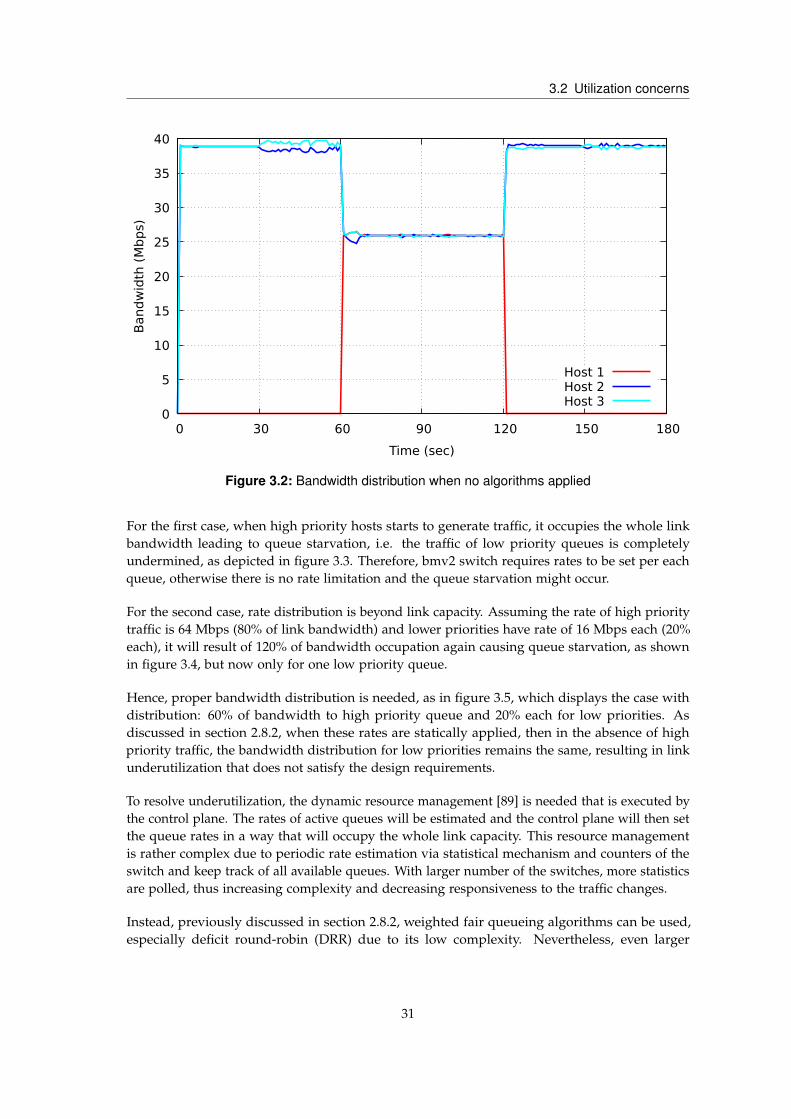
3.2 Utilization concerns
0
5
10
15
20
25
30
35
40
0 30 60 90 120 150 180
Band
wid
th (
Mb
ps)
Time (sec)
Host 1Host 2Host 3
Figure 3.2: Bandwidth distribution when no algorithms applied
For the first case, when high priority hosts starts to generate traffic, it occupies the whole linkbandwidth leading to queue starvation, i.e. the traffic of low priority queues is completelyundermined, as depicted in figure 3.3. Therefore, bmv2 switch requires rates to be set per eachqueue, otherwise there is no rate limitation and the queue starvation might occur.
For the second case, rate distribution is beyond link capacity. Assuming the rate of high prioritytraffic is 64 Mbps (80% of link bandwidth) and lower priorities have rate of 16 Mbps each (20%each), it will result of 120% of bandwidth occupation again causing queue starvation, as shownin figure 3.4, but now only for one low priority queue.
Hence, proper bandwidth distribution is needed, as in figure 3.5, which displays the case withdistribution: 60% of bandwidth to high priority queue and 20% each for low priorities. Asdiscussed in section 2.8.2, when these rates are statically applied, then in the absence of highpriority traffic, the bandwidth distribution for low priorities remains the same, resulting in linkunderutilization that does not satisfy the design requirements.
To resolve underutilization, the dynamic resource management [89] is needed that is executed bythe control plane. The rates of active queues will be estimated and the control plane will then setthe queue rates in a way that will occupy the whole link capacity. This resource managementis rather complex due to periodic rate estimation via statistical mechanism and counters of theswitch and keep track of all available queues. With larger number of the switches, more statisticsare polled, thus increasing complexity and decreasing responsiveness to the traffic changes.
Instead, previously discussed in section 2.8.2, weighted fair queueing algorithms can be used,especially deficit round-robin (DRR) due to its low complexity. Nevertheless, even larger
31

3 Proposed traffic management
0
10
20
30
40
50
60
70
80
0 30 60 90 120 150 180
Band
wid
th (
Mb
ps)
Time (sec)
Host 1Host 2Host 3
Figure 3.3: Queue starvation when no rates are set
0
10
20
30
40
50
60
70
0 30 60 90 120 150 180
Band
wid
th (
Mb
ps)
Time (sec)
Host 1Host 2Host 3
Figure 3.4: Queue starvation for improper bandwidth distribution
bandwidth allocation for high priority queue, DRR will not avoid round delays, as depicted infigure 3.6, increasing queueing delay.
32

3.2 Utilization concerns
0
5
10
15
20
25
30
35
40
45
50
0 30 60 90 120 150 180
Band
wid
th (
Mb
ps)
Time (sec)
Host 1Host 2Host 3
Figure 3.5: Static bandwidth distribution and link underutilization
Queue 0 High priority
Queue 1 Medium priority
DRR
Queue 2 Low priority
Queue 1 Round delay
Queue 2 Round delay
Figure 3.6: Round delays for high priority queue in DRR
Therefore, rate limited strict priority (RL-SP) needs to be applied to the high priority queue inorder to avoid delays, and combination of the queue scheduling algorithms (RL-SP DRR) needsto be designed in the following way: high priority traffic will be prioritized by providing largerbandwidth portion, only when it appears in the network. In this case, the remaining link capacity
33

3 Proposed traffic management
will be distributed among low priorities and scheduled in DRR fashion. Once high priority trafficleaves the network, the whole link capacity is again distributed and scheduled by DRR.
3.3 Traffic manager programmability
The current state of bmv2 switch does not allow to use south-bound API to program their trafficshaping mechanism, namely rate limited strict priority (RL-SP). Only a queue can be selectedwithin the scope of P4 program via metadata and a packet can then be emplaced to the queue.The queue scheduling is then applied based on the RL-SP. The scheduling can be configuredthrough the switch CLI, thus creating configuration vendor lock-in. To avoid this lock-in, fullyprogrammable configuration management needs to be provided.
In the source code of bmv2 [27], it can be observed that the current interface to traffic manager ishard-coded via metadata parsing and applying parsed priority number to the current packet.Hence, we can exploit the same approach by providing additional traffic management metadatathat will be parsed and provisioned to the traffic management achieving configuration withinthe scope of P4 program. As shown in figure 3.7, the switch will contain a table in the ingresspipeline that will provide traffic management configuration data to the P4 program, which willset metadata with these values. This table, as any data plane tables, can be modified throughcontrol plane via south-bound API. In this way, we can obtain programmable configuration oftraffic manager.
Metadata Parser
Traffic Manager
Traffic Management Metadata
Metadata
Ingress Table
P4 program
Traffic Management
ConfigurationData
Assign table datato metadata
Figure 3.7: Traffic management metadata provision to the traffic manager
3.4 Design discussion
It can be argued that this design avoids vendor lock-in, since a switch needs to support thesemetadata to provide such functionality. It is true, however, the purpose of P4 programminglanguage is to follow the abstraction that the switch architecture provides, which is independentfrom the vendor implementation. Therefore, it can be appealed that this design is architecturelock-in rather than vendor lock-in.
34

3.5 Traffic manager behavior
Next question can be asked of how appropriate and practical this design is. Currently no otherresearches have provided runtime programmability of traffic manager using P4 program andthis is the first attempt to implement it. This design is more of a concept rather than completesolution, since, firstly, the bmv2 switch is a reference software switch and is not meant for theproduction purposes, but for experimentations. Secondly, the performance of the designedalgorithm is far from ideal, because we try to emulate a hardware based (e.g. ASIC or FPGAbased) spatially parallel algorithm on the CPU-based sequential software switch. As will beexplained in the future work section, this should be extended and deployed on the programmablehardware (ASIC or FPGA) that provides spatial programmability.
Lastly, this design is stateless since most of the P4 constructs are stateless, meaning that everyinstruction in the program are independently applied to every packet [26]. Hence, each timewhen a packet arrives, the metadata will be parsed and provisioned to the traffic managerregardless of whether a configuration has changed or not. Therefore, again for the future work,an extern object (i.e. a stateful object in P4 terminology) needs to be provided to the switch thatwill apply traffic management configurations only when they are changed.
3.5 Traffic manager behavior
After defining requirements for the design of the traffic manager, explaining why P4 is preferredover OpenFlow and what challenges need to be resolved, we can formulate traffic managementfunctional behavior that later will serve as a basis for its implementation.
Traffic manager will:
1. use traffic shaping as a mechanism to regulate traffic flow in the shared Ethernet infrastructureto establish prioritized logical links;
2. use DRR as a fair queueing algorithm for non-prioritized traffic to fully utilize links and useRL-SP with only one queue for prioritized traffic;
3. be configurable via a metadata-based interface from within a P4 program.
4. use dedicated prioritized physical links, if this option is preferred;
35

3 Proposed traffic management
36

4 Implementation
This chapter provides implementation details of the traffic manager proposed in chapter 3.The architecture of bmv2 switch will firstly be explained in section 4.1, as well as the trafficmanagement engine currently implemented in the switch. The switch will be then extended tosupport rate limitation based on bytes per second units and deficit round-robin packet scheduling,as will be explained in section 4.2, and section 4.3 describes the metadata-based configuration ofthe traffic management.
4.1 bmv2 switch
bmv2 is a reference P4 software switch that allows to derive other software P4 targets. Inits repository [27], the examples of targets are given, e.g. simple_router, simple_switch, sim-ple_switch_grpc, psa_switch. For this work, we have considered simple_switch_grpc target due toits target-independent runtime configuration and refer it as a bmv2 switch from now on. Itis a wrapper of simple_switch target, so the changes of simple_switch functionality will lead tothe changes of simple_switch_grpc. Also targets derived from simple_switch are compatible withthe considered target, and we will utilize it to implement simple_switch targets with differentscheduling algorithms for future evaluation of algorithms. We have also considered experimen-tal version of simple_switch that needs to be compiled with enabling priority queue directive(SSWITCH_PRIORITY_QUEUEING_ON macros) in order to introduce strict priority scheduling.
The P4 constructs that are available for use as well as functional blocks are described in theswitch architecture file. Simple_switch_grpc target uses v1model, which will also be extended tosupport metadata for interfacing with traffic manager of the switch.
4.1.1 bmv2 architecture
bmv2 follows a protocol independent switch architecture, depicted in figure 4.1, which consistsof the following functional blocks: programmable parser, header representation, ingress andegress match+action pipelines, traffic management engine, deparser and additional metadata.When a packet enters a port of the switch, it is firstly processed by the parser, which is defined bya P4 program [26]. This is a state machine, which validates the packet header with the headersstack defined in the program. If the headers of the packet are invalid or have checksum collision,the packet can be dropped. For correct headers, the header representation is built out of headerfields and passed to the ingress match+action pipeline. Alongside, the metadata, which serve as

4 Implementation
the stateful objects between the pipeline stages, can be passed, although for the next packet thestate will be lost, since P4 constructs are designed to be stateless.
Eth IPv4
UDPTCP
RoCEv2iSCSI
Programmable Parser
HEADER REPRESENTATION
&& METADATA
Ingress Match+Action Traffic Manager Egress Match+Action DeparserPackets In
bmv2 Switch Architecture
Figure 4.1: Architecture of bmv2 switch
In the match+action pipeline, which can contain match+action tables populated by the controlplane, the fields of the header representation and metadata can be matched and certain actionsare performed, e.g. to modify the fields or metadata, upon the match. In case of a mismatch,either drop or no actions can be performed. The order, in which the pipeline tables are processed,is defined in the flow control block. Then the packet is enqueued within the queue engine of thetraffic manager. There, the packet scheduling can be applied before sending the packet to theegress match+action pipeline, which in turn, can further modify the header fields, e.g. IP headerchecksum computation. Eventually, the header representation is merged to the original packetand the packet is deparsed, i.e. sent to the output port of the switch.
4.1.2 bmv2 control plane
As briefly mentioned in the previous section, the pipeline tables are populated by the controlplane, which can be local (within the switch) or remote (outside the switch). Its workflow forthe interaction with the data plane is presented in figure 4.2. After the P4 program (switch.p4in the figure) is composed, it is compiled using target-specific compiler. In case of bmv2, it isp4c-bmv2-ss [98]. This compiler generates two artifacts, the behavior model of the target switch(switch.json file) and control plane API file (switch.p4info). The behavior model is then submittedto the switch process to be run (simple_switch_grpc process) and the defined behavior of theswitch is enabled, e.g. which tables to create and headers to parse. This driver also translatesthe messages sent by so-called P4Runtime server, which provides target independent interactionwith data plane and uses gRPC [99], remote procedure call (RPC) framework, as a programindependent transport.
The message format for such interaction is described with language and platform neutralserialization mechanism, Protobuf [100], and so is control plane API, which is submitted to theruntime server and control plane to describe the pipeline table structure and entries. Once the
38

4.1 bmv2 switch
bmv2 switch
switch.p4
P4 Compiler
Generate ControlPlane API
switch.json
switch.p4info
simple_switch_grpc
bmv2 Driver
P4Runtime Server (gRPC)
Remote Control Plane
Generate Switch Behavioral Model
Local Control Plane
p4runtime.protobuf
Figure 4.2: Local/Remote control planes and runtime configuration of the switch
API is established and the behavior and the structure of the switch are determined, the controlplane is now able to add, modify or delete the entries of pipeline tables.
4.1.3 bmv2 traffic management engine
bmv2 switch supports input and output first-in-first-out (FIFO) buffers shared for all ports andintermediate (egress) buffers for traffic management. The size of the buffers is packet-wise andas follows: input buffer – 1024, output buffer – 128, egress buffer – 64. This buffering process,shown in figure 4.3, is performed on the switch executional threads synchronized by the lockingmechanism. The device manager firstly sends available packets from the interfaces of the host,on which software switch resides, to the respective ports of the switch. The interface to portmapping is done, when the switch process is invoked with the passed parameters. For example,the command: simple_switch_grpc -i 1@iface1 -i 2@iface2 will map network interfaces ofthe system with the names iface1 and iface2 to the ports 1 and 2 of the switch, respectively.
Assuming that initially no packets are held in the buffers, the switch receives the first packetand enqueues it to the input buffer. Since the input buffer now contains the packet, the ingressthread is notified, and it dequeues the packet from the input buffer. Then, it parses packet headerrepresentation and metadata associated with the packet, classifies the packet based on themand enqueues to the corresponding multidimensional egress buffer with the rows of priorityqueues. Since, now egress buffer is not empty, one of the egress threads is invoked. The egressthread is selected based on the port-to-thread mapping. By default, it is done on the round-robinfashion with the number of threads equaling to the number of processor cores of the system. Forexample, for 2 cores system, there are 2 egress threads, and ports are mapped as follows: port 1to thread 1, port 2 to thread 2, port 3 to thread 1, port 4 to thread 2 and so on.
The egress buffers can have the packet scheduling ability. Once the egress thread is selected, itdequeues the packet from the egress buffer following the scheduling algorithm. Currently, bmv2
39

4 Implementation
packets in packets out
input ports output ports
input buffer output buffer
egress buffers (priority queues)
...
DeviceManager
IngressThread
EgressThreads
TransmitThread
Switch Receive
Send packet frominterface toport of the
switch
Enqueue to inputbuffer
Dequeue frominput buffer &
enqueue topriority queue
Dequeue frompriority queue
based onscehduling &enqueue to
output buffer
Dequeue fromoutput buffer &send to output
port
Figure 4.3: Ingress and egress ports and their threads pipeline models
supports rate limited strict priority scheduling. The departure time is calculated based on thequeue rate for each packet while being enqueued to the egress buffers. The rate has packets persecond (pps) units. The packets are then selected from the highest priority queue to the lowestwith the check of the departure time of the head packet of the queue, subsequently dequeuedfrom the egress buffer and enqueued to the output buffer, as shown in listing 4.1. Eventually, thetransmit thread empties the output buffer and sends the packet into the output port.
4.2 bmv2 extension stages
After introduction to bmv2 internals,the current state of bmv2 related to the traffic management,i.e. traffic shaping and queue management, is defined, as follows:
1. bmv2 supports N number of queues per egress port, where N is defined in the source code ofthe switch. By default, it is 8 queues per port;
2. the queues are scheduled using strict priority algorithm;
3. intrinsic_metadata.priority is used to select a priority queue;
4. rate limitation is based on packets per second (pps) units of measurement.
In order to follow the proposed design and behavior of the traffic manager, described in section3.5, certain extensions to the switch need to be made, namely, the units of rate measurement,packet scheduling algorithm and metadata-based programmability of the traffic manager. Hence,the following subsections will be dedicated to the implementation of these extensions.
40

4.2 bmv2 extension stages
/* Variables */int N // number of priority queuesqueue queues [0..N-1] // priority queues
/* Enqueue */function enqueue(queue , packet):
packet.departure_time = queue.last_sent + 1/queue.rate_pps
enqueue(queue , packet)
/* Dequeue */while (true):
selected_queue = NULL // the scheduled queuefor i = 0..N:
queue = queues[i]if queue is empty: continueif queue.head_packet.departure_time <= current_time:
selected_queue = queuebreak
if selected_queue is not NULL: dequeue(selected_queue)
Listing 4.1: Pseudo-code for strict priority packet scheduling in bmv2. Lock-based synchronizationis omitted for simplicity
4.2.1 Strict priority and rate limitation in bytes per second
When the rate limiting is performed using packets per second (pps) units, the packet size isassumed to be the size of the maximum transmission unit (MTU). Then, for packets which sizesare less than MTU or variable, the actual data rate distribution will be inaccurate. Therefore, it isproposed that the rate limiting will be in bytes per second (Bps) units of measurement, becausethe packet size is usually measured in bytes.
The queues of the egress port are based on a C++ priority queue data structure. It has thefollowing working principle: an object, which will be stored in the C++ priority queue, hasassociated priority. When it is emplaced into the queue, it will take the position such that allthe objects in the queue will be sorted according to their priority. The sorting is automaticallyapplied each time the new object is emplaced.
Hence, using priority queues we can perform rate limiting, as depicted in figure 4.4. We firstlycalculate the departure time of a packet (Di) based on the previous departure time (Di−1), thequeue rate (Ri) and the packet size (Pi):
Di = Di−1 +PiRi
41

4 Implementation
Then, we assign the departure time as a priority of the priority queue, emplace it and applysorting in the descendant order, i.e. earlies first. This way, we guarantee that the packets willbe ordered based on their departure time. The scheduler then polls the queues starting fromthe highest priority. It compares the head packet’s departure time of the queue with the "wall"clock whether it is time to send the packet to the output. If the time has not come, it polls nextqueue until one of the queues will not be served. If the departure time has been reached, thenthe scheduler dequeues a packet from the queue and starts again from the highest priority.
Calculate departure
time with R_0
High priority queue with rate R_0
P = 2000 @100
Dequeued packet
P = 400 @300
P = 700 @400
P = 700
Enqueued packet
P = 2000 @200
Wall clock: @160
Calculate departure
time with R_1
Low priority queue with rate R_1
P = 400 @300
P = 700 @450
P = 700
Enqueued packet
P = 2000 @150
Wall clock: @160
Go to low priority queue
P = 2000 @150
Dequeue packet
Figure 4.4: Rate limiting based on calculated departure time. P is a packet size in bytes
4.2.2 Rate limited strict priority with DRR
High priority queue
Medium priority queue
Low priority queue
DRR
Go to DRR, whensuspended
Output buffer
Rate limiter
Figure 4.5: Rate limited strict priority with DRR (RL-SP DRR)
After changing from packet rate to the data rate limitation for strict priority scheduling, we nowimplement deficit round-robin (DRR) as a fair queueing algorithm and combine these algorithmsin the way, depicted in figure 4.5: we reserve a high priority queue (HPQ) for strict prioritization,so that it will be always polled first, and lower priority queues (LPQs), e.g. medium and low
42

4.2 bmv2 extension stages
priorities, will be polled next. The HPQ occupies specific rate of a link and the remaining linkcapacity will be distributed among LPQ based on their DRR’s quantum values, as described insection 2.8.2.
RL-SP DRR algorithm
Listing 4.2 presents RL-SP DRR algorithm that is an extended version of original DRR algorithmof [28] to support RL-SP for HPQ.
/* Variables */int N // number of priority queuesqueue queues [0..N-1] // priority queuesactive_queue_list [0..N-1] // list of active queues
/* Enqueue */function enqueue(queue , packet):
if queue is HPQ:packet.departure_time = queue.last_sent + 1/queue.rate_Bps
else:packet.departure_time = current_timeif queue is empty:
active_queue_list.push(queue)
enqueue(queue , packet)
/* Dequeue */while (true):
selected_queue = NULL // the scheduled queueHPQ = queues [0]if queue is not empty and
queue.head_packet.departure_time <= current_time:selected_queue = HPQ
else:LPQ = DRR()selected_queue = LPQ
if selected_queue is not NULL: dequeue(selected_queue)
Listing 4.2: Pseudo-code for RL-SP DRR. Lock-based synchronization is omitted for simplicity
Firstly, a packet needs to be placed in the queue. Before placement, its departure time iscalculated. If HPQ is used, then the computation includes rate and packet size. For the LPQs, therate limitation is implicit and not based on the timing, but on quantum values, thus immediatedeparture time (current_time) is assigned. Also, to avoid queue misses when dequeueing fromLPQs is performed, the list of active LPQs (active_queue_list) is kept and updated, if therewere no packets in the LPQ before. The DRR is then performed with the active LPQs.
43

4 Implementation
The dequeueing is performed in two stages: it always polls HPQ first and if the departure timeof its head packet has not yet come, the algorithm then switches to LPQs and performs DRRto them, which is given in listing 4.3). The first (front) active queue is retrieved. If this queuewas not previously served, its deficit counter (DC) is incremented with the quantum value andcompared with the size of a head packet of the queue. If DC is less than the packet size, then thequeue is placed at the end of the active queues list and the round goes to the next active queueuntil one of the LPQs will not be served. If DC is sufficient, then the queue is selected and itshead packet is dequeued, preliminary decrementing packet size from the DC. After sending thepacket from the LPQ, the dequeueing again switches to the HPQ.
/* DRR algorithm */
int N // number of priority queuesqueue queues [0..N-1] // priority queuesactive_queue_list [0..N-1] // list of active queuesqueue last_served_queue = NULL;
function DRR():if active_queue_list is empty:
return NULL
queue = active_queue_list.front ()if queue not is last_served_queue:
increase queue.deficit_counter by queue.quantum
if queue.deficit_counter >= queue.head_packet.size:decrease queue.deficit_counter by queue.head_packet.sizelast_served_queue = queuereturn queue
else:active_queue_list.push_back(queue)return DRR()
Listing 4.3: Pseudo-code for DRR. Lock-based synchronization is omitted for simplicity
As mentioned in section 4.1.3, bmv2 has number of threads equal to the number of cores ofthe system and uses threads mapping for egress port selection in the round-robin fashion. Forimplementing DRR, it creates a problem since a thread will contain packets from different egressports in its queues, possibly causing collisions of queues configuration, e.g. the quantum valuesmight differ. Therefore, the same number of threads as the number of ports is used. Since defaultnumber of ports is 512, a switch process will yield 512 threads. For efficiency, the number ofthreads needs to be decreased. Therefore, 8 ports per switch are selected, because in the futureevaluation setup (section 6.4) switches with high number of ports will not be used. Each threadwill then process its set of the queues (1-to-1 thread-to-port mapping).
44

4.3 Metadata-based traffic management programmability
4.3 Metadata-based traffic management programmability
In order to allow P4 program to interact with traffic manager, additional intrinsic metadata areintroduced in the v1model and its source file is extended with:
• intrinsic_metadata.queue_rate – for setting the rate of the queue;
• intrinsic_metadata.queue_quantum – for setting quantum value of the queue.
The ingress thread parses metadata and puts the packet into the queue of the egress port basedon the parsed priority value in the metadata, as described in section 4.1. Additional metadata arealso parsed, and rate and quantum value are set for the specified queue. This way, we allow thetraffic manager to be configurable via P4 program running on the switch.
4.4 Implementation notes
It can be noted that while implementing and writing this work, the P4 community has imple-mented more features, modified current sources and fixed bugs of bmv2 switch and simpleswitch target. However, the queueing.h source file has not been modified in the main repositoryas of the end of this work, November 29, 2018 and the core of the queueing functionality wasimplemented in this file. The bmv2 version that is used for the extension is dated March 28, 2018.
45

4 Implementation
46

5 Validation and performance implications
5.1 Bandwidth distribution and CPU consumption
In order to validate the RL-SP DRR algorithm, the same experiment has been performed, as insection 3.2 with mininet network emulator and UDP traffic. The bandwidth allocation for highpriority traffic (Host 1) is 60% of link capacity; for medium (Host 2) and low (Host 3) priorities, itis 20% each.
Lower priorities (medium and low priorities) hosts have the same quantum values, thereforethey share bandwidth fairly. The result is depicted in figure 5.1. As it can be observed, the lowerpriorities hosts initially share the link bandwidth and their traffic is shaped. When high prioritytraffic appears, it is prioritized by allocating higher bandwidth share, whereas the remainingbandwidth is equally distributed between lower priorities, without explicitly specifying the queuerates. Thus, it can be said that the algorithm works and the link capacity is fully utilized.
0
5
10
15
20
25
30
35
40
45
50
0 30 60 90 120 150 180
Band
wid
th (
Mb
ps)
Time (sec)
Host 1Host 2Host 3
Figure 5.1: RL-SP DRR algorithm validation
However, its implementation is not efficient. It can be observed from the CPU utilization graphin figure 5.2 that RL-SP DRR (drr in the graph) needs more processing power than the cases

5 Validation and performance implications
when no algorithms applied (default in the graph) and strict priority (SP) only applied (strict inthe graph).
40
50
60
70
80
90
100
110
default strict drr
CPU
Uti
lizati
on (
%)
Algorithms
average (stddev)max
Figure 5.2: CPU utilization graph of the scheduling algorithms
5.2 Queue delays and buffers occupancy
Moreover, packet scheduling algorithms with explicit rate limitation cause queue delays. Todemonstrate this, an experiment with the same setup was performed, where the switch marks thepacket with calculated queue delay. In bmv2, specific intrinsic metadata named deq_timedeltais responsible for obtaining the queue delay.
In this experiment, only high priority host sends 100 UDP packets, each packet every second,with small payload (4 bytes) to remove the effect of transmission delay, and the server hostaccepts the packet and extracts the queue delay. The results of the delays are presented in figure5.3. The effect of the scheduling and rate limiting for high priority traffic is visible: the averagequeue delay for SP (69 µs) is higher compared to the case, when no scheduling is applied (59 µs).Since RL-SP DRR has higher processing time due to complexity, the average queue delay is thusthe highest for this experiment (97 µs).
Nevertheless, rate limitation is needed for traffic prioritization. For demonstration, the followingexperiment is performed. The high priority host sends UDP packets and the switch marks thepackets with queue delays, similarly to the previous experiment, while the lower priorities hostsare generating continuous UDP traffic with the rate of half of the link capacity in order to congestthe outgoing link. The queue delay measurements are shown in figure 5.4. When no schedulingis applied, the hosts share the same egress buffer. There is no prioritization for high priority
48

5.2 Queue delays and buffers occupancy
0
100
200
300
400
500
600
def strict drr
Queue d
ela
y (
µs)
Algorithms
average (stddev)max
Figure 5.3: Queue delay for different algorithms when only high priority traffic is generated
0
1000
2000
3000
4000
5000
6000
7000
8000
9000
def strict drr
Queue d
ela
y (
µs)
Algorithms
average (stddev)max
Figure 5.4: Queue delay of high priority host for different algorithms when all the hosts generateUDP traffic
traffic and its packets are delayed by 5167 µs on average. For SP the delay is the lowest, 42.35µs on average, whereas for RL-SP DRR, the average queue delay is relatively high, 2717 µs on
49

5 Validation and performance implications
average, but lower than the case without scheduling. To explain high queue delay of RL-SPDRR of this experiment, the buffers occupancy needs to be examined and compared to the SPscheduling.
The same experiment is repeated, but now the high priority packets are marked with the numberof packet buffered in the input, egress and output buffers. The queue model for this experimentis presented in figure 5.5. Three hosts are generating traffic with arrival rate λ and the forth hostis receiving at the link rate, or service rate µ, which is split into the service rate of the queues(µ1−3). The arrival rates for this experiment are:
For high priority (46 bytes UDP/IP/Ethernet headers + 4 bytes payload): λ1 = 400bits/s µ
For medium priority: λ2 = 0.5µ
For low priority: λ3 = 0.5µ
When considering SP scheduling, the explicit queue rates distribution is then:
60% of link capacity for high priority: µ1 = 0.6µ
20% of link capacity for medium priority: µ2 = 0.2µ
20% of link capacity for low priority: µ3 = 0.2µ
Therefore, the total sum of lower priorities queue rates (0.4µ < µ) underutilize the output bufferand the buffer is free for high priority packets. The lower priorities egress buffers and inputbuffer, on the other hand, are overutilized (e.g. λ2 = 0.5µ > 0.2µ).
input buffer output buffer
λ2
egress buffers
λ1
λ3
µ2
µ1
µ3
µ
1024
64 x3
128
> High priority > Medium priority > Low priorityλ > arrival rateµ > service rate
Figure 5.5: Queue model for the experiment with 4 hosts. Three hosts are generating the trafficto the forth host. Input and output buffers have a size of 1024 and 128 packets,respectively, whereas each buffer of three egress buffers has the size of 64 packets
For RL-SP DRR, the rate distribution for lower priorities queues is implicit. Since no delays areassumed for these queues, unlike for SP, the link rate (µ) should be used and for each low priorityqueue, it is half of link rate due to fair share. Therefore, the rate distribution is following:
For high priority: µ1 = 0.6µ
For medium priority: µ2 = 0.5µ
For low priority: µ3 = 0.5µ
50

5.2 Queue delays and buffers occupancy
This distribution, in turn, overruns output buffer (µ2 + µ3 = µ), causing the delay for highpriority packets. However, the egress buffers are occupied less, because arrival rates are sustainedwith service rates of the egress buffers (e.g. λ2 = 0.5µ = µ2).
The obtained results, shown in figure 5.6, confirm the analysis of buffer occupancies. The egressbuffers are occupied completely for SP, due to the large difference in arrival and service rates.However, this does not allow the output buffer to be full, thus giving virtually no delays for highpriority packets. The egress buffers are occupied less for RL-SP DRR, however, due to implicitrate distribution based on quantum values and output buffer share, the output buffer is overrunby low priorities. The input buffer for both SP and RL-SP DRR was not considerably occupied.
0
20
40
60
80
100
120
140
input egress output
Buff
er
size
(num
ber
of
pack
ets
)
Buffers
DRR STRICT
Figure 5.6: Input, egress and output buffers occupancy for strict priority and RL-SP DRR
51

5 Validation and performance implications
52

6 Evaluation setup
This chapter presents evaluation setup and model for the implemented traffic management. Theenvironment and tools used for obtaining evaluation metrics are described in section 6.1. Section6.2 describes different test cases that demonstrate the behavior of the traffic management, namelywhen the traffic management is set at the runtime, when the traffic management is set proactivelyand how the traffic management handles MPI communication. The test cases will compare theimplemented traffic management with best-effort approach and strict priority scheduling. Theevaluation model as well as how the experiments are performed for each test case are explainedin section 6.3. And section 6.4 presents the topologies used to emulate different traffic patterns inthe cloud infrastructure.
6.1 Setup and tools
6.1.1 Mininet
To deploy the evaluation setup we used network emulator, mininet [101], running on the physicalhost with 4 cores of Intel i5-4590 and 16 GB of memory. Mininet allows to programmaticallyemulate and deploy virtual networks and create virtual hosts and switches that are separated byprocess-based virtualization and connected using virtual Ethernet pairs (veth).
The hosts are represented as multiple emulated physical machines sharing same functionalityas the machine, on which mininet is deployed. They can be accessed via Mininet CLI or APIto perform shell commands. The switches connect the hosts, and the link parameters, such asbandwidth or link delay, are configurable. By default, the switches have support of OpenFlowand can be configured via control plane (either OpenFlow controller or switch CLI).
To support P4, the mininet switch needs to be extended and assigned to the bmv2 process. Afterthe creation of veth interfaces for the mininet switch, the bmv2 switch associates its ports withthe veth interfaces same way as it associates the ports with any interfaces. Thus, the traffic flowis intercepted by the bmv2 switch. To enable this in our setup, the code from the P4 tutorials wasused [102] as the basis for P4-enabled network in mininet, and was modified to create customevaluation scenarios.

6 Evaluation setup
6.1.2 iperf
For measurements of network metrics, iperf tool was used. It involves an iperf client andan iperf server that establish TCP or UDP based communication, exchange the data withvarious transfer rates and data sizes and calculate the end-to-end metrics. With newer versionof iperf (iperf 2.8), it allows to measure basic metrics: TCP/UDP bandwidth (or throughput),number of retransmissions, jitter and packet losses, as well as enhanced time metrics: round-triptime (RTT) and one-way latency. It provides formatting with machine-readable format, e.g.comma-separated values (CSV), only for basic metrics. To support formatting of time metrics,the source code of iperf was extended.
6.1.3 MPICH
MPICH 3.2 [30] is chosen as an MPI implementation due to its portability and ease to install andconfigure. The hosts that will be exploited for an MPI application are defined in the hosts file(hosts-file) in the form of a list of their hostnames and passed to the mpirun process. As anexample, for two hosts employed to run the MPI application (mpi_application):
IP address to hostname mapping is in the configuration file /etc/hosts:10.0.1.1 host-110.0.1.2 host-2
List of the hosts participating in MPI process is in hosts-file:host-1host-2
Command to run MPI application over these hosts:mpirun -n 2 -f hosts-file ./mpi_application
The communicator uses secure shell (SSH) protocol to access the hosts, thus the hosts in mininetneed to enable their sshd server processes. As a consequence, the servers need to generate SSHkey pairs (public and private) in order to give permission to access.
For efficiency, MPICH allocates running processes into the individual CPU cores of the system.Thus, when specifying 2 processes within a single physical host, as in the case with mininetemulation, 2 CPU cores will be utilized. In the 4 core setup (400% CPU) used in this work,200% CPU is allocated during the execution of an MPI application and the remaining for otherprocesses, such as bmv2 switch processes.
54

6.2 Test cases
6.2 Test cases
What has been implemented and validated so far is the traffic manager on bmv2 switch, runningRL-SP DRR scheduling algorithm and metadata-based configuration. What can be demonstratedin this scope is how the switch handles:
1. traffic prioritization by observing higher bandwidth distribution and fewer packet losses;
2. link utilization without additional bandwidth calculations, i.e. proactive configuration;
3. programmability of the traffic manager via P4 pipeline table.
For these, we composed three evaluation test cases, RUNTIME, PROACTIVE, MPI, and for eachtest case, the comparison between RL-SP DRR scheduling algorithm, strict priority and best-effortapproach will be presented. The test cases are:
1. RUNTIME – RUNTIME CONFIGURATION to PRIORITIZE CURRENT TRAFFIC FLOW:this test case is depicted in figure 6.1. The hosts are generating traffic with no prioritizationapplied. The links are fully utilized. After 90 seconds, the prioritization phase is enabled for highpriority traffic for another 90 seconds. It is then disabled again. The time until the prioritizationis established and the behavior of the traffic can be observed in this scenario.
0 Time (sec)90 180 270
33%
33%
33%
20%
20%
60%
33%
33%
33%
Start experiment No prioritization
Full link capacity
Enable prioritization Disable prioritization End experiment
→ High priority → Medium priority → Low priority
Figure 6.1: RUNTIME test case
2. PROACTIVE – PROACTIVE CONFIGURATION and HIGH PRIORITY TRAFFIC INJEC-TION: this test case is depicted in figure 6.2. Prioritization is configured, so that the links arefully utilized, and only low priority hosts are generating the traffic. After 90 seconds, the highpriority traffic appears for 90 seconds. The link utilization and traffic behavior can be observedfor this scenario, as well as how the configuration of the link is performed.
3. MPI – PROACTIVE CONFIGURATION and MPI PING-PONG LATENCY MEASURE-MENT: this test case is depicted in figure 6.3. Prioritization is configured, so that the links arefully utilized. Low priority hosts are generating the traffic and high priority hosts are running an
55

6 Evaluation setup
0 Time (sec)90 180 270
50%
50%
20%
20%
60%
Start experiment With prioritization
Full link capacity
High priority appears High priority leaves End experiment
→ High priority → Medium priority → Low priority
50%
50%
Figure 6.2: PROACTIVE test case
MPI application that measures ping-pong latency by sending messages with different sizes and100 times per size. The experiment is complete as soon as the MPI measurements are over.
0 Time (sec) N
Full link capacity
End experiment MPI end
→ High priority → Medium priority → Low priority
Start experiment With prioritization
MPI start
20%
20%
60%
Figure 6.3: MPI test case
The scheduling algorithms are implemented as separate P4 targets and the naming conventionfor the scheduling algorithms and their role are defined as follows:
1. NO-ALG: No scheduling, best-effort approach, out-of-box default bmv2 switches.
2. STRICT-ALG – STRICT PRIORITY: Strict priority is enabled on the switches. The ratelimitation is applied by following the bandwidth allocation for each type of traffic, thus shapingthe traffic.
3. DRR-ALG – RATE-LIMITED STRICT PRIORITY WITH DEFICIT ROUND-ROBIN: RL-SP DRR is enabled on the switches. High priority traffic will have same rate limitation as inthe strict priority, but the other types of traffic will have bandwidth distribution based on theirquantum values. The traffic is also shaped.
56

6.3 Evaluation model
Since we use wrapper target, simple_switch_grpc, which allows to change base target only at thecompile time, we cannot produce simultaneous algorithms. Hence, for each algorithm, the targetis recompiled and the evaluation is performed separately.
These test cases have been specifically designed to see the benefits of using DRR-ALG overNO-ALG and STRICT-ALG in terms of latency, utilization of available bandwidth and scalability.It will be shown that their behavior is similar when utilizing the links fully, however, the wayit is achieved differs. The test cases will be then deployed on multiple emulated topologiesthat demonstrate the communication of virtual machines in the virtual access tier (within aphysical host), in the access tier (across a top-of-rack switch) and in the aggregation tier (acrossan aggregation switch).
6.3 Evaluation model
Metrics and test procedure
The participating hosts will be divided into 3 groups, representing 3 services: high, medium andlow priority services, and occupy respective queues when scheduling is applied. The bandwidthdistribution of the prioritization scheme will be set as: 60% of the link capacity for high priority,20% for medium and 20% for low priority, so that for congested outgoing link of the virtualswitch, this distribution will be applied. The condition that the links must be fully utilized forany test case is also assumed.
For the measurements, TCP will be considered as an emulation of MPI traffic and UDP asRoCEv2 traffic. The iperf clients will generate respective traffic and iperf servers will calculatesome of the performance metrics, described in QoS standards for IP-based networks [103]:
• Bandwidth distribution metrics:
– TCP bandwidth, as the throughput dependent on packet losses
– UDP bandwidth, as the throughput not dependent on latency and losses
• UDP percentage of packet losses
• UDP average one-way latency
The focus of the experiments will be on obtaining bandwidth, packet losses and one-way latency.
The default connection type for iperf is TCP and default congestion control is CUBIC [104], thusby running on the server host:
iperf -s
iperf server will be listening for TCP connections. The UDP iperf server requires explicit flag tobe set:
57
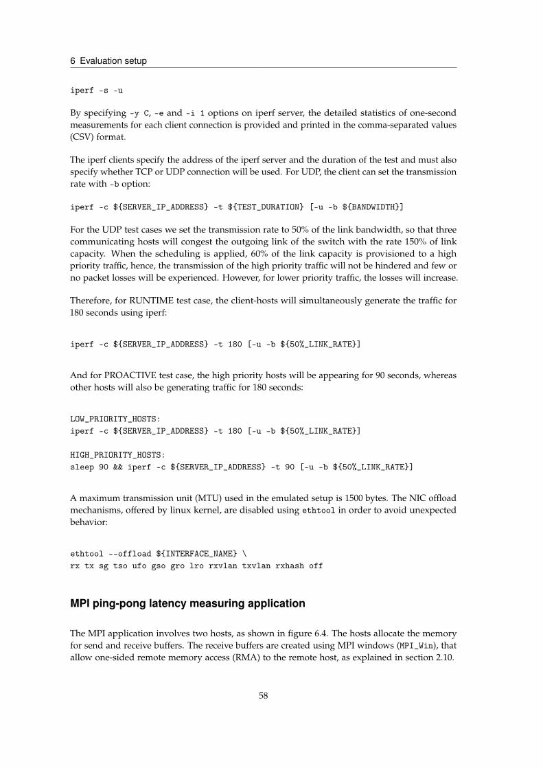
6 Evaluation setup
iperf -s -u
By specifying -y C, -e and -i 1 options on iperf server, the detailed statistics of one-secondmeasurements for each client connection is provided and printed in the comma-separated values(CSV) format.
The iperf clients specify the address of the iperf server and the duration of the test and must alsospecify whether TCP or UDP connection will be used. For UDP, the client can set the transmissionrate with -b option:
iperf -c $SERVER_IP_ADDRESS -t $TEST_DURATION [-u -b $BANDWIDTH]
For the UDP test cases we set the transmission rate to 50% of the link bandwidth, so that threecommunicating hosts will congest the outgoing link of the switch with the rate 150% of linkcapacity. When the scheduling is applied, 60% of the link capacity is provisioned to a highpriority traffic, hence, the transmission of the high priority traffic will not be hindered and few orno packet losses will be experienced. However, for lower priority traffic, the losses will increase.
Therefore, for RUNTIME test case, the client-hosts will simultaneously generate the traffic for180 seconds using iperf:
iperf -c $SERVER_IP_ADDRESS -t 180 [-u -b $50%_LINK_RATE]
And for PROACTIVE test case, the high priority hosts will be appearing for 90 seconds, whereasother hosts will also be generating traffic for 180 seconds:
LOW_PRIORITY_HOSTS:iperf -c $SERVER_IP_ADDRESS -t 180 [-u -b $50%_LINK_RATE]
HIGH_PRIORITY_HOSTS:sleep 90 && iperf -c $SERVER_IP_ADDRESS -t 90 [-u -b $50%_LINK_RATE]
A maximum transmission unit (MTU) used in the emulated setup is 1500 bytes. The NIC offloadmechanisms, offered by linux kernel, are disabled using ethtool in order to avoid unexpectedbehavior:
ethtool --offload $INTERFACE_NAME \rx tx sg tso ufo gso gro lro rxvlan txvlan rxhash off
MPI ping-pong latency measuring application
The MPI application involves two hosts, as shown in figure 6.4. The hosts allocate the memoryfor send and receive buffers. The receive buffers are created using MPI windows (MPI_Win), thatallow one-sided remote memory access (RMA) to the remote host, as explained in section 2.10.
58

6.3 Evaluation model
The first host, with rank 0, sends messages of various sizes from its send buffer to the receivebuffer (MPI_Win) of the second host, with rank 1, using MPI_PUT function, while registering thesending time (t1) with MPI_Wtime function. Once the second host receives the message, it sendsit back to the first host following the same way. Upon receiving the message from the secondhost, the receive time (t2) is registered. Therefore, ping-pong latency is the difference betweenreceive and send times (t2 − t1). The source code of [105] is used for these measurements.
H2H1
MPI_Win MPI_Win
MPI_PUT
TCP/IP
t_1
t_2
MPI_PUT
MPI_Wtime
Send buffer Send buffer
Rank 0 Rank 1
Figure 6.4: MPI ping-pong latency measuring application using MPI_PUT and MPI_Wtime
P4 switch for evaluation setup
The switches will be running the same P4 program that defines two pipeline tables, as shown infigure 6.5. The first table (src_ip_prio) provides priority queue, queue rate and queue quantumbased on the source IP address of the packet. Upon the table match, the program sets respectivemetadata via set_priority action. There are 8 priority queues in the switch (section 4.2.2). Thequeue 7 is reserved for high priority traffic, other queues 0-6 for low priorities. The second table(ipv4_lpm) determines outgoing port based on destination IP address and sets destination MACaddress of the frame through ipv4_forward action. The IP matches of the tables have long prefixmatch (LPM), so that the forwarding based on network address is performed. The source code ofthe switch and how it can be compiled are presented in appendix 1.
Each switch has a configuration file (runtime.json) with the data for the tables. The control plane,running locally, populates initially the tables from the file upon deploying the setup to establishrouting paths and mapping of source IP address to the priority queues. The initial schedulingparameters, rate and quantum, are also loaded from the file. The src_ip_prio table is thenmodified via control plane commands, which has the following format:
table_modify src_ip_prio set_priority $ENTRY_ID $PRIORITY $RATE $QUANTUM
59

6 Evaluation setup
P4 switch
ipv4_lpm:
dst_IP → forward → (out_port, dst_MAC)
metadata.egress_spec = out_port; ethernet.dstAddr = dst_MAC;
src_ip_prio:
src_IP → set_priority → (prio, rate, quantum)
metadata.priority = prio;metadata.queue_rate = rate;metadata.queue_quantum = quantum;
Figure 6.5: Pipeline tables of P4 switch used in evaluation. Left table sets priority parametersbased on source IP. Right table sets forwarding rules
For convenience, the pair of (ENTRY_ID, PRIORITY) of the high priority is (0, 7) or (0, 6), if theprioritization is disabled, for medium priority is (1, 5) and for low is (2, 4).
It could be noted that for NO-ALG and STRICT-ALG priorities not all the parameters arenecessary, e.g. NO-ALG has no scheduling and STRICT-ALG does not need quantum. For them,these parameters take no effect on the traffic manager, since the parsing of standard_metadata foreach target is different and includes metadata specific to the algorithm.
Control plane behavior for RUNTIME test case
In RUNTIME test case, initially all hosts have no prioritization, thus the bandwidth should bedistributed fairly. For three types of services, 33% will be allocated per service and specifiedin the configuration file. After 90 seconds, the prioritization is enabled. For NO-ALG, only theforwarding table needs to be populated and thus, no control plane actions afterwards are appliedfor prioritization during the experiment.
For STRICT-ALG, in order to utilize the links fully, the bandwidth distribution is precalculatedfor simplicity and applied at the exact moment, when prioritization needs to be enabled anddisabled. Since there will be three entries that need modifications, three control plane commandswill be sent to the data plane each time the prioritization changes. For STRICT-ALG, the queue 6can be used, because high priority just has higher queue number than lower priorities, thus thecommands to enable prioritization are:
table_modify src_ip_prio set_priority 0 6 $60%_LINK_RATE $QUANTUMtable_modify src_ip_prio set_priority 1 5 $20%_LINK_RATE $QUANTUMtable_modify src_ip_prio set_priority 2 4 $20%_LINK_RATE $QUANTUM
And to disable prioritization and enable fair share:
table_modify src_ip_prio set_priority 0 6 $33%_LINK_RATE $QUANTUM
60

6.3 Evaluation model
table_modify src_ip_prio set_priority 1 5 $33%_LINK_RATE $QUANTUMtable_modify src_ip_prio set_priority 2 4 $33%_LINK_RATE $QUANTUM
For DRR-ALG, to enable initial fair share, low priority queues and same quantum values willbe set to 7000 in the file. For prioritization, the queue will be changed to high priority queue 7and the rate will be specified. The remaining of the link rate is fairly distributed between lowerpriorities:
table_modify src_ip_prio set_priority 0 7 $60%_LINK_RATE $QUANTUM
And to disable prioritization, the queue 6 will be selected back:
table_modify src_ip_prio set_priority 0 6 $RATE $QUANTUM
Control plane behavior for PROACTIVE test case
In this test case, the configuration of prioritization scheme is predefined. However, since highpriority traffic will appear only after the 90 seconds of the experiment, the links will not beutilized for STRICT-ALG. Thus, proactive approach is not possible without explicit rate settingswhen high priority traffic appears. Thus, similarly to RUNTIME test case, the rates will bespecified, but only for lower priorities. To enable prioritization:
table_modify src_ip_prio set_priority 1 5 $20%_LINK_RATE $QUANTUMtable_modify src_ip_prio set_priority 2 4 $20%_LINK_RATE $QUANTUM
And to have fair share between only two services after the high priority traffic stops generatingtraffic:
table_modify src_ip_prio set_priority 1 5 $50%_LINK_RATE $QUANTUMtable_modify src_ip_prio set_priority 2 4 $50%_LINK_RATE $QUANTUM
For NO-ALG and DRR-ALG, the proactivity is possible. After initial configuration with pri-oritization scheme, the links will be utilized, because NO-ALG is best-effort and DRR-ALG isweighted fair queueing algorithm.
Control plane behavior for MPI test case
The same way, as for the PROACTIVE test case, the prioritization is enable beforehand. However,after the start of the experiment, no control plane intervention is needed.
61

6 Evaluation setup
6.4 Emulated topologies
Assumptions
In mininet environment, the hosts are virtualized and considered as physical machines. Since thecloud infrastructure needs to be emulated, the hosts will be considered as virtual machines andthe access switches for them, as virtual switches. Thus multiple hosts connected to the accessswitches will embody physical host and uplink of the virtual access switch will be physicalinterface connected to the access switch, as depicted in figure 6.6.
VM2 VM3 VM4VM1
vSwitch
Physical host
H2 H3 H4H1
Mininet switch
Mininet environmentReal setup
Access switch Mininet switch
Mininet hosts
Figure 6.6: Mininet setup represents real setup in cloud infrastructure
For simplicity, the network of the tenants will not be separated and they will share samebroadcasting domain. No network virtualization, e.g. VxLAN will be applied. The hosts willhave /32 prefix in their IP addresses, therefore, no ARP requests will be produced and thedestination MAC address in the sending frames is thus the broadcast MAC address. The virtualaccess switches will then set destination MAC addresses of respective destination host and routethem by their IP addresses. Thereby, the hosts will explicitly be connecting to each other usingLayer 3 addressing and an IP address of a host can be determined as follows:
10.0.$SWITCH_ID.$HOST_ID
where $SWITCH_ID and $HOST_ID can be obtained from the topology elements labeling. Forexample, Host 4 (H4) connected to the Switch 2 (S2) will have an IP address: 10.0.2.4.
As discussed in section 2.8, the traffic management is performed at the edge of the network, thusvirtual access switches will have packet scheduling enabled, and physical access and aggregationswitches will be just forwarding traffic to the destined ports. Core tier will not be included,because introducing another tier will only increase setup complexity and CPU consumption,which will affect the traffic management performance. Multipath interconnection and physical
62

6.4 Emulated topologies
links prioritization will also be omitted, since the test scenarios focus on the behavior of trafficmanager of the switches, rather than on resiliency.
Although typical HPC applications deployment requires lossless interconnect, and the priorityflow control can be in Ethernet infrastructure via IEEE 802.1p extension, mininet does not supportsuch extension. Hence, we consider our setup lossy and traffic management can decrease thepacket losses to a certain extend, but not eliminate them to the bare minimum.
6.4.1 TOPO-1: Topology-1, star
The star topology will simulate the case, when communication of VMs is within a physical host,i.e. in virtual access tier, and one VM is used to house multiple services. Figure 6.7 depicts asimple star topology with 4 hosts. Hosts are generating TCP and UDP traffic using iperf. Host4 (H4) is an iperf-server and Hosts 1, 2, 3 are iperf-clients that are connecting to H4. It can beseen that the link between the virtual switch (S1) and H4 will be congested, thus for this link theprioritization scheme will be applied as priorly discussed. Host 1 (H1) is a high priority hostand 60% of this link capacity will be allocated for it. Medium (H2) and low (H3) priorities hostswill have 20% of overall bandwidth each. For MPI test case, H1 and H4 are running the MPIping-pong latency measuring application.
The entries for the forwarding table (ipv4_lpm) and priority mapping table (src_ip_prio) of theswitch S1 are described in details in appendix 2, tables 2.1 and 2.2.
H → High priority → Medium priorityH → Low priorityH
H2 H3 H4H1
iperf -siperf -ciperf -ciperf -c
1S1
2 3 4
iperf connections
H1 → H4
H2 → H4
H3 → H4
60%
20% 20%
H → Client → ServerH
vSwitch
Physical host
* *
→ MPI hostH*
Figure 6.7: Simple star with 4 hosts. Hosts H1, H2 and H3 are iperf-clients and host H4 is aniperf-server. Link between H4 and the switch S1 is congested and packet schedulingis applied to it for prioritization
63

6 Evaluation setup
Performance consideration for link capacity selection
Mininet allows to set a bandwidth for each link in the emulated topology. With the increase ofbandwidth, the CPU utilization also increases. The number of switches also affects the CPUutilization. There is an obvious dependency: when the traffic injection rate is higher, the switchesneed to process more packets and thus their CPU consumption is higher. Therefore, the linkbandwidth should be selected properly. As was stated in section 5.1, the DRR-ALG consumesmore CPU than the other cases. Thus, the CPU utilization of this algorithm will serve as a upperbound for link selection.
For simplicity, the prioritization is enabled and the traffic from the hosts are generated simultane-ously. The following figures 6.8a and 6.8b show the average and maximum CPU utilization forTCP and UDP connections over the different bandwidth values.
From the graphs, it can be seen that CPU utilization increases as the bandwidth is increased.The overall consumption of CPU for TCP is higher throughout all bandwidth values comparedto UDP, and CPU saturation can be observed for TCP case at 550 Mbps (210%) and for UDP -at 700 Mbps (175%). This is because the acknowledgments from the servers to the clients arealso generating traffic in the opposite direction involving output ports of the clients, and hencemore threads, to be processed, whereas UDP communication is one-directional. Also, the TCPcongestion control creates computation overhead affecting the CPU consumption. Additionally,it affects the bandwidth distribution, since it reacts to the packet losses via retransmissions,dropping TCP window size.
The number of retransmissions for high priority traffic, as depicted in figure 6.9a, increaseswith the increase of bandwidth, since the buffers of the switch (section 4.1.3) overrun faster andpossibility of packet loss is higher. Starting from 200 Mbps the best-effort bandwidth distribution(figure 6.9b) is formed. For UDP case, the bandwidth converges at 650 Mbps, shown in figure6.9c, because bmv2 switch with DRR-ALG is CPU bounded and it is within CPU saturationregion.
Therefore, the upper bound for TCP is 150 Mbps and for UDP is 600 Mbps and the 100 Mbps linkwill be used for this topology with one switch, which will have 77% of average CPU consumptionfor TCP connectivities and 66% of CPU for UDP. For the topologies with more switches, firstly,the links with 100 Mbps will be used and the same experiment will be executed. If best-effortbandwidth distribution is observed for TCP connectivity, when DRR-ALG prioritization isapplied, the link capacity will be dropped, until the clear prioritization behavior will be observed.This is done in order to compare different algorithms in a fair manner.
6.4.2 TOPO-2: Topology-2, tree (depth=1)
The tree topology with the depth of 1 will simulate communication of VMs within an access tieror across a top-of-rack (ToR) switch. Figure 6.10 shows such topology. Each VM connects only toone VM on the adjacent leaf. The first leaf represents iperf-clients and the second leaf representsiperf-servers. The links between physical hosts and the ToR switch will thus be congested andfor these links mentioned prioritization scheme will be applied by the virtual switches. Hosts
64

6.4 Emulated topologies
0
50
100
150
200
250
300
50 100 150 200 250 300 350 400 450 500 550 600 650 700 750 800 850 900 950 1000
CPU
Uti
lizati
on (
%)
Bandwidth (Mbps)
average (stddev)max
(a) CPU vs bandwidth for TCP connections
0
50
100
150
200
250
300
50 100 150 200 250 300 350 400 450 500 550 600 650 700 750 800 850 900 950 1000
CPU
Uti
lizati
on (
%)
Bandwidth (Mbps)
average (stddev)max
(b) CPU vs bandwidth for UDP connections
Figure 6.8: TOPO-1: CPU vs bandwidth
H1 and H4 are high priority hosts. Hosts H2, H5 are medium priority and H3, H6 are lowpriority hosts. For MPI test case, H1 and H4 are running the MPI ping-pong latency measuring
65

6 Evaluation setup
0
50
100
150
200
250
300
50 100 150 200 250 300 350 400 450 500 550 600 650 700 750 800 850 900 950 1000
Num
ber
of
retr
ansm
issi
ons
Bandwidth (Mbps)
average (stddev)max
(a) Number of retransmissions vs bandwidth for TCP connections
0
10
20
30
40
50
60
70
0 5 10 15 20 25 30 35 40 45
Bandw
idth
(M
bps)
Time (sec)
Host 1Host 2Host 3
(b) Best-effort bandwidth distribution at 200 Mbps linkcapacity for TCP connections
0
50
100
150
200
250
0 5 10 15 20 25 30 35 40 45
Bandw
idth
(M
bps)
Time (sec)
Host 1Host 2Host 3
(c) Best-effort bandwidth distribution at 650 Mbps linkcapacity for UDP connections
Figure 6.9: TOPO-1: Number of retransmissions vs bandwidth. Best-effort bandwidth distributionwith high link capacities
application. The entries for the forwarding and priority mapping tables also can be found inappendix 2, tables 2.3 and 2.4.
Performance consideration for link capacity selection
In the TOPO-1 performance consideration, it was stated, that initially the 100 Mbps links willbe selected and TCP traffic will be generated simultaneously with enabled prioritization andDRR-ALG.
66

6.4 Emulated topologies
H → High priority → Medium priorityH → Low priorityH
H2 H3H1
iperf -ciperf -ciperf -c
H5 H6H4
iperf -siperf -siperf -s
S11 2 3
41S2
2 34
S31 2
60%
20% 20%
iperf connections
H1 → H4
H2 → H5
H3 → H6
H → Client → ServerH
vSwitch vSwitch
Physical host Physical host
ToR
* *
→ MPI hostH*
Figure 6.10: Tree (depth=1) with 6 hosts. Hosts H1-H3 are iperf-clients and hosts H4-H6 areiperf-servers. Links between physical hosts and ToR switch are congested andpacket scheduling is applied to them for prioritization
For 100 Mbps, the best-effort distribution was observed, as depicted in figure 6.11a, signifyingthat the link capacity should be dropped. After dropping the link capacity to the 50 Mbps, theprioritization is now visible, as depicted in figure 6.11b. Thus the link capacity for this topologyis 50 Mbps.
0
10
20
30
40
50
60
0 30 60 90
TCP B
andw
idth
(M
bps)
Time (sec)
Host 1Host 2Host 3
(a) Best-effort bandwidth distribution with 100 Mbpslink capacity for TCP connections
0
5
10
15
20
25
30
0 30 60 90
TCP B
andw
idth
(M
bps)
Time (sec)
Host 1Host 2Host 3
(b) Prioritized bandwidth distribution with 50 Mbpslink capacity for TCP connections
Figure 6.11: TOPO-2: link capacity selection based on bandwidth distribution
67

6 Evaluation setup
6.4.3 TOPO-3: Topology-3, tree (depth=2)
The tree topology with the depth of 2 will simulate communication of VMs within an aggregationtier or across an aggregation switch as depicted in figure 6.12. There, the branches from theaggregation switch are separated into the iperf-clients (left branch) and the iperf-servers (rightbranch) VMs. For MPI test case, H1 and H4 are running the MPI ping-pong latency measuringapplication. The links between physical hosts and ToR switches will again be congested and thistime, the links between ToR switches and the aggregation switch will also be congested. Sincethe later source of congestion is related to the oversubscription problem at the aggregation tier,the capacity of these links will be doubled to sustain the load of two connected ToR switches.The prioritization scheme will then be applied by the virtual switches. The entries for the tablescan be found in appendix 2, tables 2.5, 2.6 and 2.7.
H → High priority → Medium priorityH → Low priorityH
H2 H3H1
iperf -ciperf -ciperf -c
H5 H6H4
iperf -siperf -siperf -s
S11 2 3
41S2
2 34
S51 2
H8 H9H7 H11 H12H10
iperf -siperf -siperf -s
S31 2 3
41S4
2 34
S61 2
3 3
iperf -ciperf -ciperf -c
60%
20% 20%
iperf connections
H1 → H7
H2 → H8
H3 → H9
iperf connections
H4 → H10
H5 → H11
H6 → H12
S71 2
H → Client → ServerH
Physical host Physical host Physical host Physical host
vSwitch vSwitch vSwitch vSwitch
ToR ToR
Aggregation
**
→ MPI hostH*
Figure 6.12: Tree (depth=2) with 12 hosts. Hosts H1-H6 are iperf-clients and hosts H7-H12 areiperf-servers. Links between physical hosts and ToR switch are congested andpacket scheduling is applied to them for prioritization. The capacity of the linksbetween ToR and aggregation is doubled
Performance consideration for link capacity selection
Similarly to link selection for TOPO-2, the initial link capacity of 50 Mbps, instead of 100 Mbps,is selected, since with higher number of switches in TOPO-3, the capacity should be dropped.
68

6.4 Emulated topologies
For 50 Mbps, the best-effort distribution was observed, as depicted in figure 6.13a, thus thelink capacity should be further dropped. After dropping the link capacity to the 10 Mbps, theprioritization is now visible, as depicted in figure 6.13b. Thus the link capacity for TOPO-3 is 10Mbps.
0
5
10
15
20
25
0 30 60 90
TCP B
andw
idth
(M
bps)
Time (sec)
Host 1Host 2Host 3
(a) Best-effort bandwidth distribution with 50 Mbpslink capacity for TCP connections
0
1
2
3
4
5
6
7
8
0 30 60 90 120
TCP B
andw
idth
(M
bps)
Time (sec)
Host 1Host 2Host 3
(b) Prioritized bandwidth distribution with 10 Mbpslink capacity for TCP connections
Figure 6.13: TOPO-3: link capacity selection based on bandwidth distribution
69

6 Evaluation setup
70

7 Evaluation results
This chapter provides the results for the evaluation test cases described in chapter 6. For eachtest case, the performance of implemented traffic management is compared with the best-effortapproach and strict priority scheduling applied. The results of bandwidth distribution, one-waylatency and packet losses for the RUNTIME and PROACTIVE test cases are respectively describedin sections 7.1 and 7.2, whereas the results of MPI ping-pong latency measurements for MPI testcase are shown in section 7.3.
7.1 RUNTIME test case
TOPO-1
In RUNTIME test case, the traffic flow of high priority client is prioritized after 90 secondsfrom the start of the experiment, while communicating with its server. By prioritizing theflow, lower priorities hosts will be undermined. TOPO-1 represents a communication within aphysical host, when high (Host 1) and low priority (Hosts 2 and 3) client VMs are simultaneouslycommunicating with another server VM (Host 4) using virtual switch, thus the link between theswitch and the server VM is congested. The switch applies scheduling algorithms in order toshape the traffic of the VMs with the desired bandwidth on this link.
Figure 7.1 compares bandwidth distribution of the TCP and UDP traffic over time when noalgorithms are applied (NO-ALG), when strict priority is enabled (STRICT-ALG) and RL-SP DRRis enabled (DRR-ALG) on the switches. At the prioritization enabling and disabling times (at 90thand 180th seconds respectively), NO-ALG does not change traffic behavior, since it representsbest-effort approach of the traffic handling, when TCP congestion control adaptively regulatesits transfer rate depending on the packet losses, as figure 7.1a depicts. For UDP traffic, figure7.1b represents effective bandwidth distribution when no traffic management is applied and theclients are generating the constant transfer rate that congests the link between the switch and theserver.
STRICT-ALG (figures 7.1c and 7.1d) and DRR-ALG (figures 7.1e and 7.1f) shape the traffic anddistribute it according to the prioritization scheme. The difference of their distributions is morevisible for TCP connectivity of the hosts.
Firstly, initial arrival rate is unknown, thus TCP probes the rates until the retransmissions occur.The arrival rates of the hosts are thus variable, causing the egress buffers to be filled non-linearly.Since the dequeue from the buffers is linear and executed in a deficit round-robin manner, i.e.

7 Evaluation results
0
10
20
30
40
50
60
70
0 30 60 90 120 150 180 210 240 270
TCP B
andw
idth
(M
bps)
Time (sec)
Host 1Host 2Host 3
(a) TCP bandwidth distribution with NO-ALG
0
5
10
15
20
25
30
35
0 30 60 90 120 150 180 210 240 270
UD
P B
andw
idth
(M
bps)
Time (sec)
Host 1Host 2Host 3
(b) UDP bandwidth distribution with NO-ALG
0
10
20
30
40
50
60
0 30 60 90 120 150 180 210 240 270
TCP B
andw
idth
(M
bps)
Time (sec)
Host 1Host 2Host 3
(c) TCP bandwidth distribution with STRICT-ALG
0
10
20
30
40
50
60
0 30 60 90 120 150 180 210 240 270
UD
P B
andw
idth
(M
bps)
Time (sec)
Host 1Host 2Host 3
(d) UDP bandwidth distribution with STRICT-ALG
0
10
20
30
40
50
60
0 30 60 90 120 150 180 210 240 270
TCP B
andw
idth
(M
bps)
Time (sec)
Host 1Host 2Host 3
(e) TCP bandwidth distribution with DRR-ALG
0
10
20
30
40
50
60
0 30 60 90 120 150 180 210 240 270
UD
P B
andw
idth
(M
bps)
Time (sec)
Host 1Host 2Host 3
(f) UDP bandwidth distribution with DRR-ALG
Figure 7.1: RUNTIME test case. TOPO-1. Comparison of bandwidth distribution. Host 1 is a highpriority host, Host 2 is a medium priority host and Host 3 is a low priority host
one buffer is served at a time until the deficit counter is negative (section 2.8.2), the output bufferis also filled linearly until it is full. At this point, the egress buffers are stalled waiting for theoutput buffer to have free space, causing large queue delays, as explained in section 5.2, andTCP loss events. As a reaction to the losses, TCP congestion control decreases its transmissionrate such that the output buffer is saturating, but is not completely overrun. This process iscontinuous, therefore, when for one TCP flow the congestion control detects that higher rateis achievable, it increases the arrival rate, until the output buffer is again full and the rate isdecreased, fluctuating the bandwidth distribution. Overall, the queue delay in egress and outputbuffers contributes to the loss events, therefore, TCP detects the losses late and the fair share is
72

7.1 RUNTIME test case
obtained within a certain amount of time, 5 seconds in this case. Whereas for STRICT-ALG, onlythe egress queues are overloaded for high arrival rate and the dequeue is performed at the queuerate, explained in section 5.2, and the queue delay in the output buffer is the minimum. Thus,the TCP detects the losses sooner (less than a second) and adjusts its rates accordingly.
At the time, when prioritization is enabled, it also takes longer, 4 seconds, for TCP to determinethe arrival rate in DRR-ALG, while for STRICT-ALG, it is almost instant. Moreover, for DRR-ALG,during prioritization phase, the bandwidth distribution fluctuates more. This is again causedby the output buffer occupancy and egress buffers stalling, even for high priority queue. Thehigh priority packets experience initial delays, however, the arrival packets are scheduled bytheir departure time. So when the output buffer is then getting free, only delayed high prioritypackets burst into the output buffer, keep it occupied, until no packets in high priority queue areleft or the departure time of the head packet has not yet come (section 4.2.2). This burstiness isthe reason for such fluctuations.
This does not affect UDP traffic, therefore, their distributions are equal for high priority andshaped stably. For lower priorities, it can be observed that link utilization is a bit higher for DRR-ALG, 22 Mbps, compared to STRICT-ALG, 19 Mbps, since the queue rates were not explicitly setand remaining of the link capacity is rather fairly shared.
NO-ALG does not attempt to mitigate losses of high priority traffic, as shown in figure 7.2a,it is consistent throughout the experiment with 37% of losses. When enabling prioritization,the losses of high priority host are fully removed, however, the losses for lower priorities areincreased, as depicted in figures 7.2c and 7.2e. This is because, each priority generates UDPtraffic with 50% of the link rate and 33% of the link capacity is allocated per priority. Withprioritization, 60% of the link capacity is allocated for high priority traffic and thus the traffic"fits" into the link and no losses occur. Whereas, decreased to 20% of the link capacity bandwidthallocation per lower priority increases the losses for the same generated rate. It can be alsoobserved that for STRICT-ALG the losses for lower priorities have been increased to 63%, whileDRR-ALG increases them to 58%. This is due to higher bandwidth utilization of DRR-ALG forlower priorities, as mentioned earlier.
Average one-way latency distribution of NO-ALG, presented in figure 7.2b, shows again noimprovements of the average latency for high priority host, being consistent 30 ms, whereas withprioritization the improvement is visible. For STRICT-ALG (figure 7.2d), the average one-waylatency gradually drops from 27 ms to 10 ms during prioritization period (from 90th to 180thseconds), while increasing the latency for lower priorities from 26 ms to 31 ms. For DRR-ALG(figure 7.2f), it drops from 45 ms to 33 ms for high priority and increases from 45 ms to 50 ms forlower priorities.
The average one-way latency is higher for DRR-ALG and the rate of change in the average latencyduring the prioritization period is lower. This is due to higher queueing delay, as discussed insection 5.2, and since one-way latency measures the communication delay between sending apacket from the source to the destination and consists of processing, queueing, transmission andpropagation delays, the latency is also higher assuming that other delays are the same.
73
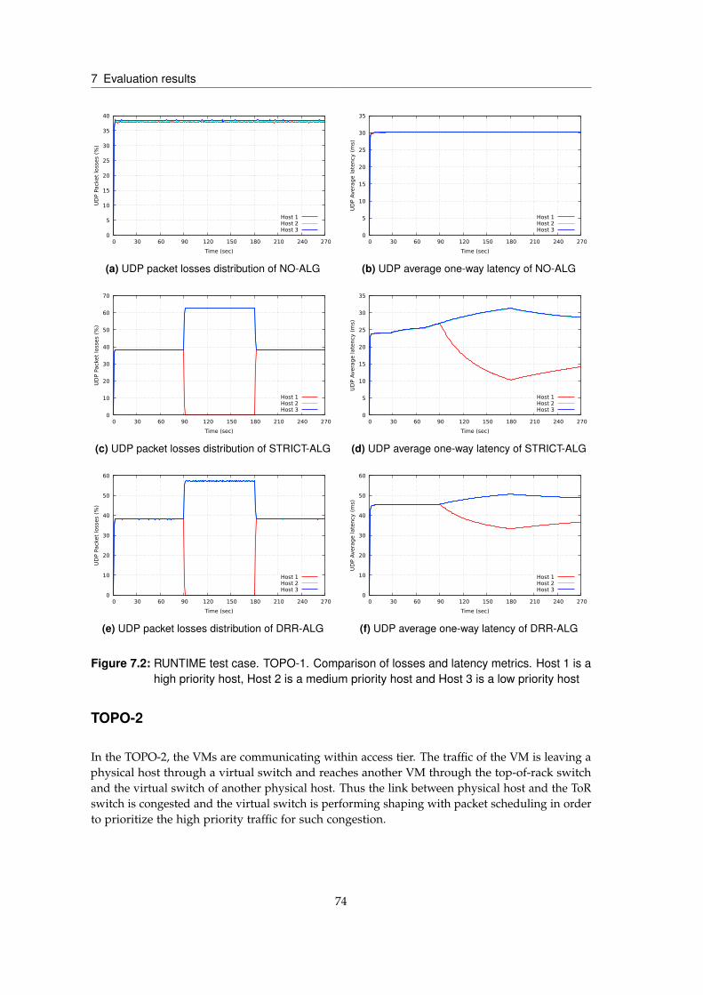
7 Evaluation results
0
5
10
15
20
25
30
35
40
0 30 60 90 120 150 180 210 240 270
UD
P P
ack
et
loss
es
(%)
Time (sec)
Host 1Host 2Host 3
(a) UDP packet losses distribution of NO-ALG
0
5
10
15
20
25
30
35
0 30 60 90 120 150 180 210 240 270
UD
P A
vera
ge late
ncy
(m
s)
Time (sec)
Host 1Host 2Host 3
(b) UDP average one-way latency of NO-ALG
0
10
20
30
40
50
60
70
0 30 60 90 120 150 180 210 240 270
UD
P P
ack
et
loss
es
(%)
Time (sec)
Host 1Host 2Host 3
(c) UDP packet losses distribution of STRICT-ALG
0
5
10
15
20
25
30
35
0 30 60 90 120 150 180 210 240 270
UD
P A
vera
ge late
ncy
(m
s)
Time (sec)
Host 1Host 2Host 3
(d) UDP average one-way latency of STRICT-ALG
0
10
20
30
40
50
60
0 30 60 90 120 150 180 210 240 270
UD
P P
ack
et
loss
es
(%)
Time (sec)
Host 1Host 2Host 3
(e) UDP packet losses distribution of DRR-ALG
0
10
20
30
40
50
60
0 30 60 90 120 150 180 210 240 270
UD
P A
vera
ge late
ncy
(m
s)
Time (sec)
Host 1Host 2Host 3
(f) UDP average one-way latency of DRR-ALG
Figure 7.2: RUNTIME test case. TOPO-1. Comparison of losses and latency metrics. Host 1 is ahigh priority host, Host 2 is a medium priority host and Host 3 is a low priority host
TOPO-2
In the TOPO-2, the VMs are communicating within access tier. The traffic of the VM is leaving aphysical host through a virtual switch and reaches another VM through the top-of-rack switchand the virtual switch of another physical host. Thus the link between physical host and the ToRswitch is congested and the virtual switch is performing shaping with packet scheduling in orderto prioritize the high priority traffic for such congestion.
74

7.1 RUNTIME test case
Similarly to the TOPO-1 results, figure 7.3 represents the bandwidth distribution for algorithmsapplied in the TOPO-2. For NO-ALG case, when packets are competing for the uplink of thevirtual switch, no traffic management is applied, thus TCP congestion control regulates itstransfer rate in the best-effort manner, as depicted in figure 7.3a. Applying UDP traffic witha constant rate that congests the uplink, the effective bandwidth is obtained for NO-ALG, asshown in figure 7.3b.
0
5
10
15
20
25
30
0 30 60 90 120 150 180 210 240 270
TCP B
andw
idth
(M
bps)
Time (sec)
Host 1Host 2Host 3
(a) TCP bandwidth distribution with NO-ALG
0
2
4
6
8
10
12
14
16
18
0 30 60 90 120 150 180 210 240 270
UD
P B
andw
idth
(M
bps)
Time (sec)
Host 1Host 2Host 3
(b) UDP bandwidth distribution with NO-ALG
0
5
10
15
20
25
30
0 30 60 90 120 150 180 210 240 270
TCP B
andw
idth
(M
bps)
Time (sec)
Host 1Host 2Host 3
(c) TCP bandwidth distribution with STRICT-ALG
0
5
10
15
20
25
30
0 30 60 90 120 150 180 210 240 270
UD
P B
andw
idth
(M
bps)
Time (sec)
Host 1Host 2Host 3
(d) UDP bandwidth distribution with STRICT-ALG
0
5
10
15
20
25
30
0 30 60 90 120 150 180 210 240 270
TCP B
andw
idth
(M
bps)
Time (sec)
Host 1Host 2Host 3
(e) TCP bandwidth distribution with DRR-ALG
0
5
10
15
20
25
30
0 30 60 90 120 150 180 210 240 270
UD
P B
andw
idth
(M
bps)
Time (sec)
Host 1Host 2Host 3
(f) UDP bandwidth distribution with DRR-ALG
Figure 7.3: RUNTIME test case. TOPO-2. Comparison of bandwidth distribution. Host 1 is a highpriority host, Host 2 is a medium priority host and Host 3 is a low priority host
When the traffic management is applied, the traffic is shaped and later the prioritization schemeis active. At initial stage, STRICT-ALG shapes TCP traffic better and faster than DRR-ALG, whencomparing the bandwidth distribution in figures 7.3c and 7.3e. This is again due to output buffer
75

7 Evaluation results
occupancy, as explained for TOPO-1 results. Moreover, higher number of switches and thusbuffers, destabilizes the shaping more, since it takes longer time for TCP congestion control todetect the losses and regulate its transmission rate. As a result, the stable period of bandwidthdistribution is prolonged to the 30th second of the experiment.
Once the prioritization is enabled at the 90th second, STRICT-ALG provides the stable distribution.For DRR-ALG, on the other hand, it is unstable due to the burstiness of high priority queue, asin TOPO-1. Furthermore, higher number of switch processes and threads also implies contextswitching between them. Therefore, the dequeueing is suspended for some of the switches,creating fluctuations even for STRICT-ALG. However, with UDP, shown in figures 7.3d and 7.3f,both algorithms equally shape and prioritize the traffic, and DRR-ALG utilizes low prioritiesslightly better with 11 Mbps versus 9.7 Mbps of STRICT-ALG.
Without traffic management, high priority traffic is exposed to the packet losses, as depicted infigure 7.4a. When the prioritization is enabled in such a way that the allocated bandwidth forhigh priority host sustains its transmission rate, no losses occur. This is depicted in figure 7.4cfor STRICT-ALG and figure 7.4e for DRR-ALG. Both eliminate the losses for high priority traffic,once the prioritization is activated, and increase the losses for the lower priorities up to 63% forSTRICT-ALG and 58% for DRR-ALG. DRR-ALG has less losses for lower priorities due to higherutilization.
Since the number of hops is increased for this topology and link capacity is decreased comparedto the TOPO-1, the average one-way latency is increased. For NO-ALG case, it is increased to60-64 ms, as shown in figure 7.4b. The average latency of STRICT-ALG initially is 48-50 ms.During prioritization phase, the latency of high priority traffic is dropped to 20 ms and for lowerpriorities, it is increased to 60 ms, as depicted in figure 7.4d. After disabling prioritization, theaverage latency for high priority is monotonously increasing, whereas for lower priorities, it isdecreasing. For DRR-ALG, the behavior is similar, shown in figure 7.4f, but with higher latencyvalues, due to higher queueing delay. Before prioritization, the VMs experience average latencyof 93 ms. During prioritization, it is increasing up to 106 ms for lower priorities and decreasingto 71 ms for high priority.
TOPO-3
In this tree topology the VMs are communicating across the aggregation switch. The packets of aVM are traversing from the virtual switch it is attached to, to the virtual switch of the other halfof the tree. The links that connect the physical host and the ToR switch are congested, as well asthe links that connect ToR switch with the aggregation switch. For the latter, the link capacity isdoubled, as for the former, the traffic management is applied.
Figures 7.5a and 7.5b represent the bandwidth distribution for TCP and UDP connectivity ofthe VMs respectively, when neither shaping nor packet scheduling is applied and best-effortapproach is undertaken.
When shaping and packet scheduling are applied with STRICT-ALG, similar behavior, as withthe previous topologies, has obtained. However, higher number of processes and threads createsdistortions for the bandwidth distribution of the TCP traffic, as presented in figure 7.5c, due
76
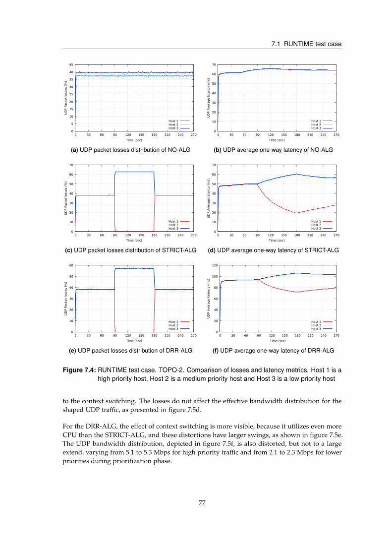
7.1 RUNTIME test case
0
5
10
15
20
25
30
35
40
45
0 30 60 90 120 150 180 210 240 270
UD
P P
ack
et
loss
es
(%)
Time (sec)
Host 1Host 2Host 3
(a) UDP packet losses distribution of NO-ALG
0
10
20
30
40
50
60
70
0 30 60 90 120 150 180 210 240 270
UD
P A
vera
ge late
ncy
(m
s)
Time (sec)
Host 1Host 2Host 3
(b) UDP average one-way latency of NO-ALG
0
10
20
30
40
50
60
70
0 30 60 90 120 150 180 210 240 270
UD
P P
ack
et
loss
es
(%)
Time (sec)
Host 1Host 2Host 3
(c) UDP packet losses distribution of STRICT-ALG
0
10
20
30
40
50
60
70
0 30 60 90 120 150 180 210 240 270
UD
P A
vera
ge late
ncy
(m
s)
Time (sec)
Host 1Host 2Host 3
(d) UDP average one-way latency of STRICT-ALG
0
10
20
30
40
50
60
0 30 60 90 120 150 180 210 240 270
UD
P P
ack
et
loss
es
(%)
Time (sec)
Host 1Host 2Host 3
(e) UDP packet losses distribution of DRR-ALG
0
20
40
60
80
100
120
0 30 60 90 120 150 180 210 240 270
UD
P A
vera
ge late
ncy
(m
s)
Time (sec)
Host 1Host 2Host 3
(f) UDP average one-way latency of DRR-ALG
Figure 7.4: RUNTIME test case. TOPO-2. Comparison of losses and latency metrics. Host 1 is ahigh priority host, Host 2 is a medium priority host and Host 3 is a low priority host
to the context switching. The losses do not affect the effective bandwidth distribution for theshaped UDP traffic, as presented in figure 7.5d.
For the DRR-ALG, the effect of context switching is more visible, because it utilizes even moreCPU than the STRICT-ALG, and these distortions have larger swings, as shown in figure 7.5e.The UDP bandwidth distribution, depicted in figure 7.5f, is also distorted, but not to a largeextend, varying from 5.1 to 5.3 Mbps for high priority traffic and from 2.1 to 2.3 Mbps for lowerpriorities during prioritization phase.
77

7 Evaluation results
0
1
2
3
4
5
6
0 30 60 90 120 150 180 210 240 270 300
TCP B
andw
idth
(M
bps)
Time (sec)
Host 1Host 2Host 3
(a) TCP bandwidth distribution with NO-ALG
0
500
1
2
2
2
3
4
0 30 60 90 120 150 180 210 240 270
UD
P B
andw
idth
(M
bps)
Time (sec)
Host 1Host 2Host 3
(b) UDP bandwidth distribution with NO-ALG
0
1
2
3
4
5
6
7
0 30 60 90 120 150 180 210 240 270 300
TCP B
andw
idth
(M
bps)
Time (sec)
Host 1Host 2Host 3
(c) TCP bandwidth distribution with STRICT-ALG
0
1
2
3
4
5
6
0 30 60 90 120 150 180 210 240 270
UD
P B
andw
idth
(M
bps)
Time (sec)
Host 1Host 2Host 3
(d) UDP bandwidth distribution with STRICT-ALG
0
1
2
3
4
5
6
7
8
0 30 60 90 120 150 180 210 240 270 300
TCP B
andw
idth
(M
bps)
Time (sec)
Host 1Host 2Host 3
(e) TCP bandwidth distribution with DRR-ALG
0
1
2
3
4
5
6
0 30 60 90 120 150 180 210 240 270
UD
P B
andw
idth
(M
bps)
Time (sec)
Host 1Host 2Host 3
(f) UDP bandwidth distribution with DRR-ALG
Figure 7.5: RUNTIME test case. TOPO-3. Comparison of bandwidth distribution. Host 1 is a highpriority host, Host 2 is a medium priority host and Host 3 is a low priority host
Figure 7.6a presents distribution of the packet losses over time for NO-ALG. The distortionsagain persist due to higher number of switches. Same applies to the DRR-ALG, the packet lossesof which is shown in figure 7.6e. The prioritization yet remains functional, removing the lossesfor high priority traffic, as in case of STRICT-ALG, depicted in figure 7.6c.
The average one-way latency is again increased for all algorithms, because TOPO-3 involveshigher number of hops. For best-effort approach, it saturates at 315 ms (figure 7.6b). Whenprioritization is enabled, STRICT-ALG decreases average latency from 250 ms to 100 ms for highpriority, while increasing lower priorities up to 300 ms (figure 7.6d). DRR-ALG has higher latency
78

7.1 RUNTIME test case
0
5
10
15
20
25
30
35
40
45
0 30 60 90 120 150 180 210 240 270
UD
P P
ack
et
loss
es
(%)
Time (sec)
Host 1Host 2Host 3
(a) UDP packet losses distribution of NO-ALG
0
50
100
150
200
250
300
350
0 30 60 90 120 150 180 210 240 270
UD
P A
vera
ge late
ncy
(m
s)
Time (sec)
Host 1Host 2Host 3
(b) UDP average one-way latency of NO-ALG
0
10
20
30
40
50
60
70
0 30 60 90 120 150 180 210 240 270
UD
P P
ack
et
loss
es
(%)
Time (sec)
Host 1Host 2Host 3
(c) UDP packet losses distribution of STRICT-ALG
0
50
100
150
200
250
300
350
0 30 60 90 120 150 180 210 240 270
UD
P A
vera
ge late
ncy
(m
s)
Time (sec)
Host 1Host 2Host 3
(d) UDP average one-way latency of STRICT-ALG
0
10
20
30
40
50
60
70
0 30 60 90 120 150 180 210 240 270
UD
P P
ack
et
loss
es
(%)
Time (sec)
Host 1Host 2Host 3
(e) UDP packet losses distribution of DRR-ALG
0
100
200
300
400
500
600
0 30 60 90 120 150 180 210 240 270
UD
P A
vera
ge late
ncy
(m
s)
Time (sec)
Host 1Host 2Host 3
(f) UDP average one-way latency of DRR-ALG
Figure 7.6: RUNTIME test case. TOPO-3. Comparison of losses and latency metrics. Host 1 is ahigh priority host, Host 2 is a medium priority host and Host 3 is a low priority host
due to higher queue delay and it goes from 467 ms down to 347 ms for high priority trafficduring prioritization phase, and increase up to 520 ms for the traffic of lower priorities (figure7.6f).
It can be also noted that for TOPO-3, the latency saturation process starts later than in TOPO-1 and TOPO-2. Numerically, around 30 seconds from the beginning of the experiment forTOPO-3, 15 seconds for TOPO-2 and 10 seconds for TOPO-1. This is due to the involvementof higher number of forwarding devices that can buffer more packets along the route between
79

7 Evaluation results
communicating VMs and decrease of link rates, thus the timespan to saturate the buffers of thedevices is increasing.
7.2 PROACTIVE test case
TOPO-1
PROACTIVE test case represents the case, where the traffic management with prioritization isenabled during the experiment. Lower priorities VMs generate the traffic, but high priority trafficis generated after 90 seconds from the start and lasts for another 90 seconds. In TOPO-1, VMsare communicating within a physical host. The virtual switch prioritizes the high priority traffic,giving larger share of bandwidth of the link that connects the switch and the server VM.
At the beginning of the experiment, only lower priorities generate the traffic. Figure 7.7a showsTCP traffic that is managed in the best-effort manner, as defined with NO-ALG case without anyshaping mechanism. Once the high priority traffic appears in the network at the 90th second,the absence of the traffic management does not prioritize it, and the TCP congestion controlcontinues to adapt its rate. For UDP traffic, depicted in figure 7.7b, the bandwidth is sharedfairly between participating VMs with small variations, since the UDP transfer rate is the samefor all VMs.
When the traffic management is handled using STRICT-ALG, in the condition of full linkutilization, the proactivity is not possible, as explained in section 6.3. Therefore the rates for fairshare are set for lower priorities traffic at the exact time, when the high priority traffic appearsand leaves the network. The TCP traffic is shaped, as shown in figure 7.7c with slight variations,and high priority traffic is prioritized during its existence. The behavior is similar for trafficgenerated by UDP, but without any visible variations, as depicted in figure 7.7d.
The prioritization scheme is proactively set with DRR-ALG and no control plane interactionsare needed. In figure 7.7e, the traffic is generated using TCP and shaped fairly distributingthe bandwidth. Due to the involvement of two low priority traffic, the implicit service rate oftheir respective egress buffers is half of the link rate. The egress buffers are then served in adeficit round-robin manner and TCP increases its transmission rate, until the saturation of theoutput buffer. Once the output buffer is freeing its space, the burst of the packets from one ofthe egress buffers is dequeued according to the quantum values, while another egress buffer isstalled, which further increases its queueing delay. As a result, the later TCP flow decreases itstransmission rate, while TCP of the first flow increases its rate until the output buffer saturationis reached again. At some point, the roles are changed, and the first TCP flow has decrease intransmission rate for the same reason. Therefore, the fluctuations are observed for the timespanwithout high priority traffic.
When high priority traffic appears, the output buffer is occupied by low priority packets. Thiscauses high priority queue to be stalled and later bursts its packets into the buffer, delayingthe service of low priority queues. The low priority TCP flows have then their transmissionrate decreased, while for high priority flow, it is increased up to the allocated bandwidth for
80
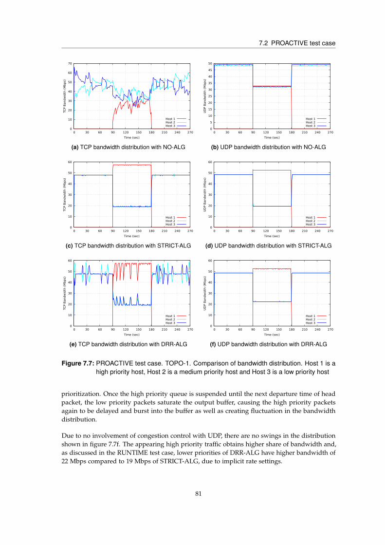
7.2 PROACTIVE test case
0
10
20
30
40
50
60
70
0 30 60 90 120 150 180 210 240 270
TCP B
andw
idth
(M
bps)
Time (sec)
Host 1Host 2Host 3
(a) TCP bandwidth distribution with NO-ALG
0
5
10
15
20
25
30
35
40
45
50
0 30 60 90 120 150 180 210 240 270
UD
P B
andw
idth
(M
bps)
Time (sec)
Host 1Host 2Host 3
(b) UDP bandwidth distribution with NO-ALG
0
10
20
30
40
50
60
0 30 60 90 120 150 180 210 240 270
TCP B
andw
idth
(M
bps)
Time (sec)
Host 1Host 2Host 3
(c) TCP bandwidth distribution with STRICT-ALG
0
10
20
30
40
50
60
0 30 60 90 120 150 180 210 240 270
UD
P B
andw
idth
(M
bps)
Time (sec)
Host 1Host 2Host 3
(d) UDP bandwidth distribution with STRICT-ALG
0
10
20
30
40
50
60
0 30 60 90 120 150 180 210 240 270
TCP B
andw
idth
(M
bps)
Time (sec)
Host 1Host 2Host 3
(e) TCP bandwidth distribution with DRR-ALG
0
10
20
30
40
50
60
0 30 60 90 120 150 180 210 240 270
UD
P B
andw
idth
(M
bps)
Time (sec)
Host 1Host 2Host 3
(f) UDP bandwidth distribution with DRR-ALG
Figure 7.7: PROACTIVE test case. TOPO-1. Comparison of bandwidth distribution. Host 1 is ahigh priority host, Host 2 is a medium priority host and Host 3 is a low priority host
prioritization. Once the high priority queue is suspended until the next departure time of headpacket, the low priority packets saturate the output buffer, causing the high priority packetsagain to be delayed and burst into the buffer as well as creating fluctuation in the bandwidthdistribution.
Due to no involvement of congestion control with UDP, there are no swings in the distributionshown in figure 7.7f. The appearing high priority traffic obtains higher share of bandwidth and,as discussed in the RUNTIME test case, lower priorities of DRR-ALG have higher bandwidth of22 Mbps compared to 19 Mbps of STRICT-ALG, due to implicit rate settings.
81

7 Evaluation results
For the appearing high priority traffic, the packet losses should be minimized. Hence, withouttraffic management, the high priority is exposed to the losses, as depicted in figure 7.8a from 90thto 180th seconds, having 37% of losses. Figures 7.8c and 7.8e show no losses for high prioritytraffic caused by traffic management with STRICT-ALG and DRR-ALG respectively. At the sametime, the losses for lower priorities are increased: in STRICT-ALG up to 63% and in DRR-ALGup to 58%. The latter has less losses for lower priorities due to higher UDP bandwidth comparedto the STRICT-ALG.
0
5
10
15
20
25
30
35
40
0 30 60 90 120 150 180 210 240 270
UD
P P
ack
et
loss
es
(%)
Time (sec)
Host 1Host 2Host 3
(a) UDP packet losses distribution of NO-ALG
0
5
10
15
20
25
30
35
0 30 60 90 120 150 180 210 240 270
UD
P A
vera
ge late
ncy
(m
s)
Time (sec)
Host 1Host 2Host 3
(b) UDP average one-way latency of NO-ALG
0
10
20
30
40
50
60
70
0 30 60 90 120 150 180 210 240 270
UD
P P
ack
et
loss
es
(%)
Time (sec)
Host 1Host 2Host 3
(c) UDP packet losses distribution of STRICT-ALG
0
5
10
15
20
25
30
0 30 60 90 120 150 180 210 240 270
UD
P A
vera
ge late
ncy
(m
s)
Time (sec)
Host 1Host 2Host 3
(d) UDP average one-way latency of STRICT-ALG
0
10
20
30
40
50
60
0 30 60 90 120 150 180 210 240 270
UD
P P
ack
et
loss
es
(%)
Time (sec)
Host 1Host 2Host 3
(e) UDP packet losses distribution of DRR-ALG
0
5
10
15
20
25
30
35
40
45
0 30 60 90 120 150 180 210 240 270
UD
P A
vera
ge late
ncy
(m
s)
Time (sec)
Host 1Host 2Host 3
(f) UDP average one-way latency of DRR-ALG
Figure 7.8: PROACTIVE test case. TOPO-1. Comparison of losses and latency metrics. Host 1 isa high priority host, Host 2 is a medium priority host and Host 3 is a low priority host
The results of the average one-way latency for NO-ALG is presented in figure 7.8b. Withouttraffic management, the average latency is the same for lower priorities and equal to 29-30 ms.
82

7.2 PROACTIVE test case
The arrival of high priority traffic keeps the latency for all priorities at the same values, althoughintuitively the latency should be increased, since number of communicating VMs is increased.The losses are indeed increased, however, the latency is measured for the packets that are notdropped, thus higher number of communicating hosts does not effect the latency.
With STRICT-ALG, the drastic change of the latency is observed in figure 7.8d, rapidly decayingfrom 11 ms to the 0.2 ms. The starting point of 11 ms is due to the occupancy of the inputand output FIFO buffers (section 4.1.3) with the packets of lower priorities and the rapid decayis due to the lowest queue delays compared to the NO-ALG and DRR-ALG (figure 5.4). Theaverage latency for lower priorities increases from 21 ms to 26 ms, when the high priority trafficis generated. DRR-ALG in this experiment reaches 26 ms of constant average latency for highpriority, and for lower priorities the latency gradually increases from 36 ms to 43 ms, as shownin figure 7.8f. The average latency is higher due to the higher queue delay, in comparison withSTRICT-ALG, and is not decaying, because firstly the buffers of the switch are occupied withlower priorities packets and belated dequeue of high priority packets does not allow to occupythe output buffer at the scheduled departure time, as discussed in section 5.2.
TOPO-2
In this topology, NO-ALG demonstrates best-effort manner, shown in figures 7.9a and 7.9b, whenno traffic management is applied for the uplink of the virtual switch. At the time of appearing,the high priority TCP and UDP traffic do not obtain higher bandwidth. Comparing the cases,when traffic management is enabled, STRICT-ALG shapes the TCP traffic in a more stable waythan DRR-ALG, as depicted in figures 7.9c and 7.9e, since the rate limitation is explicit. Whenhigh priority TCP traffic occurs, both prioritize it by giving higher bandwidth share. With UDPtraffic (figures 7.9d and 7.9f), their behavior is similar, but DRR-ALG slightly better utilizes thelink with lower priorities.
The loss distribution is similar to TOPO-1. NO-ALG does not handle losses for high prioritytraffic, as shown in figure 7.10a. Whereas with enabled traffic management, no losses occurfor high priority traffic in STRICT-ALG case, as depicted in figure 7.10c. In DRR-ALG case,insignificant jumps in losses (less than 0.8%) at 137th, 148th and 166th seconds occur, as shownin figure 7.10e.
In the TOPO-2, with increased number of hops and decreased capacity of the links, the latency isalso increased by the same amount as in RUNTIME test case. Figure 7.10b presents the one-wayaverage latency, when no traffic management is applied, being 60-62 ms for all priorities. Whenhigh priority traffic appears, the initial average latency obtained is 50 ms and then it rapidlydecays to 1 ms for the STRICT-ALG. The lower priorities experience steady increase in latencyfrom 40 to 51 ms for the period of high priority traffic generation, as shown in figure 7.10d. TheDRR-ALG’s initial latency value of 53 ms for high priority traffic remains the same without anydecay, as depicted in figure 7.10f, due to the output buffer occupancy. Simultaneously, the latencyof the lower priorities increases from 75 ms to 89 ms.
83

7 Evaluation results
0
5
10
15
20
25
30
35
0 30 60 90 120 150 180 210 240 270
TCP B
andw
idth
(M
bps)
Time (sec)
Host 1Host 2Host 3
(a) TCP bandwidth distribution with NO-ALG
0
5
10
15
20
25
0 30 60 90 120 150 180 210 240 270
UD
P B
andw
idth
(M
bps)
Time (sec)
Host 1Host 2Host 3
(b) UDP bandwidth distribution with NO-ALG
0
5
10
15
20
25
30
0 30 60 90 120 150 180 210 240 270
TCP B
andw
idth
(M
bps)
Time (sec)
Host 1Host 2Host 3
(c) TCP bandwidth distribution with STRICT-ALG
0
5
10
15
20
25
30
0 30 60 90 120 150 180 210 240 270
UD
P B
andw
idth
(M
bps)
Time (sec)
Host 1Host 2Host 3
(d) UDP bandwidth distribution with STRICT-ALG
0
5
10
15
20
25
30
0 30 60 90 120 150 180 210 240 270
TCP B
andw
idth
(M
bps)
Time (sec)
Host 1Host 2Host 3
(e) TCP bandwidth distribution with DRR-ALG
0
5
10
15
20
25
30
0 30 60 90 120 150 180 210 240 270
UD
P B
andw
idth
(M
bps)
Time (sec)
Host 1Host 2Host 3
(f) UDP bandwidth distribution with DRR-ALG
Figure 7.9: PROACTIVE test case. TOPO-2. Comparison of bandwidth distribution. Host 1 is ahigh priority host, Host 2 is a medium priority host and Host 3 is a low priority host
TOPO-3
TOPO-3 involves greater number of switches and hops that, as with RUNTIME test case, causesthe distortions to the performance metrics, especially visible with TCP traffic.
When the traffic is not regulated, the best-effort bandwidth distributions, shown in figures7.11a and 7.11b, are obtained, representing NO-ALG case. Occurring high priority traffic is notprioritized, whereas with STRICT-ALG it is shaped with some distortions and it occupies higherbandwidth compared to the lower priories, as depicted in figures 7.11c and 7.11d.
84

7.2 PROACTIVE test case
0
5
10
15
20
25
30
35
40
0 30 60 90 120 150 180 210 240 270
UD
P P
ack
et
loss
es
(%)
Time (sec)
Host 1Host 2Host 3
(a) UDP packet losses distribution of NO-ALG
0
10
20
30
40
50
60
70
0 30 60 90 120 150 180 210 240 270
UD
P A
vera
ge late
ncy
(m
s)
Time (sec)
Host 1Host 2Host 3
(b) UDP average one-way latency of NO-ALG
0
10
20
30
40
50
60
70
0 30 60 90 120 150 180 210 240 270
UD
P P
ack
et
loss
es
(%)
Time (sec)
Host 1Host 2Host 3
(c) UDP packet losses distribution of STRICT-ALG
0
10
20
30
40
50
60
0 30 60 90 120 150 180 210 240 270
UD
P A
vera
ge late
ncy
(m
s)
Time (sec)
Host 1Host 2Host 3
(d) UDP average one-way latency of STRICT-ALG
0
10
20
30
40
50
60
0 30 60 90 120 150 180 210 240 270
UD
P P
ack
et
loss
es
(%)
Time (sec)
Host 1Host 2Host 3
(e) UDP packet losses distribution of DRR-ALG
0
10
20
30
40
50
60
70
80
90
0 30 60 90 120 150 180 210 240 270
UD
P A
vera
ge late
ncy
(m
s)
Time (sec)
Host 1Host 2Host 3
(f) UDP average one-way latency of DRR-ALG
Figure 7.10: PROACTIVE test case. TOPO-2. Comparison of losses and latency metrics. Host 1is a high priority host, Host 2 is a medium priority host and Host 3 is a low priorityhost
The TCP traffic is not properly shaped with large swings in DRR-ALG case due to higher numberof the switch processes participating in traffic forwarding. However, the prioritization is visiblein figures 7.11e and 7.11f, upon the occurrence of high priority traffic, although for TCP trafficthe distortions are more intense.
When it comes to the packet losses during UDP traffic generation, similarly to other simulatedtopologies of this test case, the best-effort approach does not prevent high priority traffic fromlosses, as shown in figure 7.12a. Whereas, with traffic management using STRICT-ALG and
85

7 Evaluation results
0
1
2
3
4
5
6
7
8
0 30 60 90 120 150 180 210 240 270 300
TCP B
andw
idth
(M
bps)
Time (sec)
Host 1Host 2Host 3
(a) TCP bandwidth distribution with NO-ALG
0
500
1
2
2
2
3
4
4
5
5
0 30 60 90 120 150 180 210 240 270
UD
P B
andw
idth
(M
bps)
Time (sec)
Host 1Host 2Host 3
(b) UDP bandwidth distribution with NO-ALG
0
1
2
3
4
5
6
7
0 30 60 90 120 150 180 210 240 270 300
TCP B
andw
idth
(M
bps)
Time (sec)
Host 1Host 2Host 3
(c) TCP bandwidth distribution with STRICT-ALG
0
1
2
3
4
5
6
0 30 60 90 120 150 180 210 240 270
UD
P B
andw
idth
(M
bps)
Time (sec)
Host 1Host 2Host 3
(d) UDP bandwidth distribution with STRICT-ALG
0
1
2
3
4
5
6
7
8
9
0 30 60 90 120 150 180 210 240 270 300
TCP B
andw
idth
(M
bps)
Time (sec)
Host 1Host 2Host 3
(e) TCP bandwidth distribution with DRR-ALG
0
1
2
3
4
5
6
0 30 60 90 120 150 180 210 240 270
UD
P B
andw
idth
(M
bps)
Time (sec)
Host 1Host 2Host 3
(f) UDP bandwidth distribution with DRR-ALG
Figure 7.11: PROACTIVE test case. TOPO-3. Comparison of bandwidth distribution. Host 1 is ahigh priority host, Host 2 is a medium priority host and Host 3 is a low priority host
DRR-ALG, the losses are not introduced due to applied prioritization scheme, as shown infigures 7.12c and 7.12e. Yet, the loss distribution over time of DRR-ALG is slightly distorted andnegligible loss of 0.89% is observed at 147th second of the experiment.
The latency is again increased, because the traffic needs to propagate through greater number offorwarding devices. This way, the average one-way latency for lower priorities saturates at 303ms for NO-ALG case and 313 ms for appearing high priority traffic, as shown in figure 7.12b.For STRICT-ALG case, the average latency distribution for lower priorities saturates at 162 msbefore high priority traffic appears. After that, the latency increases up to 227 ms. High priority
86

7.2 PROACTIVE test case
0
5
10
15
20
25
30
35
40
0 30 60 90 120 150 180 210 240 270
UD
P P
ack
et
loss
es
(%)
Time (sec)
Host 1Host 2Host 3
(a) UDP packet losses distribution of NO-ALG
0
50
100
150
200
250
300
350
0 30 60 90 120 150 180 210 240 270
UD
P A
vera
ge late
ncy
(m
s)
Time (sec)
Host 1Host 2Host 3
(b) UDP average one-way latency of NO-ALG
0
10
20
30
40
50
60
70
0 30 60 90 120 150 180 210 240 270
UD
P P
ack
et
loss
es
(%)
Time (sec)
Host 1Host 2Host 3
(c) UDP packet losses distribution of STRICT-ALG
0
50
100
150
200
250
0 30 60 90 120 150 180 210 240 270
UD
P A
vera
ge late
ncy
(m
s)
Time (sec)
Host 1Host 2Host 3
(d) UDP average one-way latency of STRICT-ALG
0
10
20
30
40
50
60
0 30 60 90 120 150 180 210 240 270
UD
P P
ack
et
loss
es
(%)
Time (sec)
Host 1Host 2Host 3
(e) UDP packet losses distribution of DRR-ALG
0
50
100
150
200
250
300
350
400
450
0 30 60 90 120 150 180 210 240 270
UD
P A
vera
ge late
ncy
(m
s)
Time (sec)
Host 1Host 2Host 3
(f) UDP average one-way latency of DRR-ALG
Figure 7.12: PROACTIVE test case. TOPO-3. Comparison of losses and latency metrics. Host 1is a high priority host, Host 2 is a medium priority host and Host 3 is a low priorityhost
traffic initially experiences the latency of 128 ms, and when the buffers of the forwarding devicesare freeing up from the excess of lower priorities packets, the latency is decaying up to 4 ms, asdepicted in figure 7.12d. As shown in figure 7.12f for average latency distribution of DRR-ALG,the latency of the lower priorities are slowly reaching 373 ms, before the high priority trafficoccurs, and once it leaves, 443 ms of average latency is obtained. The latency of the high prioritytraffic is unchanged during generation with the value of 278 ms, indicating again the queue delaycaused by the output buffer occupancy.
87

7 Evaluation results
Like with the RUNTIME test case, the latency saturation starts later for TOPO-3 than for TOPO-1and TOPO-2 due to higher number of forwarding devices, decrease in link rates and higheroverall buffer size in the network.
7.3 MPI test case
TOPO-1
For this test case, low priority hosts are running iperf generating TCP or UDP traffic, while theMPI application, which measures ping-pong latency, is deployed on the pair of high priority hosts.The MPI processes consume 200% of CPU, as explained in section 6.1.3. Thus, the remainingCPU share is allocated for switch processes and affects their performance.
In this topology, Host 4 is an iperf-server, as well as the host running the MPI application togetherwith Host 1, where iperf is disabled. Hosts 2 and 3 are generating TCP or UDP traffic. The resultsof average MPI ping-pong latency for different message sizes are then obtained.
Figure 7.13 represents the results of average latencies for NO-ALG, STRICT-ALG and DRR-ALG,when the low priority hosts are generating TCP traffic. The performance of DRR-ALG is slightlybetter than the performance of NO-ALG, which implies no traffic management, over all messagesizes, except for 2, 16 and 16384 bytes messages. However, both perform way worse than theSTRICT-ALG. Numerically, as an example, for message size of 1024 bytes, NO-ALG has 43.4 ms,DRR-ALG has 39.3 ms and STRICT-ALG has 0.59 ms.
To explain this, output buffer occupancy needs to be recalled, as described in section 5.2. InNO-ALG and DRR-ALG, when low priority hosts generate traffic, the output buffer of a switchis occupied by low priority packets. Whereas for STRICT-ALG case, low priority packets arealways delayed, according to the rates of low priority queues. Hence, the output buffer is notsaturated with low priority packets, and queue delay for high priority traffic is thus minimized.
TCP, unlike UDP that "mercilessly" congests the links, is a fair protocol that decreases thetransmission rate in case of congestions. Thus, when low priority hosts are generating UDPtraffic, the ping-pong latency is increased compared to the TCP case, as depicted in figure 7.14.This, however, does not affect the latency for STRICT-ALG for the above mentioned reasons inoutput buffer occupancy and STRICT-ALG outperforms NO-ALG and DRR-ALG. The UDP trafficgeneration consumes less CPU, due to unidirectional communication, as discussed in section6.4, hence the prioritization of DRR-ALG allows to have less latency compared to NO-ALG byhaving more processing power for the scheduling. For the same message size of 1024 bytes, theaverage latency for NO-ALG is 227 ms and for DRR-ALG is 192 ms, whereas for STRICT-ALG itis 0.98 ms.
88
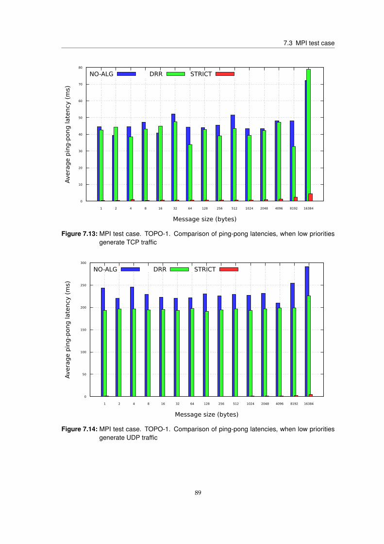
7.3 MPI test case
0
10
20
30
40
50
60
70
80
1 2 4 8 16 32 64 128 256 512 1024 2048 4096 8192 16384
Avera
ge p
ing
-pong
late
ncy
(m
s)
Message size (bytes)
NO-ALG DRR STRICT
Figure 7.13: MPI test case. TOPO-1. Comparison of ping-pong latencies, when low prioritiesgenerate TCP traffic
0
50
100
150
200
250
300
1 2 4 8 16 32 64 128 256 512 1024 2048 4096 8192 16384
Avera
ge p
ing
-pong
late
ncy
(m
s)
Message size (bytes)
NO-ALG DRR STRICT
Figure 7.14: MPI test case. TOPO-1. Comparison of ping-pong latencies, when low prioritiesgenerate UDP traffic
89

7 Evaluation results
TOPO-2
In the second topology, pair of high priority hosts, Host 1 and Host 4, are running the MPIlatency measuring application with disabled iperf, while other hosts are generating TCP or UDPtraffic. The results of the average latencies, when TCP-based low priority traffic is generated, arepresented in figure 7.15. The latency for DRR-ALG approaches the latency for NO-ALG, beingeven higher for some message sizes. This is because MPI processes take over most of CPU share,and therefore DRR-ALG lacks of CPU consumption to sustain its scheduling, which increases theprocessing time and prolongs dequeueing. Similarly to TOPO-1, STRICT-ALG performs the besthaving latencies below 11 ms. This is again due to the output buffer occupancy and delay of lowpriority traffic.
0
50
100
150
200
250
300
350
1 2 4 8 16 32 64 128 256 512 1024 2048 4096 8192 16384
Avera
ge p
ing
-pong
late
ncy
(m
s)
Message size (bytes)
NO-ALG DRR STRICT
Figure 7.15: MPI test case. TOPO-2. Comparison of ping-pong latencies, when low prioritiesgenerate TCP traffic
For low priority UDP traffic, the performance of DRR-ALG is again better because of less requiredCPU consumption, and this reflects in lesser latency compared to NO-ALG over all messagesizes, except for 1 and 4096 bytes, as shown in figure 7.16. The latencies for STRICT-ALG are thelowest.
TOPO-3
In the TOPO-3, only high priority hosts, Host 1 and Host 7, are running the MPI application,while other hosts are generating TCP or UDP traffic.
90

7.3 MPI test case
0
100
200
300
400
500
600
700
800
1 2 4 8 16 32 64 128 256 512 1024 2048 4096 8192 16384
Avera
ge p
ing
-pong
late
ncy
(m
s)
Message size (bytes)
NO-ALG DRR STRICT
Figure 7.16: MPI test case. TOPO-2. Comparison of ping-pong latencies, when low prioritiesgenerate UDP traffic
In this topology, higher number of switch processes and TCP acknowledgment traffic affectthe CPU consumption, which, in turn, reflects on the processing time of the packet scheduling.Thereby, the average latency of DRR-ALG is the highest among other scheduling cases for mostof the message sizes, except for 16, 32, 8192 and 16384 bytes, as shown in figure 7.17. The averagelatency for STRICT-ALG at most reaches 50 ms for 16384 bytes messages, whereas, with the samemessage size, it is 1.7 s and 1.4 s for NO-ALG and DRR-ALG respectively.
For UDP traffic of low priority hosts, the average latency is increased for MPI communication,however, the prioritization improves its performance, as shown in figure 7.18, when comparedto the case without traffic management. Over all message sizes, the latencies of DRR-ALG andSTRICT-ALG are lower, e.g. for message size of 16384 bytes, the latencies are, respectively, 2.6 sand 51 ms on average, while NO-ALG has 3.9 s.
It can be notices that in all considered topologies, when low priority hosts generate TCP traffic,DRR-ALG has the highest MPI ping-pong latency for small message sizes, e.g. 1, 2, 16 bytes, andlarge message sizes, e.g. 8192, 16384 bytes. For small messages, the possible explanation is thatsmall packets do not burst the output buffer, since a small packet already contains the wholemessage, thus the output buffer is always saturated by low priority traffic. Large messages, onthe other hand, are segmented into 6-10 packets due to the smaller size of MTU compared to themessage size. Therefore, high priority packets burst into the output buffer up to the point, whenthe output buffer is saturated or the departure time of a head packet has not yet come. It is thenpossible that the message transmission experiences multiple queue delays because of the highnumber of packets of one message in the egress buffer that are inconsistently dequeued.
91

7 Evaluation results
0
200.0*103
400.0*103
600.0*103
800.0*103
1.0*106
1.2*106
1.4*106
1.6*106
1.8*106
1 2 4 8 16 32 64 128 256 512 1024 2048 4096 8192 16384
Avera
ge p
ing
-pong
late
ncy
(μ
s)
Message size (bytes)
NO-ALG DRR STRICT
Figure 7.17: MPI test case. TOPO-3. Comparison of ping-pong latencies, when low prioritiesgenerate TCP traffic
0
500.0*103
1.0*106
1.5*106
2.0*106
2.5*106
3.0*106
3.5*106
4.0*106
4.5*106
1 2 4 8 16 32 64 128 256 512 1024 2048 4096 8192 16384
Avera
ge p
ing
-pong
late
ncy
(μ
s)
Message size (bytes)
NO-ALG DRR STRICT
Figure 7.18: MPI test case. TOPO-3. Comparison of ping-pong latencies, when low prioritiesgenerate UDP traffic
92

7.4 Discussion
7.4 Discussion
From the obtained results of bandwidth distribution, losses and average one-way and ping-ponglatencies for different test cases with and without traffic management, it became evident that:
• the traffic management indeed regulates the traffic, smoothing it up to desired rate. Without it,the bandwidth distribution fluctuates;
• the role of the traffic shaping and packet scheduling is important for bandwidth distribution.Choosing complex scheduling algorithm affects the performance of the software switches,especially for high transmission rates;
• prioritization schemes indeed improves the networking characteristics for high priority traffic,but with decrease in performance for low priority traffic;
• in the CPU limited environment, the simulation results are exposed to the distortions dueto higher number of emulated forwarding devices, link capacities and complexity of trafficmanagement algorithms;
When comparing traffic management, which was accomplished with STRICT-ALG and DRR-ALG,the stability and speed of TCP traffic shaping are clearly better for STRICT-ALG, although UDPtraffic shaping is comparable in terms of bandwidth allocation, but not latency. When applyingtraffic management for the improvement of MPI communication, it is clear that prioritizationdone with STRICT-ALG outperforms DRR-ALG in terms of ping-pong latency due to the delayof low priority queues, which does not allow to overrun the output buffer, and lower complexity.Whereas for DRR-ALG, the output buffers are occupied by low priority packets resulting inhigher queue delay. The major issue, however, with STRICT-ALG is the scalability. To elaboratethis, the number of control plane commands for bandwidth allocation will be calculated.
The condition was imposed that the links need to be fully utilized. Assume that there are Nvirtual switches and M virtual machines per switch, where, for simplicity, only one virtualmachine has high priority (P = 1) and initial network pre-configuration is made. Hence forRUNTIME test case, the control plane needs to send N ∗ M commands to shape the traffic forall VMs including prioritized VMs, whereas for DRR-ALG the traffic implicitly shaped usingpredefined quantum values, thus only commands for prioritization are needed: N ∗ P = N, forP = 1. So there is M times less commands that can be sent by the control plane and assuming 10VMs per physical host, 10 times less commands can be achieved.
The proactive bandwidth allocation is not possible with STRICT-ALG, if the shaping is requiredfor low priority traffic and the links should be utilized completely, as described in the PROACTIVEtest case. Therefore, if the prioritization scheme is proactively enabled, then the adjustments ofthe rates are needed, but only for low priorities, and the number of commands is decreasing toN ∗ (M − P) = N ∗ (M − 1), for P = 1. However, with DRR-ALG, traffic of any priority can beshaped and prioritized proactively utilizing the links without sending any further control planecommands. Though, if the traffic shaping is not required for lower priorities and the best-effortapproach is suitable, then STRICT-ALG can be used for bandwidth guarantee for high prioritytraffic and lower priorities will adaptively occupy the remaining of the bandwidth. Hence, being
93

7 Evaluation results
scalable, better buffer management for DRR-ALG needs to be addressed, as will be described inthe future work section.
As the summary and comparison of obtained results for each test case and topology, table 7.1 isprovided.
CharacteristicAlgorithm NO-ALG:
best-effortSTRICT-ALG:strict priority
DRR-ALG:RL-SP DRR
Prioritization No Yes YesShaping TCP traffic No Immediate, stable Slower, with fluctuationsShaping UDP traffic No Immediate, stable Immediate, stableLoss recovery No Yes Yes
One-way latency Highest LowestLower thanNO-ALG
Link utilization YesNeeds dynamic
allocation Yes
CPU consumption LowestHigher than
NO-ALG HighestScalability – No Yes
MPI ping-pong latency,(low priority TCP traffic) Highest Lowest
Slightly lower thanNO-ALG
MPI ping-pong latency,(low priority UDP traffic) Highest Lowest
Lower thanNO-ALG
Table 7.1: Summary of discussed results for RUNTIME, PROACTIVE and MPI test cases andcomparison of traffic management characteristics between NO-ALG, STRICT-ALG andDRR-ALG
94

8 Conclusion
The latency-critical services in the cloud infrastructure like HPC applications experience lowperformance due to lack of traffic regulation. The share of the network resources in the best-effortmanner creates unstable bandwidth distribution and increases latency for these services. Therole of traffic management in such infrastructure is hence of great importance. More specifically,the prioritization schemes are applied in order to allocate larger share of bandwidth using trafficshaping and packet scheduling.
In order to cope with highly dynamic topological changes, cloud providers employ programmablenetwork devices, the routes establishment of which are configurable at the runtime throughcentralized or distributed control plane. However, traffic management of these devices can notbe configured the same way and has limitations, e.g. OpenFlow protocol provides no interfacesfor traffic management and the interfaces of hardware appliances should be used, which leadsto the vendor lock-in problem. On the other hand, emerging data plane programmability withP4 language provides the right abstraction and constructs to implement the interfaces for theconfiguration of the device internals through control plane, including traffic manager.
This thesis work designs a conceptual traffic manager with the goals of complete link utilization,prioritization and scalability using rate limited strict priority with deficit round-robin (RL-SPDRR) packet scheduling algorithm. It is then implemented on the P4 software switch, bmv2, andis programmable through metadata-based interface. This way, the parameters of the algorithm,e.g. priority, rate and quantum, can be provisioned by a pipeline table, which, in turn, ispopulated by the control plane. Therefore, programmable traffic management using standardcontrol plane API is achieved.
The performance of implemented traffic manager is evaluated with the test cases, when prioriti-zation is enabled at the runtime and when it is proactively set, deployed on three topologies: star,tree with depth of 1 and tree with depth of 2. Each topology represents different communicationpatterns of VMs in a cloud infrastructure, which are inside a physical host, across a ToR switchand across an aggregation switch. The comparison is then made with the best-effort approachand the strict priority scheduling. Additionally an MPI ping-pong application is run and theping-pong latencies are measured.
The observation of shaping and prioritization stability, packet losses and latencies is considered.RL-SP DRR allocates the bandwidth for prioritized UDP traffic same way as the strict priority,better utilizing bandwidth for non-prioritized traffic. For TCP traffic, the bandwidth distributionis unstable due to the disproportional occupation of the output buffer, delaying the prioritizedpackets. As a consequence, RL-SP DRR fails to considerably drop the one-way and MPI ping-ponglatencies for prioritized traffic, performing better than best-effort approach, but is outperformed

8 Conclusion
by the strict priority. However, no packet losses are observed for prioritized traffic, as opposed tothe best-effort approach.
Nevertheless, traffic management with RL-SP DRR benefits in scalability and link utilization.Much fewer control plane commands are involved when prioritization needs to be made atthe runtime. Moreover, no control plane interactions are needed to sustain links utilization incontrast to dynamic rate distribution with strict priority, once preliminary prioritization schemeis established.
Future work
As a future work, the definitive improvements firstly need to be made in the buffer managementof the switch, since the output buffer stagnates high priority traffic, creating queue delays.Increasing size of the output buffer such that the high priority packets will be dequeued withoutbursts might decrease fluctuation, however, large buffer increases delays. Shorter buffer willbe overrun faster, thus allowing TCP congestion control to react faster on the losses. Therefore,having variable, or rather adaptive size of the output buffer might stabilize shaping and increaseresponsiveness.
Regarding the buffer occupancy, the guaranteed space for high priority packets in the outputbuffer can be proposed. When the low priority packets occupy some threshold space of theoutput buffer, the subsequent dequeue is suspended, not allowing to overrun the buffer so thathigh priority packets will not suffer. It is similar to rate limited strict priority and Ethernetpriority-based flow control, but the pause is based on buffer occupancy and held internally,rather than rate-based and between forwarding devices.
Another approach is to implement the output buffer as a priority queue. When the high prioritypacket is dequeued from the egress buffer, it will be placed not in the end of the output buffer,but in the head. For the software switch, this approach will decrease the queue delay, however,implementation on a hardware switch yet needs to be investigated.
As mentioned in the design discussions (section 3.4), the portability of the traffic manager is poor,since the introduced rate and quantum metadata are part of the architecture’s standard metadata.Thus, the core needs to be rewritten. It is a better option to use a P4 extern object that willinteract with traffic manager through its mechanism. It can be stateful, meaning that the trafficmanager will not be configured each time a packet arrives, but only when the configurationchanges really occur. Using extern object is expected to be more portable due it its decouplingfrom the switch architecture. For this case, the portable switch architecture (PSA) [106] can beused, since it explicitly defines the buffering queueing engine.
After the proper buffer management and portability, P4 switch and the traffic manager canbe synthesized on the programmable hardware, e.g. FPGA, to serve as a hardware offloadof network virtualization, similarly to Mellanox eSwitch. This gives the ability to fully definenetwork functionality using P4 programs with the performance closer to the hardware switches.Moreover, deployment of traffic manager on hardware will utilize spacial hardware parallelism.Thus the efficiency of packet scheduling algorithms, e.g. DRR, can be improved, since multiple
96

queues and ports can be served simultaneously without the involvement of sequential CPU. Withthis performance implication, the programmable and hardware-based traffic management can bea step forward to dynamically provision on-demand low latency communication in the cloudinfrastructure. After achieving such traffic management, further experiments can be made in thereal cloud infrastructure.
Additionally, this thesis work does not address the following use cases that need to be resolvedin the future:
1. The underutilization still occurs when only high priority traffic is generated, since it is ratelimited.
2. The undefined behavior for the cases when multiple high priority flows are competing forthe output port.
3. The unknown classification of high priority traffic from the user perspective.
4. Links failover and resiliency.
97


Appendices
1 P4 program for the switch
Below is the source code for P4 program used in the experiment setup.
#include <core.p4>#include <v1model.p4>
const bit <16> TYPE_IPV4 = 0x800;
/* Header definitions */typedef bit <9> egressSpec_t;typedef bit <48> macAddr_t;typedef bit <32> ip4Addr_t;typedef bit <3> priority_t;typedef bit <64> queue_rate_t;typedef bit <64> queue_quantum_t;
header ethernet_t macAddr_t dstAddr;macAddr_t srcAddr;bit <16> etherType;
header ipv4_t bit <4> version;bit <4> ihl;bit <8> diffserv;bit <16> totalLen;bit <16> identification;bit <3> flags;bit <13> fragOffset;bit <8> ttl;bit <8> protocol;bit <16> hdrChecksum;ip4Addr_t srcAddr;ip4Addr_t dstAddr;
struct metadata

Appendices
struct headers ethernet_t ethernet;ipv4_t ipv4;
/* Parser */parser MyParser(packet_in packet ,
out headers hdr ,inout metadata meta ,inout standard_metadata_t standard_metadata)
state start transition parse_ethernet;
state parse_ethernet packet.extract(hdr.ethernet);transition select(hdr.ethernet.etherType)
TYPE_IPV4: parse_ipv4;default: accept;
state parse_ipv4 packet.extract(hdr.ipv4);transition accept;
/* Ingress checksum verification *//* Empty , since no Layer 3 header modifications involved */control MyVerifyChecksum(inout headers hdr , inout metadata meta)
apply
/* Ingress pipeline processing */control MyIngress(inout headers hdr ,
inout metadata meta ,inout standard_metadata_t standard_metadata)
action drop() mark_to_drop ();
action ipv4_forward(macAddr_t dstAddr , egressSpec_t port) standard_metadata.egress_spec = port;
100

P4 program for the switch
hdr.ethernet.dstAddr = dstAddr;
table ipv4_lpm key =
hdr.ipv4.dstAddr: lpm;actions =
ipv4_forward;drop;NoAction;
size = 1024;default_action = drop();
action set_priority(priority_t prio , queue_rate_t queue_rate ,queue_quantum_t queue_quantum) standard_metadata.priority = prio;standard_metadata.queue_rate = queue_rate;standard_metadata.queue_quantum = queue_quantum;
table src_ip_prio key =
hdr.ipv4.srcAddr: lpm;actions =
set_priority;drop;NoAction;
size = 1024;default_action = drop();
apply if (hdr.ipv4.isValid ())
src_ip_prio.apply();ipv4_lpm.apply();
/* Egress pipeline processing */control MyEgress(inout headers hdr ,
inout metadata meta ,inout standard_metadata_t standard_metadata)
101

Appendices
apply
/* Egress checksum verification *//* Empty , since no Layer 3 header modifications involved */control MyComputeChecksum(inout headers hdr , inout metadata meta)
apply
/* Deparser */control MyDeparser(packet_out packet , in headers hdr)
apply packet.emit(hdr.ethernet);packet.emit(hdr.ipv4);
/* Switch instance */V1Switch(MyParser (),MyVerifyChecksum (),MyIngress (),MyEgress (),MyComputeChecksum (),MyDeparser ()) main;
Listing 1: The source of P4 program used in evaluation setup
In order to compile and run, either P4 tutorials [102] can be used or manually compiled and run,as in the following example:
# variables definitionsP4_SRC="p4-switch.p4"BUILD_NAME="p4-switch"P4C_ARGS="--p4runtime-file $BUILD_NAME.p4info --p4runtime-format text"
# compilationp4c-bm2-ss --p4v 16 $P4C_ARGS -o $BUILD_NAME.json $P4_SRC
# run switch processsudo simple_switch_grpc -i 1@$IFACE_1 -i 2@$IFACE_2 $BUILD_NAME.json
The implementation details of the targets implemented in this work, the compilation process andmeasurements can be found the repository of this work [107].
102

Forwarding and priority mapping tables for the setup
2 Forwarding and priority mapping tables for the setup
Destination IP Action Data (Output Port, Dst MAC)Switch S1
10.0.1.1/32 (H1) (1, "00:00:00:00:01:01")10.0.1.2/32 (H2) (2, "00:00:00:00:01:02")10.0.1.3/32 (H3) (3, "00:00:00:00:01:03")10.0.1.4/32 (H4) (4, "00:00:00:00:01:04")
Table 2.1: TOPO-1: the entries of the forwarding table (pipeline table ipv4_lpm) of the switch S1.The matching is based on destination IP address with long-prefix match. The action isto set the output port and destination MAC address
Source IP Action Data (Priority, Rate [Bps], Quantum)Switch S1
10.0.1.1/32 (H1) (7, 7500000, 7000)10.0.1.2/32 (H2) (5, 2500000, 7000)10.0.1.3/32 (H3) (4, 2500000, 7000)10.0.1.4/32 (H4) (3, 12500000, 7000)
Table 2.2: TOPO-1: the entries of the priority mapping table (pipeline table src_ip_prio) of theswitch S1. The matching is based on source IP address with long-prefix match. Theaction is to set priority, rate and quantum of the queue
Destination IP Action Data (Output Port, Dst MAC)Switch S1
10.0.1.1/32 (H1) (1, "00:00:00:00:01:01")10.0.1.2/32 (H2) (2, "00:00:00:00:01:02")10.0.1.3/32 (H3) (3, "00:00:00:00:01:03")10.0.2.0/24 (H4-H6) (4, "00:00:00:00:02:00")
Switch S210.0.1.0/24 (H1-H3) (4, "00:00:00:00:01:00")10.0.2.4/32 (H4) (1, "00:00:00:00:02:04")10.0.2.5/32 (H5) (2, "00:00:00:00:02:05")10.0.2.6/32 (H6) (3, "00:00:00:00:02:06")
Switch S310.0.1.0/24 (H1-H3) (1, "00:00:00:00:01:00")10.0.2.0/24 (H4-H6) (2, "00:00:00:00:02:00")
Table 2.3: TOPO-2: the entries of the forwarding table (pipeline table ipv4_lpm) of the switchesS1-S3. The matching is based on destination IP address with long-prefix match. Theaction is to set the output port and destination MAC address
103

Appendices
Source IP Action Data (Priority, Rate [Bps], Quantum)Switch S1
10.0.1.1/32 (H1) (7, 3750000, 7000)10.0.1.2/32 (H2) (5, 1250000, 7000)10.0.1.3/32 (H3) (4, 1250000, 7000)10.0.0.0/8 (ANY OTHER) (3, 6250000, 7000)
Switch S210.0.2.4/32 (H4) (7, 3750000, 7000)10.0.2.5/32 (H5) (5, 1250000, 7000)10.0.2.6/32 (H6) (4, 1250000, 7000)10.0.0.0/8 (ANY OTHER) (3, 6250000, 7000)
Switch S310.0.0.0/8 (ANY) (3, 6250000, 7000)
Table 2.4: TOPO-2: the entries of the priority mapping table (pipeline table src_ip_prio) of theswitch S1-S3. The matching is based on source IP address with long-prefix match. Theaction is to set priority, rate and quantum of the queue
Destination IP Action Data (Output Port, Dst MAC)Switch S1
10.0.1.1/32 (H1) (1, "00:00:00:00:01:01")10.0.1.2/32 (H2) (2, "00:00:00:00:01:02")10.0.1.3/32 (H3) (3, "00:00:00:00:01:03")10.0.0.0/16 (ANY OTHER) (4, "00:00:00:00:01:00")
Switch S210.0.0.0/16 (ANY OTHER) (4, "00:00:00:00:02:00")10.0.2.4/32 (H4) (1, "00:00:00:00:02:04")10.0.2.5/32 (H5) (2, "00:00:00:00:02:05")10.0.2.6/32 (H6) (3, "00:00:00:00:02:06")
Switch S310.0.0.0/16 (ANY OTHER) (4, "00:00:00:00:03:00")10.0.3.7/32 (H7) (1, "00:00:00:00:03:07")10.0.3.8/32 (H8) (2, "00:00:00:00:03:08")10.0.3.9/32 (H9) (3, "00:00:00:00:03:09")
Switch S410.0.0.0/16 (ANY OTHER) (4, "00:00:00:00:04:00")10.0.4.10/32 (H10) (1, "00:00:00:00:04:0a")10.0.4.11/32 (H11) (2, "00:00:00:00:04:0b")10.0.4.12/32 (H12) (3, "00:00:00:00:04:0c")
Table 2.5: TOPO-3: the entries of the forwarding table (pipeline table ipv4_lpm) of the switchesS1-S4. The matching is based on destination IP address with long-prefix match. Theaction is to set the output port and destination MAC address
104

Forwarding and priority mapping tables for the setup
Destination IP Action Data (Output Port, Dst MAC)Switch S5
10.0.1.0/24 (H1-H3) (1, "00:00:00:00:01:00")10.0.2.0/24 (H4-H6) (2, "00:00:00:00:02:00")10.0.0.0/16 (ANY OTHER) (3, "00:00:00:00:03:00")
Switch S610.0.3.0/24 (H7-H9) (1, "00:00:00:00:03:00")10.0.4.0/24 (H10-H12) (2, "00:00:00:00:04:00")10.0.0.0/16 (ANY OTHER) (3, "00:00:00:00:03:00")
Switch S710.0.1.0/24 (H1-H3) (1, "00:00:00:00:01:00")10.0.2.0/24 (H4-H6) (1, "00:00:00:00:02:00")10.0.3.0/24 (H7-H9) (2, "00:00:00:00:03:00")10.0.4.0/24 (H10-H12) (2, "00:00:00:00:04:00")
Table 2.6: TOPO-3: the entries of the forwarding table (pipeline table ipv4_lpm) of the switchesS5-S7. The matching is based on destination IP address with long-prefix match. Theaction is to set the output port and destination MAC address
Source IP Action Data (Priority, Rate [Bps], Quantum)Switch S1
10.0.1.1/32 (H1) (7, 750000, 7000)10.0.1.2/32 (H2) (5, 250000, 7000)10.0.1.3/32 (H3) (4, 250000, 7000)10.0.0.0/8 (ANY OTHER) (3, 1250000, 7000)
Switch S210.0.2.4/32 (H4) (7, 750000, 7000)10.0.2.5/32 (H5) (5, 250000, 7000)10.0.2.6/32 (H6) (4, 250000, 7000)10.0.0.0/8 (ANY OTHER) (3, 1250000, 7000)
Switch S310.0.3.7/32 (H7) (7, 750000, 7000)10.0.3.8/32 (H8) (5, 250000, 7000)10.0.3.9/32 (H9) (4, 250000, 7000)10.0.0.0/8 (ANY OTHER) (3, 1250000, 7000)
Switch S410.0.4.10/32 (H10) (7, 750000, 7000)10.0.4.11/32 (H11) (5, 250000, 7000)10.0.4.12/32 (H12) (4, 250000, 7000)10.0.0.0/8 (ANY OTHER) (3, 1250000, 7000)
Switches S5, S6, S710.0.0.0/8 (ANY) (3, 2500000, 7000)
Table 2.7: TOPO-3: the entries of the priority mapping table (pipeline table src_ip_prio) of theswitch S1-S7. The matching is based on source IP address with long-prefix match. Theaction is to set priority, rate and quantum of the queue
105

Appendices
106
Bibliography
[1] Ian Foster, Yong Zhao, Ioan Raicu, and Shiyong Lu. Cloud computing and grid computing360-degree compared. In Grid Computing Environments Workshop, 2008. GCE’08, pages 1–10.Ieee, 2008.
[2] David Van Der Spoel, Erik Lindahl, Berk Hess, Gerrit Groenhof, Alan E Mark, andHerman JC Berendsen. Gromacs: fast, flexible, and free. Journal of computational chemistry,26(16):1701–1718, 2005.
[3] Paul Grun. Introduction to infiniband for end users. White paper, InfiniBand Trade Association,2010.
[4] Mark S Birrittella, Mark Debbage, Ram Huggahalli, James Kunz, Tom Lovett, Todd Rimmer,Keith D Underwood, and Robert C Zak. Intel R© omni-path architecture: Enabling scalable,high performance fabrics. In High-Performance Interconnects (HOTI), 2015 IEEE 23rd AnnualSymposium on, pages 1–9. IEEE, 2015.
[5] Bob Alverson, Edwin Froese, Larry Kaplan, and Duncan Roweth. Cray xc series network.Cray Inc., White Paper WP-Aries01-1112, 2012.
[6] Peter Mell, Tim Grance, et al. The nist definition of cloud computing. 2011.
[7] Scott Hazelhurst. Scientific computing using virtual high-performance computing: a casestudy using the amazon elastic computing cloud. In Proceedings of the 2008 annual researchconference of the South African Institute of Computer Scientists and Information Technologists onIT research in developing countries: riding the wave of technology, pages 94–103. ACM, 2008.
[8] Kate Keahey, Renato Figueiredo, Jos Fortes, Tim Freeman, and Maurcio Tsugawa. Scienceclouds: Early experiences in cloud computing for scientific applications. Cloud computingand applications, 2008:825–830, 2008.
[9] Ewa Deelman, Gurmeet Singh, Miron Livny, Bruce Berriman, and John Good. The costof doing science on the cloud: the montage example. In High Performance Computing,Networking, Storage and Analysis, 2008. SC 2008. International Conference for, pages 1–12. Ieee,2008.
[10] Yan Zhai, Mingliang Liu, Jidong Zhai, Xiaosong Ma, and Wenguang Chen. Cloud versus in-house cluster: evaluating amazon cluster compute instances for running mpi applications.In State of the Practice Reports, page 11. ACM, 2011.
[11] Guohui Wang and TS Eugene Ng. The impact of virtualization on network performance ofamazon ec2 data center. In Infocom, 2010 proceedings ieee, pages 1–9. IEEE, 2010.

Bibliography
[12] Keith R Jackson, Lavanya Ramakrishnan, Krishna Muriki, Shane Canon, Shreyas Cholia,John Shalf, Harvey J Wasserman, and Nicholas J Wright. Performance analysis of highperformance computing applications on the amazon web services cloud. In 2nd IEEEinternational conference on cloud computing technology and science, pages 159–168. IEEE, 2010.
[13] Piyush Mehrotra, Jahed Djomehri, Steve Heistand, Robert Hood, Haoqiang Jin, ArthurLazanoff, Subhash Saini, and Rupak Biswas. Performance evaluation of amazon ec2 fornasa hpc applications. In Proceedings of the 3rd workshop on Scientific Cloud Computing, pages41–50. ACM, 2012.
[14] Abhishek Gupta and Dejan Milojicic. Evaluation of hpc applications on cloud. In OpenCirrus Summit (OCS), 2011 Sixth, pages 22–26. IEEE, 2011.
[15] Amazon aws. URL https://aws.amazon.com/. Accessed: 18.10.2018.
[16] IETF Network Working Group et al. Rfc 2475 an architecture for differentiated services.IETF, 1998.
[17] Nick McKeown, Tom Anderson, Hari Balakrishnan, Guru Parulkar, Larry Peterson, JenniferRexford, Scott Shenker, and Jonathan Turner. Openflow: enabling innovation in campusnetworks. ACM SIGCOMM Computer Communication Review, 38(2):69–74, 2008.
[18] The Open Networking Foundation. Openflow switch specification – version 1.5.1, 2015.
[19] Mallik Mahalingam, Dinesh Dutt, Kenneth Duda, Puneet Agarwal, Lawrence Kreeger,T Sridhar, Mike Bursell, and Chris Wright. Virtual extensible local area network (vxlan): Aframework for overlaying virtualized layer 2 networks over layer 3 networks. Technicalreport, 2014.
[20] Srikanth Kandula, Dina Katabi, Shantanu Sinha, and Arthur Berger. Dynamic load balanc-ing without packet reordering. ACM SIGCOMM Computer Communication Review, 37(2):51–62, 2007.
[21] Mohammad Alizadeh, Tom Edsall, Sarang Dharmapurikar, Ramanan Vaidyanathan, KevinChu, Andy Fingerhut, Francis Matus, Rong Pan, Navindra Yadav, George Varghese, et al.Conga: Distributed congestion-aware load balancing for datacenters. In ACM SIGCOMMComputer Communication Review, volume 44, pages 503–514. ACM, 2014.
[22] Cisco. Cisco openflow agent for nexus 3000 and 9000 series switches, . URLhttps://www.cisco.com/c/en/us/td/docs/switches/datacenter/nexus/openflow/b_openflow_agent_nxos_n3kn9k/b_openflow_native_agent_nxos_7x_chapter_01.html.Updated: 14.02.2018. Accessed: 18.10.2018.
[23] NEC Corporation of America. Software-defined networking. URL https://www.necam.com/sdn/. Accessed: 18.10.2018.
[24] Juniper Networks. Openflow support on juniper networks devices, . URLhttps://www.juniper.net/documentation/en_US/release-independent/junos/topics/reference/general/junos-sdn-openflow-supported-platforms.html. Up-dated: 08.05.2018. Accessed: 18.10.2018.
[25] Pat Bosshart, Dan Daly, Glen Gibb, Martin Izzard, Nick McKeown, Jennifer Rexford, ColeSchlesinger, Dan Talayco, Amin Vahdat, George Varghese, et al. P4: Programming protocol-independent packet processors. ACM SIGCOMM Computer Communication Review, 44(3):87–95, 2014.
108

Bibliography
[26] The P4 language consortium. The p4-16 language specification version 1.0.0, 2017. URLhttps://p4.org/p4-spec/docs/P4-16-v1.0.0-spec.pdf. Accessed: 18.10.2018.
[27] The P4 language consortium. Behavioral model repository – source code, . URL https://github.com/p4lang/behavioral-model. Accessed: 18.10.2018.
[28] Madhavapeddi Shreedhar and George Varghese. Efficient fair queuing using deficit round-robin. IEEE/ACM Transactions on networking, 4(3):375–385, 1996.
[29] Aaron E Darling, Lucas Carey, and W Chun Feng. The design, implementation, andevaluation of mpiblast. Technical report, Los Alamos National Laboratory, 2003.
[30] Mpich high-performance portable mpi implementation. URL https://www.mpich.org/.Accessed: 22.11.2018.
[31] Avi Kivity, Yaniv Kamay, Dor Laor, Uri Lublin, and Anthony Liguori. kvm: the linuxvirtual machine monitor. In Proceedings of the Linux symposium, volume 1, pages 225–230.Dttawa, Dntorio, Canada, 2007.
[32] Ben Pfaff, Justin Pettit, Keith Amidon, Martin Casado, Teemu Koponen, and Scott Shenker.Extending networking into the virtualization layer. In Hotnets, 2009.
[33] Mellanox Technologies. Mellanox cloudx, mirantis fuel 5.1 / 5.1.1 solution guide, 2014.URL http://www.mellanox.com/pdf/applications/CloudX_Mirantis_Fuel_Soltuion_Guide_5.1.pdf. Accessed: 18.10.2018.
[34] Ieee standard for local and metropolitan area networks–bridges and bridged networks.IEEE Std 802.1Q-2014 (Revision of IEEE Std 802.1Q-2011), pages 1–1832, Dec 2014. doi:10.1109/IEEESTD.2014.6991462.
[35] Pankaj Garg and Y Wang. Nvgre: Network virtualization using generic routing encapsula-tion. Technical report, 2015.
[36] Andrew J Younge, Kevin Pedretti, Ryan E Grant, Brian L Gaines, and Ron Brightwell.Enabling diverse software stacks on supercomputers using high performance virtualclusters. In Cluster Computing (CLUSTER), 2017 IEEE International Conference on, pages310–321. IEEE, 2017.
[37] Feroz Zahid. Network optimization for high performance cloud computing. 2017.
[38] Viktor Mauch, Marcel Kunze, and Marius Hillenbrand. High performance cloud computing.Future Generation Computer Systems, 29(6):1408–1416, 2013.
[39] Profitbricks. URL https://www.profitbricks.com/. Accessed: 18.10.2018.
[40] Joviam. URL https://joviam.com/. Accessed: 18.10.2018.
[41] Microsoft azure. URL https://azure.microsoft.com. Accessed: 18.10.2018.
[42] Digitalocean. URL https://www.digitalocean.com. Accessed: 18.10.2018.
[43] Google compute engine. URL https://cloud.google.com/compute/. Accessed:18.10.2018.
[44] HPC Advisory Council. Interconnect analysis: 10gige and infiniband in high performancecomputing. HPC Advisory Council, Tech. Rep, 2009.
109

Bibliography
[45] Radia Perlman. An algorithm for distributed computation of a spanningtree in an extendedlan. In ACM SIGCOMM Computer Communication Review, volume 15, pages 44–53. ACM,1985.
[46] Americas Headquarters. Cisco data center infrastructure 2.5 design guide. Cisco ValidatedDesign I. Cisco Systems, Inc, 2007.
[47] Cisco. Cisco virtualized multi-tenant data center design guide version 2.2,. URL https://www.cisco.com/c/dam/en/us/td/docs/solutions/Enterprise/Data_Center/DC_3_0/DC-3_0_IPInfras.pdf. Accessed: 18.10.2018.
[48] Joe Touch and Radia Perlman. Transparent interconnection of lots of links (trill): Problemand applicability statement. Technical report, 2009.
[49] David Allan, Peter Ashwood-Smith, Nigel Bragg, János Farkas, Don Fedyk, Michel Ouellete,Mick Seaman, and Paul Unbehagen. Shortest path bridging: Efficient control of largerethernet networks. IEEE Communications Magazine, 48(10), 2010.
[50] Dave Thaler and C Hopps. Multipath issues in unicast and multicast next-hop selection.Technical report, 2000.
[51] Ruediger Martin, Michael Menth, and Michael Hemmkeppler. Accuracy and dynamicsof hash-based load balancing algorithms for multipath internet routing. In BroadbandCommunications, Networks and Systems, 2006. BROADNETS 2006. 3rd International Conferenceon, pages 1–10. IEEE, 2006.
[52] Mohammad Al-Fares, Alexander Loukissas, and Amin Vahdat. A scalable, commoditydata center network architecture. In ACM SIGCOMM Computer Communication Review,volume 38, pages 63–74. ACM, 2008.
[53] Diana Andreea Popescu, Noa Zilberman, and Andrew William Moore. Characterizing theimpact of network latency on cloud-based applications’ performance. 2017.
[54] Abhishek Gupta, Paolo Faraboschi, Filippo Gioachin, Laxmikant V Kale, Richard Kaufmann,Bu-Sung Lee, Verdi March, Dejan Milojicic, and Chun Hui Suen. Evaluating and improvingthe performance and scheduling of hpc applications in cloud. IEEE Transactions on CloudComputing, 4(3):307–321, 2016.
[55] Abhishek Gupta, Laxmikant V Kale, Dejan Milojicic, Paolo Faraboschi, and Susanne MBalle. Hpc-aware vm placement in infrastructure clouds. In Cloud Engineering (IC2E), 2013IEEE International Conference on, pages 11–20. IEEE, 2013.
[56] Abhishek Gupta, Dejan Milojicic, and Laxmikant V Kalé. Optimizing vm placement forhpc in the cloud. In Proceedings of the 2012 workshop on Cloud services, federation, and the 8thopen cirrus summit, pages 1–6. ACM, 2012.
[57] Abhishek Gupta, Osman Sarood, Laxmikant V Kale, and Dejan Milojicic. Improving hpcapplication performance in cloud through dynamic load balancing. In Cluster, Cloud andGrid Computing (CCGrid), 2013 13th IEEE/ACM International Symposium on, pages 402–409.IEEE, 2013.
[58] Kathleen Nichols, Steven Blake, Fred Baker, and David Black. Definition of the differentiatedservices field (ds field) in the ipv4 and ipv6 headers. Technical report, 1998.
110

Bibliography
[59] Chuck Semeria. Supporting differentiated service classes: queue scheduling disciplines.Juniper networks, pages 11–14, 2001.
[60] Infiniband Trade Association et al. InfinibandTM architecture release 1.3. InfiniBandTM
Architecture Release 1.3, 1, 2015.
[61] John Kim, Wiliam J Dally, Steve Scott, and Dennis Abts. Technology-driven, highly-scalabledragonfly topology. In Computer Architecture, 2008. ISCA’08. 35th International Symposiumon, pages 77–88. IEEE, 2008.
[62] Andy Currid. Tcp offload to the rescue. Queue, 2(3):58–65, 2004.
[63] Infiniband Trade Association et al. Rdma over converged ethernet, rocev2, 2014.
[64] Martin Casado, Teemu Koponen, Scott Shenker, and Amin Tootoonchian. Fabric: aretrospective on evolving sdn. In Proceedings of the first workshop on Hot topics in softwaredefined networks, pages 85–90. ACM, 2012.
[65] Siamak Azodolmolky, Philipp Wieder, and Ramin Yahyapour. Cloud computing network-ing: Challenges and opportunities for innovations. IEEE Communications Magazine, 51(7):54–62, 2013.
[66] Diego Kreutz, Fernando MV Ramos, Paulo Esteves Verissimo, Christian Esteve Rothenberg,Siamak Azodolmolky, and Steve Uhlig. Software-defined networking: A comprehensivesurvey. Proceedings of the IEEE, 103(1):14–76, 2015.
[67] Ryu - component-based software defined networking framework. URL http://osrg.github.io/ryu/. Accessed: 18.10.2018.
[68] Opendaylight. URL https://www.opendaylight.org/. Accessed: 18.10.2018.
[69] Barefoot Networks. Barefoot tofino, . URL https://barefootnetworks.com/products/brief-tofino/. Accessed: 18.10.2018.
[70] Han Wang, Robert Soulé, Huynh Tu Dang, Ki Suh Lee, Vishal Shrivastav, Nate Foster, andHakim Weatherspoon. P4fpga: A rapid prototyping framework for p4. In Proceedings of theSymposium on SDN Research, pages 122–135. ACM, 2017.
[71] Netronome. Netronome: P4-based smart nics. URL https://www.netronome.com/technology/p4/. Accessed: 18.10.2018.
[72] Arista Networks. Arista 7170 series, . URL https://www.arista.com/en/products/7170-series. Accessed: 24.11.2018.
[73] Edgecore Networks Corporation. Wedge 100bf-65x 100gbe data center switch. URL https://www.edge-core.com/productsInfo.php?cls=1&cls2=180&cls3=181&id=334. Accessed:24.11.2018.
[74] Netberg. Aurora 710 series. URL https://www.edge-core.com/productsInfo.php?cls=1&cls2=180&cls3=181&id=334. Accessed: 24.11.2018.
[75] Thomas M Chen. Network traffic management. The handbook of computer networks, 2007.
[76] Robert Braden, Lixia Zhang, Steve Berson, Shai Herzog, and Sugih Jamin. Resourcereservation protocol (rsvp)–version 1 functional specification. Technical report, 1997.
111

Bibliography
[77] Steven Blake, David Black, Mark Carlson, Elwyn Davies, Zheng Wang, and Walter Weiss.An architecture for differentiated services. Technical report, 1998.
[78] Kadangode Ramakrishnan, Sally Floyd, and David Black. The addition of explicit conges-tion notification (ecn) to ip. Technical report, 2001.
[79] Anwar Elwalid and Debasis Mitra. Traffic shaping at a network node: theory, optimumdesign, admission control. In INFOCOM’97. Sixteenth Annual Joint Conference of the IEEEComputer and Communications Societies. Driving the Information Revolution., Proceedings IEEE,volume 2, pages 444–454. IEEE, 1997.
[80] Chengzhi Li, Riccardo Bettati, and Wei Zhao. Static priority scheduling for atm networks.In Real-Time Systems Symposium, 1997. Proceedings., The 18th IEEE, pages 264–273. IEEE,1997.
[81] Alan Demers, Srinivasan Keshav, and Scott Shenker. Analysis and simulation of a fairqueueing algorithm. In ACM SIGCOMM Computer Communication Review, volume 19, pages1–12. ACM, 1989.
[82] Martin Devera and Don Cohen. Htb linux queuing discipline manual - user guide. URLhttp://luxik.cdi.cz/~devik/qos/htb/manual/userg.htm. Accessed: 16.10.2018.
[83] J Heinanen and R Guerin. Rfc2698: A two rate three color marker trtcm. Request forComments, IETF, 1999.
[84] David W Walker and Jack J Dongarra. Mpi: A standard message passing interface.Supercomputer, 12:56–68, 1996.
[85] Al Geist, William Gropp, Steve Huss-Lederman, Andrew Lumsdaine, Ewing Lusk, WilliamSaphir, Tony Skjellum, and Marc Snir. Mpi-2: Extending the message-passing interface. InEuropean Conference on Parallel Processing, pages 128–135. Springer, 1996.
[86] William Gropp, Ewing Lusk, Nathan Doss, and Anthony Skjellum. A high-performance,portable implementation of the mpi message passing interface standard. Parallel computing,22(6):789–828, 1996.
[87] Edgar Gabriel, Graham E Fagg, George Bosilca, Thara Angskun, Jack J Dongarra, Jeffrey MSquyres, Vishal Sahay, Prabhanjan Kambadur, Brian Barrett, Andrew Lumsdaine, et al.Open mpi: Goals, concept, and design of a next generation mpi implementation. InEuropean Parallel Virtual Machine/Message Passing Interface Users’ Group Meeting, pages97–104. Springer, 2004.
[88] Jonathan Turner. New directions in communications(or which way to the informationage?). IEEE communications Magazine, 24(10):8–15, 1986.
[89] Christopher B Hauser and Santhosh Ramapuram Palanivel. Dynamic network schedulerfor cloud data centres with sdn. In Proceedings of the10th International Conference on Utilityand Cloud Computing, pages 29–38. ACM, 2017.
[90] Omar Sefraoui, Mohammed Aissaoui, and Mohsine Eleuldj. Openstack: toward an open-source solution for cloud computing. International Journal of Computer Applications, 55(3):38–42, 2012.
112
Bibliography
[91] OpenStack. Openstack documentation - qos dscp marking support. URL https://specs.openstack.org/openstack/neutron-specs/specs/newton/ml2-qos-with-dscp.html.Accessed: 1.11.2018.
[92] Airton Ishimori, Fernando Farias, Eduardo Cerqueira, and Antônio Abelém. Control ofmultiple packet schedulers for improving qos on openflow/sdn networking. In SoftwareDefined Networks (EWSDN), 2013 Second European Workshop on, pages 81–86. IEEE, 2013.
[93] Pablo Neira-Ayuso, Rafael M Gasca, and Laurent Lefevre. Communicating between thekernel and user-space in linux using netlink sockets. Software: Practice and Experience, 40(9):797–810, 2010.
[94] Anirudh Sivaraman, Alvin Cheung, Mihai Budiu, Changhoon Kim, Mohammad Alizadeh,Hari Balakrishnan, George Varghese, Nick McKeown, and Steve Licking. Packet trans-actions: High-level programming for line-rate switches. In Proceedings of the 2016 ACMSIGCOMM Conference, pages 15–28. ACM, 2016.
[95] Anirudh Sivaraman, Suvinay Subramanian, Mohammad Alizadeh, Sharad Chole, Shang-Tse Chuang, Anurag Agrawal, Hari Balakrishnan, Tom Edsall, Sachin Katti, and NickMcKeown. Programmable packet scheduling at line rate. In Proceedings of the 2016 ACMSIGCOMM Conference, pages 44–57. ACM, 2016.
[96] Paul Rad, Rajendra V Boppana, Palden Lama, Gilad Berman, and Mo Jamshidi. Low-latencysoftware defined network for high performance clouds. In System of Systems EngineeringConference (SoSE), 2015 10th, pages 486–491. IEEE, 2015.
[97] Mellanox Technologies. CloudxTM for openstack. URL http://www.mellanox.com/solutions/cloud/reference_openstack.php. Accessed: 18.10.2018.
[98] The P4 language consortium. p4c compiler, . URL https://github.com/p4lang/p4c.Accessed: 18.10.2018.
[99] grpc – a high performance, open-source universal rpc framework. URL https://grpc.io/.Accessed: 18.10.2018.
[100] Google Developers. Protocol buffer – a language-neutral, platform-neutral extensi-ble mechanism for serializing structured data. URL https://developers.google.com/protocol-buffers/. Accessed: 18.10.2018.
[101] Mininet Team. Mininet: An instant virtual network on your laptop (or other pc). URLhttp://mininet.org. Accessed: 18.10.2018.
[102] The P4 language consortium. P4 tutorial, . URL https://github.com/p4lang/tutorials.Accessed: 18.10.2018.
[103] Neal Seitz. Itu-t qos standards for ip-based networks. IEEE Communications Magazine, 41(6):82–89, 2003.
[104] Sangtae Ha, Injong Rhee, and Lisong Xu. Cubic: a new tcp-friendly high-speed tcp variant.ACM SIGOPS operating systems review, 42(5):64–74, 2008.
[105] Jeff Hammond, Sreeram Potluri, and Pavan Balaji. Argonne 1-sided (a1) project. mpibenchmarks. mpi ping-pong latency. URL https://github.com/jeffhammond/a1/blob/master/trunk/benchmarks/mpi/ping-pong-mpi.c. Accessed: 18.10.2018.
113

Bibliography
[106] The P4.org Architecture Working Group. P4-16 portable switch architecture (psa), 2018.URL https://p4.org/p4-spec/docs/PSA-v1.1.0.pdf. Accessed: 22.11.2018.
[107] Kamil Tokmakov and Mitalee Sarker. P4ethernetswitch repository.URL https://omi-gitlab.e-technik.uni-ulm.de/teaching/theses/repos/tokmakov-ma-P4EthernetSwitch. Accessed: 22.11.2018.
114