Mathematical and Computer Modelling 44 (2006) 451–468www.elsevier.com/locate/mcm

Application of two ant colony optimisation algorithms to waterdistribution system optimisation

Aaron C. Zecchina,∗, Angus R. Simpsona, Holger R. Maiera, Michael Leonarda,Andrew J. Robertsb, Matthew J. Berrisforda

a Centre for Applied Modelling in Water Engineering, School of Civil and Environmental Engineering, The University of Adelaide,Adelaide, S.A., 5005, Australia

b Optimatics Pty. Ltd., Parkside, S.A., 5063, Australia

Received 6 December 2004; accepted 11 February 2005

Abstract

Water distribution systems (WDSs) are costly infrastructure in terms of materials, construction, maintenance, and energyrequirements. Much attention has been given to the application of optimisation methods to minimise the costs associated with suchinfrastructure. Historically, traditional optimisation techniques have been used, such as linear and non-linear programming, butwithin the past decade the focus has shifted to the use of heuristics derived from nature (HDNs), for example Genetic Algorithms,Simulated Annealing and more recently Ant Colony Optimisation (ACO). ACO, as an optimisation process, is based on the analogyof the foraging behaviour of a colony of searching ants, and their ability to determine the shortest route between their nest and a foodsource. Many different formulations of ACO algorithms exist that are aimed at providing advancements on the original and mostbasic formulation, Ant System (AS). These advancements differ in their utilisation of information learned about a search-space tomanage two conflicting aspects of an algorithm’s searching behaviour. These aspects are termed ‘exploration’ and ‘exploitation’.Exploration is an algorithm’s ability to search broadly through the problem’s search space and exploitation is an algorithm’s abilityto search locally around good solutions that have been found previously. One such advanced ACO algorithm, which is implementedwithin this paper, is the Max-Min Ant System (MMAS). This algorithm encourages local searching around the best solution foundin each iteration, while implementing methods that slow convergence and facilitate exploration. In this paper, the performanceof MMAS is compared to that of AS for two commonly used WDS case studies, the New York Tunnels Problem and the HanoiProblem. The sophistication of MMAS is shown to be effective as it outperforms AS and performs better than any other HDN inthe literature for both case studies considered.

c© 2005 Elsevier Ltd. All rights reserved.

Keywords: Optimisation; Heuristics derived from nature; Ant colony optimisation; Water distribution systems

∗ Corresponding author.E-mail addresses: aaron.zecchin@adelaide.edu.au (A.C. Zecchin), asimpson@civeng.adelaide.edu.au (A.R. Simpson),

hmaier@civeng.adelaide.edu.au (H.R. Maier), michael.leonard@adelaide.edu.au (M. Leonard), andrew.roberts@optimatics.com (A.J. Roberts),matthew.berrisford@adelaide.edu.au (M.J. Berrisford).

0895-7177/$ - see front matter c© 2005 Elsevier Ltd. All rights reserved.doi:10.1016/j.mcm.2006.01.005

452 A.C. Zecchin et al. / Mathematical and Computer Modelling 44 (2006) 451–468

1. Introduction

Due to the high costs associated with the construction of water distribution systems (WDSs) much research overthe last 25 years has been dedicated to the development of techniques to minimise the capital costs associated withsuch infrastructure. This process has been given the title of ‘optimisation’ or ‘optimal design’ of WDSs.

Within the last decade, many researchers have shifted the focus of WDS optimisation from traditional optimisationtechniques based on linear and non-linear programming (e.g. [1–3]) to the implementation of heuristics derived fromnature [4] (HDNs), namely; Genetic Algorithms (GAs) [5–9], Simulated Annealing [10], the Shuffled Frog-LeapingAlgorithm (SFLA) [11], and Ant Colony Optimisation (ACO) [12,13]. Noted advantages that exist with the use ofHDNs for application to WDSs are; (i) only discrete, commercial sized pipe diameters are considered, (ii) they dealonly with objective function information and avoid complications associated with determining derivatives or otherauxiliary information, (iii) they are global optimisation procedures (i.e. they consider points throughout the entiresolution space as opposed to descent algorithms that search only locally), and (iv) as they deal with a population ofsolutions, numerous optimal or near-optimal solutions can be determined.

Due to the iterative nature of the solution generation of HDNs, they can be intuitively seen as algorithms thatincrementally search through the solution-space using knowledge gained from solutions that have already been foundto further guide the search. The searching behaviour of HDNs can be characterised by two main features [4], (i)exploration, which is the ability of the algorithm to search broadly through the solution-space and (ii) exploitation,which is the ability of the algorithm to search more thoroughly in the local neighbourhood where good solutions havepreviously been found. By definition, these attributes are in conflict with one another.

ACO is a HDN, based on the foraging behaviour of ants [14]. It has seen a wide and successful application to manydifferent optimisation problems (see [15] for an overview), and recently it has been seen to perform very competitivelyfor WDS optimisation [12]. Many different ACO algorithms have been developed, providing advancements on theinitial and most simple formulation of ACO, Ant System (AS) [14]. These advancements improve the operation ofACO’s decision policy (i.e. solution component selection process) and the manner in which the policy incorporatesnew information, to help in exploring the search space. These developments have primarily been aimed at managingthe trade-off between the two conflicting search attributes of exploration and exploitation. Although many notableadvances on the simple AS have been developed [15], only one of these is considered in this paper; the Max-Min AntSystem (MMAS) [16] (note, comparison is also made with the results of the ACO algorithm used in [12]).

The objective of this paper is to assess the efficacy of the additional mechanisms incorporated in the Max-Min Ant System, compared to the more basic Ant System, for WDS optimisation. To undertake this assessment,a comparison between the performance of AS and MMAS for two case studies is presented. These algorithmsare also compared to the best performing algorithms previously presented in the literature for the two case studiesconsidered.

2. The water distribution system optimisation problem

A water distribution system (WDS) is a network of components (e.g. pipes, pumps, valves, tanks, etc.) that transportwater from a source (e.g. reservoir, treatment plant, tank, etc.) to the consumers (e.g. domestic, commercial, andindustrial users). The optimisation of WDSs is loosely defined as the selection of the lowest cost combination ofappropriate component sizes and component settings such that the criteria of demands and other design constraints aresatisfied. In practice, the design of WDSs can take many forms, as WDSs are comprised of many different componentsand have many different design criteria. For example, treating the design process as an optimisation problem, thedecision variables within the problem could involve the selection of diameter sizes for all the pipes, the sizing oftanks, selection of valve pressure settings and valve locations, pump types and pump locations. In addition to thesepotential decision variables, the demands on the system could involve a range of cases including peak hour, fireand extended period simulation loadings. The constraints on the system may be specified to include minimum andmaximum allowable pressures at each demand point, a maximum velocity constraint for each of the pipes and waterquality requirements. In addition to this, for the system to be properly assessed, a more rigorous set of design criteriacould be required that quantifies the inherent uncertainty that exists within the system (examples of uncertainty includevariations in nodal demands, projected growth of nodal demands and variations in the performance of components).

A.C. Zecchin et al. / Mathematical and Computer Modelling 44 (2006) 451–468 453

However, the literature on optimisation of WDSs has traditionally dealt with a much more simplistic and idealisedproblem. The decision variables have primarily been associated with the pipes within the system, where morespecifically, the decision options have been the selection of (i) a diameter for a new pipe, (ii) a diameter fora duplicate pipe, and (iii) the cleaning of an existing pipe to reduce hydraulic resistance. The only constraintson the system have been that minimum allowable pressures at each of the nodes are to be satisfied. This formof the optimisation of WDSs is used within this paper. A semi-formal expression of the optimisation problemis given in this paper, which expands on previous formulations [7,10] as multiple demand patterns and piperehabilitation options are included (similar to [9]), such that the formulation encompasses problems such as the GesslerNetwork [5].

Within the framework outlined above, a design Ω , is defined as a set of n decisions where n is the numberof pipes to be sized and/or rehabilitated, that is Ω = (ω1, . . . , ωn) where ωi is the selected option for pipe i ,and ωi ∈ (optioni, j : j = 1, . . . , NOi ) where optioni, j is the j th option for pipe i and NOi is the number ofoptions available for pipe i . For each option there is an associated cost ci, j of implementing that option and anaction on the pipe (i.e. the placement of a duplicate pipe of a certain diameter size or the cleaning of the existingpipe). The optimisation problem (i.e. the minimisation of the WDS design cost) can be expressed in the followingway

min C(Ω) =

n∑i=1

L i c(ωi ). (1)

Subject to

H ji (Ω) ≥ H j

i ∀i = 1, . . . , Nnode ∀ j = 1, . . . , Npattern (2)

DM ji +

∑k∈Θk

out(Ω)

Q jk (Ω) −

∑k∈Θk

in(Ω)

Q jk (Ω) = 0 ∀i = 1, . . . , Nnode, ∀ j = 1, . . . , Npattern (3)

H jistart

(Ω) − H jiend

(Ω) = AL i

HW i (Ω)a Di (Ω)b Q ji (Ω)a

∀i = 1, . . . , Npipe, ∀ j = 1, . . . , Npattern (4)

where (1) is the objective and C(Ω) is the cost of the design Ω , L i is the length of pipe i , c(ωi ) is the unit length cost

of ωi ; (2) is the design constraint where H ji (Ω) is the actual head at node i for demand pattern j and design Ω , H j

iis the minimum allowable head at node i for demand pattern j , Nnode is the total number of nodes and Npattern is thetotal number of demand patterns. In addition to the design constraints, the fundamental equations for fluid flow withina closed conduit must be satisfied for the set of H j

i (Ω) to be a real solution to the hydraulic equations. These are thenodal continuity and head loss equations given in (3) and (4), respectively (note, as the head loss equation is expressedin terms of the nodal head difference, the conservation of energy constraint is inherently included). In (3), DM j

i is the

demand for node i and demand pattern j , Q jk (Ω) is the flow in pipe k for design Ω for demand pattern j , Θ i

in(Ω) isthe set of all pipes that provide flow into node i for design Ω and Θ i

out(Ω) is the set of pipes that provides flow out ofnode i for design Ω . The headloss equation (4) used within this study is the Hazen–Williams equation (the formulationeasily allows the Darcy–Weisbach equations to be used if desired) where H j

istart(Ω) is the head at the starting node

of pipe i for design Ω and demand pattern j , H jiend

(Ω) is the head at the ending node of pipe i for design Ω anddemand pattern j , Di (Ω) is the selected diameter of pipe i for design Ω , HW i (Ω) is the associated Hazen–Williamscoefficient of the diameter selected for pipe i of design Ω , Npipe is the total number of pipes including new pipes,A is a constant that is dependent on the units used and a and b are regression coefficients. The adopted values ofA, a and b vary throughout the literature (see [7] for an overview). The values used in this paper are consistentwith those used within the hydraulic solver package EPANET2 and are A = 10.670 (for SI units), a = 1.852,and b = 4.871.

In practice, only the design constraints (2) need to be considered, as a hydraulic solver is generally used todetermine the set of H j

i (Ω) (and corresponding Q jk (Ω)), which clearly automatically satisfies the continuity and

headloss constraints (3) and (4). For ease of reference, the optimisation problem outlined above will be referred to asthe water distribution system problem (WDSP).

454 A.C. Zecchin et al. / Mathematical and Computer Modelling 44 (2006) 451–468

Fig. 1. Illustration of the development of pheromone trails and the eventual dominance of the pheromone level of the shortest path: (a) undisturbedcircuit from nest N to food source F ; (b) introduction of obstacle A–B into circuit; (c) ants on route-B reconstitute their pheromone path fasterthan those ants on route-A; (d) eventual dominance of route-B.

3. Ant Colony Optimisation

3.1. General overview

3.1.1. Analogical origin of ACOACO [14], is a discrete combinatorial optimisation algorithm based upon the foraging behaviour of ants. Over a

period of time a colony of ants is able to determine the shortest path from its nest to a food source. The exhibited‘swarm intelligence’ of the ant colony is achieved via an indirect form of communication that involves the individualants following and depositing a chemical substance, called pheromone, on the paths they travel. Over time, shorter (ormore desirable) paths are reinforced with greater amounts of pheromone, as they require less time to be traversed, thusbecoming the dominant paths for the colony (i.e. ants tend to follow paths that have greater amounts of pheromone onthem). This operation is best explained using an example.

Consider the situation in Fig. 1(a) where an ant colony has presently determined the shortest path from its nest (N )

to a food source (F) (this example is adapted from [14]). Consider then interrupting this system via obstacle A–B,as shown in Fig. 1(b). The ants cannot continue to follow the old pheromone trails and are required to turn left orright around the obstacle. As route-B is the shortest path, the ants that select this path will reconstitute the interruptedpheromone trail the quickest and arrive at F or N , depending on their direction of travel, before the ants that selectedroute-A (Fig. 1(c)).

Once the ants on route-B reach F or N and re-enter the circuit they will have a higher probability of reselectingroute-B as it contains more pheromone than route-A. This is because route-B has had more ants deposit pheromoneon it, as the ants on route-A have not yet completed an entire tour. Similarly, once the ants on route-A reach F orN and re-enter the circuit, they also will have a higher probability of selecting route-B due to the higher amount ofpheromone it possesses (as indicated by the darker shading in (Fig. 1(d)) as a result of the larger number of ants thathave already traversed this route.

Due to the evaporating nature of pheromone, the longer path will eventually lose all of its pheromone as, inprobability, a reducing number of ants will choose to traverse it resulting in it receiving fewer and fewer depositsof pheromone. The result of this combined impact of pheromone addition and pheromone decay is that the shorterpath eventually becomes the dominant path that the majority of the ants select (Fig. 1(d)). Despite the simplicity of thistwo-decision example, the gradual convergence of the colony to the optimal solution, via the positive reinforcementof good solutions with pheromone deposits, is sufficiently illustrated.

3.1.2. ACO as an optimisation processAs with most HDNs, the ACO algorithm iteratively generates populations of solutions that are stochastic functions

of information that has been learned from previous iterations. To apply ACO to a combinatorial optimisation problem,

A.C. Zecchin et al. / Mathematical and Computer Modelling 44 (2006) 451–468 455

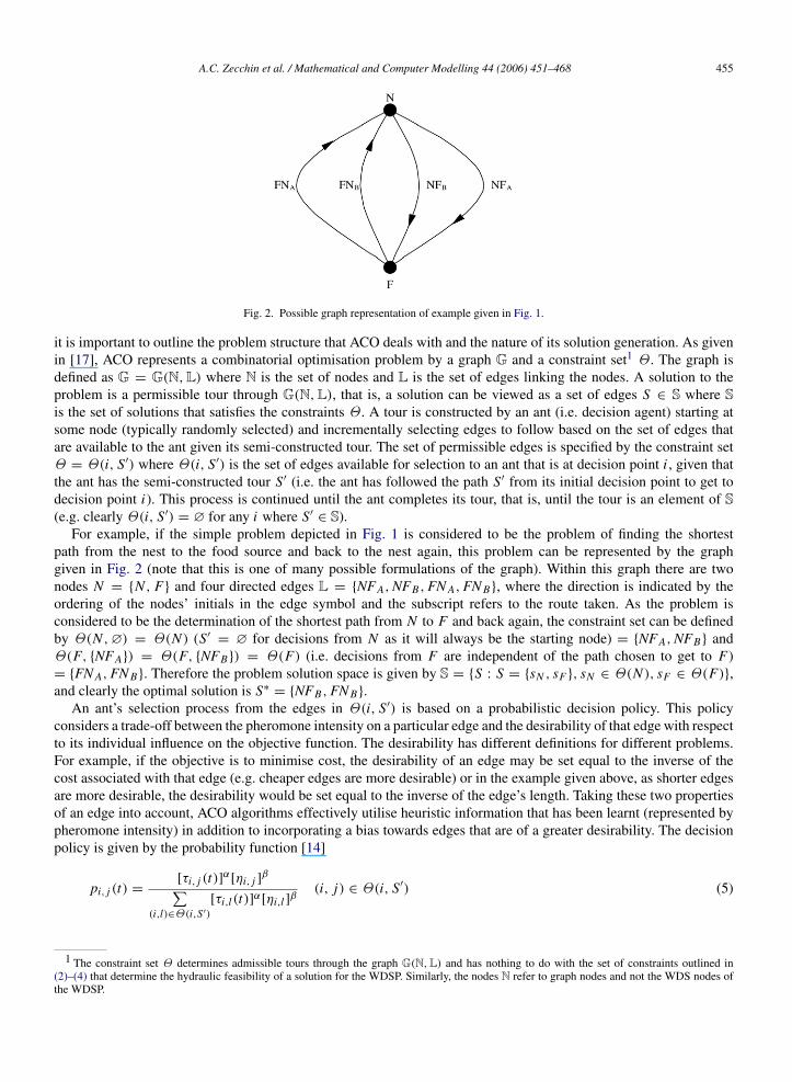
Fig. 2. Possible graph representation of example given in Fig. 1.

it is important to outline the problem structure that ACO deals with and the nature of its solution generation. As givenin [17], ACO represents a combinatorial optimisation problem by a graph G and a constraint set1 Θ . The graph isdefined as G = G(N, L) where N is the set of nodes and L is the set of edges linking the nodes. A solution to theproblem is a permissible tour through G(N, L), that is, a solution can be viewed as a set of edges S ∈ S where Sis the set of solutions that satisfies the constraints Θ . A tour is constructed by an ant (i.e. decision agent) starting atsome node (typically randomly selected) and incrementally selecting edges to follow based on the set of edges thatare available to the ant given its semi-constructed tour. The set of permissible edges is specified by the constraint setΘ = Θ(i, S′) where Θ(i, S′) is the set of edges available for selection to an ant that is at decision point i , given thatthe ant has the semi-constructed tour S′ (i.e. the ant has followed the path S′ from its initial decision point to get todecision point i). This process is continued until the ant completes its tour, that is, until the tour is an element of S(e.g. clearly Θ(i, S′) = ∅ for any i where S′

∈ S).For example, if the simple problem depicted in Fig. 1 is considered to be the problem of finding the shortest

path from the nest to the food source and back to the nest again, this problem can be represented by the graphgiven in Fig. 2 (note that this is one of many possible formulations of the graph). Within this graph there are twonodes N = N , F and four directed edges L = NFA, NFB, FN A, FN B, where the direction is indicated by theordering of the nodes’ initials in the edge symbol and the subscript refers to the route taken. As the problem isconsidered to be the determination of the shortest path from N to F and back again, the constraint set can be definedby Θ(N , ∅) = Θ(N ) (S′

= ∅ for decisions from N as it will always be the starting node) = NFA, NFB andΘ(F, NFA) = Θ(F, NFB) = Θ(F) (i.e. decisions from F are independent of the path chosen to get to F)= FN A, FN B. Therefore the problem solution space is given by S = S : S = sN , sF , sN ∈ Θ(N ), sF ∈ Θ(F),and clearly the optimal solution is S∗

= NFB, FN B.An ant’s selection process from the edges in Θ(i, S′) is based on a probabilistic decision policy. This policy

considers a trade-off between the pheromone intensity on a particular edge and the desirability of that edge with respectto its individual influence on the objective function. The desirability has different definitions for different problems.For example, if the objective is to minimise cost, the desirability of an edge may be set equal to the inverse of thecost associated with that edge (e.g. cheaper edges are more desirable) or in the example given above, as shorter edgesare more desirable, the desirability would be set equal to the inverse of the edge’s length. Taking these two propertiesof an edge into account, ACO algorithms effectively utilise heuristic information that has been learnt (represented bypheromone intensity) in addition to incorporating a bias towards edges that are of a greater desirability. The decisionpolicy is given by the probability function [14]

pi, j (t) =[τi, j (t)]α[ηi, j ]

β∑(i,l)∈Θ(i,S′)

[τi,l(t)]α[ηi,l ]β

(i, j) ∈ Θ(i, S′) (5)

1 The constraint set Θ determines admissible tours through the graph G(N,L) and has nothing to do with the set of constraints outlined in(2)–(4) that determine the hydraulic feasibility of a solution for the WDSP. Similarly, the nodes N refer to graph nodes and not the WDS nodes ofthe WDSP.

456 A.C. Zecchin et al. / Mathematical and Computer Modelling 44 (2006) 451–468

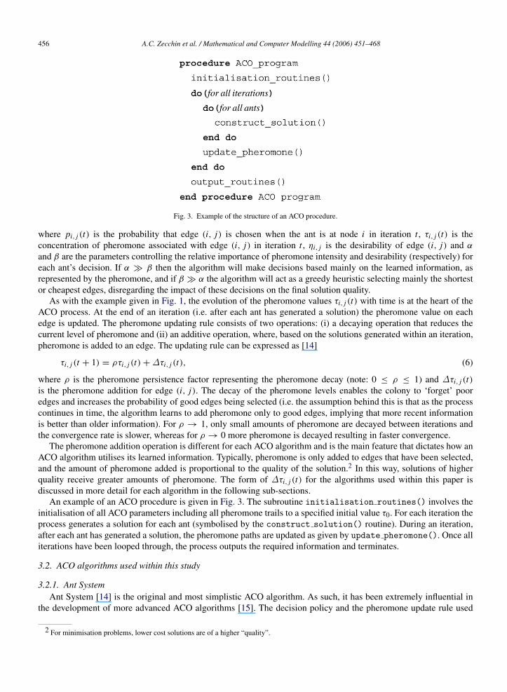
Fig. 3. Example of the structure of an ACO procedure.

where pi, j (t) is the probability that edge (i, j) is chosen when the ant is at node i in iteration t , τi, j (t) is theconcentration of pheromone associated with edge (i, j) in iteration t , ηi, j is the desirability of edge (i, j) and α

and β are the parameters controlling the relative importance of pheromone intensity and desirability (respectively) foreach ant’s decision. If α β then the algorithm will make decisions based mainly on the learned information, asrepresented by the pheromone, and if β α the algorithm will act as a greedy heuristic selecting mainly the shortestor cheapest edges, disregarding the impact of these decisions on the final solution quality.

As with the example given in Fig. 1, the evolution of the pheromone values τi, j (t) with time is at the heart of theACO process. At the end of an iteration (i.e. after each ant has generated a solution) the pheromone value on eachedge is updated. The pheromone updating rule consists of two operations: (i) a decaying operation that reduces thecurrent level of pheromone and (ii) an additive operation, where, based on the solutions generated within an iteration,pheromone is added to an edge. The updating rule can be expressed as [14]

τi, j (t + 1) = ρτi, j (t) + ∆τi, j (t), (6)

where ρ is the pheromone persistence factor representing the pheromone decay (note: 0 ≤ ρ ≤ 1) and ∆τi, j (t)is the pheromone addition for edge (i, j). The decay of the pheromone levels enables the colony to ‘forget’ pooredges and increases the probability of good edges being selected (i.e. the assumption behind this is that as the processcontinues in time, the algorithm learns to add pheromone only to good edges, implying that more recent informationis better than older information). For ρ → 1, only small amounts of pheromone are decayed between iterations andthe convergence rate is slower, whereas for ρ → 0 more pheromone is decayed resulting in faster convergence.

The pheromone addition operation is different for each ACO algorithm and is the main feature that dictates how anACO algorithm utilises its learned information. Typically, pheromone is only added to edges that have been selected,and the amount of pheromone added is proportional to the quality of the solution.2 In this way, solutions of higherquality receive greater amounts of pheromone. The form of ∆τi, j (t) for the algorithms used within this paper isdiscussed in more detail for each algorithm in the following sub-sections.

An example of an ACO procedure is given in Fig. 3. The subroutine initialisation routines() involves theinitialisation of all ACO parameters including all pheromone trails to a specified initial value τ0. For each iteration theprocess generates a solution for each ant (symbolised by the construct solution() routine). During an iteration,after each ant has generated a solution, the pheromone paths are updated as given by update pheromone(). Once alliterations have been looped through, the process outputs the required information and terminates.

3.2. ACO algorithms used within this study

3.2.1. Ant SystemAnt System [14] is the original and most simplistic ACO algorithm. As such, it has been extremely influential in

the development of more advanced ACO algorithms [15]. The decision policy and the pheromone update rule used

2 For minimisation problems, lower cost solutions are of a higher “quality”.

A.C. Zecchin et al. / Mathematical and Computer Modelling 44 (2006) 451–468 457

within AS are given by (5) and (6), respectively. For AS, each ant adds pheromone to all edges it has selected andconsequently the pheromone addition received by each edge (i, j) ∈ L is given by [14]

∆τi, j (t) =

m∑k=1

∆τ ki, j (t), (7)

where m is the number of ants and ∆τ ki, j (t) is the additional pheromone laid on edge (i, j) by the kth ant at the end

of iteration t . The individual pheromone addition contributed by each ant is given by [14]

∆τ ki, j (t) =

Q

f (Sk(t))if (i, j) ∈ Sk(t)

0 otherwise,(8)

where Q is the pheromone addition factor (a constant), Sk(t) is the set of edges selected by ant k in iteration t andf (·) is the objective function. From (8) it is clear that ants only add pheromone to the edges that they select andthat solutions of better quality (e.g. solutions with lower f (·) values, as the problem is assumed to be a minimisationproblem) are rewarded with greater pheromone additions.

3.2.2. Max-Min Ant SystemPremature convergence to sub-optimal solutions is an issue that can be experienced by all HDNs, especially those

that have a greater emphasis on exploitation. To overcome this problem, the Max-Min Ant System (MMAS) wasdeveloped by Stutzle and Hoos [16]. The basis of MMAS is to provide dynamically evolving bounds on the pheromonetrail intensities such that the pheromone intensity on all paths is always within a specified limit of the path with thegreatest pheromone intensity. As a result all paths will always have a non-trivial probability of being selected and thuswider exploration of the search space is encouraged.

MMAS uses upper and lower bounds to ensure pheromone intensities lie within a given range, that is τmin(t) ≤

τi, j (t) ≤ τmax(t). The upper bound τmax(t) is given by3 [16]

τmax(t) =1

1 − ρ

Q

f (Sgb(t − 1))(9)

where Sgb(t) is the global best path found up to iteration t , and the lower bound τmin(t) is given by [16]

τmin(t) =τmax(t)

(1 − n

√pbest

)(NOavg − 1) n

√pbest

(10)

where pbest is the probability that Sgb(t) will be selected by any ant in iteration t given that all non-global best edgeshave a pheromone level of τmin(t) and all global-best edges have a pheromone level of τmax(t), n is the number ofdecision points and NOavg is the average number of edges at each decision point. Within MMAS, the pheromone pathsare initialised to an arbitrarily high value such that in the second iteration the paths are set to τmax(t).

Theoretical justifications of the bounds are given in [16] but here it is sufficient to say that τmax(t) is the theoreticalasymptotic maximum pheromone level that an edge repeatedly receiving pheromone additions of Q/ f (Sgb(t)) canachieve and τmin(t) is an approximation to the pheromone level such that in the limit as t → ∞, the probability thatan ant selects Sgb(t) is pbest. An analysis of (10) shows that lower values of pbest indicate tighter pheromone bounds,that is τmin(t) → τmax(t) as pbest → 0.

As the bounds serve to encourage exploration, to provide an emphasis on exploitation, MMAS updates the iterationbest ant’s path and periodically the global best path at the end of an iteration to ensure that good information is beingretained and reinforced. The updating scheme is as in (6) where ∆τi, j (t) is given by

∆τi, j (t) = ∆τ ibi, j (t) + ∆τ

gbi, j (t), (11)

3 [16] Omit Q from their formulation, but for the sake of consistency with the adopted formulation of AS, it is included in this study.

458 A.C. Zecchin et al. / Mathematical and Computer Modelling 44 (2006) 451–468

where the addition from the iteration best ant ∆τ ibi, j (t) is given by

∆τ ibi, j (t) =

Q

f (Sib(t))if (i, j) ∈ Sib(t)

0 otherwise(12)

where Sib(t) is the iteration best path found in iteration t . The pheromone addition from the global best ant ∆τgbi, j (t)

is given by

∆τgbi, j (t) =

1

f (Sgb(t))if (i, j) ∈ Sgb(t) and t = p fglobal where p ∈ N

0 otherwise(13)

where fglobal is the frequency of the global best pheromone updating and N is the set of natural numbers. MMAS alsoutilises another mechanism known as pheromone trail smoothing (PTS). This reduces the relative difference betweenthe pheromone intensities, and further encourages exploration. The PTS mechanism is given by [16]

τ ∗

i, j (t) = τi, j (t) + δ(τmax(t) − τi, j (t)), (14)

where 0 ≤ δ ≤ 1 is the PTS coefficient, and τ ∗

i, j (t) is the pheromone intensity after the smoothing. If δ = 0 the PTSmechanism has no effect, whereas if δ = 1 all pheromone paths are scaled up to τmax(t).

4. Application of ant colony optimisation to water distribution system optimisation

4.1. Transformation of constrained problem

The WDSP is a constrained optimisation problem. ACO, as all HDNs, is unable to deal directly with constrainedoptimisation problems as, within its solution generation, it cannot adhere to constraints that separate feasible regionsof a search space from infeasible regions. The standard technique to convert constrained problems to unconstrainedproblems is to use a penalty function. HDNs direct their search solely based on information provided by theobjective function. To guide the search away from the infeasible region and towards the feasible region, a penaltyfunction increases the cost of infeasible solutions such that they are considered to be undesirable. The unconstrainedoptimisation problem for the WDSP takes the form of minimising the sum of the real cost plus the penalty cost, thatis

min NC(Ω) = C(Ω) + PC(Ω) (15)

where NC(Ω) is the network cost for design Ω , C(Ω) is the material and installation cost of Ω (i.e. the objective ofthe constrained problem) and PC(Ω) is the penalty cost incurred by Ω . Within this study, PC(Ω) was taken to beproportional to the maximum nodal pressure deficit induced by Ω as in [12]. That is

PC(Ω) =

0 H j

i (Ω) ≥ H ji ∀i = 1, . . . , Nnode ∀ j = 1, . . . , Npattern

maxi=1,...,Nnode

j=1,...,Npattern

H j

i − H ji (Ω)

.PEN otherwise (16)

where PEN is the penalty factor (constant) with units of dollars per meter of pressure violation (note, the set ofheads H j

i (Ω) : i = 1, . . . , Nnode, j = 1, . . . , Npattern is calculated by a hydraulic solver). The parameter PENis a user-defined parameter and appropriate values of PEN are different for each case study. To reduce calibrationalrequirements, a semi-deterministic expression for PEN derived in [13] is used, that is

PEN =[C(Ωmax) − C(Ωmin)]

d(17)

where Ωmax and Ωmin are the maximum and minimum material cost network designs, respectively, and d is a userselected pressure deficit. The value of PEN ensures that all networks with a pressure violation greater than or equal tod (an extremely small value) are made more expensive than the maximum feasible network cost.

A.C. Zecchin et al. / Mathematical and Computer Modelling 44 (2006) 451–468 459

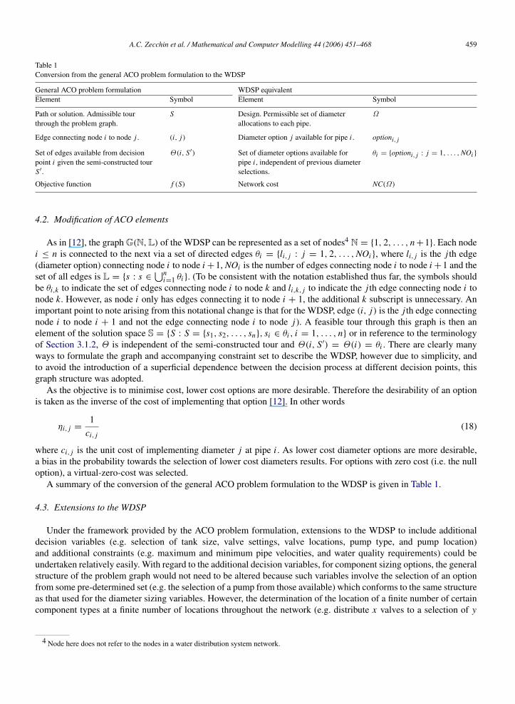
Table 1Conversion from the general ACO problem formulation to the WDSP

General ACO problem formulation WDSP equivalentElement Symbol Element Symbol

Path or solution. Admissible tourthrough the problem graph.

S Design. Permissible set of diameterallocations to each pipe.

Ω

Edge connecting node i to node j . (i, j) Diameter option j available for pipe i . optioni, j

Set of edges available from decisionpoint i given the semi-constructed tourS′.

Θ(i, S′) Set of diameter options available forpipe i , independent of previous diameterselections.

θi = optioni, j : j = 1, . . . , NOi

Objective function f (S) Network cost NC(Ω)

4.2. Modification of ACO elements

As in [12], the graph G(N, L) of the WDSP can be represented as a set of nodes4 N = 1, 2, . . . , n +1. Each nodei ≤ n is connected to the next via a set of directed edges θi = li, j : j = 1, 2, . . . , NOi , where li, j is the j th edge(diameter option) connecting node i to node i +1, NOi is the number of edges connecting node i to node i +1 and theset of all edges is L = s : s ∈

⋃ni=1 θi . (To be consistent with the notation established thus far, the symbols should

be θi,k to indicate the set of edges connecting node i to node k and li,k, j to indicate the j th edge connecting node i tonode k. However, as node i only has edges connecting it to node i + 1, the additional k subscript is unnecessary. Animportant point to note arising from this notational change is that for the WDSP, edge (i, j) is the j th edge connectingnode i to node i + 1 and not the edge connecting node i to node j). A feasible tour through this graph is then anelement of the solution space S = S : S = s1, s2, . . . , sn, si ∈ θi , i = 1, . . . , n or in reference to the terminologyof Section 3.1.2, Θ is independent of the semi-constructed tour and Θ(i, S′) = Θ(i) = θi . There are clearly manyways to formulate the graph and accompanying constraint set to describe the WDSP, however due to simplicity, andto avoid the introduction of a superficial dependence between the decision process at different decision points, thisgraph structure was adopted.

As the objective is to minimise cost, lower cost options are more desirable. Therefore the desirability of an optionis taken as the inverse of the cost of implementing that option [12]. In other words

ηi, j =1

ci, j(18)

where ci, j is the unit cost of implementing diameter j at pipe i . As lower cost diameter options are more desirable,a bias in the probability towards the selection of lower cost diameters results. For options with zero cost (i.e. the nulloption), a virtual-zero-cost was selected.

A summary of the conversion of the general ACO problem formulation to the WDSP is given in Table 1.

4.3. Extensions to the WDSP

Under the framework provided by the ACO problem formulation, extensions to the WDSP to include additionaldecision variables (e.g. selection of tank size, valve settings, valve locations, pump type, and pump location)and additional constraints (e.g. maximum and minimum pipe velocities, and water quality requirements) could beundertaken relatively easily. With regard to the additional decision variables, for component sizing options, the generalstructure of the problem graph would not need to be altered because such variables involve the selection of an optionfrom some pre-determined set (e.g. the selection of a pump from those available) which conforms to the same structureas that used for the diameter sizing variables. However, the determination of the location of a finite number of certaincomponent types at a finite number of locations throughout the network (e.g. distribute x valves to a selection of y

4 Node here does not refer to the nodes in a water distribution system network.

460 A.C. Zecchin et al. / Mathematical and Computer Modelling 44 (2006) 451–468

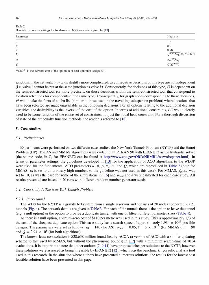
Table 2Heuristic parameter settings for fundamental ACO parameters given by [13]

Parameter Heuristic

α 1.0β 0.5ρ 0.98τ0

√nNOavg.Q/NC(Ω∗)

m n√

NOavg

Q C(Ωmax)

NC(Ω∗) is the network cost of the optimum or near optimum design Ω∗.

junctions in the network, y > x) is slightly more complicated, as consecutive decisions of this type are not independent(i.e. valve i cannot be put at the same junction as valve k). Consequently, for decisions of this type, Θ is dependent onthe semi-constructed tour (or more precisely, on those decisions within the semi-constructed tour that correspond tolocation selections for components of the same type). Consequently, for graph nodes corresponding to these decisions,Θ would take the form of a tabu list (similar to those used in the travelling salesperson problem) where locations thathave been selected are made unavailable in the following decisions. For all options relating to the additional decisionvariables, the desirability is the inverse of the cost of the option. In terms of additional constraints, PC would clearlyneed to be some function of the entire set of constraints, not just the nodal head constraint. For a thorough discussionof state of the art penalty function methods, the reader is referred to [18].

5. Case studies

5.1. Preliminaries

Experiments were performed on two different case studies, the New York Tunnels Problem (NYTP) and the HanoiProblem (HP). The AS and MMAS algorithms were coded in FORTRAN 90 with EPANET2 as the hydraulic solver(the source code, in C, for EPANET2 can be found at http://www.epa.gov/ORD/NRMRL/wswrd/epanet.html). Interms of parameter settings, the guidelines developed in [13] for the application of ACO algorithms to the WDSPwere used for the fundamental ACO parameters α, β, ρ, τ0, m, and Q, which are reproduced in Table 2 (note forMMAS, τ0 is set to an arbitrary high number, so the guideline was not used in this case). For MMAS, fglobal wasset to 10, as was the case for some of the simulations in [16] and pbest and δ were calibrated for each case study. Allresults presented are based on 20 runs with different random number generator seeds.

5.2. Case study 1: The New York Tunnels Problem

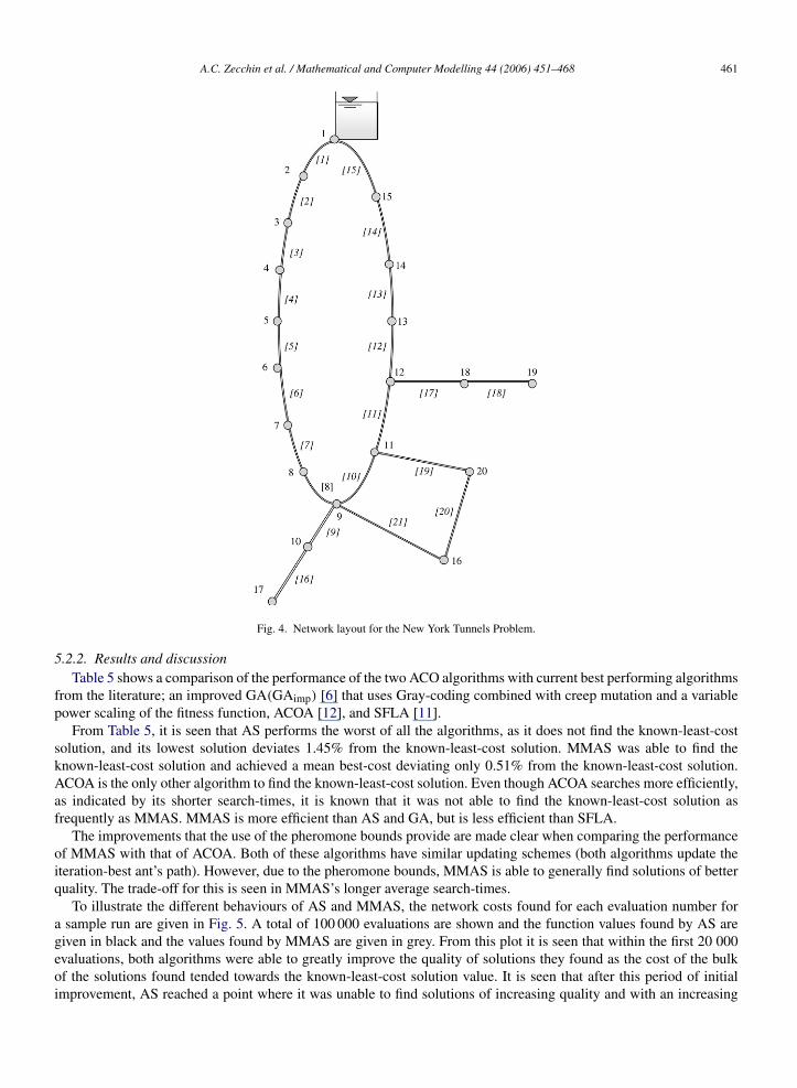
5.2.1. BackgroundThe WDS for the NYTP is a gravity fed system from a single reservoir and consists of 20 nodes connected via 21

tunnels (Fig. 4). The network details are given in Table 3. For each of the tunnels there is the option to leave the tunnel(e.g. a null option) or the option to provide a duplicate tunnel with one of fifteen different diameter sizes (Table 4).

As there is a null option, a virtual-zero-cost of $110 per metre was used in this study. This is approximately 1/3 ofthe cost of the cheapest duplicate option. This case study has a search space of approximately 1.934 × 1025 possibledesigns. The parameters were set as follows: τ0 = 140 (for AS), pbest = 0.05, δ = 5 × 10−5 (for MMAS), m = 90and Q = 2.94 × 108 (for both algorithms).

The known-least-cost solution is $38.638 million found first by ACOA (a version of ACO with a similar updatingscheme to that used by MMAS, but without the pheromone bounds) in [12] with a minimum search-time of 7014evaluations. It is important to note that other authors [7–9,11] have proposed cheaper solutions to the NYTP, howeverthese solutions were assessed as being infeasible by EPANET2 [12], which was the benchmark hydraulic analysis toolused in this research. In the situation where authors have presented numerous solutions, the results for the lowest costfeasible solution have been presented in this paper.

A.C. Zecchin et al. / Mathematical and Computer Modelling 44 (2006) 451–468 461

Fig. 4. Network layout for the New York Tunnels Problem.

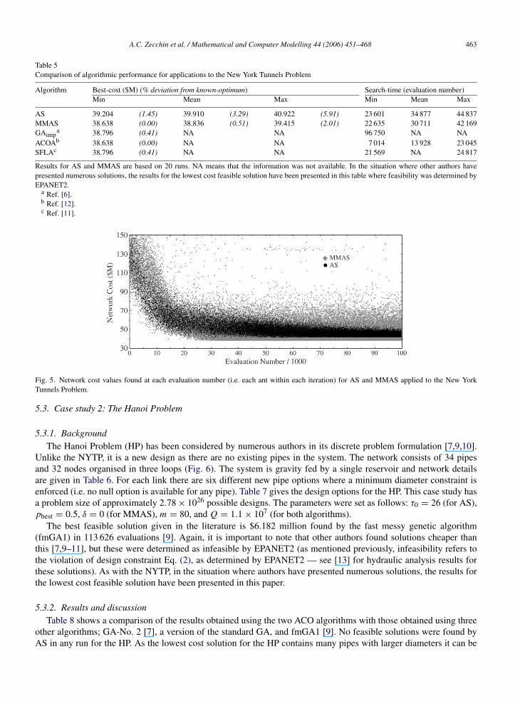
5.2.2. Results and discussionTable 5 shows a comparison of the performance of the two ACO algorithms with current best performing algorithms

from the literature; an improved GA(GAimp) [6] that uses Gray-coding combined with creep mutation and a variablepower scaling of the fitness function, ACOA [12], and SFLA [11].

From Table 5, it is seen that AS performs the worst of all the algorithms, as it does not find the known-least-costsolution, and its lowest solution deviates 1.45% from the known-least-cost solution. MMAS was able to find theknown-least-cost solution and achieved a mean best-cost deviating only 0.51% from the known-least-cost solution.ACOA is the only other algorithm to find the known-least-cost solution. Even though ACOA searches more efficiently,as indicated by its shorter search-times, it is known that it was not able to find the known-least-cost solution asfrequently as MMAS. MMAS is more efficient than AS and GA, but is less efficient than SFLA.

The improvements that the use of the pheromone bounds provide are made clear when comparing the performanceof MMAS with that of ACOA. Both of these algorithms have similar updating schemes (both algorithms update theiteration-best ant’s path). However, due to the pheromone bounds, MMAS is able to generally find solutions of betterquality. The trade-off for this is seen in MMAS’s longer average search-times.

To illustrate the different behaviours of AS and MMAS, the network costs found for each evaluation number fora sample run are given in Fig. 5. A total of 100 000 evaluations are shown and the function values found by AS aregiven in black and the values found by MMAS are given in grey. From this plot it is seen that within the first 20 000evaluations, both algorithms were able to greatly improve the quality of solutions they found as the cost of the bulkof the solutions found tended towards the known-least-cost solution value. It is seen that after this period of initialimprovement, AS reached a point where it was unable to find solutions of increasing quality and with an increasing

462 A.C. Zecchin et al. / Mathematical and Computer Modelling 44 (2006) 451–468

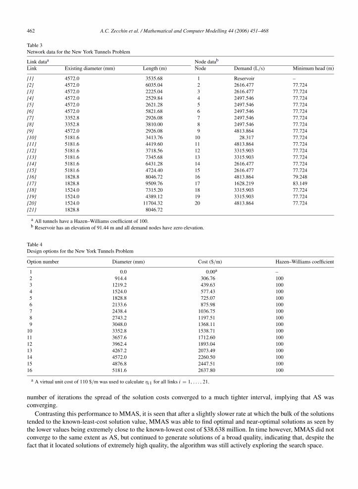
Table 3Network data for the New York Tunnels Problem

Link dataa Node datab

Link Existing diameter (mm) Length (m) Node Demand (L/s) Minimum head (m)

[1] 4572.0 3535.68 1 Reservoir –[2] 4572.0 6035.04 2 2616.477 77.724[3] 4572.0 2225.04 3 2616.477 77.724[4] 4572.0 2529.84 4 2497.546 77.724[5] 4572.0 2621.28 5 2497.546 77.724[6] 4572.0 5821.68 6 2497.546 77.724[7] 3352.8 2926.08 7 2497.546 77.724[8] 3352.8 3810.00 8 2497.546 77.724[9] 4572.0 2926.08 9 4813.864 77.724[10] 5181.6 3413.76 10 28.317 77.724[11] 5181.6 4419.60 11 4813.864 77.724[12] 5181.6 3718.56 12 3315.903 77.724[13] 5181.6 7345.68 13 3315.903 77.724[14] 5181.6 6431.28 14 2616.477 77.724[15] 5181.6 4724.40 15 2616.477 77.724[16] 1828.8 8046.72 16 4813.864 79.248[17] 1828.8 9509.76 17 1628.219 83.149[18] 1524.0 7315.20 18 3315.903 77.724[19] 1524.0 4389.12 19 3315.903 77.724[20] 1524.0 11704.32 20 4813.864 77.724[21] 1828.8 8046.72

a All tunnels have a Hazen–Williams coefficient of 100.b Reservoir has an elevation of 91.44 m and all demand nodes have zero elevation.

Table 4Design options for the New York Tunnels Problem

Option number Diameter (mm) Cost ($/m) Hazen–Williams coefficient

1 0.0 0.00a –2 914.4 306.76 1003 1219.2 439.63 1004 1524.0 577.43 1005 1828.8 725.07 1006 2133.6 875.98 1007 2438.4 1036.75 1008 2743.2 1197.51 1009 3048.0 1368.11 100

10 3352.8 1538.71 10011 3657.6 1712.60 10012 3962.4 1893.04 10013 4267.2 2073.49 10014 4572.0 2260.50 10015 4876.8 2447.51 10016 5181.6 2637.80 100

a A virtual unit cost of 110 $/m was used to calculate ηi1 for all links i = 1, . . . , 21.

number of iterations the spread of the solution costs converged to a much tighter interval, implying that AS wasconverging.

Contrasting this performance to MMAS, it is seen that after a slightly slower rate at which the bulk of the solutionstended to the known-least-cost solution value, MMAS was able to find optimal and near-optimal solutions as seen bythe lower values being extremely close to the known-lowest cost of $38.638 million. In time however, MMAS did notconverge to the same extent as AS, but continued to generate solutions of a broad quality, indicating that, despite thefact that it located solutions of extremely high quality, the algorithm was still actively exploring the search space.

A.C. Zecchin et al. / Mathematical and Computer Modelling 44 (2006) 451–468 463

Table 5Comparison of algorithmic performance for applications to the New York Tunnels Problem

Algorithm Best-cost ($M) (% deviation from known-optimum) Search-time (evaluation number)Min Mean Max Min Mean Max

AS 39.204 (1.45) 39.910 (3.29) 40.922 (5.91) 23 601 34 877 44 837MMAS 38.638 (0.00) 38.836 (0.51) 39.415 (2.01) 22 635 30 711 42 169GAimp

a 38.796 (0.41) NA NA 96 750 NA NAACOAb 38.638 (0.00) NA NA 7 014 13 928 23 045SFLAc 38.796 (0.41) NA NA 21 569 NA 24 817

Results for AS and MMAS are based on 20 runs. NA means that the information was not available. In the situation where other authors havepresented numerous solutions, the results for the lowest cost feasible solution have been presented in this table where feasibility was determined byEPANET2.

a Ref. [6].b Ref. [12].c Ref. [11].

Fig. 5. Network cost values found at each evaluation number (i.e. each ant within each iteration) for AS and MMAS applied to the New YorkTunnels Problem.

5.3. Case study 2: The Hanoi Problem

5.3.1. BackgroundThe Hanoi Problem (HP) has been considered by numerous authors in its discrete problem formulation [7,9,10].

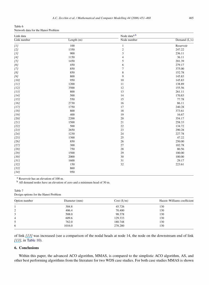
Unlike the NYTP, it is a new design as there are no existing pipes in the system. The network consists of 34 pipesand 32 nodes organised in three loops (Fig. 6). The system is gravity fed by a single reservoir and network detailsare given in Table 6. For each link there are six different new pipe options where a minimum diameter constraint isenforced (i.e. no null option is available for any pipe). Table 7 gives the design options for the HP. This case study hasa problem size of approximately 2.78 × 1026 possible designs. The parameters were set as follows: τ0 = 26 (for AS),pbest = 0.5, δ = 0 (for MMAS), m = 80, and Q = 1.1 × 107 (for both algorithms).

The best feasible solution given in the literature is $6.182 million found by the fast messy genetic algorithm(fmGA1) in 113 626 evaluations [9]. Again, it is important to note that other authors found solutions cheaper thanthis [7,9–11], but these were determined as infeasible by EPANET2 (as mentioned previously, infeasibility refers tothe violation of design constraint Eq. (2), as determined by EPANET2 — see [13] for hydraulic analysis results forthese solutions). As with the NYTP, in the situation where authors have presented numerous solutions, the results forthe lowest cost feasible solution have been presented in this paper.

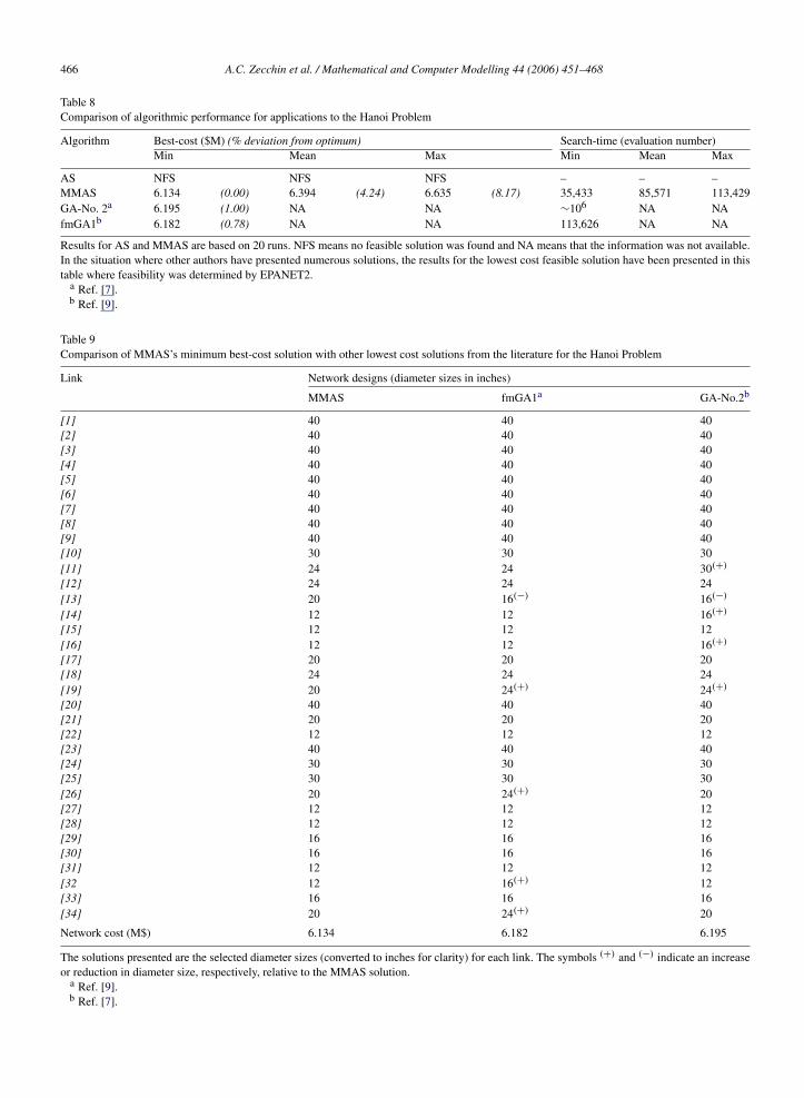
5.3.2. Results and discussionTable 8 shows a comparison of the results obtained using the two ACO algorithms with those obtained using three

other algorithms; GA-No. 2 [7], a version of the standard GA, and fmGA1 [9]. No feasible solutions were found byAS in any run for the HP. As the lowest cost solution for the HP contains many pipes with larger diameters it can be

464 A.C. Zecchin et al. / Mathematical and Computer Modelling 44 (2006) 451–468

Fig. 6. Network layout for the Hanoi Problem.

deduced that the problem has a small feasible region, thus explaining AS’s poor performance. Other authors have alsoreported on the difficulty associated with this problem [11].

MMAS was found to be the best performing algorithm for this case study as it was able to find a new lowest costsolution, 0.78% less than the previous lowest cost solution found by fmGA1 [9]. MMAS also achieved the lowestmean best-cost (deviating 4.24% from the new best solution) but also had the longest search-times. The performanceof MMAS compared to that of AS is a result of its ability to explore the search space more widely for a longer period oftime, resulting from its non-convergence mechanisms, but still having its search guided by only the best information,resulting from its elitist updating scheme.

A comparison of the lowest cost solution found by MMAS along with the solutions found by fmGA1 and GA-No.2is given in Table 9. It can be seen that both the fmGA1 and GA-No.2 solutions differ from the MMAS solution by fivelinks, which corresponds to an 85% similarity between the solutions. Of these five different links, four pipes of boththe fmGA1 and GA-No.2 solutions have larger diameters than the solution found by MMAS, and only the diameterof link [13] is larger for the solution found by the MMAS algorithm compared with those found by the GAs. Aninteresting point to note is that the first 18 links of the MMAS solution are identical to those of the fmGA1 solution(except link [13]) and the last 15 links are identical to those of the GA-No.2 solution. These similarities correspondto the right-most loop of the MMAS solution being the same as the right-most loop of the fmGA1 solution (except forlink [19]) and the left-most and centre loop being the same for the MMAS and GA-No.2 solutions (see Fig. 6).

Nodal heads for selected nodes and link flows for selected links are given in Tables 10 and 11, respectively.Considering the three main links from the source feeding the network (links [3], [19], and [20]), it is seen thatthe MMAS solution increases the flow to the right-most arc through [3] and reduces the flow up the right-centre mainthrough [19]. The increased flow through the right-most arc explains the need for the increase in the diameter size atlink [13] in the MMAS solution. The extra flow in the right-most arc is used to provide a greater flow to nodes alongthe top main (as illustrated by the larger flow rate in links [13] and [14] of the MMAS solution in Table 11) and soto reduce frictional losses (to maintain an adequate pressure head and hence provide a feasible solution) the diameter

A.C. Zecchin et al. / Mathematical and Computer Modelling 44 (2006) 451–468 465

Table 6Network data for the Hanoi Problem

Link data Node dataa,b

Link number Length (m) Node number Demand (L/s)

[1] 100 1 Reservoir[2] 1350 2 247.22[3] 900 3 236.11[4] 1150 4 36.11[5] 1450 5 201.39[6] 450 6 279.17[7] 850 7 375.00[8] 850 8 152.78[9] 800 9 145.83[10] 950 10 145.83[11] 1200 11 138.89[12] 3500 12 155.56[13] 800 13 261.11[14] 500 14 170.83[15] 550 15 77.78[16] 2730 16 86.11[17] 1750 17 240.28[18] 800 18 373.61[19] 400 19 16.67[20] 2200 20 354.17[21] 1500 21 258.33[22] 500 22 134.72[23] 2650 23 290.28[24] 1230 24 227.78[25] 1300 25 47.22[26] 850 26 250.00[27] 300 27 102.78[28] 750 28 80.56[29] 1500 29 100.00[30] 2000 30 100.00[31] 1600 31 29.17[32] 150 32 223.61[33] 860[34] 950

a Reservoir has an elevation of 100 m.b All demand nodes have an elevation of zero and a minimum head of 30 m.

Table 7Design options for the Hanoi Problem

Option number Diameter (mm) Cost ($/m) Hazen–Williams coefficient

1 304.8 45.726 1302 406.4 70.400 1303 508.0 98.378 1304 609.6 129.333 1305 762.0 180.748 1306 1016.0 278.280 130

of link [13] was increased (see a comparison of the nodal heads at node 14, the node on the downstream end of link[13], in Table 10).

6. Conclusions

Within this paper, the advanced ACO algorithm, MMAS, is compared to the simplistic ACO algorithm, AS, andother best performing algorithms from the literature for two WDS case studies. For both case studies MMAS is shown

466 A.C. Zecchin et al. / Mathematical and Computer Modelling 44 (2006) 451–468

Table 8Comparison of algorithmic performance for applications to the Hanoi Problem

Algorithm Best-cost ($M) (% deviation from optimum) Search-time (evaluation number)Min Mean Max Min Mean Max

AS NFS NFS NFS – – –MMAS 6.134 (0.00) 6.394 (4.24) 6.635 (8.17) 35,433 85,571 113,429GA-No. 2a 6.195 (1.00) NA NA ∼106 NA NAfmGA1b 6.182 (0.78) NA NA 113,626 NA NA

Results for AS and MMAS are based on 20 runs. NFS means no feasible solution was found and NA means that the information was not available.In the situation where other authors have presented numerous solutions, the results for the lowest cost feasible solution have been presented in thistable where feasibility was determined by EPANET2.

a Ref. [7].b Ref. [9].

Table 9Comparison of MMAS’s minimum best-cost solution with other lowest cost solutions from the literature for the Hanoi Problem

Link Network designs (diameter sizes in inches)

MMAS fmGA1a GA-No.2b

[1] 40 40 40[2] 40 40 40[3] 40 40 40[4] 40 40 40[5] 40 40 40[6] 40 40 40[7] 40 40 40[8] 40 40 40[9] 40 40 40[10] 30 30 30[11] 24 24 30(+)

[12] 24 24 24[13] 20 16(−) 16(−)

[14] 12 12 16(+)

[15] 12 12 12[16] 12 12 16(+)

[17] 20 20 20[18] 24 24 24[19] 20 24(+) 24(+)

[20] 40 40 40[21] 20 20 20[22] 12 12 12[23] 40 40 40[24] 30 30 30[25] 30 30 30[26] 20 24(+) 20[27] 12 12 12[28] 12 12 12[29] 16 16 16[30] 16 16 16[31] 12 12 12[32 12 16(+) 12[33] 16 16 16[34] 20 24(+) 20

Network cost (M$) 6.134 6.182 6.195

The solutions presented are the selected diameter sizes (converted to inches for clarity) for each link. The symbols (+) and (−) indicate an increaseor reduction in diameter size, respectively, relative to the MMAS solution.

a Ref. [9].b Ref. [7].

A.C. Zecchin et al. / Mathematical and Computer Modelling 44 (2006) 451–468 467

Table 10Pressure excess (m) for critical nodes for designs (solutions) presented in Table 9

Node Pressure excess (m)

MMAS fmGA1a GA-No.2b

13 0.940 1.756 4.18414 7.247 4.275(−) 4.774(−)

15 2.952 2.072(−) 4.31316 2.230 2.046(−) 4.31326 2.659 3.590 3.65627 1.705 1.998 3.10029 1.361 2.294 1.84430 0.419 1.846 0.97331 0.895 1.994 1.46532 2.166 3.496 2.764

A critical node here is defined as one where one of the three designs has a pressure excess less than 5 m above the minimum allowable pressurehead. Nodes with lower pressure heads than those for the MMAS solution are marked with (−). Hydraulic analysis was performed using EPANET2.

a Ref. [9].b Ref. [7].

Table 11Flow rates (L/s) in main links distributing flow from source and links where the MMAS design has differing diameter sizes from the other solutionsin Table 9

Link Flow rate (L/s)

MMAS fmGA1b GA-No.2c

[3]a 2184.39 2147.45(−) 2140.28(−)

[11] 416.76 416.76 416.76[13] 292.86 255.93(−) 248.76(−)

[14] 121.99 85.06(−) 77.89(−)

[16] 73.40 87.61 135.54[19]a 704.10 718.31 766.24[20]a 2167.63 2190.35 2149.59(−)

[26] 321.39 344.11 303.36(−)

[32] 71.32 80.80 72.52[34] 324.15 333.63 325.35

Links with flow less than the MMAS design are marked (−). Hydraulic analysis was performed using EPANET2.a Main links leading from source (i.e. the reservoir at node 1).b Ref. [9].c Ref. [7].

to outperform AS. The ease at which the water distribution system problem can be translated into the ACO problemparadigm combined with the excellent performance of MMAS illustrate that ACO is a well suited algorithm for thisproblem.

Within the first case study, the New York Tunnels Problem (NYTP), MMAS found the known-least-cost solutionand provided the best performance found within the literature for this case study5 (MMAS achieved a mean objectivefunction deviation of 0.51% from the known-least-cost solution value). AS was unable to find the known-least-costsolution for any runs. For the second case study, the Hanoi Problem (HP), AS performed worse than all the algorithmsunder consideration, as it was unable to find any feasible solutions. MMAS, again provided the best performance seenin the literature (see footnote 5), as it found a new lowest cost solution that was 0.78% lower than the previous lowestcost solution.

MMAS’s consistently high performance for both case studies illustrates that the additional mechanismsincorporated in MMAS to manage the exploit–explore relationship are effective in improving the performance ofACO algorithms (cf. AS, which performed reasonably for the NYTP but extremely poorly for the harder HP). This

5 Using EPANET2 as a benchmark for hydraulic feasibility.

468 A.C. Zecchin et al. / Mathematical and Computer Modelling 44 (2006) 451–468

extremely desirable characteristic of robustness to case study type can be attributed to MMAS’s unique combinationof anti-convergence mechanisms with its elitist-style use of information (i.e. the elitist pheromone updating rule).These were seen to enable the algorithm to search the solution space more thoroughly, whilst still being guided bythe iteration-best solution. As MMAS is only one of many advanced ACO algorithms, future work should focuson the testing of the other algorithms to determine the algorithmic characteristics that are most suited to WDSoptimisation.

References

[1] J. Schaake, D. Lai, Linear programming and dynamic programming applications to water distribution network design, Research Report No.116, Department of Civil Engineering, Massachusetts Institute of Technology, 1969.

[2] P.R. Bhave, V.V. Sonak, A critical study of the linear programming gradient method for optimal design of water supply networks, WaterResources Research 28 (6) (1992) 1577–1584.

[3] K.V.K. Varma, S. Narasimhan, S.M. Bhallamudi, Optimal design of water distribution systems using an NLP method, Journal ofEnvironmental Engineering, ASCE 123 (4) (1997) 381–388.

[4] A. Colorni, M. Dorigo, F. Maffioli, V. Maniezzo, G. Righini, M. Trubian, Heuristics from nature for hard combinatorial optimization problems,International Transactions in Operational Research 3 (1) (1996) 1–21.

[5] A.R. Simpson, L.J. Murphy, G.C. Dandy, Genetic algorithms compared to other techniques for pipe optimisation, Journal of Water ResourcesPlanning and Management ASCE 120 (4) (1994) 423–443.

[6] G.C. Dandy, A.R. Simpson, L.J. Murphy, An improved genetic algorithm for pipe network optimization, Water Resources Research 32 (2)(1996) 449–458.

[7] D.A. Savic, G.A. Walters, Genetic algorithms for least-cost design of water distribution networks, Journal of Water Resources Planning andManagement, ASCE 123 (2) (1997) 67–77.

[8] I. Lippai, P.P Heany, M. Laguna, Robust water system design with commercial intelligent search optimizers, Journal of Computing in CivilEngineering, ASCE 13 (3) (1999) 135–143.

[9] Z.Y. Wu, P.F. Boulos, C.H. Orr, J.J. Ro, Using genetic algorithms to rehabilitate distribution system, Journal for American Water WorksAssociation (2001) 74–85.

[10] M. Cunha, J. Sousa, Water distribution network design optimization: Simulated Annealing Approach, Journal of Water Resources Planningand Management, ASCE 125 (4) (1999) 215–221.

[11] M.M. Eusuff, K.E. Lansey, Optimisation of water distribution network design using the shuffled frog leaping algorithm, Journal of WaterResources Planning and Management 129 (3) (2003) 210–225.

[12] H.R. Maier, A.R. Simpson, A.C. Zecchin, W.K. Foong, K.Y. Phang, H.Y. Seah, C.L. Tan, Ant Colony Optimization for the design of waterdistribution systems, Journal of Water Resources Planning and Management, ASCE 129 (3) (2003) 200–209.

[13] A.C. Zecchin, A.R. Simpson, H.R. Maier, J.B. Nixon, Parametric study for an ant algorithm applied to water distribution system optimisation,IEEE Transactions on Evolutionary Computation 9 (2) (2005) 175–191.

[14] M. Dorigo, V. Maniezzo, A. Colorni, The ant system: Optimisation by a colony of cooperating agents, IEEE Transactions on Systems, Man,and Cybernetics. Part B, Cybernetics 26 (1) (1996) 29–41.

[15] M. Dorigo, G. Di Caro, L.M. Gambardella, Ant algorithms for discrete optimization, Artificial Life 5 (2) (1999) 137–172.[16] T. Stutzle, H.H. Hoos, MAX-MIN ant system, Future Generation Computer Systems 16 (2000) 889–914.[17] M. Dorigo, E. Bonabeau, G. Therulaz, Ant algorithms and stigmergy, Future Generation Computer Systems 16 (2000) 851–871.[18] C.A. Coello Coello, Theoretical and numerical constraint-handling techniques used with evolutionary algorithms: A survey of the state of the

art, Computer Methods in Applied Mechanics and Engineering 191 (2002) 1245–1287.