Fundamental diagrams for kinetic equations of

traffic flow

Luisa FermoDepartment of Mathematics and Computer Science

University of CagliariViale Merello 92, 09123 Cagliari, Italy

Andrea Tosin∗

Istituto per le Applicazioni del Calcolo “M. Picone”Consiglio Nazionale delle Ricerche

Via dei Taurini 19, 00185 Roma, Italy

Abstract

In this paper we investigate the ability of some recently introduceddiscrete kinetic models of vehicular traffic to catch, in their large timebehavior, typical features of theoretical fundamental diagrams. Specifi-cally, we address the so-called “spatially homogeneous problem” and, inthe representative case of an exploratory model, we study the qualitativeproperties of its solutions for a generic number of discrete microstates.This includes, in particular, asymptotic trends and equilibria, whencefundamental diagrams originate.

Keywords: Traffic flow, discrete kinetic models, stochastic games, asymp-totic trends, fundamental diagrams.

Mathematics Subject Classification: Primary: 90B20; Secondary:34A34, 34D05.

1 Quick overview of discrete kinetic models

In the research about vehicular traffic, the fundamental diagram is a relationshiplinking the flux q of vehicles to their density ρ in steady flow conditions. Inparticular, the density, expressing the number of vehicles per kilometer of road,is implicitly supposed to be uniformly distributed in space, so that a single valuecan be associated to the whole road. Another relationship is the speed diagram,which links the mean speed u of cars to their density and is derived from thefundamental diagram according to the equation:

u =q

ρ.

∗Partially supported by the European Commission under the 7th Framework Program(grant No. 257462 HYCON2 Network of Excellence) and by the Google Research Award“Multipopulation Models for Vehicular Traffic and Pedestrians”, 2012–2013.

1

arX

iv:1

305.

4463

v1 [

mat

h-ph

] 2

0 M

ay 2

013

Fundamental and speed diagrams, collectively referred to also as fundamentalrelationships, provide a synthetic macroscopic description of traffic trends atequilibrium. Generally speaking, the mapping ρ 7→ u = u(ρ) is non-increasingfrom a maximum value, attained for ρ→ 0+, to u = 0, attained for ρ = ρmax >0, the latter being the maximum density of cars that can be accommodatedon the road. Consequently, the flux q vanishes for both ρ → 0+ and ρ = ρmax.Moreover, the mapping ρ 7→ q = q(ρ) normally features a single global maximumqmax > 0, called road capacity, which is attained for a critical density value σstrictly comprised between 0 and ρmax. The flow regime for 0 ≤ ρ ≤ σ is calledfree, whereas that for σ < ρ ≤ ρmax is called congested.

Fundamental relationships are either measured experimentally, cf. e.g., [4,13], or expressed analytically, cf. e.g., [11, 16]. See also [14], where a system-atic study is developed aiming at an analytical characterization of fundamentaldiagrams out of experimental data. Analytical relationships are mostly used inthe mathematical theory of vehicular traffic for closing first order macroscopicmodels, i.e., fluid dynamic models based on the continuity equation:

∂ρ

∂t+∂q

∂x= 0, (1)

x, t being the independent variables denoting space and time, respectively, whichexpresses the conservation of cars seen as a flowing continuum. Indeed an analyt-ical fundamental diagram q = q(ρ), or alternatively a speed diagram u = u(ρ),enables one to transform Eq. (1) in a self-consistent equation for the density ρ:

∂ρ

∂t+

∂

∂xq(ρ) = 0 or, equivalently,

∂ρ

∂t+

∂

∂x(ρu(ρ)) = 0. (2)

Such a closure contains implicitly a conceptual approximation. In fact, as saidbefore, fundamental relationships are meaningful in principle only in uniformsteady flow conditions. Plugging them into Eq. (1), which is expected to de-scribe the evolution of the car density also far from equilibrium, requires thefurther (partly arbitrary) assumption that equilibrium conditions always holdat least locally in time and space, so that either relationship q(t, x) = q(ρ(t, x)),u(t, x) = u(ρ(t, x)) be admissible for every x and t.

Besides the aspects just set forth, there is another questionable point con-cerning the use of fundamental relationships as constitutive laws in traffic flowmodels. In real traffic, fundamental relationships are a consequence, not a cause,of vehicle dynamics. In other words, cars do not move because of the “law offundamental diagram” as e.g., falling objects instead do because of gravitationallaws. Vehicle dynamics are rather triggered by one-to-one, or at most one-to-few, interactions among cars, which take place at a lower microscopic scale andthen generate collective trends visible at a larger macroscopic scale. In addi-tion, microscopic dynamics are not even fully driven by classical mechanicalrules, because the presence of drivers induces subjective decisions which shouldbe modeled by duly taking into account their intrinsic level of randomness.

A possible way of addressing these issues is to move to a scale of repre-sentation of traffic flow different from the macroscopic one. However, aim-ing ultimately still at the description of collective trends, which are also moreamenable to mathematical analysis than individual behaviors of cars, we refrainfrom arriving at the detail of the microscopic scale and settle instead at themesoscopic (or kinetic) level. Particularly, we refer to some recently introduced

2

models [1, 9, 10] in which the space of microstates of cars, namely the spatialposition x and the speed v, is partly or fully discrete in order to incorporatein the kinetic representation the intrinsic microscopic granularity of the vehicledistribution.

Basically, the discrete kinetic representation of vehicular traffic consists inselecting a certain number, say n, of microscopic speed classes:

0 = v1, v2, v3, . . . , vn = Vmax > 0, vj < vj+1 ∀ j = 1, . . . , n− 1

and then in identifying vehicles traveling in the j-th speed class by means oftheir statistical distribution function fj = fj(t, x). More precisely, by definitionfj is such that fj(t, x)dx is the infinitesimal number of vehicles that at timet are comprised between x and x + dx and travel at speed vj . The densityρ = ρ(t, x) of cars in the point x of the road at time t is obtained by summingthe distributions functions over all speed classes:

ρ(t, x) =

n∑j=1

fj(t, x). (3)

This quantity compares directly with the macroscopic density used in fluid dy-namic models (2). In addition, the macroscopic flux q and the mean speed ucan be computed according to their original definition, i.e., as statistics over themicroscopic speeds:

q(t, x) =

n∑j=1

vjfj(t, x), u(t, x) =q(t, x)

ρ(t, x)=

1

ρ(t, x)

n∑j=1

vjfj(t, x). (4)

The same definitions hold obviously also in uniform steady conditions, when thefj ’s are constant in both x and t. Hence fundamental relationships q = q(ρ),u = u(ρ) can be genuinely obtained statistically at equilibrium rather thanbeing empirically postulated a priori.

The distribution functions fj are found as the solution to a system of npartial differential equations obtained by balancing, in the space of microstates,the numbers of cars which gain and lose, respectively, a given test state (x, vj)in the unit time because of reciprocal interactions:

∂fj∂t

+ vj∂fj∂x

= Gj [f , f ]− fjLj [f ], (5)

where f = (f1, . . . , fn). The left-hand side is a classical transport operator,whereas the right-hand side is the difference between the j-th gain Gj andloss Lj operators. The latter are bilinear and linear operators, respectively, onf , which encode stochastic microscopic interaction dynamics among cars. Forinstance, in the models proposed in [1, 9] they take the following forms:

Gj [f , f ](t, x) =

m∑h, k=1

∫ x+ξ

x

ηhk(t, y)Ajhk(t, y)fh(t, x)fk(t, y)w(y − x) dy

Lj [f ](t, x) =

m∑k=1

∫ x+ξ

x

ηjk(t, y)fk(t, y)w(y − x) dy,

(6)

3

where: ηhk is the frequency of interaction between any two vehicles traveling atspeeds vh, vk (interaction rate); 0 ≤ Ajhk ≤ 1 is the probability that a vehicletraveling at speed vh (candidate vehicle) changes its speed to vj (test speed)when interacting with a vehicle traveling at speed vk (field vehicle); ξ > 0 isa length over which nonlocal interactions between candidate and field vehiclesare effective (interaction length); and finally w is a function with unit integralon [0, ξ] weighting the interactions on the basis of the distance between theinteracting vehicles.

The collection of the transition probabilities {Ajhk}mh, k, j=1 is called the table

of games. The coefficients Ajhk are required to satisfy pointwise in time andspace the following probability distribution property:

n∑j=1

Ajhk = 1, ∀h, k = 1, . . . , n, (7)

which actually implies the conservation of cars in model (5). In fact, summingover j both sides of Eq. (5) and recalling the definitions (3)-(4) one obtains thenthe continuity equation (1).

It is worth pointing out that the description of microscopic car interactionsimplemented in Eq. (6) is inspired by the stochastic game theory for including theaforesaid randomness of driver behaviors. More precisely, vehicle interactionsare regarded as games that two players (viz. drivers) play using their respectivepre-interaction speeds vh, vk as game strategies. The payoff of the game isthe new speed class vj that the candidate driver shifts to after the interactionwith the field driver. However, these games are stochastic since for each pairof game strategies the payoff is known only in probability due to the intrinsicuncertainty in forecasting human behaviors. Specifically, such a probability isthe transition probability Ajhk = P(vh → vj |vk), which can also depend on timeand space, as shown in Eq. (6), because in many models it is parameterized bythe vehicle density ρ. This allows models to account for possible changes in thetransition probabilities due to the evolution of the collective state of the system.In summary, modeling car interactions as stochastic games means describing,in probability, how candidate vehicles can get the test state and how the testvehicle can lose it because of the presence of field vehicles.

Still at a mesoscopic level, the model proposed in [10] pushes forward thediscretization of the space of microstates by discretizing also the space variable.This is done in order to consider also the granularity of the space distribution ofcars along a road. Hence the spatial domain is partitioned in pairwise disjointcells Ii and the statistical description of the vehicle distribution relies now on acollection of double-indexed distribution functions fij = fij(t), each represent-ing the number of cars which at time t are in the i-th spatial cell and travel atspeed vj . Summing over j for fixed i gives the density ρi = ρi(t) of cars in thei-th cell at time t. Notice that the fij ’s, thus also ρi, are constant in Ii. In factthe modeled spatial granularity of traffic does not allow for a finer statisticaldetection of the positions of cars within a given cell at an ensemble level.

The fij ’s are found as the solution to the following system of ordinary dif-ferential equations in time:

dfijdt

+vj`

(Φi,i+1fij − Φi−1,ifi−1,j) = Gij [f , f ]− fijLij [f ], (8)

4

where f = {fij}i, j , ` > 0 is the characteristic length of every space cell, andΦi,i+1 is the flux limiter at the interface between two adjacent cells, whichregulates the percentage of cars that can actually flow from the i-th to the (i+1)-th cell on the basis of the number of incoming cars and the free room availableto them in the destination cell. Notice that this term has no counterpart in thecontinuous-in-space model (5), as it is a genuine consequence of the inclusion ofspace granularity into the mesoscopic mathematical description. The structureof the gain and loss operators at the right-hand side is as follows:

Gij [f , f ](t) =`

2

n∑h, k=1

ηhk(t, i)Ajhk(t, i)fih(t)fik(t)

Lij [f ](t) =`

2

n∑k=1

ηjk(t, i)fik(t).

(9)

They are again inspired by the stochastic game theory, the main differences withrespect to Eq. (6) being that the space dependence is here discrete and that in-teractions among candidate and field vehicles are localized within a single spacecell. Nevertheless, since the latter is not reduced to a point, interactions areultimately still nonlocal in space, the characteristic cell length ` playing morallythe role of the interaction length ξ. The coefficient `

2 is due to normalizationpurposes.

Starting from the kinetic traffic flow models just outlined, in the next twosections we investigate how and to what extent information about fundamen-tal relationships can be extracted from them. In particular, in Section 2 wediscuss the proper formalization of the so-called spatially homogeneous problemleading to fundamental relationships, showing that, in the abstract, it is actu-ally common to all models presented so far. Furthermore, we specialize it foran exploratory choice of the table of games, among the simplest conceivableones. Next, in Section 3 we perform an asymptotic analysis of the equilibriaof the spatially homogeneous problem, specifically aimed at proving the exis-tence and uniqueness of the flux and speed diagrams. In particular, uniquenessfor a generic number of speed classes is proposed here for the first time. Asa by-product, we also provide explicit (recursive) analytical formulas of suchdiagrams.

2 The spatially homogeneous problem

As anticipated at the beginning of Section 1, when speaking of fundamentaldiagrams the tacit assumption is that traffic flow is stationary and homogeneousin space. From the mathematical point of view, we can mimic these conditionsin two subsequent steps.

• First, we account for spatial homogeneity by assuming that the kineticdistribution functions are independent of the variable representing thespace, either x or the index i. Hence we are left with fj = fj(t), whichstands for the number of cars that at time t travel at speed vj . Under thisassumption, both models (5)-(6) and (8)-(9) reduce to:

dfjdt

=

n∑h, k=1

ηhkAjhkfhfk − fj

n∑k=1

ηjkfk, (10)

5

up to incorporating into the interaction rate the coefficient `2 appearing in

Eq. (9). In particular, to see why the advection term at the left-hand sideof Eq. (8) vanishes we notice that also the flux limiters become independentof i. In fact, spatially homogeneous conditions imply that the number ofvehicles flowing from the incoming cell and the amount of free room inthe destination cell are the same at each cell interface.

• Second, we identify the stationary configurations of traffic flow with thestable equilibria (if any) of the dynamical system (10).

Recalling property (7) of the table of games, it is immediate to check formallythat Eq. (10) is such that

d

dt

n∑j=1

fj = 0.

Therefore the (spatially homogeneous) density of cars ρ =∑nj=1 fj is conserved

in time, whereby any possible equilibrium point f∞ = {f∞j }nj=1 of system (10)is characterized by the fact that

n∑j=1

f∞j =

n∑j=1

fj(0).

Consequently, it is possible to understand ρ as a parameter of Eq. (10) (fixed bythe initial condition) and to select the admissible equilibrium fluxes and meanspeeds corresponding to a given density by looking at the large time behaviorof the solutions to Eq. (10). This is particularly useful when flux-density andspeed-density relationships at equilibrium have to be computed numerically, forgood numerical schemes tend naturally to converge, for large times, to (approx-imations of) stable equilibria of system (10). Conversely, finding automaticallyadmissible equilibria by solving the nonlinear algebraic system resulting fromequating to zero the right-hand side of Eq. (10) can be harder, because addi-tional criteria are needed to distinguish stable from unstable solutions.

The mappings

ρ 7→n∑j=1

vjf∞j , ρ 7→ 1

ρ

n∑j=1

vjf∞j ,

cf. also Eq. (4), define analytically the fundamental and speed diagrams, respec-tively. In particular, if for any given ρ ∈ [0, ρmax] system (6) admits a uniquestable equilibrium then these mappings are actual functions; otherwise, theydefine multivalued diagrams, which have also been studied in the literature, cf.e.g., [12].

2.1 A prototypical case study

In order to substantiate more the issues set forth above, we now specializeEq. (10) by exemplifying a structure of the interaction rate and of the tableof games. We point out that our choices will not be, generally speaking, themost refined possible ones from the modeling point of view. Here we rather aimat examining a sufficiently handy prototypical model, yet meaningful for the

6

application to vehicular traffic, which allows us to state precisely some resultsinteresting for the development of the discrete kinetic theory of traffic flow. Asa matter of fact, the interaction rate and the table of games that we will proposeare particular instances of those introduced in [10]. Interested readers are alsoreferred to [1, 9] for further examples.

As a legacy of the classical collisional gas-kinetic theory, the interaction rateηhk may depend on the speeds of the interacting particles (we recall that e.g.,in the discrete Boltzmann equation one has ηhk ∝ |vk − vh| but see also [6]).However, considering that cars do not interact through collisions and that moreor less frequent interactions are essentially due to the level of traffic congestionon the road, we assume that the frequency of car interactions is actually in-dependent of the pre-interaction speeds and is instead proportional to the cardensity. Hence we set:

ηhk ≡ η = η0ρ, (11)

where η0 > 0 is a proportionality constant which can be hidden in the time scaleof Eq. (10).

For constructing the table of games Ajhk we have instead to assess, in prob-ability, which events can induce speed transitions toward new speed classes. Tothis purpose, we distinguish two cases.

(i) If vh ≤ vk, i.e., if the candidate vehicle is slower than or at most as fastas the field vehicle, we assume that the effect of the interaction is that thecandidate vehicle either keeps its pre-interaction speed, with a probabilityincreasing with the congestion of the road, or is motivated to accelerateto the next speed class, with a probability increasing with the free roomavailable on the road. Thus we set:

vh ≤ vk

h 6= n

Ahhk = ρ

ρmax

Ah+1hk = 1− ρ

ρmax

Ajhk = 0 if j 6= h, h+ 1

h = n

{Annn = 1

Ajnn = 0 if j 6= n.

(12a)

Notice that if the candidate vehicle is already in the highest speed classvn then it can only keep the pre-interaction speed with unit probability,due to the lack of further higher speed classes.

(ii) If instead vh > vk, i.e., if the candidate vehicle is faster than the field vehi-cle, we assume that after the interaction the candidate vehicle either keepsits speed, with a probability increasing with the free room available on theroad (which corresponds, for instance, to the case in which the candidatevehicle can overtake the field vehicle) or decelerates to the speed class ofthe field vehicle, with a probability increasing with the congestion of theroad (which, conversely, corresponds to the case in which the candidatevehicle cannot overtake and is forced to queue). Hence we set:

vh > vk

Akhk = ρ

ρmax

Ahhk = 1− ρρmax

Ajhk = 0 if j 6= h, k.

(12b)

7

0

2000

4000

6000

8000

10000q(ρ)

[ve

hicl

es/h

]

0

20

40

60

80

100

120

0 50 100 150 200

u(ρ)

[km

/h]

ρ [vehicles/km]

0 50 100 150 200

ρ [vehicles/km]

n = 2 n = 6

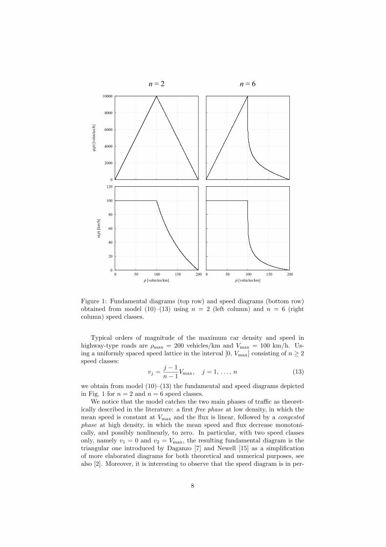
Figure 1: Fundamental diagrams (top row) and speed diagrams (bottom row)obtained from model (10)–(13) using n = 2 (left column) and n = 6 (rightcolumn) speed classes.

Typical orders of magnitude of the maximum car density and speed inhighway-type roads are ρmax = 200 vehicles/km and Vmax = 100 km/h. Us-ing a uniformly spaced speed lattice in the interval [0, Vmax] consisting of n ≥ 2speed classes:

vj =j − 1

n− 1Vmax, j = 1, . . . , n (13)

we obtain from model (10)–(13) the fundamental and speed diagrams depictedin Fig. 1 for n = 2 and n = 6 speed classes.

We notice that the model catches the two main phases of traffic as theoret-ically described in the literature: a first free phase at low density, in which themean speed is constant at Vmax and the flux is linear, followed by a congestedphase at high density, in which the mean speed and flux decrease monotoni-cally, and possibly nonlinearly, to zero. In particular, with two speed classesonly, namely v1 = 0 and v2 = Vmax, the resulting fundamental diagram is thetriangular one introduced by Daganzo [7] and Newell [15] as a simplificationof more elaborated diagrams for both theoretical and numerical purposes, seealso [2]. Moreover, it is interesting to observe that the speed diagram is in per-

8

fect agreement with that obtained numerically in [8] by simulating a microscopic“follow-the-leader” model. This confirms practically that the kinetic approachsuccessfully retains the microscopic character of car-to-car interactions, althoughthe representation of the system is not focused on single vehicles. Increasing thenumber of speed classes produces a stronger nonlinear trend of both fundamen-tal relationships in the congested phase, yet the critical density σ at which thephase transition occurs is always σ = ρmax

2 = 100 vehicles/km (we will provethis property, among other ones, in the next Section 3). This is ultimately dueto the fact that our prototypical table of games (12a)-(12b) lacks a parame-ter related to the environment (such as e.g., the quality of the road, weatherconditions), which can account for different driver behaviors in different roads.For more precise models detailing also this aspect we refer interested readersto [1, 10]. However, it is worth stressing that even such a simple model is able topredict the macroscopic phase transition as a consequence of more elementarylower scale car-to-car dynamics. Particularly, it does not require an ad hoc con-struction in which such a transition is given as an external input to the modelitself. To date, this seems to be impossible in a purely macroscopic approach,where the phase transition has to be postulated heuristically, cf. e.g., [3, 5].

3 Asymptotic analysis and equilibria

In this section we study the qualitative properties of system (10), particularly itsasymptotic trends and equilibria which, as stated in Section 2, are at the basisof the characterization of fundamental relationships. For the sake of simplicity,we consider the dimensionless version of the model in which the fj ’s and ρ arescaled with respect to ρmax, so that the maximum dimensionless density is 1,and likewise the vj ’s are scaled with respect to Vmax, so that the maximumdimensionless speed is vn = 1. In practice, we use Eqs. (10)–(13) with ρmax =Vmax = 1.

To begin with, we notice that, owing to the assumption that the interactionrate is independent of the speeds of the interacting vehicles, cf. Eq. (11), thespatially homogeneous equations (10) can be rewritten as:

dfjdt

= η[ρ]

n∑h, k=1

Ajhk[ρ]fhfk − ρfj

, j = 1, . . . , n, (14)

where we have further stressed that both η and the Ajhk’s depend on ρ. Byprescribing an initial condition f0 = (f01 , . . . , f

0n) ∈ Rn we obtain a Cauchy

problem, which well-posedness has been established in [9]. We report here thestatement of the result for completeness.

Theorem 3.1. Let f0 be such that

f0j ≥ 0 ∀ j = 1, . . . , n,

n∑j=1

f0j = ρ ∈ [0, 1].

There exists a unique global solution f = (f1, . . . , fn) ∈ C1((0, +∞); Rn) toEq. (14) such that f(0) = f0 and:

fj(t) ≥ 0 ∀ j = 1, . . . , n,

n∑j=1

fj(t) = ρ

9

for all t > 0.Moreover, given two initial data f0, g0 with the same density ρ the following

a priori continuity estimate holds true:

‖g(t)− f(t)‖1 + ‖g′(t)− f ′(t)‖1 ≤ (1 + 3η0)e3η0t‖g0 − f0‖1, ∀ t > 0,

where η0 := supρ∈[0, 1] η[ρ] and ‖ · ‖1 is the 1-norm in Rn. In particular, theabove estimate is uniform in time in every interval [0, T ], T < +∞.

Since the solution to Eq. (14) is global in time, it makes sense to investigateits asymptotic behavior for t → +∞. A first result is proved again in [9] andconcerns the existence of equilibria:

Theorem 3.2. For every ρ ∈ [0, 1] there exists at least one equilibrium pointf∞ = (f∞1 , . . . , f∞n ) ∈ Rn of Eq. (14) such that:

f∞j ≥ 0 ∀ j = 1, . . . , n,

n∑j=1

f∞j = ρ. (15)

Theorems 3.1 and 3.2 are quite general, in that they do not assume anyspecific expression of η[ρ] and Ajhk[ρ]. As a matter of fact, the only reallyimportant properties (besides non-negativity, obvious for modeling purposes)are that η[ρ] be bounded and the Ajhk[ρ]’s satisfy Eq. (7) for every ρ ∈ [0, 1].

A detailed expression of the table of games is instead necessary in order tocharacterize the uniqueness and stability of equilibria. Some studies on thisissue have been performed in [9], however they have been limited to a restrictednumber of speed classes, specifically n = 2, 3, while a result for generic n ≥ 2is still missing. The next theorem, proposed here for the first time, contributesto filling such a gap by taking advantage of the table (12a)-(12b).

Theorem 3.3. Let the transition probabilities be as in Eqs. (12a), (12b). Forevery n ≥ 2 and every ρ ∈ [0, 1] there exists a unique equilibrium point f∞ ofEq. (14) satisfying (15) and which is also stable and attractive.

Proof. Let f∞ be any of the equilibria that Theorem 3.2 speaks of. If ρ = 0then the unique possibility is trivially f∞j = 0 for all j = 1, . . . , n; therefore wewill henceforth focus on the case 0 < ρ ≤ 1.

First, we observe that it is sufficient to prove the uniqueness of the firstn − 1 components of f∞, for then the n-th one is uniquely determined by theconservation of mass:

f∞n = ρ−n−1∑j=1

f∞j .

Equilibria of system (14) solve the equation:

n∑h, k=1

Ajhk[ρ]f∞h f∞k − ρf∞j = 0, (16)

that, owing to the argument above, we only need to consider for j = 1, . . . , n−1.In order to follow the two cases h ≤ k and h > k which define the table of games

10

(cf. Eqs. (12a) and (12b), respectively), we split Eq. (16) as:

n∑h=1

n∑k=h

Ajhk[ρ]f∞h f∞k︸ ︷︷ ︸h≤k

+

n∑h=2

h−1∑k=1

Ajhk[ρ]f∞h f∞k︸ ︷︷ ︸h>k

−ρf∞j = 0 (17)

and then we prove the uniqueness of a stable and attractive f∞ by proceedingby induction on j.

Basis: f∞1 is unique.

If j = 1 the only nonzero coefficients of the table of games are:

i) for h ≤ k, A11k[ρ] = ρ (k = 1, . . . , n);

ii) for h > k, A1h1[ρ] = ρ (h = 2, . . . , n).

Hence Eq. (17) specializes as:

ρ

(n∑k=1

f∞k +n∑h=2

f∞h − 1

)f∞1 = 0,

which, using∑nk=1 f

∞k = ρ and consequently

∑nh=2 f

∞h = ρ− f∞1 , gives

ρ(2ρ− 1− f∞1 )f∞1 = 0.

The two solutions are (f∞1 )I = 0 and (f∞1 )II = 2ρ − 1. In order to studytheir stability, we notice that the calculations just made also imply that theright-hand side of Eq. (14) for j = 1 is η[ρ](−ρf21 + ρ(2ρ − 1)f1), namely asecond degree polynomial in f1 with negative leading coefficient, whose rootsare precisely the two possible values of f∞1 found above. It is a basic fact ofstability theory that, in such a case, the only stable equilibrium, which is alsoattractive, coincides with the larger root, whereas the other one is unstable.Hence the first component of f∞ is univocally determined by choosing:

f∞1 =

{0 if ρ ≤ 1

2

2ρ− 1 if ρ > 12 .

(18)

Inductive step: if f∞1 , . . . , f∞j−1 are unique then so is f∞j .

For 2 ≤ j ≤ n− 1 the only nonzero coefficients of the table of games are:

i) for h ≤ k, Ajjk[ρ] = ρ (k = j, . . . , n) and Ajj−1,k[ρ] = 1 − ρ (k = j −1, . . . , n);

ii) for h > k, Ajhj [ρ] = ρ (h = j+1, . . . , n) and Ajjk[ρ] = 1−ρ (k = 1, . . . , j−1),

thus Eq. (17) specializes as:

ρf∞j

n∑k=j

fk + (1− ρ)f∞j−1

n∑k=j−1

f∞k︸ ︷︷ ︸h≤k

+ ρf∞j

n∑h=j+1

f∞h + (1− ρ)f∞j

j−1∑k=1

f∞k︸ ︷︷ ︸h>k

− ρf∞j = 0.

11

Using the conservation of mass as before for replacing conveniently the sums upto n with sums up to at most j and rearranging the terms we finally discover:

−ρ(f∞j )2

+

[(1− 3ρ)

j−1∑k=1

f∞k + ρ(2ρ− 1)

]f∞j +(1−ρ)f∞j−1

(ρ−

j−2∑k=1

f∞k

)= 0,

(19)which, since by the inductive hypothesis f∞1 , . . . , f∞j−1 are known, is a seconddegree polynomial equation in the unknown f∞j . The discriminant

∆ =

[(1− 3ρ)

j−1∑k=1

f∞k + ρ(2ρ− 1)

]2+ 4ρ(1− ρ)f∞j−1

(ρ−

j−2∑k=1

f∞k

)(20)

being positive for all 0 < ρ ≤ 1, there are two real roots whose only the largerone is a stable and attractive equilibrium, because the leading coefficient ofthe polynomial is negative. In addition, by inspecting the constant term afterrewriting the polynomial in monic form (i.e., collecting −ρ at the left-hand side)we infer that the product of the two roots is negative, hence the larger one isnecessarily positive. Finally, we conclude that the admissible (viz. stable andnonnegative) f∞j is unique.

From the proof of Theorem 3.3 we can deduce the following recursive formulafor the components of the equilibrium f∞:

f∞j =

{0 if ρ ≤ 1

2

2ρ− 1 if ρ > 12

if j = 1

−

[(1− 3ρ)

j−1∑k=1

f∞k + ρ(2ρ− 1)

]+√

∆

2ρif 2 ≤ j ≤ n− 1

ρ−n−1∑k=1

f∞k if j = n,

where ∆ is given by Eq. (20). Notice that for 2 ≤ j ≤ n − 1 we have chosenthe solution to Eq. (19) with the positive sign in front of the square root of ∆because it is certainly the larger one.

If ρ ≤ 12 then it results f∞j = 0 for all j = 1, . . . , n− 1 and f∞n = ρ, which

implies that the flux and mean speed at equilibrium are, respectively,

q(ρ) = vnf∞n = ρ, u(ρ) =

1

ρvnf

∞n = 1

regardless of the number n of speed classes. This explains the same trendobserved in Fig. 1 in the free phase for both n = 2 and n = 6. Notice that u isactually indeterminate for ρ = 0 but can be extended by continuity.

Conversely, if ρ > 12 the trend of q and u depends on n, as it is also evident

from Fig. 1 itself. In the case n = 2 it is not difficult to compute explicitly thesetrends for all ρ. We have indeed:

f∞1 =

{0 if ρ ≤ 1

2

2ρ− 1 if ρ > 12 ,

f∞2 =

{ρ if ρ ≤ 1

2

1− ρ if ρ > 12

12

and v1 = 0, v2 = 1, whence

q(ρ) = f∞2 =

{ρ if ρ ≤ 1

2

1− ρ if ρ > 12 ,

u(ρ) =1

ρf∞2 =

{1 if ρ ≤ 1

21ρ − 1 if ρ > 1

2 ,

which confirms the triangular-shaped flux with critical density σ = 12 at road

capacity (phase transition).As anticipated in Section 2.1, the proof of Theorem 3.3 indicates that the

critical density for model (10)–(13) is invariably σ = 12 , namely σ = ρmax

2 indimensional form, independently of the number of speed classes. In more detail,when ρ crosses such a σ a supercritical bifurcation occurs: for ρ < σ thereactually exists only the stable equilibrium (f∞1 )I = 0, because (f∞1 )II = 2ρ− 1is negative and thus non admissible; for ρ > σ the equilibrium (f∞1 )I still existsbut becomes unstable, while the new stable equilibrium (f∞1 )II appears.

References

[1] A. Bellouquid, E. De Angelis, and L. Fermo. Towards the modeling ofvehicular traffic as a complex system: a kinetic theory approach. Math.Models Methods Appl. Sci., 22(supp01):1140003 (35 pages), 2012.

[2] S. Blandin, G. Bretti, C. Cutolo, and B. Piccoli. Numerical simulations oftraffic data via fluid dynamic approach. Appl. Math. Comput., 210(2):441–454, 2009.

[3] S. Blandin, D. Work, P. Goatin, B. Piccoli, and A. Bayen. A general phasetransition model for vehicular traffic. SIAM J. Appl. Math., 71(1):107–127,2011.

[4] I. Bonzani and L. Mussone. From experiments to hydrodynamic trafficflow models. I. Modelling and parameter identification. Math. Comput.Modelling, 37(12-13):1435–1442, 2003.

[5] R. M. Colombo. Hyperbolic phase transitions in traffic flow. SIAM J. Appl.Math., 63(2):708–721, 2002.

[6] V. Coscia, M. Delitala, and P. Frasca. On the mathematical theory ofvehicular traffic flow. II. Discrete velocity kinetic models. Internat. J. Non-Linear Mech., 42(3):411–421, 2007.

[7] C. F. Daganzo. A variational formulation of kinematic waves: Solutionmethods. Transport. Res. B-Meth., 39(10):934–950, 2005.

[8] P. Degond and M. Delitala. Modelling and simulation of vehicular trafficjam formation. Kinet. Relat. Models, 1(2):279–293, 2008.

[9] M. Delitala and A. Tosin. Mathematical modeling of vehicular traffic: a dis-crete kinetic theory approach. Math. Models Methods Appl. Sci., 17(6):901–932, 2007.

[10] L. Fermo and A. Tosin. A fully-discrete-state kinetic theory approach tomodeling vehicular traffic. SIAM J. Appl. Math., 2013. In press.

13

[11] M. Garavello and B. Piccoli. Traffic flow on networks – Conservation lawsmodels, volume 1 of AIMS Series on Applied Mathematics. American In-stitute of Mathematical Sciences (AIMS), Springfield, MO, 2006.

[12] M. Gunther, A. Klar, T. Materne, and R. Wegener. Multivalued fundamen-tal diagrams and stop and go waves for continuum traffic flow equations.SIAM J. Appl. Math., 64(2):468–483, 2003.

[13] B. S. Kerner. The Physics of Traffic. Springer, Berlin, 2004.

[14] J. Li and M. Zhang. Fundamental diagram of traffic flow. Transp. Res.Record, 2260:50–59, 2011.

[15] G. F. Newell. A simplified theory of kinematic waves in highway traffic, partII: Queueing at freeway bottlenecks. Transport. Res. B-Meth., 27(4):289–303, 1993.

[16] B. Piccoli and A. Tosin. Vehicular traffic: A review of continuum mathe-matical models. In R. A. Meyers, editor, Encyclopedia of Complexity andSystems Science, volume 22, pages 9727–9749. Springer, New York, 2009.

14