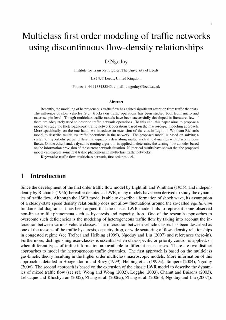
1

Multiclass first order modeling of traffic networksusing discontinuous flow-density relationships

D.NgoduyInstitute for Transport Studies, The University of Leeds

LS2 9JT Leeds, United Kingdom

Phone: + 44 1133435345, e-mail: d.ngoduy@leeds.ac.uk

Abstract

Recently, the modeling of heterogeneous traffic flow has gained significant attention from traffic theorists.The influence of slow vehicles (e.g. trucks) on traffic operations has been studied both from micro andmacroscopic level. Though multiclass traffic models have been successfully developed in literature, few ofthem are adequately used to describe traffic network operations. To this end, this paper aims to propose amodel to study the (heterogeneous) traffic network operations based on the macroscopic modeling approach.More specifically, on the one hand, we introduce an extension of the classic Lighthill-Whitham-Richardsmodel to describe multiclass traffic operations in the network. The proposed model is based on solving asystem of hyperbolic partial differential equations describing multiclass traffic dynamics with discontinuousfluxes. On the other hand, a dynamic routing algorithm is applied to determine the turning flow at nodes basedon the information provision of the current network situation. Numerical results have shown that the proposedmodel can capture some real traffic phenomena in multiclass traffic networks.

Keywords: traffic flow, multiclass network, first order model.

1 Introduction

Since the development of the first order traffic flow model by Lighthill and Whitham (1955), and indepen-dently by Richards (1956)-hereafter denoted as LWR, many models have been derived to study the dynam-ics of traffic flow. Although the LWR model is able to describe a formation of shock wave, its assumptionof a steady-state speed density relationship does not allow fluctuations around the so-called equilibriumfundamental diagram. It has been argued that the classic LWR model fails to represent some observednon-linear traffic phenomena such as hysteresis and capacity drop. One of the research approaches toovercome such deficiencies is the modeling of heterogeneous traffic flow by taking into account the in-teraction between various vehicle classes. The interaction between vehicle classes has been described asone of the reasons of the traffic hysteresis, capacity drop, or wide scattering of flow- density relationshipsin congested regime (see Treiber and Helbing (1999), Ngoduy and Liu (2007) and references there-in).Furthermore, distinguishing user-classes is essential when class-specific or priority control is applied, orwhen different types of traffic information are available to different user-classes. There are two distinctapproaches to model the heterogeneous traffic dynamics. The first approach is based on the multiclassgas-kinetic theory resulting in the higher order multiclass macroscopic models. More information of thisapproach is detailed in Hoogendoorn and Bovy (1999), Helbing et al. (1999a), Tampere (2004), Ngoduy(2006). The second approach is based on the extension of the classic LWR model to describe the dynam-ics of mixed traffic flow (see ref. Wong and Wong (2002), Logghe (2003), Chanut and Buisons (2003),Lebacque and Khoshyaran (2005), Zhang et al. (2006a), Zhang et al. (2006b), Ngoduy and Liu (2007)).

2 D.NGODUY

Theoretically, the higher order models have been able to show some significant improvements over the firstorder models in replicating the transitions between congested traffic states: stop-and-go waves, movingclusters, oscillatory congested traffic, etc. (see Kerner (2004), Helbing and Treiber (1998), Helbing et al.(1999b), Ngoduy (2008)). However, the former also generate higher number of parameters and requiremore complicated numerical solution than the latter. Therefore, different modeling approaches will beadopted according to various applications.

In general, most of the multiclass models developed so far mainly focus on the description of trafficdynamics on freeways. In principle, a traffic network consists of a set of nodes (intersections) and a setof links. Traffic originates at origin nodes and is directed to destination nodes via chosen paths that aredetermined from a traffic assignment model or route-choice model. The route-choice model is then usedto determine the fraction of traffic going from one link to the others, which is used as an input to predicttraffic dynamics of links. The difficulty stems from the modeling of the dynamics of traffic flow at nodesgiven certain traffic demands. In literature, the macroscopic description of traffic flow dynamics in roadnetworks using higher order models has been proposed in Garavello and Piccoli (2006), Herty and Rascle(2006). However, extension of such higher order macroscopic models to multi-class networks generallyrequires very complex numerical implementation at nodes. A few first order macroscopic models fortraffic networks have been proposed in Elloumi et al. (1994) and Buisson et al. (1996) but these modelsrarely distinguish user classes. Although the models of Lebacque and Khoshyaran (2005) and Herty et al.(2006) deal with multiclass traffic networks, their underlying assumption of homogeneous desired speedsfor all vehicle classes does not permit overtaking driving behavior, which is an important characteristicof multiclass traffic operations. To this end, we propose in this paper a generalized first order modelfor multiclass traffic operations in the network. The model is based on solving a system of hyperbolicpartial differential equations describing the first order multi-class traffic model with discontinuous fluxes.Discussion of the problems of the system of hyperbolic partial differential equations with discontinuousfluxes has been formulated in detail in Zhang et al. (2006b) and references there-in. In our model, thedynamic routing algorithm is applied to determine the turning flow at nodes based on the informationprovision of the current network situation. This paper is organized as follows. Section 2 illustrates thegoverning equations for the multiclass first order traffic model on links. In Section 3, we propose amulticlass (first order) simulation model for traffic dynamics at nodes in the network. Section 4 formulatesa simple dynamic routing algorithm given the information about the current network situation. Section 5illustrates some numerical results, followed by discussions. Finally, we conclude the paper in Section 6.

2 Governing equations for multiclass first order model

As a basis, a traffic network is represented as a directed graph (Figure 1), in which nodes (origins, destina-tions and intermediate nodes) are connected through directed links. In our paper, the traffic dynamics onlinks are described by the multiclass LWR model presented in the framework of Wong and Wong (2002),Zhang et al. (2006a), Ngoduy and Liu (2007). Let us first recall the concept of the multiclass LWR model.Let u(u ∈ U) denote the vehicle class index. Let ru

a(x, t), V ua (x, t) and qu

a(x, t) denote the class specificdensity, mean speed and flow of link a (a = 1,2, ...,A), respectively. From the conservation law, eachvehicle class should satisfy the following equation:

∂rua

∂t+

∂qua

∂x= 0 ∀u ∈ U (1)

D.NGODUY 3

Fig. 1. Network description: a directed graph.

Equation (1) can be written in the vector form:

∂ra

∂t+

∂qa

∂x= 0 (2)

where

ra =

r1a

r2a

...rUa

, qa =

q1a

q2a

...qUa

(3)

The properties of the proposed multiclass model are discussed analytically and numerically by Ngoduyand Liu (2007). Set of equations (1) is complete if the speed-density or flow-density relationship (so-called fundamental diagram) is known for every link: qu

a = qua

(r1a, r

2a, ..., r

Ua

). There are many choices of

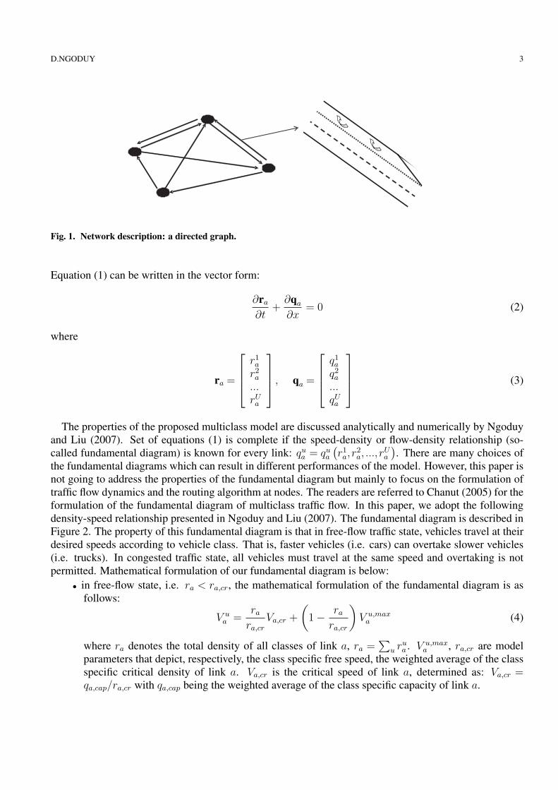
the fundamental diagrams which can result in different performances of the model. However, this paper isnot going to address the properties of the fundamental diagram but mainly to focus on the formulation oftraffic flow dynamics and the routing algorithm at nodes. The readers are referred to Chanut (2005) for theformulation of the fundamental diagram of multiclass traffic flow. In this paper, we adopt the followingdensity-speed relationship presented in Ngoduy and Liu (2007). The fundamental diagram is described inFigure 2. The property of this fundamental diagram is that in free-flow traffic state, vehicles travel at theirdesired speeds according to vehicle class. That is, faster vehicles (i.e. cars) can overtake slower vehicles(i.e. trucks). In congested traffic state, all vehicles must travel at the same speed and overtaking is notpermitted. Mathematical formulation of our fundamental diagram is below:

• in free-flow state, i.e. ra < ra,cr, the mathematical formulation of the fundamental diagram is asfollows:

V ua =

ra

ra,cr

Va,cr +

(1− ra

ra,cr

)V u,max

a (4)

where ra denotes the total density of all classes of link a, ra =∑

u rua . V u,max

a , ra,cr are modelparameters that depict, respectively, the class specific free speed, the weighted average of the classspecific critical density of link a. Va,cr is the critical speed of link a, determined as: Va,cr =qa,cap/ra,cr with qa,cap being the weighted average of the class specific capacity of link a.

4 D.NGODUY

0 20 40 60 80 1000

10

20

30

40

50

60

70

80

90

100

110

Density (veh/km)

Spe

ed (

km/h

)

Speed−Density Relationship

Fast car (class 1)Slow car (class 2)Truck (class 3)

rcr r

jam

V1,max

V2,max

V3,max

Fig. 2. Fundamental diagram for multiclass traffic flow.

• in congested state i.e. ra ≥ ra,cr:

V ua =

ra,jam − ra

(ra,jam − ra,cr) ra

Va,crra,cr =ra,jam − ra

(ra,jam − ra,cr) ra

qa,cap (5)

where ra,jam denotes the weighted average of the class specific jam density of link a.Note that all the weighted values of model parameters are determined by the following equation:

ra,cr = r0a,cr

U∑u=1

αua

γu, qa,cap = q0

a,cap

U∑u=1

αua

γu, ra,jam = r0

a,jam

U∑u=1

αua

γu(6)

where r0a,cr, r0

a,jam and q0a,cap denote, respectively, the critical density, jam density and capacity of a refer-

ence class, which are determined in passenger car units (pcu). γu denotes the pcu factor of vehicle class u,which represents the differences in the amount of interference to other traffic in mixed traffic operations.For example, a truck has a considerably greater effect on other vehicles by making it more difficult forthem to overtake and by slowing down those which are forced to follow. Typical values of the pcu factorare given in Highway Capacity Manual (2000). αu is the share factor of vehicle class u. By definition, wehave αu

a = rua/

∑u ru

a = rua/ra.

It is worthy to mention that in the congested regime the class specific speed is homogeneous (i.e.V 1

a (∑

u ru) = V 2a (

∑u ru) = ... = V U

a (∑

u ru)), resulting in a contact discontinuity with homogeneouseigenvalues, which are equal to the traffic speed. In Zhang et al. (2006a) the authors have thoroughly ana-lyzed many important mathematical issues regarding the mechanism for the formation of shock, expansionwaves and contact discontinuity in a class of system of hyperbolic partial differential equations. Readersare referred to Zhang et al. (2006a) for more detailed discussion.

Let λu denote the eigenvalues of equation (2), which represents the propagation of the characteristicsof different vehicle classes (here the index a has been dropped for simplicity). System of equations (2) isstrictly hyperbolic if λu are all real and distinct. That is:

λu ∈ R ∀u ∈ U, λ1a < λ2 <, ..., < λU (7)

D.NGODUY 5

For U = 2, it is straightforward to obtain:

λ1 = 0.5

[c11 + c22−

√(c11− c22)2 + 4c12c21

]

λ2 = 0.5

[c11 + c22 +

√(c11− c22)2 + 4c12c21

](8)

wherecuu = V u + ru dV u

dru, cus = ru dV u

drs∀u 6= s (9)

By substituting (9) to (8), it can be proved that (7) is satisfied with U = 2. General analytical proof ofthe hyperbolic property of system (2) can be found in Zhang et al. (2006a) for U > 2. Accordingly, thestandard well-posed theory of the hyperbolic system and the corresponding numerical solutions apply. Tothis end, several numerical schemes have been developed to to solve the model. For example, the modelsof Wong and Wong (2002) and Zhang et al. (2006a) are based on the finite difference scheme family:Lax-Friedrichs and higher order weighted essentially non-oscillatory (WENO) scheme, respectively. Notethat the latter is actually based on the Lax-Friedrichs flux splitting scheme for the fifth order accuracy. Analternative approach is based on the (first order) finite volume method, for example in Ngoduy and Liu(2007). The rest of this section summarizes the simulation model of multiclass traffic flow presented inNgoduy and Liu (2007). Let time and space be divided separately into time steps tk = k∆t (k = 1...K) andsegments (or cells) xi = i∆x (i = 1...I). Note that the time step and cell length are chosen to satisfy theCourant-Friedrichs-Lewy (CFL) condition Sod (1985): ∆x ≥ V U,max∆t, where V U,max denotes the freespeed of the fastest vehicle. Note that in this paper we set ∆x equally for every link. The space-averagedconservation vector ra in system (2) over cell i at time instant k is defined as ra(i,k). The approximationsolution at the next time step is then obtained by:

ra(i, k + 1) = ra(i, k)− ∆t

∆x(qa(i + 1/2, k)− qa(i− 1/2, k)) (10)

where qa(i + 1/2,k) denotes the numerical flux at cell interface xi+1/2 of link a, which is computed as:

qa(i + 1/2,k) =χ+

i+1/2qa(i,k)−χ−i+1/2qa(i + 1,k)

χ+i+1/2−χ−i+1/2

+χ+

i+1/2χ−i+1/2

χ+i+1/2−χ−i+1/2

(ra(i + 1,k)− ra(i,k)) (11)

where qa(i, k) =[q1a(i,k), q2

a(i,k), ..., qUa (i,k)

]. The class specific flow qu

a(i, k) is determined from thefundamental diagram of link a based on the class specific density ru

a(i, k) at cell i and time instant k.χ+

i+1/2 and χ−i+1/2 are the upper bounds and lower bounds of the largest and smallest physical wave speedsat cell interface xi+1/2. These quantities are applied in order to capture the differences between free-flow and congested flow conditions. For example, the disturbances in the free-flow traffic moving in thedownstream direction (along the two characteristics defined by dx± = χ±dt) can be determined as:

χ+i+1/2 = max

(χR

i+1/2, 0), χ−i+1/2 = min

(χL

i+1/2, 0)

(12)

The variables χRi+1/2 and χL

i+1/2 in equation (12) denote the numerical approximations for the largest andsmallest physical wave speeds, respectively, of the shock wave propagation in the exact solution of theRiemann problem determined as follows:

χRi+1/2 = max

(λmax

i+1/2, λmaxi+1

), χL

i+1/2 = min(λmin

i+1/2, λmini

)(13)

6 D.NGODUY

where λmaxi = max (λu

i , u = 1,2, ...,U) and λmini = min (λu

i , u = 1,2, ...,U). Similarly, λmaxi+1/2 =

max(λu

i+1/2, u = 1,2, ...,U)

and λmini+1/2 = min

(λu

i+1/2, u = 1,2, ...,U)

. Here λui and λu

i+1/2 denotethe eigenvalues of system (2) calculated at the cell i and cell interface i+1/2, respectively. It is worthy tonotice from expression (13) that χ+

i+1/2−χ−i+1/2 is not able to approach 0. In free-flow state, the charac-teristic is moving downstream so χ+

i+1/2 > 0 and χ−i+1/2 = 0, whereas in congested state, the characteristicis moving upstream so χ+

i+1/2 = 0 and χ−i+1/2 < 0.Set of equations (10) - (13) complete the simulation model for multiclass traffic dynamics on links given

the class specific inflow and outflow at the upstream and downstream nodes (boundary conditions). Theclass specific inflow and outflow at nodes are calculated through a node model, which is the aim of thenext section.

3 Traffic flow dynamics at nodesThe macroscopic models of traffic flow dynamics at nodes has been intensively studied in mathematicalaspects by Holden and Risebro (1995), Coclite and Piccoli (2005) in which the mathematical issues suchas the weak solution concept, the entropy condition and the well-posedness of the problem at the node arewell dealt with. The development of (first order) multi-class traffic models for traffic networks has beenproposed recently by Lebacque and Khoshyaran (2005), Herty et al. (2006). The underlying assumptionof those multiclass models is that all vehicles have the same desired speed. Therefore, all vehicles willoperate with the same speed. i.e. V 1

a = V 2a = ... = V U

a = Va. Accordingly, equation (1) is reduced to:

∂ra

∂t+

∂qa

∂x= 0, (14)

∂αua

∂t+ Va

∂αua

∂x= 0. (15)

Equation (15) means that the share factor is unchanged along the vehicle trajectories. As a result, noovertaking is allowed in those models. In this paper, we have relaxed this assumption by solving equation(1) as a system of hyperbolic partial differential equations with distinct eigenvalues, which model theovertaking behavior in the context of multi-class traffic operations.

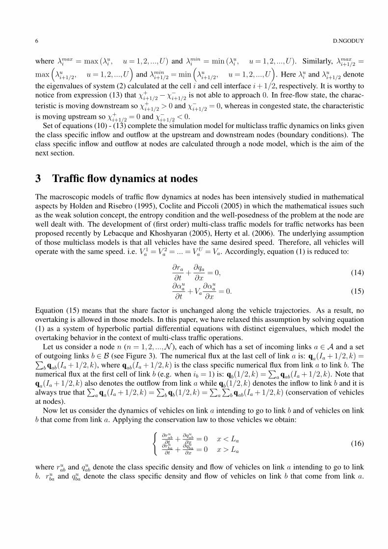
Let us consider a node n (n = 1,2, ...,N ), each of which has a set of incoming links a ∈ A and a setof outgoing links b ∈ B (see Figure 3). The numerical flux at the last cell of link a is: qa(Ia + 1/2, k) =∑

b qab(Ia + 1/2, k), where qab(Ia + 1/2,k) is the class specific numerical flux from link a to link b. Thenumerical flux at the first cell of link b (e.g. when ib = 1) is: qb(1/2,k) =

∑a qab(Ia + 1/2,k). Note that

qa(Ia + 1/2,k) also denotes the outflow from link a while qb(1/2,k) denotes the inflow to link b and it isalways true that

∑a qa(Ia + 1/2,k) =

∑b qb(1/2,k) =

∑a

∑b qab(Ia + 1/2,k) (conservation of vehicles

at nodes).Now let us consider the dynamics of vehicles on link a intending to go to link b and of vehicles on link

b that come from link a. Applying the conservation law to those vehicles we obtain:{

∂ruab

∂t+

∂quab

∂x= 0 x < La

∂ruba

∂t+

∂quba

∂x= 0 x > La

(16)

where ruab and qu

ab denote the class specific density and flow of vehicles on link a intending to go to linkb. ru

ba and quba denote the class specific density and flow of vehicles on link b that come from link a.

D.NGODUY 7

n

Inlinks a Outlinks b

Fig. 3. The configuration of a node.

Let βuab denote the (dynamic) class specific fraction of vehicles from link a to link b (turning fraction).

By definition, quab = βu

abqua . The class specific turning fraction is determined from a routing algorithm

presented in the next section of this paper. Moreover, we define quba = φu

baqub , where φu

ba is the class specificspace coefficient that accounts for the partial space of link b used for traffic from link a. There are a fewmethods to calculate φu

ba (see Lebacque and Khoshyaran (2005)). In this paper, we adopt the followingformula for φu

ba:

φuba =

quab∑A

a=1 quab

=βu

abqua∑A

a=1 βuabq

ua

(17)

Equation (17) reflects the fact that the flows are shared according to the incoming flows from upstreamlinks. That means that the downstream link will allocate more space for the upstream link having higherinflows. It is worthy to mention that according to Lebacque and Khoshyaran (2005) equation (17) does notrespect the so-called invariance principle, which means that the class specific space coefficient is subjectto discontinuous changes in certain cases. However, Lebacque and Khoshyaran (2005) have claimed thatsuch violation of the invariance principle does not affect the discretized, phenomenological models, whichare the case in our proposed simulation model.

In general, qua and qu

b are determined from different fundamental diagrams that are specified for link aand link b, respectively. qu

ab and quba are also determined from different flow-density curves due to the turn-

ing fraction βuab and the space factor φu

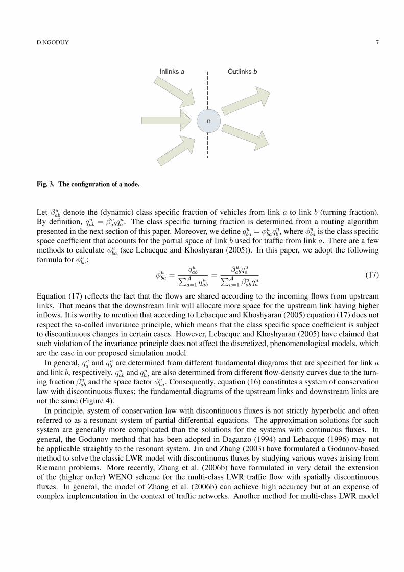
ba. Consequently, equation (16) constitutes a system of conservationlaw with discontinuous fluxes: the fundamental diagrams of the upstream links and downstream links arenot the same (Figure 4).

In principle, system of conservation law with discontinuous fluxes is not strictly hyperbolic and oftenreferred to as a resonant system of partial differential equations. The approximation solutions for suchsystem are generally more complicated than the solutions for the systems with continuous fluxes. Ingeneral, the Godunov method that has been adopted in Daganzo (1994) and Lebacque (1996) may notbe applicable straightly to the resonant system. Jin and Zhang (2003) have formulated a Godunov-basedmethod to solve the classic LWR model with discontinuous fluxes by studying various waves arising fromRiemann problems. More recently, Zhang et al. (2006b) have formulated in very detail the extensionof the (higher order) WENO scheme for the multi-class LWR traffic flow with spatially discontinuousfluxes. In general, the model of Zhang et al. (2006b) can achieve high accuracy but at an expense ofcomplex implementation in the context of traffic networks. Another method for multi-class LWR model

8 D.NGODUY

0 50 100 1500

500

1000

1500

2000

2500

3000

3500

4000

4500

Density (veh/km)F

low

(ve

h/h)

Flow−density relationships

Upstream linkDownstream link

rcrb r

cra

qcapa

qcapb

Fig. 4. Discontinuous flow-density relationships

with discontinuous fluxes that is worthy to be mentioned is the hybrid scheme proposed by Zhang et al.(2008) in which the finite difference scheme WENO is reconstructed to resolve the waves more efficientlythan the standard WENO scheme in Zhang et al. (2006b).

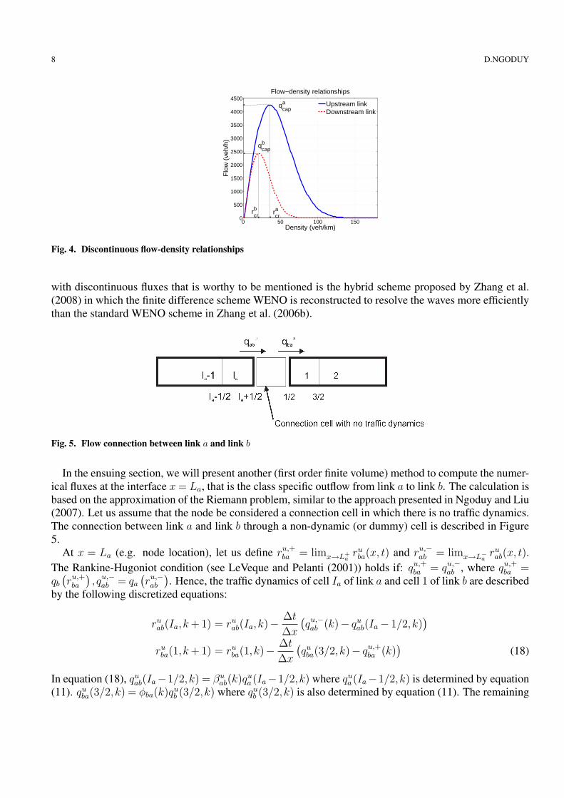
Fig. 5. Flow connection between link a and link b

In the ensuing section, we will present another (first order finite volume) method to compute the numer-ical fluxes at the interface x = La, that is the class specific outflow from link a to link b. The calculation isbased on the approximation of the Riemann problem, similar to the approach presented in Ngoduy and Liu(2007). Let us assume that the node be considered a connection cell in which there is no traffic dynamics.The connection between link a and link b through a non-dynamic (or dummy) cell is described in Figure5.

At x = La (e.g. node location), let us define ru,+ba = limx→L+

aruba(x, t) and ru,−

ab = limx→L−a ruab(x, t).

The Rankine-Hugoniot condition (see LeVeque and Pelanti (2001)) holds if: qu,+ba = qu,−

ab , where qu,+ba =

qb

(ru,+ba

), qu,−

ab = qa

(ru,−ab

). Hence, the traffic dynamics of cell Ia of link a and cell 1 of link b are described

by the following discretized equations:

ruab(Ia,k + 1) = ru

ab(Ia,k)− ∆t

∆x

(qu,−ab (k)− qu

ab(Ia− 1/2,k))

ruba(1,k + 1) = ru

ba(1,k)− ∆t

∆x

(quba(3/2,k)− qu,+

ba (k))

(18)

In equation (18), quab(Ia−1/2,k) = βu

ab(k)qua(Ia−1/2,k) where qu

a(Ia−1/2,k) is determined by equation(11). qu

ba(3/2,k) = φba(k)qub (3/2,k) where qu

b (3/2,k) is also determined by equation (11). The remaining

D.NGODUY 9

unknown functions are qu,−ab (k) and qu,+

ba (k). In general, the standard Godunov approximation for thenumerical flux of the conservation equations is computed in Godunov (1959) as:

F (a,b) = minr∈[a,b]

F (r) if a≤ b

F (a,b) = maxr∈[b,a]

F (r) if a≥ b (19)

where F denotes the concave function of the density r. Since F has one global maximum at r = rcr, wecan apply equation (19) to compute the numerical fluxes between cell Ia of link a and cell 1 of link b as:

qu,+ab (k) = qu,−

ba (k) = min

(quba

(rb,cr,

∑u

rub (1,k)

), qu

ab

(∑u

rua(Ia,k), ra,cr

))

= min

(φu

ba(k)qub

(rb,cr,

∑u

rub (1,k)

),βu

ab(k)qua

(∑u

rua(Ia,k), ra,cr

))(20)

where qua(.) and qu

b (.) are the function of density rua and ru

b , respectively. By comparing the weighted (link)critical density with the total density of the first cell/the last cell at each time step, we can determine qu

a(.)and qu

b (.) using equation (19).Note that in case u = 1 (e.g. homogeneous traffic flow), we have:

qb (rb,cr, rb(1,k)) = qb (rb(1,k)) if rb(1,k)≥ rb,cr

qb (rb,cr, rb(1,k)) = qb (rb,cr) = qb,cap if rb(1,k)≤ rb,cr

qa (ra(I,k), ra,cr) = qa (ra,cr) = qa,cap if ra(I,k)≥ ra,cr

qa (ra(I,k), ra,cr) = qa (ra(I,k)) if ra(I,k)≤ ra,cr. (21)

This calculation is similar to the supply and demand principle presented in Lebacque and Khoshyaran(2005). To complete the node model, the class specific turning fraction βu

ab needs to be determined. In ourpaper, βu

ab is considered a dynamic factor, determined from the instantaneous responses of drivers to theinformation of the current network situation. That is, drivers will switch to the other route if they find theinstantaneous travel time to their destination in the current route larger than in the new route. In the nextsection, we will present the routing algorithm that is incorporated into our network model.

4 Dynamics routing algorithmThis section presents a principle to compute the turning fraction at nodes in the multiclass traffic networks.Let pc denote the current possible path and po denote the best alternative path from junction n to destinationd at time instant k. The instantaneous travel time of vehicle class u, τu

p , from node n to destination d usingpath p (p = pc,po) is:

τup (k) =

∑c∈p

Lc

V̄ uc (k)

(22)

where c is the link index that belongs to path p. Lc is the length of link c. V̄ uc is the speed of vehicle class

u on link c, averaged over cells.At the next time step, all drivers are assumed to get information of the network situation and can evaluate

10 D.NGODUY

the travel time of the different routes. Consequently, they will switch from the current path to the bestalternative path if τu

pc− τu

po> 0. That is:

βuaa′(k + 1) =

{1− πu if τu

pc(k)− τu

po(k) > 0

πu if τupc

(k)− τupo

(k)≤ 0(23)

here a′ is the outgoing link index (from node n) that belongs to the current path pc. πu (πu ∈ [0,1])denotes the proportion of vehicle class u switching to the best past when receiving the information. Notein equation (23) that the route choice is made using the path travel time calculated from the previousiteration. This assumption is rather reasonable since the time step is small (e.g. a few seconds in manymacroscopic simulation models) and should not have large impact on the choice decision. The pseudocodes of our model are given below:

• Performing the shortest path algorithm to compute βuab(0)

• For k = 0,1,2, ...:1. Computing φu

ba(k) based on equation (17).2. Determining qu,+

ab (k) from equation (20).3. Computing the class specific density based on equations (10)-(13) and equation (18).4. Determining the corresponding class specific speed based on equations (4) and (5).5. Computing the travel time from equation (22).6. Updating βu

ab(k + 1) based on equation (23) and then repeating all calculations from Step 1.With the optimal route from each node to all destinations, we can create a routing table for each node.

The table is updated at each time step during the simulation. Nevertheless, equation (23) may reflect an ex-tremely simplified behavior. The switching behavior can be operationalized with a decision rule, wherebythe driver switches from his current path only if the improvement in remaining travel time exceeds somethreshold level (Mahmassani and Jayakrishnan, 1991). In the model of Mahmassani and Jayakrishnan(1991) the threshold level may reflect perceptual factors, preferential indifference, or persistence and aver-sion to switching. However, for the illustration purposes, we adopt our simple routing principle (23) withπu = 1 for the time beings to study the multiclass traffic flow dynamics at nodes.

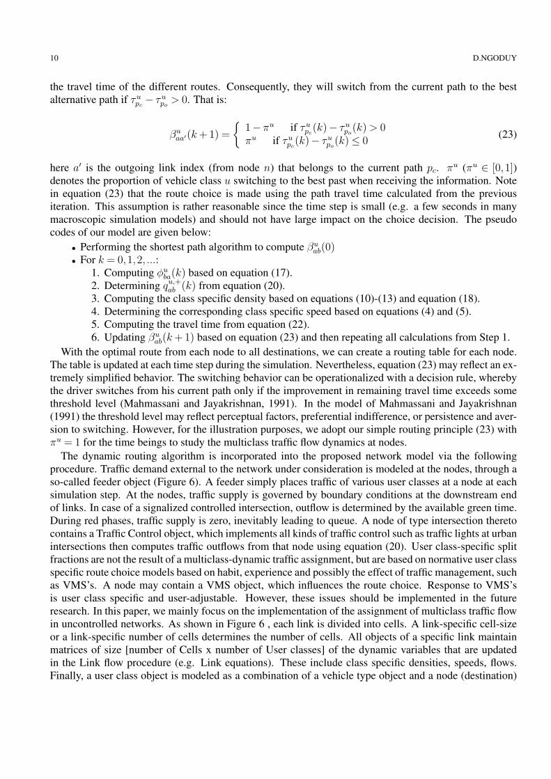
The dynamic routing algorithm is incorporated into the proposed network model via the followingprocedure. Traffic demand external to the network under consideration is modeled at the nodes, through aso-called feeder object (Figure 6). A feeder simply places traffic of various user classes at a node at eachsimulation step. At the nodes, traffic supply is governed by boundary conditions at the downstream endof links. In case of a signalized controlled intersection, outflow is determined by the available green time.During red phases, traffic supply is zero, inevitably leading to queue. A node of type intersection theretocontains a Traffic Control object, which implements all kinds of traffic control such as traffic lights at urbanintersections then computes traffic outflows from that node using equation (20). User class-specific splitfractions are not the result of a multiclass-dynamic traffic assignment, but are based on normative user classspecific route choice models based on habit, experience and possibly the effect of traffic management, suchas VMS’s. A node may contain a VMS object, which influences the route choice. Response to VMS’sis user class specific and user-adjustable. However, these issues should be implemented in the futureresearch. In this paper, we mainly focus on the implementation of the assignment of multiclass traffic flowin uncontrolled networks. As shown in Figure 6 , each link is divided into cells. A link-specific cell-sizeor a link-specific number of cells determines the number of cells. All objects of a specific link maintainmatrices of size [number of Cells x number of User classes] of the dynamic variables that are updatedin the Link flow procedure (e.g. Link equations). These include class specific densities, speeds, flows.Finally, a user class object is modeled as a combination of a vehicle type object and a node (destination)

D.NGODUY 11

Fig. 6. Model of dynamic route choice and link flow

object. A vehicle type object incorporates all parameters associated with different types of driver-vehiclecombinations: free speed, capacity, jam density and critical density.

5 Numerical studiesThis section is devoted to the numerical studies of our network model. On the one hand, the approximationsolution for multiclass traffic flow dynamics with discontinuous fundamental diagrams is investigated. Onthe other hand, the full network model is simulated.

5.1 Traffic dynamics with discontinuous fundamental diagramsThe purpose of this section is to describe the performance of the proposed approximation solution incalculating the propagation of multiclass traffic flow through nodes. For the sake of simplicity, let usconsider a simple network that consists of one origin O, one destination D, two nodes N1, N2 connectedvia three 2-lane links. The length of each link is: ON1 = 5000 m, N1N2 = 2000 m, N2N3 = 3000 m. Thisnetwork can be simulated similarly to a stretch in which there is no flow dynamics in two connection cellsrepresenting two nodes (Figure 7).

The model parameters are given in Table I. Note in this table that the critical density, the capacity andthe jam density are reference-class values (e.g. cars in our case). The total inflow from the origin is set tothe (weighted) capacity. The time step and cell length are chosen to satisfy the CFL numerical condition:∆x ≥ ∆tVcar,max. So for Vcar,max = 110 km/h and ∆x = 100 m we obtain ∆t ≤ 3.27 sec. Accordingly,we used ∆t = 2 sec for our simulation. Traffic flow was simulated over 1800 seconds and contained cars,buses and trucks. Note that, for ∆x = 100 m, ∆t smaller than 3.27 sec. gives almost the same results(Figure 8).

12 D.NGODUY

Link 1 Link 2 Link 3

O DN1 N2

Qin

Qin

Qout

Qout

Simple network with 3 links and 2 nodes

Equivalent stretch with 2 connection cells

Fig. 7. Simulation of a simple network with discontinuous fundamental diagrams.

0 2000 4000 6000 8000 100000

20

40

60

80

100

120

Location (m)

Tot

al d

ensi

ty (

veh/

km)

Total density profile at t=600sec

∆ t = 1 sec∆ t = 2 sec∆ t = 3 sec

Fig. 8. Density profile for different ∆t given ∆x = 100 m.

We investigate the performance of the proposed model when there is a lane-drop on link 2 fromt = 200-600 (sec). It can be seen from Figure 9(a) that when there is a lane-drop, congestion occurs atthe exit of link 1 (e.g. upstream of location x=5000 m) and propagates backwards. On link 2 (e.g. fromx=5000-7000 m), traffic operates under the capacity of the bottleneck where as traffic on link 3 (e.g. fromx=7000-10000 m) is free-flow because the total demand is still under its capacity. When the number oflanes on link 2 are recovered, disturbances are reduced and change their direction, then traffic starts todissipate freely from link 1 to link 2 (e.g. downstream of location x=5000 m). Figure 9(b) illustrates theclass specific speeds under different traffic situations at t = 600 sec. On link 1 (from x = 0− 5000 m),vehicles in the congested regime, so the speeds are homogeneous and below or equal to the critical speed.On link 2 (from x = 5000−7000 m), vehicles operate at the capacity so the class specific speeds are equalto the critical speed. On link 3 (from x = 7000− 10000 m), since traffic is in free-flow situation, vehiclesmove with their class specific speeds. It can be seen that cars move faster than the others whereas trucksoperate at the same speed as at upstream of the bottleneck.

In order to study the numerical errors, the analytical solution should be used for comparison. However,it is impossible to have an exact solution for the proposed multi-class traffic model. To this end, we useour numerical scheme with very fine mesh (i.e. ∆t = 0.3 sec and ∆x = 10 m) as an analytical solution.

D.NGODUY 13

TABLE IMODEL PARAMETERS FOR NUMERICAL SIMULATION.

Veh. type Init. share pcu factor Free speed Crit. density Capacity Jam densitykm/h veh/km/lane veh/h/lane veh/km/lane

Car 1/3 1 110 30 2100 150Bus 1/3 1.9 90Truck 1/3 2.2 70

(a)

0 2000 4000 6000 8000 1000010

20

30

40

50

60

70

80

90

100

Location (m)

Cla

ss s

peci

fic s

peed

(km

/h)

Speed profiles at t=600sec

CarBusTruck

(b)

Fig. 9. Model performance with lane drop

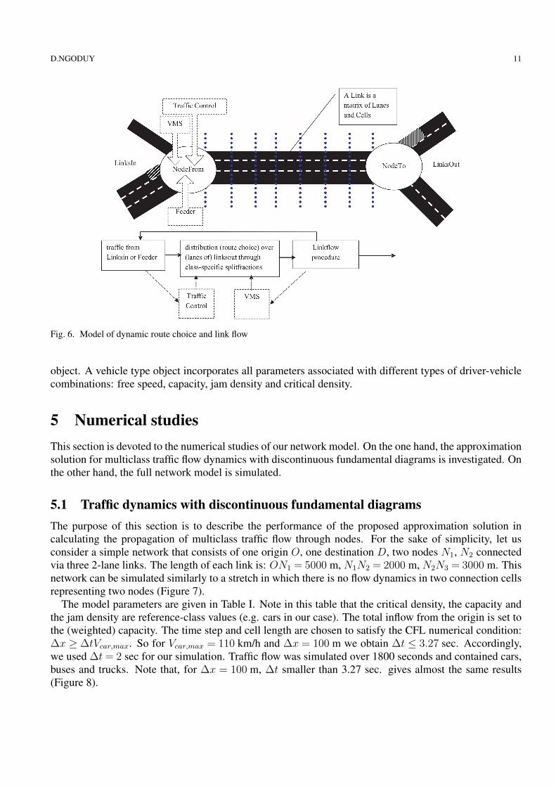
Note that simulation results with meshes finer than the chosen one almost overlap. Then, different mesheswill be used for the comparison with the assumedly analytical solution (Figure 10(a)). It is clear thatthe simulation is generally stable even for a large mesh. The deviations of numerical errors betweendifferent mesh sizes are then studied using the so-called Euclidian root mean square (RMS) error norm asin equation (24):

‖Eu(k)‖ =

√√√√1

I

I∑i=1

(rusim(i, k)− ru

exact(i, k))2. (24)

where ‖Eu(k)‖ is the class specific Euclidian RMS error norm. rusim(i,k) and ru

exact(i,k) denote, respec-tively, the class specific density at cell i and time instant k obtained from simulation and exact solution.The property of equation (24) is that if ‖Eu(k)‖ is increased in the course of time, a small initial numericalperturbation will result in large inaccuracies. Figures 10(b)-10(d) indicate that the Euclidian RMS errornorm of our simulation converges for various meshes.

14 D.NGODUY

0 2000 4000 6000 8000 100000

20

40

60

80

100

120

Location (m)

Tot

al d

ensi

ty (

veh/

km)

Numerical convergence of the model at t=600sec

analytical solutionmesh: 1.2sec&40mmesh: 2sec&100mmesh: 6sec&200mmesh: 12sec&400m

(a)

0 500 1000 1500 18000

1

2

3

4

5

6

7

8

Time (sec)

Euc

lidea

n R

MS

err

or n

orm

(ve

h/km

)

Error norm of car density

mesh:1.2sec&40mmesh:2sec&100mmesh:6sec&200mmesh:12sec&400m

(b)

0 500 1000 1500 18000

1

2

3

4

5

6

7

8

Time (sec)

Euc

lidea

n R

MS

err

or n

orm

(ve

h/km

)

Error norm of bus density

mesh:1.2sec&40mmesh:2sec&100mmesh:6sec&200mmesh:12sec&400m

(c)

0 500 1000 1500 18000

1

2

3

4

5

6

7

8

Time (sec)

Euc

lidea

n R

MS

err

or n

orm

(ve

h/km

)

Error norm of truck density

mesh:1.2sec&140mmesh:2sec&100mmesh:6sec&200mmesh:12sec&400m

(d)

Fig. 10. Numerical errors for different meshes

5.2 Full network simulation

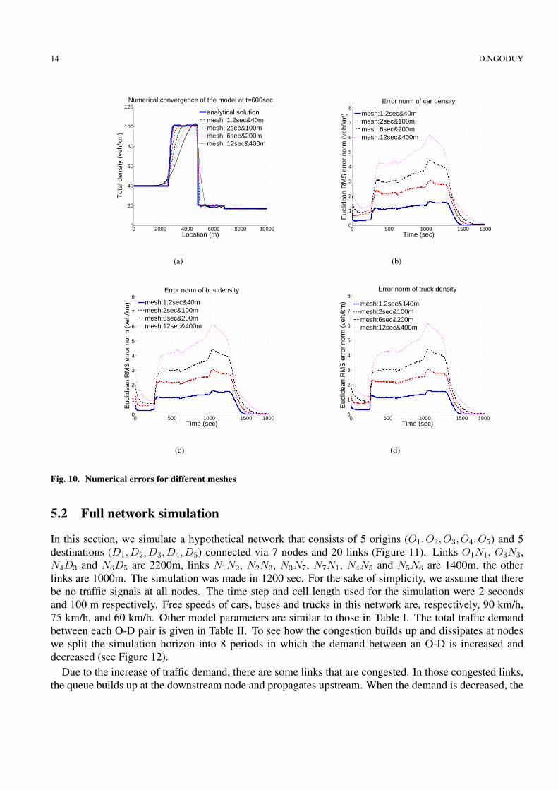
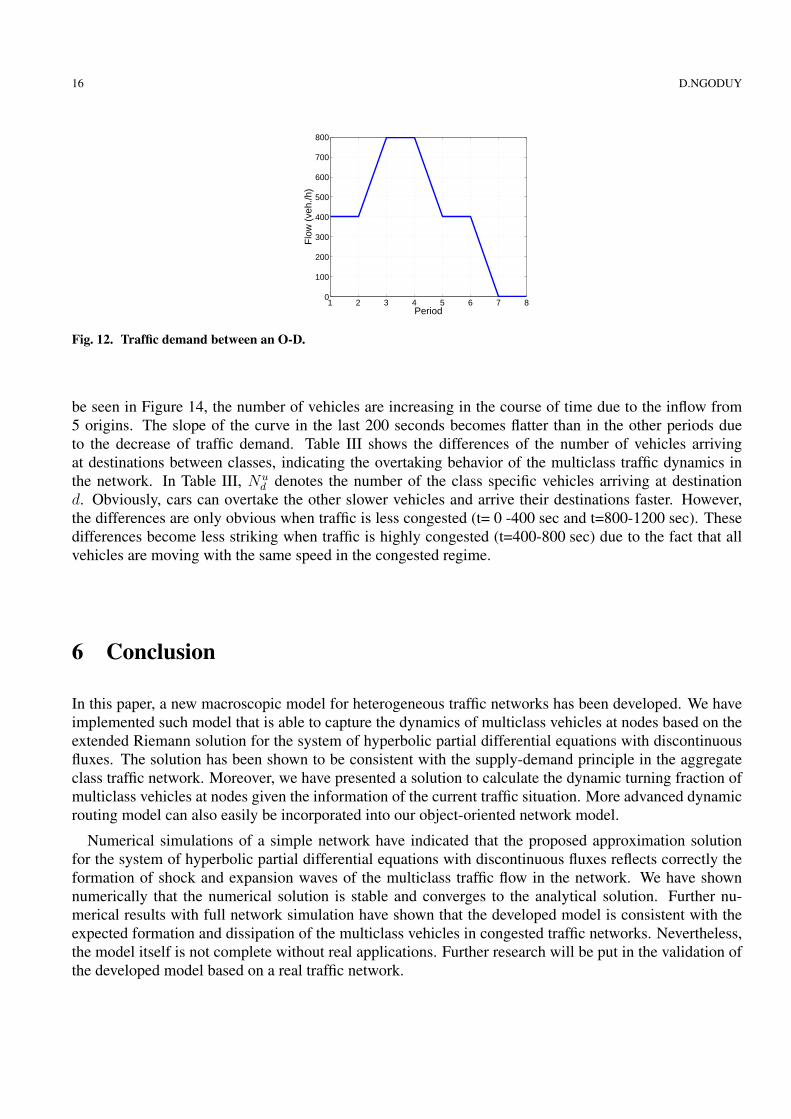
In this section, we simulate a hypothetical network that consists of 5 origins (O1,O2,O3,O4,O5) and 5destinations (D1,D2,D3,D4,D5) connected via 7 nodes and 20 links (Figure 11). Links O1N1, O3N3,N4D3 and N6D5 are 2200m, links N1N2, N2N3, N3N7, N7N1, N4N5 and N5N6 are 1400m, the otherlinks are 1000m. The simulation was made in 1200 sec. For the sake of simplicity, we assume that therebe no traffic signals at all nodes. The time step and cell length used for the simulation were 2 secondsand 100 m respectively. Free speeds of cars, buses and trucks in this network are, respectively, 90 km/h,75 km/h, and 60 km/h. Other model parameters are similar to those in Table I. The total traffic demandbetween each O-D pair is given in Table II. To see how the congestion builds up and dissipates at nodeswe split the simulation horizon into 8 periods in which the demand between an O-D is increased anddecreased (see Figure 12).

Due to the increase of traffic demand, there are some links that are congested. In those congested links,the queue builds up at the downstream node and propagates upstream. When the demand is decreased, the

D.NGODUY 15

Fig. 11. Description of the simulated network.

TABLE IIINITIAL TRAFFIC DEMAND

D1 D2 D3 D4 D5

O1 400 0 0 400 400O2 400 400 400 400 400O3 0 400 400 400 0O4 0 0 400 400 0O5 400 0 0 400 400

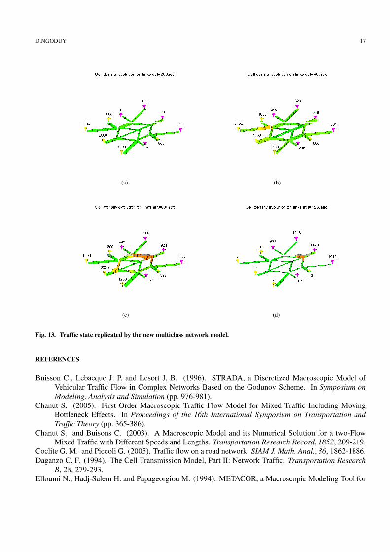
queue dissipates in the downstream direction of the link and disappears in the course of time (Figure 13).In Figure 13, the congestion level is illustrated by the color of the cells. Accordingly, green...yelllow....redcolor corresponds to the free-flow...critical...congested traffic state in each cell (the critical state is wherethe total density approaches the critical density). The total number of vehicles arriving at destinations areshown at each destination location in Figure 13. Note that these number are calculated accumulatively upto the time snap.

To verify the conservation of the number of the class specific vehicles in the simulated network, let usdetermine the following quantities:

• The number of the class specific vehicles in the network at time step k on all links:Nu(k) = ∆x

∑a

∑i r

ua(i,k).

• The number of the class specific vehicles inflowing from all origins up to time step k:Qu

in(k) = ∆t∑

o

∑kj=0 qu

o (j), where quo (j) is the class specific flow coming from origin o at time

instant j.• The number of the class specific vehicles exiting at all destinations up to time step k:

Quout(k) = ∆t

∑d

∑kj=0 q̃u

d,o(j), where q̃ud (j) is the class specific flow arriving at destination d at

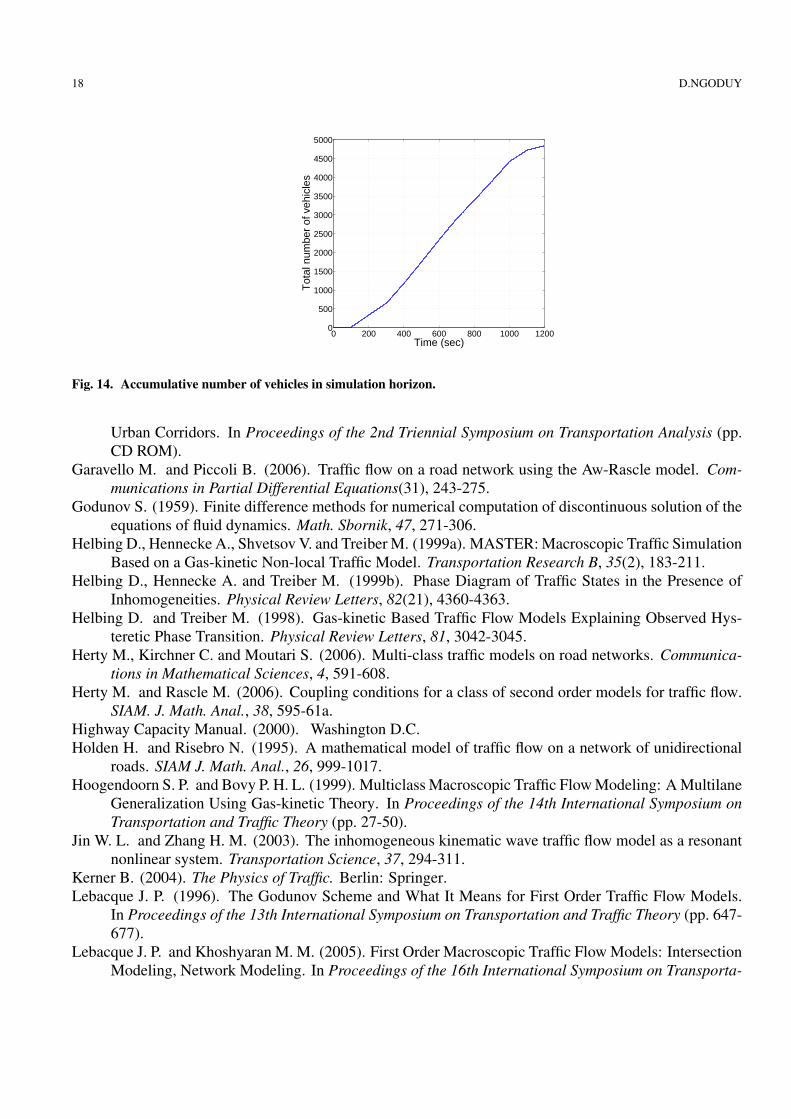
time instant j.In our simulation domain, the accumulative number of vehicles are described in Figure 14. As it can

16 D.NGODUY

1 2 3 4 5 6 7 80

100

200

300

400

500

600

700

800

PeriodF

low

(ve

h./h

)

Fig. 12. Traffic demand between an O-D.

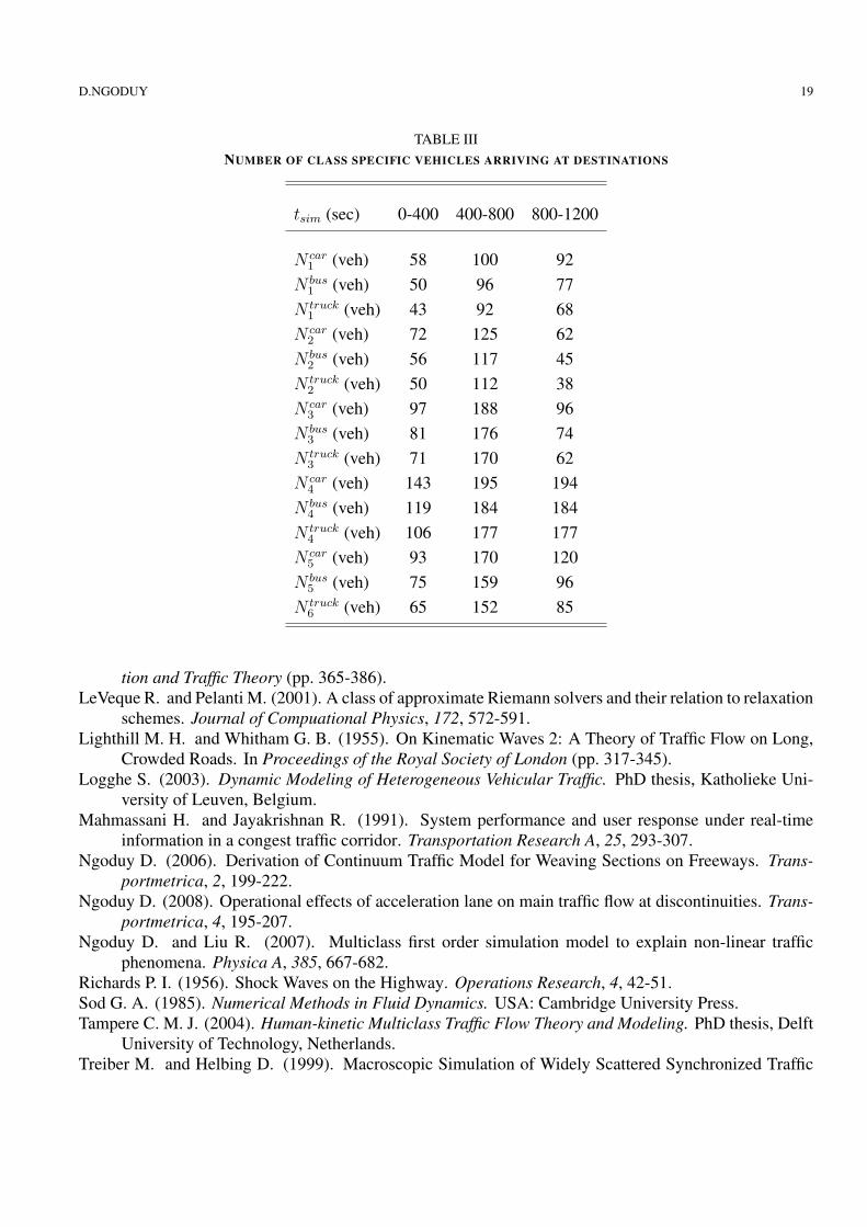
be seen in Figure 14, the number of vehicles are increasing in the course of time due to the inflow from5 origins. The slope of the curve in the last 200 seconds becomes flatter than in the other periods dueto the decrease of traffic demand. Table III shows the differences of the number of vehicles arrivingat destinations between classes, indicating the overtaking behavior of the multiclass traffic dynamics inthe network. In Table III, Nu

d denotes the number of the class specific vehicles arriving at destinationd. Obviously, cars can overtake the other slower vehicles and arrive their destinations faster. However,the differences are only obvious when traffic is less congested (t= 0 -400 sec and t=800-1200 sec). Thesedifferences become less striking when traffic is highly congested (t=400-800 sec) due to the fact that allvehicles are moving with the same speed in the congested regime.

6 Conclusion

In this paper, a new macroscopic model for heterogeneous traffic networks has been developed. We haveimplemented such model that is able to capture the dynamics of multiclass vehicles at nodes based on theextended Riemann solution for the system of hyperbolic partial differential equations with discontinuousfluxes. The solution has been shown to be consistent with the supply-demand principle in the aggregateclass traffic network. Moreover, we have presented a solution to calculate the dynamic turning fraction ofmulticlass vehicles at nodes given the information of the current traffic situation. More advanced dynamicrouting model can also easily be incorporated into our object-oriented network model.

Numerical simulations of a simple network have indicated that the proposed approximation solutionfor the system of hyperbolic partial differential equations with discontinuous fluxes reflects correctly theformation of shock and expansion waves of the multiclass traffic flow in the network. We have shownnumerically that the numerical solution is stable and converges to the analytical solution. Further nu-merical results with full network simulation have shown that the developed model is consistent with theexpected formation and dissipation of the multiclass vehicles in congested traffic networks. Nevertheless,the model itself is not complete without real applications. Further research will be put in the validation ofthe developed model based on a real traffic network.

D.NGODUY 17

(a) (b)

(c) (d)

Fig. 13. Traffic state replicated by the new multiclass network model.

REFERENCES

Buisson C., Lebacque J. P. and Lesort J. B. (1996). STRADA, a Discretized Macroscopic Model ofVehicular Traffic Flow in Complex Networks Based on the Godunov Scheme. In Symposium onModeling, Analysis and Simulation (pp. 976-981).

Chanut S. (2005). First Order Macroscopic Traffic Flow Model for Mixed Traffic Including MovingBottleneck Effects. In Proceedings of the 16th International Symposium on Transportation andTraffic Theory (pp. 365-386).

Chanut S. and Buisons C. (2003). A Macroscopic Model and its Numerical Solution for a two-FlowMixed Traffic with Different Speeds and Lengths. Transportation Research Record, 1852, 209-219.

Coclite G. M. and Piccoli G. (2005). Traffic flow on a road network. SIAM J. Math. Anal., 36, 1862-1886.Daganzo C. F. (1994). The Cell Transmission Model, Part II: Network Traffic. Transportation Research

B, 28, 279-293.Elloumi N., Hadj-Salem H. and Papageorgiou M. (1994). METACOR, a Macroscopic Modeling Tool for

18 D.NGODUY

0 200 400 600 800 1000 12000

500

1000

1500

2000

2500

3000

3500

4000

4500

5000

Time (sec)

Tot

al n

umbe

r of

veh

icle

s

Fig. 14. Accumulative number of vehicles in simulation horizon.

Urban Corridors. In Proceedings of the 2nd Triennial Symposium on Transportation Analysis (pp.CD ROM).

Garavello M. and Piccoli B. (2006). Traffic flow on a road network using the Aw-Rascle model. Com-munications in Partial Differential Equations(31), 243-275.

Godunov S. (1959). Finite difference methods for numerical computation of discontinuous solution of theequations of fluid dynamics. Math. Sbornik, 47, 271-306.

Helbing D., Hennecke A., Shvetsov V. and Treiber M. (1999a). MASTER: Macroscopic Traffic SimulationBased on a Gas-kinetic Non-local Traffic Model. Transportation Research B, 35(2), 183-211.

Helbing D., Hennecke A. and Treiber M. (1999b). Phase Diagram of Traffic States in the Presence ofInhomogeneities. Physical Review Letters, 82(21), 4360-4363.

Helbing D. and Treiber M. (1998). Gas-kinetic Based Traffic Flow Models Explaining Observed Hys-teretic Phase Transition. Physical Review Letters, 81, 3042-3045.

Herty M., Kirchner C. and Moutari S. (2006). Multi-class traffic models on road networks. Communica-tions in Mathematical Sciences, 4, 591-608.

Herty M. and Rascle M. (2006). Coupling conditions for a class of second order models for traffic flow.SIAM. J. Math. Anal., 38, 595-61a.

Highway Capacity Manual. (2000). Washington D.C.Holden H. and Risebro N. (1995). A mathematical model of traffic flow on a network of unidirectional

roads. SIAM J. Math. Anal., 26, 999-1017.Hoogendoorn S. P. and Bovy P. H. L. (1999). Multiclass Macroscopic Traffic Flow Modeling: A Multilane

Generalization Using Gas-kinetic Theory. In Proceedings of the 14th International Symposium onTransportation and Traffic Theory (pp. 27-50).

Jin W. L. and Zhang H. M. (2003). The inhomogeneous kinematic wave traffic flow model as a resonantnonlinear system. Transportation Science, 37, 294-311.

Kerner B. (2004). The Physics of Traffic. Berlin: Springer.Lebacque J. P. (1996). The Godunov Scheme and What It Means for First Order Traffic Flow Models.

In Proceedings of the 13th International Symposium on Transportation and Traffic Theory (pp. 647-677).

Lebacque J. P. and Khoshyaran M. M. (2005). First Order Macroscopic Traffic Flow Models: IntersectionModeling, Network Modeling. In Proceedings of the 16th International Symposium on Transporta-

D.NGODUY 19

TABLE IIINUMBER OF CLASS SPECIFIC VEHICLES ARRIVING AT DESTINATIONS

tsim (sec) 0-400 400-800 800-1200

N car1 (veh) 58 100 92

N bus1 (veh) 50 96 77

N truck1 (veh) 43 92 68

N car2 (veh) 72 125 62

N bus2 (veh) 56 117 45

N truck2 (veh) 50 112 38

N car3 (veh) 97 188 96

N bus3 (veh) 81 176 74

N truck3 (veh) 71 170 62

N car4 (veh) 143 195 194

N bus4 (veh) 119 184 184

N truck4 (veh) 106 177 177

N car5 (veh) 93 170 120

N bus5 (veh) 75 159 96

N truck6 (veh) 65 152 85

tion and Traffic Theory (pp. 365-386).LeVeque R. and Pelanti M. (2001). A class of approximate Riemann solvers and their relation to relaxation

schemes. Journal of Compuational Physics, 172, 572-591.Lighthill M. H. and Whitham G. B. (1955). On Kinematic Waves 2: A Theory of Traffic Flow on Long,

Crowded Roads. In Proceedings of the Royal Society of London (pp. 317-345).Logghe S. (2003). Dynamic Modeling of Heterogeneous Vehicular Traffic. PhD thesis, Katholieke Uni-

versity of Leuven, Belgium.Mahmassani H. and Jayakrishnan R. (1991). System performance and user response under real-time

information in a congest traffic corridor. Transportation Research A, 25, 293-307.Ngoduy D. (2006). Derivation of Continuum Traffic Model for Weaving Sections on Freeways. Trans-

portmetrica, 2, 199-222.Ngoduy D. (2008). Operational effects of acceleration lane on main traffic flow at discontinuities. Trans-

portmetrica, 4, 195-207.Ngoduy D. and Liu R. (2007). Multiclass first order simulation model to explain non-linear traffic

phenomena. Physica A, 385, 667-682.Richards P. I. (1956). Shock Waves on the Highway. Operations Research, 4, 42-51.Sod G. A. (1985). Numerical Methods in Fluid Dynamics. USA: Cambridge University Press.Tampere C. M. J. (2004). Human-kinetic Multiclass Traffic Flow Theory and Modeling. PhD thesis, Delft

University of Technology, Netherlands.Treiber M. and Helbing D. (1999). Macroscopic Simulation of Widely Scattered Synchronized Traffic

20 D.NGODUY

States. Journal of Physics A: Mathematical and General, 59, 239-253.Wong G. C. K. and Wong S. C. (2002). A Multiclass Traffic Flow Model-an Extension of LWR Model

with Heterogeneous Drivers. Transportation Research A, 36, 763-848.Zhang P., Liu R. X., Wong S. C. and Dai S. Q. (2006a). Hyperbolicity and Kinematic Waves of a Class

of Multi-population Partial Differential Equations. European Journal of Applied Mathematics, 17,171-200.

Zhang P., Wong S. C. and Shu C. W. (2006b). A weighted essentially non-oscillatory numerical scheme fora multi-class traffic flow model on an inhomogeneous highway. Journal of Computational Physics,212, 739-756.

Zhang P., Wong S. C. and Xu Z. L. (2008). A hybrid scheme for solving a multi-class traffic flow withcomplex wave breaking. Computer Methods in Applied Mechanics and Engineering, 197, 3816-3827.