National Aeronautics andSpace Administration

Langley Research CenterHampton, Virginia 23681-2199

NASA/CR-2000-210543ICASE Report No. 2000-37

Discontinuous Dual-primal Mixed Finite Elements forElliptic Problems

Carlo L. Bottasso, Stefano Micheletti, and Riccardo SaccoPolitecnico di Milano, Milano, Italy

ICASENASA Langley Research CenterHampton, Virginia

Operated by Universities Space Research Association

October 2000

Prepared for Langley Research Centerunder Contract NAS1-97046

DISCONTINUOUS DUAL-PRIMAL MIXED FINITE ELEMENTS FOR ELLIPTIC

PROBLEMS

CARLO L. BOTTASSO�, STEFANO MICHELETTIy, AND RICCARDO SACCOz

Abstract. We propose a novel discontinuous mixed �nite element formulation for the solution of

second-order elliptic problems. Fully discontinuous piecewise polynomial �nite element spaces are used

for the trial and test functions. The discontinuous nature of the test functions at the element interfaces

allows to introduce new boundary unknowns that, on the one hand enforce the weak continuity of the

trial functions, and on the other avoid the need to de�ne a priori algorithmic uxes as in standard

discontinuous Galerkin methods. Static condensation is performed at the element level, leading to a

solution procedure based on the sole interface unknowns.

The resulting family of discontinuous dual-primal mixed �nite element methods is presented in the

one and two-dimensional cases. In the one-dimensional case, we show the equivalence of the method

with implicit Runge-Kutta schemes of the collocation type exhibiting optimal behavior. Numerical

experiments in one and two dimensions demonstrate the order accuracy of the new method, con�rming

the results of the analysis.

Subject classi�cation. Applied and Numerical Mathematics

Key words. �nite element method, mixed methods, discontinuous Galerkin, Petrov-Galerkin,

elliptic problem

1. Introduction and Motivation. We consider the following classical model problem:

(�div(�ru) = f in � R

2;

u = g on @;(1.1)

where is a bounded polygon with Lipschitz boundary � = @, and �, f , g are given functions.

Dirichlet boundary conditions are considered only for the sake of simplicity, but the extension to

the case of more general boundary data is straightforward. De�nitions of functional and geometrical

entities are given in section 2.

In view of the approximation of (1.1), we let fThgh>0 be a family of triangulations of and, for

any Th, we denote by T any element thereof. Introducing the auxiliary unknown � = �r u, problem

�Dipartimento di Ingegneria Aerospaziale, Politecnico di Milano, Via La Masa 34, 20158 Milano, Italy (email:

Carlo.Bottasso@polimi.it). This research was supported by the National Aeronautics and Space Administration under

NASA Contract No. NAS1-97046 while the �rst author was in residence at ICASE, NASA Langley Research Center,

Hampton, VA 23681-2199.yDipartimento di Matematica \F. Brioschi", Politecnico di Milano, Via Bonardi 9, 20133 Milano, Italy (email:

Stefano.Micheletti@polimi.it).zDipartimento di Matematica \F. Brioschi", Politecnico di Milano, Via Bonardi 9, 20133 Milano, Italy (email:

Riccardo.Sacco@polimi.it).

1

(1.1) can be reformulated in weak form over each element T of Th as8><>:ZT

��1

� � � dx+

ZT

u div� dx�

Z@T

u � � nT ds = 0;ZT

� � r v dx�

Z@T

v � � nT ds =

ZT

fv dx;

(1.2)

where � and v are smooth vector and scalar functions, respectively, on T , while nT is the unit outward

normal vector to @T .

A uni�ed framework for the analysis of the Discontinuous Galerkin (DG) method applied to elliptic

problems in the form (1.2) was provided in ref. [1]. We shall follow the same path in the following,

since the proposed method �ts well in that framework. The DG formulation at the discrete level reads

(see also [9]): �nd uh 2 Uh and �h 2 �h such that 8T 2 Th8>>><>>>:

ZT

��1

�h � �h dx+

ZT

uh div�h dx�Xe2@T

Ze

hu�h � nT ds = 0 8�h 2 �(T );ZT

�h � r vh dx�

Xe2@T

Ze

vhh� � nT ds =

ZT

fvh dx 8vh 2 U(T );(1.3)

where �(T ) and U(T ) are two sets of smooth vector and scalar functions, typically polynomials, de�ned

on each element T , while �h and Uh are the corresponding global �nite element spaces. We are now

dealing with a Galerkin method where the values of the unknown �elds on each edge e of @T , noted

uhje and �hje, have been replaced by the numerical uxes hu and h�. In practical implementations,

hu and h� are chosen as functions of the internal unknowns uh and �h on two neighboring triangles.

In particular, it can be shown that most methods reported in the literature can be classi�ed based on

the particular choice of the numerical uxes hu and h� , choice often inspired by ideas borrowed from

�nite volume methods. The interested reader can consult ref. [1] for exact details on the expressions

of the uxes in the di�erent cases.

It is clear that any particular choice on the nature of the numerical uxes will a�ect the resulting

scheme, eventually determining its numerical characteristics, stability, accuracy as well as the pattern

of the sti�ness matrix. This approach to the choice of the numerical uxes is somewhat unsatisfactory,

in the sense that it seems to be a rather arti�cial and dogmatic process, in some sense a \violence"

to the underlying weak form (1.2). In this work, we shall therefore depart from the classical approach

of de�ning a priori the expressions of the numerical uxes. Hence, the interface �elds hu and h� � nT

are assumed to represent new additional problem unknowns, and we let the method implicitly de�ne

their values. In doing so, we obtain a genuine Petrov-Galerkin version of the DG method.

This formulation generalizes the method described in refs. [2, 3, 4, 5] to multiple spatial dimen-

sions. In the one-dimensional case, the method can be shown to be equivalent to collocation-type

implicit Runge-Kutta (RK) schemes. In particular, when used in conjunction with Gauss-Legendre

quadrature, the �nite element method here proposed corresponds to the Kuntzmann-Butcher (Gauss)

RK scheme, which enjoys well known properties of optimality. This provides a strong motivation for

seeking an extension of those ideas to the multi-dimensional case, extension that is attempted in this

work for the elliptic boundary-value problem.

The paper is laid out as follows. Section 2 presents the proposed method for the classical problem

of the Laplacian. Section 3 deals with the one-dimensional formulation of the present method and

2

with its connections with the time �nite element and RK methods of refs. [2, 3, 4, 5]. In doing so,

we shall temporarily abandon the simple linear model problem, and present the method for a general

non-linear ODE problem. Section 4 is devoted to the description of the method in the two-dimensional

case. Numerical results are discussed in section 5, where the proposed method is validated on one and

two-dimensional test cases. Finally, the conclusions are discussed in section 6.

2. The Discontinuous Dual-Primal Mixed Method for a Model Problem. We are now

ready to de�ne the proposed Discontinuous Dual-Primal Mixed (DDPM) discretization of the one-

element weak formulation of problem (1.1): �nd uh 2 Uh, �h 2 �h, �h 2 �h;g and �h 2 �h such that

8T 2 Th we have8><>:ZT

��1�h � �h dx+

ZT

uh div�h dx�

Z@T

�h�h � nT ds = 0 8�h 2 W (T );ZT

�h � r vh dx�

Z@T

ST vh�h ds =

ZT

fvh dx 8vh 2 V (T ):(2.1)

The meaning of the symbols is as follows. For any Th 2 fThgh>0, let Eh be the associated set of

edges. For any edge e of Eh, we denote by ne the unit normal vector to e, directed according to a

uniquely �xed arbitrary convention. Namely, ne coincides with the unit outward normal vector on the

boundary � if e \ � 6= ;, otherwise ne coincides with one of the two outward normals to the triangles

sharing the edge e if e\� = ;. Then, for any T 2 Th we denote by nT the unit outward normal vector

to @T and de�ne the sign function ST = ne � nT = �1. Through the use of ST , we can associate the

interface degrees of freedom with mesh edges, so that the sign function will determine whether a given

ux �h is entering of exiting from a given triangle. For simplicity, we shall omit in the following the

dependence of n on the edge e which will be understood.

Given the fact that the edge uxes are now unknowns to the problem, we can not choose test and

trial functions within the same spaces, as for the DG method (1.3). Therefore, we are now dealing

with a Petrov-Galerkin formulation. The global �nite element spaces for the internal variables �h and

uh are de�ned as

�h =�vh 2 L

2() j vhjT 2 �(T )8T 2 Th

;

Uh =�vh 2 L

2() j vhjT 2 U(T )8T 2 Th

;

where L2() = (L2())2. Considering now the interface �elds �h and �h, we note that they represent

the traces of u and � � nT on @T , respectively. Using the language of computational mechanics, the

new unknowns act as \mixed connectors" between neighboring triangles (see [16] and [18], Chapter

13). We let �(e) indicate a set of scalar smooth functions de�ned on each edge e. Then, we de�ne the

(global) �nite dimensional spaces

�h =��h 2 L

2(Eh) j �hje 2 �(e)8e 2 Eh

;

�h;g = f�h 2 �h j �h = Pg if e \ � 6= ;g ;

where P is the L2-projection operator on �(e). Finally, we introduce the local and global �nite element

spaces for the test functions � and v. Denoting by W (T ) and V (T ) two sets of smooth vector and

3

scalar functions de�ned on each element T , we have

W h =��h 2 L

2() j �hjT 2W (T )8T 2 Th

;

Vh =�wh 2 L

2() jwhjT 2 V (T )8T 2 Th

:

The choice of the functional spaces will be detailed in the following sections for the one and the

two-dimensional case.

We note that the method is completely conservative in the sense of ref. [1], since the interface

unknowns are associated with edges and are consequently identical for two triangles sharing the edge.

This last property implies the following conservation statementXe2@U

Ze

�h ds+

ZU

f dx = 0;

where U is the union of some collection of elements, and vh was taken to be identically unity in the

second of (2.1).

The DDPM approach can be viewed as a consistent hybridization of the dual-primal mixed (DPM)

method introduced in ref. [12]. Indeed, the spirit of the standard hybridization procedure (see [7],

Chapter V) is to relax the continuity of some of the unknowns (� � n in the dual hybrid philosophy or

u in the primal hybrid philosophy) and then to enforce it back through the introduction of suitable

inter-element Lagrange multipliers. Precisely, uje represents the Lagrange multiplier in the case of

dual hybrid methods, while � � nje is the Lagrange multiplier in the case of primal hybrid methods.

In the present case, we relax the continuity of both u and � � n in the interior �elds and let the

interface variables connect neighboring elements. The interface variables � and � do not play the

role of Lagrange multipliers in our case but, nevertheless, enjoy appealing properties. Physically, they

have the clear meaning of uje and � � nje, respectively, while numerically they exhibit a higher rate of

convergence than the internal variables, as it will be shown in the following. This is also a feature of

the Lagrange multipliers in the case of standard hybrid methods ([7], Chapter V).

Alternatively, one could note that, by gluing the test functions together at neighboring triangles,

each internal edge receives equal and opposite contributions from the two elements using it, and

therefore the boundary unknowns are eliminated. This way one recovers from (2.1) the DPM method.

3. The DDPM Method in the One-Dimensional Case. We abandon now for the moment

the linear model problem (1.1), and we consider a generic system of �rst order ODE's

z0 = f(z; x); (3.1)

where z; f 2 RD

and D is the number of state variables. Suitable initial or two-point boundary

conditions complement problem (3.1). In the case of the linear model problem, we clearly have

z = (u; �)T and f = (�;�f)T . However, since the discussion can be easily completed for the more

general case, we consider (3.1) instead of the one-dimensional version of (1.1) in the remainder of this

section.

We assume = (0; X) and let 0 � x0 < x1 < : : : < xn�1 < xn � X be a given partition Th of

into n � 1 intervals Ti = [xi; xi+1] of size hi, i = 0; : : : ; n � 1, where fxigni=0 are the nodes. Note

that in the one-dimensional case Eh � fxigni=0 and each edge e degenerates into one single node.

4

The statement of the present �nite element method is as follows: �nd (zh; �h) 2 (Zh � �h) such

that for each Ti 2 Th, i = 0; : : : ; n� 1, the following holds

ZTi

zh � w0

h dx+

ZTi

f(zh; x) � wh dx� (�i+1 � wh(xi+1)� �i � wh(xi)) = 0

8wh 2W (Ti): (3.2)

For any T 2 Th, we de�ne the local �nite element spaces for the internal �elds zh and for the test

functions as follows:

Z(T ) = (Pk(T ))D; W (T ) = (Pk+1(T ))

D;

with k � 0. The local �nite element space for the interface unknowns �h is

�(@Ti) = f�i; �i+1g; i = 0; : : : ; n� 1;

where for any function � 2 �(@Ti) we let �i = �(xi) and �i+1 = �(xi+1), i = 0; : : : ; n�1. Furthermore,

we set

U(T ) = U(T )� �(@T ); V(T ) = W (T ):

The �nite element space is then

D Pk(T ) = f(z; �;w) j (z; �;w) 2 U(T )� V(T )8T 2 Thg: (3.3)

The global �nite element spaces for the internal �elds and the test functions are

Zh =�zh 2 (L2())D j zhjT 2 Z(T )8T 2 Th

;

W h =�wh 2 (L2())D jwhjT 2 W (T )8T 2 Th

;

while the global spaces for the interface unknowns are

�h =nf�ig

ni=0 j�i 2 R

D; i = 0; : : : ; n

o;

where functions are de�ned only at the nodes of Eh. Finally, gathering the previous de�nitions, we

obtain the global �nite element space as

D Pk

h = (Zh � �h)�W h: (3.4)

It is clear that both initial and boundary-value problems can be solved within this framework.

For an initial value problem, one can solve marching sequentially in an element-by-element fashion, as

with any time stepping procedure. We have: dim(Z(T )) = D(k+1), dim(W (T )) = D(k+2) 8T 2 Th.

Therefore, for any T 2 Th, (3.2) leads to a system of D(k + 2) equations in the D(k + 1) + 2D

local unknowns zhjT , �hjT , leaving space for the D initial conditions that complement problem (3.1).

A boundary-value problem leads to a global discrete problem de�ned over . In this case we have

nD(k+2) equations in the nD(k+1)+2nD unknowns. However, considering that �i+1 appears in both

neighboring elements Ti and Ti+1, the total unknown count is reduced to nD(k+1)+2nD� (n�1)D,

5

which leaves once again space for D two-point boundary values. In both cases, the internal �eld zh

can be eliminated at the element level in favor of the interface unknowns �h, and then recovered at

convergence.

We note that the scheme presents two jump discontinuities for each �nite element, namely one at

xi and the other at xi+1, since �i 6= zh(xi) and �i+1 6= zh(xi+1). For this reason it was termed the

Bi-Discontinuous (BD) scheme in ref. [3]. It is clear that such symmetric treatment of the element

boundaries implies no privilege in the direction of the ow of information, and it is therefore best

suited for two-point boundary-value problems.

Quite di�erently, for initial value problems it is sometimes desirable to have sti�y accurate

schemes, that are able to damp the higher frequencies components from the computed response [11].

This is achieved in practice by forcing a lack of symmetry in the scheme, that incorporates the knowl-

edge on the direction of ow of information within the element. It is possible to derive such schemes

in the present framework, allowing one single jump discontinuity at xi while enforcing the condition

�i+1 = zh(xi+1). One obtains in this case the so called Singly-Discontinuous (SD) schemes [3].

3.1. Equivalence with Runge-Kutta Methods. It was shown in ref. [3] and then again with

a slightly di�erent proof in ref. [4], that the �nite element method (3.2) can be written as a RK process

for any order k. RK methods are probably best known for the solution of initial value problems, but

clearly can also be used for the solution of two-point boundary-value problems by assembling the

single steps to yield a global discrete problem de�ned over the whole computational domain, exactly

as in the �nite element method. Since the link between the two approaches seems to be useful in the

characterization of the proposed method, we brie y review this result in the following.

We begin by selecting a quadrature rule for the evaluation of the integrals in (3.2). The rule is

de�ned by s absciss� ci and weights bi. We consider the case s = k + 1, therefore the number of

quadrature points is the same as the number of �nite element nodes of the trial functions.

Following the usual FEM practice, one expresses the discrete equations in terms of the nodal

values. Here we shall take a di�erent approach, and assume as unknowns the values of the �nite

element trial functions at the quadrature points. This is the key idea for showing the link existing

between �nite element and RK methods. The change of unknowns can be done because we are using

a quadrature rule that uses as many integration points as the number of �nite element nodes, as

previously said. We will come back later to some interesting consequences of this assumption.

We �rst note that the test functions can be expressed as

wh =

k+2Xi=1

�i�1

�i; (3.5)

where � j are polynomials, � 2 R , and �k their associated amplitudes. Next, let us de�ne the (s+1)�s

matrix P� =��i�1

j�=�j

�, with i = 1; : : : ; s+1, j = 1; : : : ; s, the �j 's being s real values. The derivative

of P� with respect to � is then P0

� =�(i� 1)� i�2j�=�j

�. Note that, for any choice of the �j 's, the �rst

row of P� is all made of one's, and the �rst row of P 0

� is all made of zero's. For �j = cj , we have the

matrices Pc =�ci�1j

�, P 0

c =�(i� 1)ci�2j

�. We also de�ne the s� s diagonal matrix B =

h-

bi&

i, with

i = 1; : : : ; s, and the following s-dimensional vectors: b = (b1; b2; : : : ; bs)T , c = (c1; c2; : : : ; cs)

T , and

6

0 = (0; 0; : : : ; 0)T , 1 = (1; 1; : : : ; 1)T , 11 = (1; 0; : : : ; 0)T .

We note that

P0

cB =

"0T

Q0

#; (3.6)

Q being the s� s matrix Q =��ij�=cjbj

�=

�cijbj

�. The derivative of Q with respect to � is given by

Q0 =

�i c

i�1j bj

�. Furthermore, if the quadrature formula is of order s, we have that

Q01 = 1: (3.7)

Equation (3.7) corresponds to the so called \B simplifying assumption" in the theory of RK methods.

The discrete weak form (3.2) can now be written as

((P 0

cB) ID) z + hi((PcB) ID) f = (1 ID)�i+1 � (11 ID)�i; (3.8)

where the following two sD-dimensional vectors were de�ned: z = (z1; : : : ; zs)T , f = (f(z1; xi +

c1hi); : : : ; f(zs; xi + cshi))

T . ID is the D �D identity matrix, while denotes the tensor Kronecker

product of matrices, so that (�) ID ensures that all degrees of freedom of the vectorial problem are

integrated according to the same rule.

Solving for z and �i+1 and using (3.7), we have

(z; �i+1)T =

"1 hi(1b

T�Q

0�1

Q)

1 hibT

# ID(�i; f)

T: (3.9)

From this expression, we conclude that (3.2) can be written as a s-stage RK method whose tableau

[10] is given by

c 1bT �Q0�1

Q

bT

: (3.10)

Finally, we test the Gauss-Legendre, Lobatto and Radau quadrature rules and compute the cor-

responding tableaux (3.10). The results are summarized in Table (3.1).

Table 3.1

Correspondence between quadrature rules for BD �nite elements and RK methods.

Quadrature Rule RK Method

Gauss Kuntzmann-Butcher

Lobatto Lobatto IIIB

Radau-Left Radau IA

Table (3.1) shows that the family of schemes deriving from the one-dimensional �nite element

method considered in this work corresponds to some well known RK algorithms. The two approaches

di�er on the choice of the unknowns: the �nite element method solves for the nodal values, while

7

the RK method solves for the quadrature point values. However, these two sets of values are simply

related by a linear transformation. Furthermore, note that all RK schemes appearing in the table

are of the collocation type, where polynomials interpolate the two interface values �i, �i+1 and the

internal stages z [10]. This link between �nite elements and RK processes allows a somewhat unique

way of looking at the discretization procedure: from the �nite element point of view we see jumps

in the �eld variables, since we have discontinuous interpolations of the internal �elds, glued together

from one element to its neighbor through the presence of the interface unknowns. Quite di�erently,

from the RK point of view we have continuous interpolations of the interface unknowns with internal

variables at the collocation points, with apparently no jump discontinuities in the solution. It should

also be remarked that for these RK methods, maximal order is in general attained only at the interface

values, and not at the internal stages. We then expect to observe higher rates of convergence of the

interface �elds also in the multi-dimensional generalization of the method.

The same table shows that the present �nite element formulation, when used in conjunction

with Gauss-Legendre quadrature, yields the Kuntzmann-Butcher (or Gauss) RK methods. These RK

schemes are probably the ones that enjoy the greatest number of numerical properties, and are in

this sense optimal. In fact they are of maximal order (2s), they are algebraically stable, and also

symplectic when applied to Hamiltonian systems [17]. Simplecticity is the distinguishing property of

Hamiltonian systems, and its numerical preservation has a strong in uence on the behavior of the

integration scheme.

As a �nal point, we note that these results are solely based on having assumed a quadrature rule

that uses as many points as the number of �nite element nodes. In reality, working from the point

of view of the �nite element method, one could choose to use a greater number of quadrature points,

for example in the hope of improving the accuracy in the evaluation of strongly non-linear functions

in the term

ZTi

f(zh; x) � wh dx. It can be shown however, that increasing the number of quadrature

points can in reality degrade the performance of the method. For example, using a larger number of

points destroys the symplectic nature of the scheme [3].

4. The Two-Dimensional Case. For two spatial dimensions, the choice of the �nite element

spaces for the internal and interface unknowns is a straightforward extension of those introduced in

the one-dimensional case. Precisely, for k � 0 we set

�(T ) =�Pk(T )

�2; U(T ) = Pk(T ) 8T 2 Th;

�(e) = Pk(e) 8e 2 Eh:

The choice of the �nite element test spaces is less obvious and requires some care. Here we

focus on the description of the method in the cases k = 0 and k = 1. We start by introducing the

Raviart-Thomas �nite element space of degree k [14]

RTk(T ) =�Pk(T )

�2� xPk(T ) 8T 2 Th:

In the case of the D P0

h �nite elements, we set W (T ) = RT0(T ) and V (T ) = P1(T ). The global �nite

element spaces W h and Vh are then simply de�ned as the products of the corresponding local spaces.

8

Notice that W h and Vh are the discontinuous counterparts of the corresponding test spaces that have

been used in the dual-primal formulation of ref. [12].

In the case of the D P1

h �nite elements, we set W (T ) = RT1(T ) and V (T ) = P2(T )� B3(T ) for

each T 2 Th. B3(T ) is the following cubic bubble [15]

B3 = ('0 � '1)('1 � '2)('2 � '0);

where 'i = 'i(x), i = 0; 1; 2, are the centroidal coordinates of a point x 2 R2with respect to the

vertices of T . Enrichment of the scalar test space is a standard procedure in hybrid methods when

the degree of the polynomials in V (T ) is even (see refs. [15, 8]). Actually, one can check that without

adding the cubic bubble the rectangular matrix arising from the integral

Z@T

ST vh�h ds becomes rank

de�cient.

As far as the implementation is concerned, we point out that for both the k = 0 and k = 1 cases

it is possible to perform a static condensation of the internal variables in favor of the edge unknowns,

obtaining a linear system in the sole interface variables �h and �h.

The generalization of the DDPM method to higher orders will be more extensively addressed in a

forthcoming paper. Let us just mention that a possible general recipe for constructing the D Pkh �nite

element spaces for even k can be given as

W (T ) = BDFMk+1(T ); V (T ) = Pk+1(T ) 8T 2 Th;

where BDFMk+1 is the triangular analogue of the reduced element introduced in ref. [6].

5. Numerical Results. In this section we demonstrate the D Pkh �nite elements for k = 0 and

k = 1 through the solution of test cases in both one and two spatial dimensions.

5.1. One-Dimensional Examples. We consider the following two-point boundary-value model

problem (�(�(x)u0(x))0 = f(x); 0 < x < 1;

u(0) = u(1) = 0:(5.1)

In all numerical experiments, successively �ner uniform grids of size h = 2�j , j 2 f1; : : : ; 9g are used.

We set eu = u � uh and e� = � � �h; moreover e� and e� denote the functions de�ned only at the

nodes of Eh such that e�(xi) = u(xi)� �i and e�(xi) = �(xi)� �i, i = 0; : : : ; n.

For any function v 2 L2() and su�ciently smooth on each T 2 Th, we denote by I1;T (v) the

approximation ofRTv dx using the trapezoidal rule. Moreover, for each T 2 Th we denote by fx

kj;T g

kj=0

the k + 1 Gauss-Legendre points on T . In order to measure the convergence rate of the D Pk

h �nite

elements, we use the following three norms:

kvkh;0; =

n�1Xi=0

I1;Ti(v2)

!1=2;

kwkh;GP;1 =

8><>:

maxi2f0;��� ;n�1g

jw(x00;T ))j; if k = 0;

maxi2f0;��� ;n�1g

�max

j2f0;1g(jw(x1j;T )j)

�; if k = 1;

k�kh;1 = maxi2f0;��� ;ng

j�ij;

9

where w is any bounded function de�ned at the Gauss points of Th and � is any bounded function

de�ned at the nodes of Th. Clearly, k � kh;0; is a discrete L2() norm, while the other two norms are

discrete maximum norms over the set of Gauss points and Eh, respectively. The quadrature formula

used in the discrete norm is accurate enough not to pollute the computed accuracy, and at the same

time avoids to sample the solution at superconvergent points. Moreover, observe that any integral

appearing in the DDPM discretization of (5.1) has been computed using a one-point Gauss-Legendre

quadrature rule (with node x00 on each T 2 Th) for k = 0 and a two-point Gauss-Legendre quadrature

rule (with nodes fx1j;T g1j=0 on each T 2 Th) for k = 1.

The following symbols are used in the graphs: for any h, symbol `*' refers to keukh;0; (or

ke�kh;0;), while symbols `�' and `o' denote keukh;GP;1 (or ke�kh;GP;1) and ke�kh;1 (or ke�kh;1),

respectively.

Test Case 1 We set �(x) = 1 and f(x) = sin(�x), x 2 [0; 1]. The exact solution is the smooth

function u(x) = (1=�2) sin(�x), which implies �(x) = u0(x) = (1=�) cos(�x). We show in �gure 5.1

the error curves for eu and e� (left) and e� and e� (right) in the case k = 0. The corresponding error

curves in the case k = 1 are shown in �gure 5.2.

10−3

10−2

10−1

100

10−8

10−6

10−4

10−2

100

1

2

10−3

10−2

10−1

100

10−8

10−6

10−4

10−2

100

1

2

Fig. 5.1. One spatial dimensions, test case 1. Approximation errors eu and e� (left) and e� and e� (right) for

D P0

h �nite elements.

The plots show second-order convergence for the interface unknowns in the case k = 0, while the

internal unknowns are only �rst-order accurate. Superconvergence of the internal variables can be

observed at the Gauss point. For the D P1

h �nite elements, the error curves show that the interface

unknowns are fourth-order convergent, the internal �elds are second-order accurate while a third-order

convergence rate is exhibited by the internal unknowns at the two Gauss points of each element. All

these results are in agreement with the theory of RK methods.

10

10−3

10−2

10−1

100

10−15

10−10

10−5

100

23

4

10−3

10−2

10−1

100

10−15

10−10

10−5

100

23

4

Fig. 5.2. One spatial dimensions, test case 1. Approximation errors eu and e� (left) and e� and e� (right) for

D P1

h�nite elements.

Test Case 2 This test problem demonstrates the performances of the DDPM method in the presence

of strong solution gradients. The coe�cient � and the source term f are chosen as in ref. [13] (see

also ref. [8], section 4.4.1, for further comments), and read

�(x) =1

�+ �(x � x)2;

f(x) = 2�1 + �(x � x)

�tan�1(�(x � x)) + tan�1(�x)

�:

The exact solution is

u(x) = (1� x)�tan�1(�(x � x)) + tan�1(�x)

�;

�(x) =

�1

�+ �(x� x)2

��� tan�1(�(x � x))� tan�1(�x) + (1� x)

�

1 + �2(x� x)2

�;

where �(x) = �(x)u0(x). Furthermore, we set � = 100 and x = 0:36388.

We show in �gure 5.3 the error curves for eu and e� (left) and e� and e� (right) in the case k = 0.

The corresponding error curves in the case k = 1 are shown in �gure 5.4.

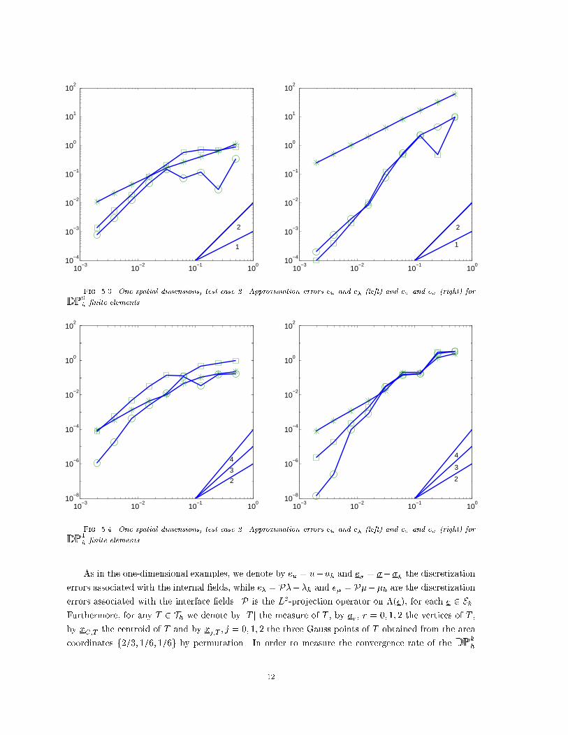
The numerical results clearly show the increased \roughness" of the problem when compared

with the corresponding error curves for test case 1. Nevertheless, all variables attain the expected

convergence rate as h! 0. Figure 5.5 shows the exact solution u (solid line) plotted against the �nite

element solution �h computed with D P0

h elements and h = 1=20. Notice the sharp internal layer,

resolved within one element.

5.2. Two-Dimensional Examples. For the two-dimensional case, we consider (1.1) in the

square domain = (�1; 1)2 with g = 0. The exact solution is in this case u(x; y) = (x2�1)(y2�1) and

�(x; y) = 2�x(y2 � 1); y(x2 � 1)

�T; the right-hand side f is computed accordingly. In all numerical

experiments, we use a uniform grid of isosceles right triangles of size hx = hy = h, where h takes on

the values 21�j=5, j 2 f0; 1; 2; 3g for the D P0

h case and f2=5; 2=10; 2=20; 2=30g for the D P1

h case.

11

10−3

10−2

10−1

100

10−4

10−3

10−2

10−1

100

101

102

1

2

10−3

10−2

10−1

100

10−4

10−3

10−2

10−1

100

101

102

1

2

Fig. 5.3. One spatial dimensions, test case 2. Approximation errors eu and e� (left) and e� and e� (right) for

D P0

h �nite elements.

10−3

10−2

10−1

100

10−8

10−6

10−4

10−2

100

102

2

3

4

10−3

10−2

10−1

100

10−8

10−6

10−4

10−2

100

102

2

3

4

Fig. 5.4. One spatial dimensions, test case 2. Approximation errors eu and e� (left) and e� and e� (right) for

D P1

h�nite elements.

As in the one-dimensional examples, we denote by eu = u�uh and e� = ���h the discretization

errors associated with the internal �elds, while e� = P���h and e� = P���h are the discretization

errors associated with the interface �elds. P is the L2-projection operator on �(e), for each e 2 Eh.

Furthermore, for any T 2 Th we denote by jT j the measure of T , by ar, r = 0; 1; 2 the vertices of T ,

by xC;T the centroid of T and by xj;T ; j = 0; 1; 2 the three Gauss points of T obtained from the area

coordinates f2=3; 1=6; 1=6g by permutation. In order to measure the convergence rate of the D Pkh

12

0 0.2 0.4 0.6 0.8 10

0.2

0.4

0.6

0.8

1

1.2

1.4

1.6

1.8

Fig. 5.5. One spatial dimensions, test case 2. Exact solution (solid line) and numerical solution �h (`o') computed

using D P0

h �nite elements (h = 1=20).

�nite elements, we introduce the following discrete norms:

kvkh;0; =

XT2Th

jT j

3

2Xr=0

(v(ar))2

!1=2

;

kvkh;GP;1 =

8<:

maxT2Th

jv(xC;T )j; if k = 0;

maxT2Th

maxj2f0;1;2g

jv(xj;T )j; if k = 1;

k�kh;�1=2;Eh =

0@X

e2Eh

jejk�k20;e

1A1=2

;

where v is any su�ciently smooth function on T belonging to L2(), � is any function belonging to

L2(e) for each e 2 Eh and k�k0;e is the L

2-norm on edge e. Notice that k � kh;0; is a discrete L2()

norm, k � kh;GP;1 is a discrete L1() norm, while k � kh;�1=2;Eh is a discrete H�1=2(Eh) norm (see also

ref. [7], Sect. V.3). For vector functions v = (v1; v2)T , the above norms are de�ned

kvkh;0; =�P

i=1;2 kvik2h;0;

�1=2;

kvkh;GP;1 = maxi2f1;2g kvikh;GP;1:

In the following �gures, symbol `*' is used to denote keukh;0; (or ke�kh;0;), while symbols `�'

and `o' denote keukh;GP;1 (or ke�kh;GP;1) and ke�kh;�1=2;Eh (or ke�kh;�1=2;Eh), respectively.

We show in �gure 5.6 the error curves for eu and e� (left) and e� and e� (right) in their respective

norms for the case k = 0. The corresponding error curves in the case k = 1 are shown in �gure 5.7.

For the u �eld, the plots show second-order convergence for the interface unknowns in the case

k = 0, while the internal unknowns are only �rst-order accurate. Superconvergence of the internal

variables can be observed at the Gauss point. This behavior is similar to the one observed in the

one-dimensional case. For the � �eld, the plots show once again second-order convergence for the

13

10−2

10−1

100

10−4

10−3

10−2

10−1

100

1

2

10−2

10−1

100

10−4

10−3

10−2

10−1

100

1

2

Fig. 5.6. Two spatial dimensions. Approximation errors eu and e� (left) and e�

and e� (right) for D P0

h �nite

elements.

10−2

10−1

100

10−5

10−4

10−3

10−2

10−1

100

2

3

10−2

10−1

100

10−5

10−4

10−3

10−2

10−1

100

2

5/2

Fig. 5.7. Two spatial dimensions. Approximation errors eu and e� (left) and e�

and e� (right) for D P1

h�nite

elements.

interface unknowns, while the internal unknowns are only �rst-order accurate. However, for this �eld

superconvergence at the Gauss point is not observed.

In the case of D P1

h �nite elements, the error curves for the u �eld show third order accuracy

for the interface unknowns, and second order accuracy for the internal unknowns. For the � �eld,

the interface unknowns achieve an order equal to approximately 5=2, while the internal variables are

second-order accurate. Once again, superconvergence is not observed at the Gauss points.

14

In all cases, the interface unknowns are consistently more accurate than the internal �elds, as

expected from the one-dimensional analysis, although the exact order achieved by the various �elds

does not seem to obey an obvious rule. As far as the order of convergence of �h is concerned, the

results agree with the classical convergence analysis of dual-hybrid methods. Actually in this case

one obtains O(hk+2) when the Raviart-Thomas �nite elements of degree k are employed (see [7], sect.

V.3, formula (3.19)).

Let us conclude by comparing the performance of the DDPM approach to the performance of the

standard dual method. In particular, we consider the D P0

h method with static condensation versus the

dual method using lowest order Raviart-Thomas �nite elements (D0

h) with no hybridization. Table 5.1

shows the results obtained for the example here considered. The meaning of the various entries is the

following: h is the value of the mesh size on the boundary of the domain, dim is the dimension of the

matrix associated with the linear system, nnz is the number of non-zero elements of the same matrix

and ops is the number of oating-point operations as computed by Matlab using sparse operations.

The table on the left refers to the D P0

h case, while the table on the right collects the results for the

D0

h case. In the �rst case, ops includes assembly, solution of the linear system and recovery of the

internal �elds, while in the second case it considers the sole assembly and solution phases, since there

are no recoveries to perform.

Table 5.1

Flop counts for the D P0

hand D

0

hmethods.

h dim nnz ops

2/5 150 662 41424

2/10 600 2713 224775

2/20 2400 11060 1835876

2/40 9600 44267 16867719

h dim nnz ops

2/5 135 617 26888

2/10 520 2272 209964

2/20 2040 9752 2993179

2/40 8080 36112 22407438

The tables show that the D P0

h method performs better than the D0

h method in terms of op-count

as the dimension of the linear system grows, despite the fact that the dimension of the matrix and

the number of its non-zero entries are greater than in the D0

h case.

6. Conclusions. We have presented a novel mixed dual-primal �nite element formulation for

elliptic boundary-value problems. This work is a �rst attempt at generalizing discontinuous �nite

element formulations for generic ODE problems that were developed in previous papers. The one-

dimensional formulation can be shown to lead to optimal RK methods, and therefore provides a strong

incentive towards the generalization to multiple space dimensions.

The DDPM method uses interpolations of the unknown �elds which are discontinuous between

neighboring triangles, in the same spirit as the DG method. However, no particular expression of the

numerical uxes is selected a priori in this case. Additional unknowns are introduced at the element

interfaces, that act as connectors gluing neighboring triangles together. The discontinuous internal

unknowns can be eliminated at the element level, leaving a solution scheme in the sole interface

variables. A higher rate of convergence is observed for the interface unknowns with respect to the

15

internal variables, as expected from the analysis in the one-dimensional case. Numerical examples

have been presented to support the analysis and provide numerical evidence of the characteristics of

the method here investigated.

Future e�orts will concentrate on the extension of these ideas to other model problems, and on

comparisons of this class of methods with alternative, well established solution procedures.

7. Acknowledgments. This research was supported by MURST Co�n '99 \Approssimazione di

Problemi Non Coercivi con Applicazioni alla Meccanica dei Continui e all'Elettromagnetismo", and

by the Large Scale Computing (LSC) initiative at Politecnico di Milano through the research project

\IPACS: Interdisciplinary Parallel Adaptive CFD Solvers". The �rst author gratefully acknowledges

the support and hospitality of ICASE, NASA Langley Research Center, Hampton, VA, USA.

REFERENCES

[1] D.N. ARNOLD, F. BREZZI, B. COCKBURN, AND L.D. MARINI, Discontinuous Galerkin

Methods for Elliptic Problems, in Discontinuous Galerkin Methods, B. Cockburn, G.E. Kar-

niadakis and C.W. Shu, eds., Lecture Notes in Computational Science and Engineering, 11,

Springer, 2000, pp. 89{101.

[2] M. BORRI AND C.L. BOTTASSO, A General Framework for Interpreting Time Finite Element

Formulations, Comp. Mech., 13 (1993), pp. 133{142.

[3] C.L. BOTTASSO, A New Look at Finite Elements in Time: A Variational Interpretation of

Runge-Kutta Methods, Appl. Numer. Math., 25 (1997), pp. 355{368.

[4] C.L. BOTTASSO AND M. BORRI, Some Recent Developments in the Theory of Finite Elements

in Time, Comput. Model. Simul. Engrg., 4 (1999), pp. 201{205.

[5] C.L. BOTTASSO AND A. RAGAZZI, Finite Element and Runge-Kutta Methods for Boundary-

Value and Optimal Control Problems, J. Guid., Control & Dyn., 23 (2000).

[6] F. BREZZI, J. DOUGLAS, M. FORTIN, AND L.D. MARINI, E�cient Rectangular Mixed Finite

Elements in Two and Three Space Variables, Math. Model. Numer. Anal., 21 (1987), pp. 581{

604.

[7] F. BREZZI AND M. FORTIN, Mixed and Hybrid Finite Element Methods, Springer-Verlag, New

York, 1991.

[8] G.F. CAREY AND J.T. ODEN, Finite Elements: A Second Course, Vol. II, Prentice-Hall, 1983.

[9] B. COCKBURN AND C.W. SHU, The Local Discontinuous Galerkin Finite Element Method for

Convection-Di�usion Systems, SIAM J. Numer. Anal., 35 (1998), pp. 2440{2463.

[10] E. HAIRER, S.P. N�RSETT, AND G. WANNER, Solving Ordinary Di�erential Equations I.

Nonsti� Problems, Springer-Verlag, 1987.

[11] E. HAIRER AND G. WANNER, Solving Ordinary Di�erential Equations II. Sti� and

Di�erential{Algebraic Problems, Springer-Verlag, 1991.

[12] S. MICHELETTI AND R. SACCO, Dual-Primal Mixed Finite Elements for Elliptic Problems,

Quaderno di Dipartimento n. 397/P, Dipartimento di Matematica \F. Brioschi", Politecnico

di Milano, May 2000. To appear in Numerical Methods for Partial Di�erential Equations.

16

[13] H. RACHFORD AND M.F. WHEELER, An H�1

Galerkin Procedure for the Two-Point

Boundary-Value Problem, in Mathematical Aspects of Finite Elements in Partial Di�eren-

tial Equations, C. De Boor, ed., Academic Press, New York, 1974, pp. 353{382.

[14] P.A. RAVIART AND J.M. THOMAS, A Mixed Finite Element Method for Second Order Elliptic

Problems, in Mathematical Aspects of the Finite Element Method, I. Galligani, E. Magenes,

eds., Lectures Notes in Math., 606, Springer-Verlag, New York, 1977, pp. 292{315.

[15] P.A. RAVIART AND J.M. THOMAS, Primal Hybrid Finite Element Methods for 2nd Order

Elliptic Equations, Math. Comp., 31 (1977), pp. 391{413.

[16] G. SANDER AND P. BECKENS,The In uence of the Choice of Connectors in the Finite Element

Method, in Mathematical Aspects of the Finite Element Method, I. Galligani, E. Magenes,

eds., Lectures Notes in Math., 606, Springer-Verlag, New York, 1977, pp. 316{342.

[17] J.M. SANZ-SERNA AND M.P. CALVO, Numerical Hamiltonian Problems, Chapman & Hall,

London, 1994.

[18] O.C. ZIENCKIEWICZ, The Finite Element Method, McGraw-Hill, London, 1977.

17