Insight into Primal Augmented Lagrangian Multilplier Method

IRACST - International Journal of Computer Science and Information Technology & Security (IJCSITS),

Vol. XXX, No. XXX, 2011

Insight into Primal Augmented Lagrangian

Multilplier Method

Premjith B1, Sachin Kumar S

2, Akhil Manikkoth, Bijeesh T V, K P Soman

Centre for Excellence in Computational Engineering and Networking

Amrita Vishwa Vidyapeetham

Coimbatore, India 1Email: [email protected]

2Email: [email protected]

Abstract—We provide a simplified form of Primal

Augmented Lagrange Multiplier algorithm. We intend

to fill the gap in the steps involved in the mathematical

derivations of the algorithm so that an insight into the

algorithm is made. The experiment is focused to show

the reconstruction done using this algorithm.

Keywords-compressive sensing; l1-minimization;

sparsity; coherence

I.INTRODUCTION

Compressive Sensing (CS) is one of the hot topics

in the area of signal processing 1,2,3 . The

conventional way to sample the signals follows the Shannon’s theorem, i.e., the sampling rate must be at least twice the maximum frequency present in the signal (Nyquist rate) [4]. For practical signals using CS, the sampling or sensing goes against the Nyquist

rate. Consider the sensing matrix, A ( )nxNA , as

the concatenation of two orthogonal matrices, and

. A signal, nb (non-zero vector) can be

represented as the linear combination of columns of

Ψ or as a linear combination of columns of . That is

in and b , and are defined clearly.

Taking as identity matrix and as Fourier

transform matrix, we can infer that is the time

domain representation of b and is the frequency-

domain representation. Here we can see that a signal cannot be sparse in both domains at a time. So this phenomena can be extended as, for any arbitrary pair

of bases and , either can be sparse or

can be sparse. Now what if the bases are same, the vector b can be constructed using the one of the columns in and get the smallest possible

cardinality (smallest possible number) in and .

The proximity between the two bases can be defined through mutual-coherence which can be defined as the maximal inner product between columns from

two bases. [5,6]. The CS theory says that the signal can be recovered from very few samples or measurements. This is made true based on two principles: sparsity and incoherence.

Sparsity: a signal is said to be sparse if it is represented using much less number of sample coefficients without loss of information. The advantage is that sparsity gives fast calculation. CS exploits the fact that the natural signals are sparse in nature when expressed using proper basis [5, 6].

Incoherence: we can understand mutual-coherence between the measurement basis and sparsity basis as

,max ,i j i jN . For matrices

which are having orthonormal basis, 1 . If the

incoherence is higher, the number of measurements required will be smaller [7].

A. Underdetermined Linear System:

Consider a matrix nxNA with n N , and

define the underdetermined linear system of

equations Ax b , Nx ,

nb . This means

that there are many ways of representing a given signal b (this system has more unknowns than

equations, and thus it has either no solution, if b is

not in the span of the columns of the matrix A , or infinitely many solutions). In order to avoid the anomaly of having no solution, we shall hereafter

assume that A is a full-rank matrix, implying that its

columns span the entire space n .

Consider an

example of image reconstruction. Let b be an image

with lower quality, and we need to reconstruct the original image, which is represented as x using a

matrix A . Recovering x given A and b constitutes

the linear inversion problem. Compressive sensing is the method to find the sparsest solution to some underdetermined system of linear equations. In

mailto:[email protected]

mailto:[email protected]



compressive sensing point of view b is called the

measurement vector, A is called the sensing matrix or measurement matrix and x is the unknown signal.

A conventional solution is using the linear least square method which increases the computational time.[8].

The above mentioned problem can be solved

through optimization method using 0l -minimization.

0min

xx Subject to Ax b

The solution to this problem is to find an x that

will have few non-zero entries. This is known as 0l

norm.

The properties that a norm should satisfy are

(1) Zero vectors: 0v if and only if 0v

(2) Absolute homogeneity:, 0t

,tu t u t

(3) Triangle inequality: u v u v

This problem is NP- Hard. Candes and Donoho have proved if the signal is sufficiently sparse, the

solution can be obtained using 1l -minimization. The

objective function becomes,

1

minx

x Subject to Ax b

Which is a convex optimization problem. This

minimization tries to find out a vector x whose

absolute sum is small among all the possible

solutions. This is known as 1l norm. This problem

can be recasted as the linear problem and can be tried to solve using interior-point method. But this becomes computationally complex. Most of the real world applications need to robust to noise, that is, the

observation vector, b , can be corrupted by noise. To

handle the noise a slight change in the constraint is made. An additional threshold parameter is added which is predetermined based on the noise level.

1

minx

x Subject to 2

b Ax T

0T is the threshold. For the reconstruction of

such signals basis pursuit denoising (BPDN) algorithm is used. [5, 9, 10].

In the light of finding efficient algorithms to solve these problems, several algorithms have been proposed like, Orthogonal Matching Pursuit, Primal-Dual Interior-Point Method, Gradient Projection,

Homotopy, Polytope Faces Pursuit, Iterative Thresholding, Proximal Gradient, Primal Augmented Lagrange Multiplier, Dual Augmented Lagrange Multiplier [11]. These algorithms can work better when the signal representation is more sparse. Clearly there are infinitely many solutions out which few will give the good reconstruction. To find out a single solution, a regularization in used. Finally what is trying to achieve is a solution which has the minimum norm.

II. PRIMAL AUGMENTED LAGRANGE MULTIPLIER

METHOD

Our aim is to solve the system Ax b . But in

practical case there could be some error. So we write

Ax b . So when it is written in equality form, it ill

be Ax r b , where r is the error of residual . So

our main objective is to minimize x and r , such that

x is as sparse as possible. So we take 1l norm of x .

The objective function is,

1 2min

1, 2x r

x r

(1)

Subject to, Ax r b

Where nX C ,

mr C

Take the Lagrangian of the form,

1 2( , , ) min Re( * ( ))

1, 2L x r y x r y Ax r b

x r

2

2Ax r b

(2)

Where, m

y C is a multiplier and 0 is a

penalty parameter. Since my C

, instead of

Ty we

use *y (conjugate transpose).

Using iterative methods, for a given ( , )k k

x y we

obtain1 1 1

( , , )k k k

r x y

. We use alternating

minimization method to achieve this. i.e., for fixed

values of two variables we minimize the other. First,

fix k

x x and k

y y and find 1k

r

.

Minimize ( , , )L x r y with respect to r



Find the derivative of ( , , )L x r with respect to r

2( , , ) 11

2

x rL x r y

r r r

(3)

2Re( * ( ))

2

Ax r by Ax r b

r r

Omit all the terms independent of r .

2r Can be considered as

Tr r

So, eq. (3) will be,

( , , ) 1 Re( * ( ))

2

2

02

TL x r r r y Ax r b

r r r

Ax r b

r

2 ( )

2

(( ) ) (( ) )0

2

Tr yr

r

TAx r b Ax r b

r

(( ) ( ) 2 ( ) )0

2

Tr Ax r Ax r b Ax r

yr

T

(( ) ( ) 2 ( ) 2 ( ) )0

2

T T Tr Ax Ax r Ax r r b Ax r

yr

T

(2 2 2 ) 02

ry Ax r b

( ) 0r

y Ax r b

( ) 0r

r y Ax b

1( )r y Ax b

1( )r y Ax b

1( )

yr Ax b

( )1

yr Ax b

1( )

1

kyk x

r A b

(4)

Now, fix 1k

r r

andk

y y . Do minimization

of the Lagrangian with respect to x .

1 2min Re( * ( ))

12

2

2

x r y Ax r bx

Ax r b

(5)

Omit all the terms independent of x .

min Re( * ( ))1

( ) ( )2

x y Axx

TAx r b Ax r b

min Re( * ( ))1

(( ) ( ) 2 ( ))2

x y Axx

T TAx r Ax r b Ax r



min Re( * ( )) (( ) ( )1

2

2 2 ( ))

Tx y Ax Ax Ax

x

T Tr Ax b Ax r

min Re( * ( ))1

( 2 2 )2

x y Axx

T T T Tx A Ax r Ax b Ax

Here we assumeT

A A I

2min 2 2

12

Ty AxT T T

x x x r Ax b Axx

(6)

This can be written as,

2

1min

12

kyk

x Ax r bx

(7)

Constant terms in the expansion of

2

1k

ykAx r b

make no sense.

Since (7) is in quadratic form, we can approximate it

by first two terms of Taylor series.

min Re(( ) * ( )1

21

2

k kx g x x

x

kx x

(8)

Where 0 is a proximal parameter and,

1*

kyk k k

g A Ax x b

(9)

kg is the gradient of eq. (7) at

kx x

excluding the multiplication by . The solution of eq.

(8) is given by,

1,

k k kx Shrink x g

(10)

Finally update the multiplier y by fixing,

1kr r

and

1kx x

Since the Lagrangian is quadratic in y and for

any fixed 1k

x

and 1k

r

,

1 1 1k k k ky y Ax r b

(11)

Where 0 is a constant.

So the PALM algorithm in 3 steps is,

1. 1( )

1

kyk x T

r A b

2. 1,

k k kx Shrink x g

3. 1 1 1k k k ky y Ax r b

III. RESULTS

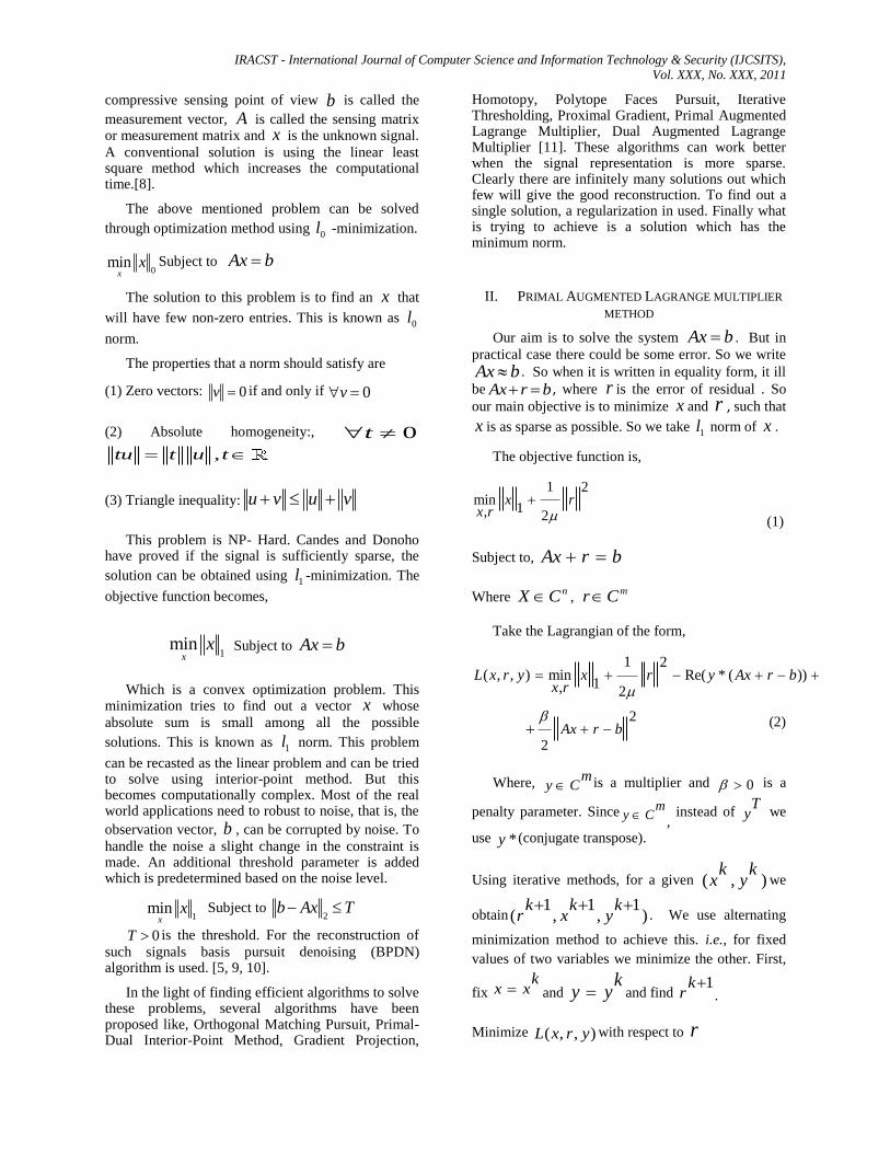
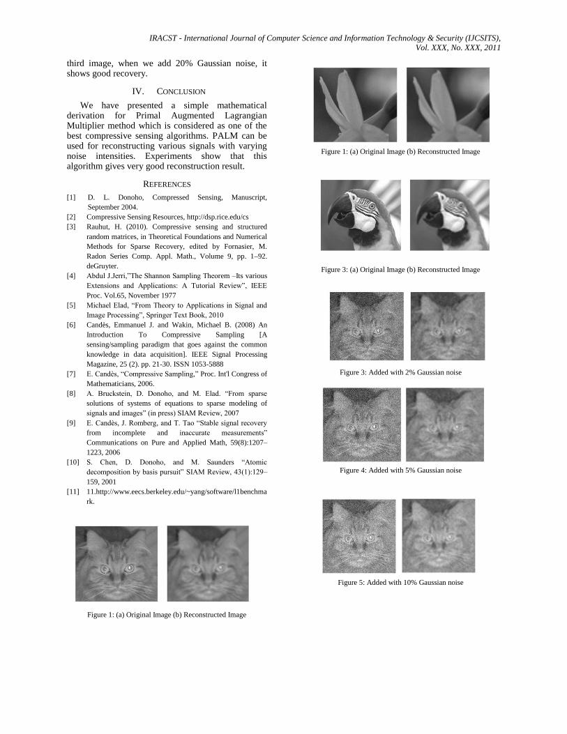
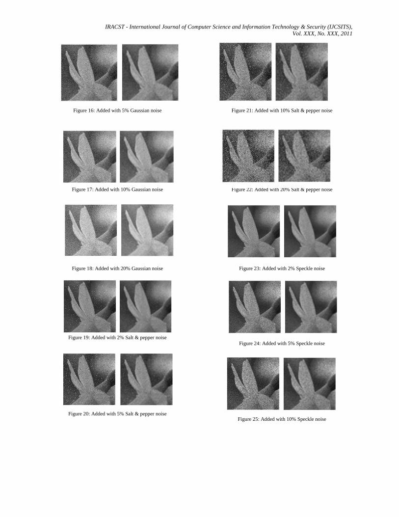
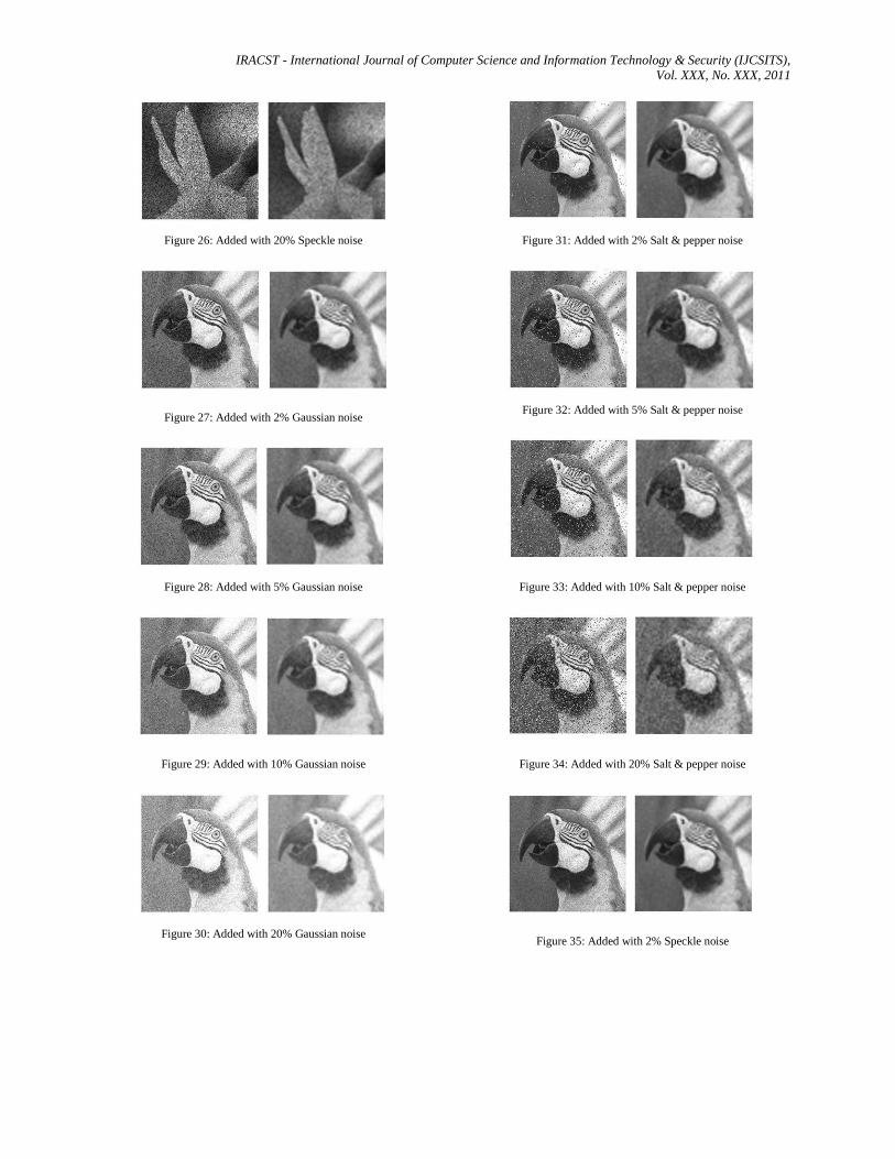
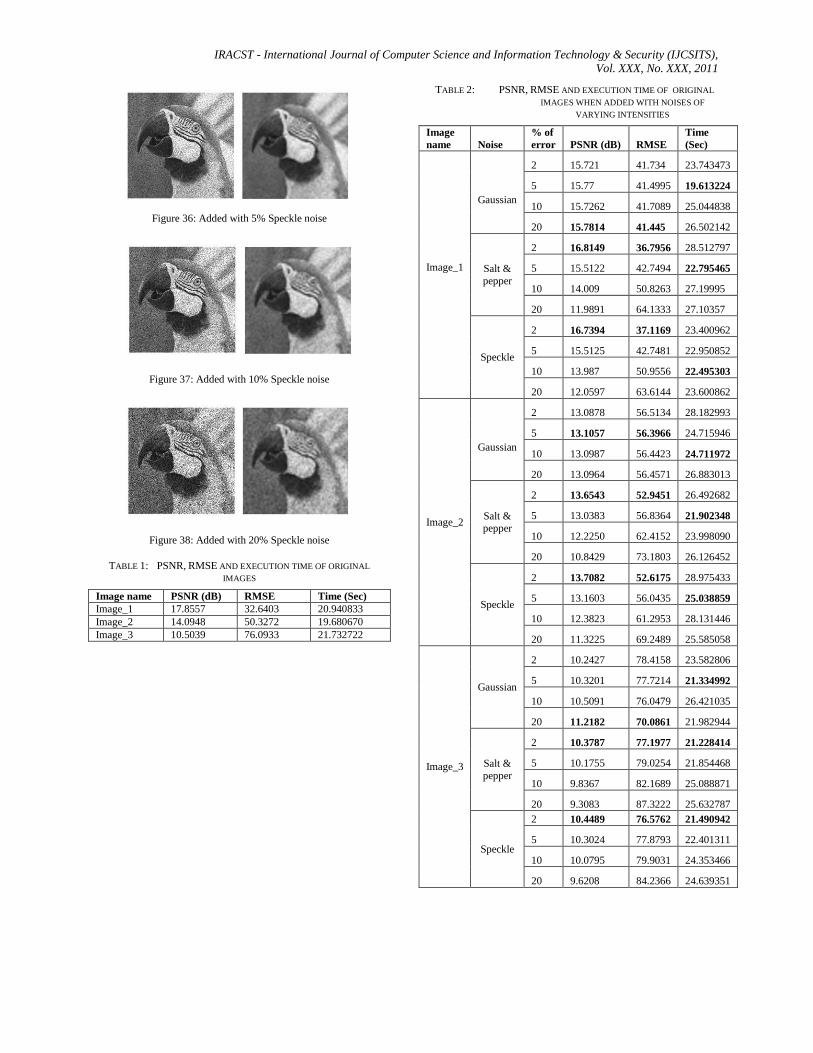
Primal Augmented Lagrangian Multiplier algorithm is tested on three different images of size 256x256 pixels. Then Gaussian, Salt & pepper and Speckle noises with varying percentage of intensities are added onto these images and reconstruct the image using PALM algorithm. PSNR, RMSE and execution time are calculated in each experiment and reported in the tables Table1 and Table2.

In the case of first two images, PSNR is less and RMSE is more for original image. But in the case of



third image, when we add 20% Gaussian noise, it shows good recovery.

IV. CONCLUSION

We have presented a simple mathematical derivation for Primal Augmented Lagrangian Multiplier method which is considered as one of the best compressive sensing algorithms. PALM can be used for reconstructing various signals with varying noise intensities. Experiments show that this algorithm gives very good reconstruction result.

REFERENCES

[1] D. L. Donoho, Compressed Sensing, Manuscript,

September 2004.

[2] Compressive Sensing Resources, http://dsp.rice.edu/cs

[3] Rauhut, H. (2010). Compressive sensing and structured

random matrices, in Theoretical Foundations and Numerical

Methods for Sparse Recovery, edited by Fornasier, M.

Radon Series Comp. Appl. Math., Volume 9, pp. 1–92.

deGruyter.

[4] Abdul J.Jerri,”The Shannon Sampling Theorem –Its various

Extensions and Applications: A Tutorial Review”, IEEE

Proc. Vol.65, November 1977

[5] Michael Elad, “From Theory to Applications in Signal and

Image Processing”, Springer Text Book, 2010

[6] Candès, Emmanuel J. and Wakin, Michael B. (2008) An

Introduction To Compressive Sampling [A

sensing/sampling paradigm that goes against the common

knowledge in data acquisition]. IEEE Signal Processing

Magazine, 25 (2). pp. 21-30. ISSN 1053-5888

[7] E. Candès, “Compressive Sampling,” Proc. Int'l Congress of

Mathematicians, 2006.

[8] A. Bruckstein, D. Donoho, and M. Elad. “From sparse

solutions of systems of equations to sparse modeling of

signals and images” (in press) SIAM Review, 2007

[9] E. Candès, J. Romberg, and T. Tao “Stable signal recovery

from incomplete and inaccurate measurements”

Communications on Pure and Applied Math, 59(8):1207–

1223, 2006

[10] S. Chen, D. Donoho, and M. Saunders “Atomic

decomposition by basis pursuit” SIAM Review, 43(1):129–

159, 2001

[11] 11.http://www.eecs.berkeley.edu/~yang/software/l1benchma

rk.

Figure 1: (a) Original Image (b) Reconstructed Image




Figure 3: Added with 2% Gaussian noise



http://dsp.rice.edu/cs




Figure 7: Added with 2% Salt & pepper noise




Figure 11: Added with 2% Speckle noise










TABLE 1: PSNR, RMSE AND EXECUTION TIME OF ORIGINAL

IMAGES

Image name PSNR (dB) RMSE Time (Sec)

Image_1 17.8557 32.6403 20.940833

Image_2 14.0948 50.3272 19.680670

Image_3 10.5039 76.0933 21.732722

TABLE 2: PSNR, RMSE AND EXECUTION TIME OF ORIGINAL

IMAGES WHEN ADDED WITH NOISES OF

VARYING INTENSITIES

Image

name Noise

% of

error PSNR (dB) RMSE

Time

(Sec)

Image_1

Gaussian

2 15.721 41.734 23.743473

5 15.77 41.4995 19.613224

10 15.7262 41.7089 25.044838

20 15.7814 41.445 26.502142

Salt &

pepper

2 16.8149 36.7956 28.512797

5 15.5122 42.7494 22.795465

10 14.009 50.8263 27.19995

20 11.9891 64.1333 27.10357

Speckle

2 16.7394 37.1169 23.400962

5 15.5125 42.7481 22.950852

10 13.987 50.9556 22.495303

20 12.0597 63.6144 23.600862

Image_2

Gaussian

2 13.0878 56.5134 28.182993

5 13.1057 56.3966 24.715946

10 13.0987 56.4423 24.711972

20 13.0964 56.4571 26.883013

Salt &

pepper

2 13.6543 52.9451 26.492682

5 13.0383 56.8364 21.902348

10 12.2250 62.4152 23.998090

20 10.8429 73.1803 26.126452

Speckle

2 13.7082 52.6175 28.975433

5 13.1603 56.0435 25.038859

10 12.3823 61.2953 28.131446

20 11.3225 69.2489 25.585058

Image_3

Gaussian

2 10.2427 78.4158 23.582806

5 10.3201 77.7214 21.334992

10 10.5091 76.0479 26.421035

20 11.2182 70.0861 21.982944

Salt &

pepper

2 10.3787 77.1977 21.228414

5 10.1755 79.0254 21.854468

10 9.8367 82.1689 25.088871

20 9.3083 87.3222 25.632787

Speckle

2 10.4489 76.5762 21.490942

5 10.3024 77.8793 22.401311

10 10.0795 79.9031 24.353466

20 9.6208 84.2366 24.639351

Insight into Primal Augmented Lagrangian Multilplier Method

Documents

Transcript of Insight into Primal Augmented Lagrangian Multilplier Method