Reliability Enhancements for Real-Time Operations of Electric ...

Reliability Enhancements for Real-Time Operations of Electric Power Systems

by

Xingpeng Li

A Dissertation Presented in Partial Fulfillment

of the Requirements for the Degree

Doctor of Philosophy

Approved November 2017 by the

Graduate Supervisory Committee:

Kory Hedman, Chair

Gerald Heydt

Vijay Vittal

Jiangchao Qin

Arizona State University

December 2017

i

ABSTRACT

The flexibility in power system networks is not fully modeled in existing real-time

contingency analysis (RTCA) and real-time security-constrained economic dispatch

(RT SCED) applications. Thus, corrective transmission switching (CTS) is proposed in

this dissertation to enable RTCA and RT SCED to take advantage of the flexibility in

the transmission system in a practical way.

RTCA is first conducted to identify critical contingencies that may cause viola-

tions. Then, for each critical contingency, CTS is performed to determine the beneficial

switching actions that can reduce post-contingency violations. To reduce computational

burden, fast heuristic algorithms are proposed to generate candidate switching lists. Nu-

merical simulations performed on three large-scale realistic power systems (TVA, ER-

COT, and PJM) demonstrate that CTS can significantly reduce post-contingency vio-

lations. Parallel computing can further reduce the solution time.

RT SCED is to eliminate the actual overloads and potential post-contingency over-

loads identified by RTCA. Procedure-A, which is consistent with existing industry

practices, is proposed to connect RTCA and RT SCED. As CTS can reduce post-con-

tingency violations, higher branch limits, referred to as pseudo limits, may be available

for some contingency-case network constraints. Thus, Procedure-B is proposed to take

advantage of the reliability benefits provided by CTS. With the proposed Procedure-B,

CTS can be modeled in RT SCED implicitly through the proposed pseudo limits for

contingency-case network constraints, which requires no change to existing RT SCED

ii

tools. Numerical simulations demonstrate that the proposed Procedure-A can effec-

tively eliminate the flow violations reported by RTCA and that the proposed Procedure-

B can reduce most of the congestion cost with consideration of CTS.

The system status may be inaccurately estimated due to false data injection (FDI)

cyber-attacks, which may mislead operators to adjust the system improperly and cause

network violations. Thus, a two-stage FDI detection (FDID) approach, along with sev-

eral metrics and an alert system, is proposed in this dissertation to detect FDI attacks.

The first stage is to determine whether the system is under attack and the second stage

would identify the target branch. Numerical simulations demonstrate the effectiveness

of the proposed two-stage FDID approach.

iii

ACKNOWLEDGMENTS

The work presented in this dissertation is sponsored by three projects: 1) “Robust

Adaptive Topology Control” under the Green Electricity Network Integration program

funded by Advanced Research Projects Agency - Energy (ARPA-E) under the United

States (U.S.) Department of Energy (DOE); 2) “Stochastic Optimal Power Flow for

Real-Time Management of Distributed Renewable Generation and Demand Response”

under the Network Optimized Distributed Energy Systems Program funded by ARPA-

E; and 3) “A Verifiable Framework for Cyber-Physical Attacks and Countermeasures

in a Resilient Electric Power Grid” funded by the National Science Foundation, a

United States government agency.

I am very grateful for the instructions and support from my PhD supervisor Dr.

Kory Hedman who is also the chair of my doctoral dissertation defense committee.

During the years working with him, I have gained extensive research experience and

broadened my horizon in the power system area. I am also very grateful to other com-

mittee members: Dr. Gerald Heydt, Dr. Vijay Vittal, and Dr. Jiangchao Qin.

To my friends and fellow researchers, I thank you for all kinds of support you pro-

vide. I would also like to thank my parents for the strong support I have been receiving

for years. Their support paves the road to a promising future for me.

iv

TABLE OF CONTENTS

Page

LIST OF TABLES ........................................................................................................ ix

LIST OF FIGURES ................................................................................................... xiii

NOMENCLATURE .................................................................................................... xvi

CHAPTER

1. INTRODUCTION .................................................................................................. 1

1.1 Background ..................................................................................................... 2

1.2 Motivation ....................................................................................................... 4

1.3 Summary of Contents ...................................................................................... 7

2. LITERATURE REVIEW ...................................................................................... 10

2.1 Power Flow Studies ....................................................................................... 10

2.1.1 AC Power Flow ......................................................................................... 12

2.1.2 DC Power Flow ......................................................................................... 15

2.1.3 Linearized AC Power Flow ....................................................................... 16

2.2 Contingency Analysis .................................................................................... 17

2.2.1 Contingency Types .................................................................................... 19

2.2.2 Procedure ................................................................................................... 21

2.2.3 Contingency List........................................................................................ 22

2.2.4 Results of Contingency Analysis ............................................................... 23

2.2.5 Industry Practices ...................................................................................... 24

2.2.6 Post-contingency Violation Management .................................................. 25

v

CHAPTER Page

2.3 Transmission Switching ................................................................................ 27

2.3.1 TS in Unit Commitment ............................................................................ 28

2.3.2 TS in Optimal Power Flow ........................................................................ 29

2.3.3 TS in Energy Markets ................................................................................ 32

2.3.4 TS in Expansion Planning ......................................................................... 32

2.3.5 TS in Load Shedding Recovery ................................................................. 33

2.3.6 TS in Congestion Management ................................................................. 33

2.3.7 TS with Uncertainty................................................................................... 34

2.3.8 TS as a Corrective Mechanism .................................................................. 35


2.4 Economic Dispatch ....................................................................................... 37

2.4.1 SCED with Renewables............................................................................. 39

2.4.2 Decentralized SCED .................................................................................. 40

2.4.3 SCED with Automatic Generation Control ............................................... 41

2.4.4 SCED with Demand Management ............................................................ 42


2.5 False Data Injection Attacks .......................................................................... 49

2.5.1 FDI Attacks ................................................................................................ 50

2.5.2 FDI Attack Detection ................................................................................. 53

2.6 Parallel Computing ........................................................................................ 56

2.6.1 Motivation of Parallelism .......................................................................... 57

vi

CHAPTER Page

2.6.2 Amdahl’s Law............................................................................................ 58

2.6.3 Parallel Computing in Power Systems ...................................................... 59

3. REAL-TIME CONTINGENCY ANALYSIS ....................................................... 62

3.1 Modeling ....................................................................................................... 63

3.2 Contingency List ........................................................................................... 64

3.3 Critical Contingencies ................................................................................... 65

3.4 Case Studies .................................................................................................. 66

3.5 Parallel Computing ........................................................................................ 68

3.6 Conclusions ................................................................................................... 70

4. REAL-TIME CONTINGENCY ANALYSIS WITH CORRECTIVE

TRANSMISSION SWITCHING................................................................................. 72

4.1 Concept of CTS ............................................................................................. 74

4.2 Metrics ........................................................................................................... 77

4.2.1 Average Violation Reduction ..................................................................... 77

4.2.2 Pareto Improvement .................................................................................. 78

4.2.3 Depth ......................................................................................................... 80

4.3 Algorithms ..................................................................................................... 80

4.3.1 CBCE and CBVE ...................................................................................... 81

4.3.2 RDM .......................................................................................................... 82

4.3.3 EDM .......................................................................................................... 83

4.3.4 Complete Enumeration .............................................................................. 86

vii

CHAPTER Page

4.4 Case Studies .................................................................................................. 86

4.4.1 TVA Cases ................................................................................................. 89

4.4.2 ERCOT Cases ............................................................................................ 98

4.4.3 PJM Cases................................................................................................ 100

4.5 Parallel Computing ...................................................................................... 104

4.6 Conclusions ................................................................................................. 105

5. REAL-TIME SECURITY-CONSTRAINED ECONOMIC DISPATCH WITH

CORRECTIVE TRANSMISSION SWITCHING .................................................... 107

5.1 EMS Procedures .......................................................................................... 109

5.1.1 Procedure-A: SCED with RTCA ............................................................. 110

5.1.2 Procedure-B: SCED with CTS based RTCA ........................................... 115

5.2 SCED Mathematical Formulation ............................................................... 118

5.2.1 Unit Cost Curve ....................................................................................... 119

5.2.2 Objective Function .................................................................................. 122

5.2.3 Constraints ............................................................................................... 122

5.2.4 Models ..................................................................................................... 128

5.2.5 Market Implication .................................................................................. 133

5.3 Case Studies ................................................................................................ 137

5.3.1 Procedure-A: SCED with RTCA ............................................................. 137

5.3.2 Procedure-B: SCED with CTS-based RTCA .......................................... 143

5.4 Conclusions ................................................................................................. 153

viii

CHAPTER Page

6. FALSE DATA INJECTION CYBER-ATTACK DETECTION ......................... 155

6.1 Concept........................................................................................................ 155

6.1.1 State Estimation ....................................................................................... 155

6.1.2 FDI Cyber-Attack .................................................................................... 156

6.2 FDID Metrics .............................................................................................. 159

6.2.1 MLDI ....................................................................................................... 159

6.2.2 BORI ........................................................................................................ 161

6.3 Two-stage FDID Approach ......................................................................... 163

6.3.1 Stage 1: FDI Attack Awareness ............................................................... 163

6.3.2 Stage 2: Target Branch Identification ...................................................... 164

6.4 Case Studies ................................................................................................ 166

6.4.1 FDI Results .............................................................................................. 166

6.4.2 FDID Results ........................................................................................... 170

6.5 Conclusions ................................................................................................. 176

7. CONCLUSIONS................................................................................................. 178

8. FUTURE WORK ................................................................................................ 183

REFERENCES .......................................................................................................... 185

ix

LIST OF TABLES

Table Page

2.1 Comparison between Various ISOs’ RT SCED Applications ............................... 49

3.1 Description of the Practical Systems ..................................................................... 67

3.2 Cumulative Statistics of Contingency Analysis ..................................................... 68

3.3 Average Statistics of Contingency Analysis .......................................................... 68

3.4 Average Solution Time of RTCA with Different Threads .................................... 69

4.1 Branch Loading Levels in the Pre-Contingency, Post-Contingency, and Post-

Switching States for the Example Shown in Fig. 4.3 .................................................. 76

4.2 Examples for Illustrating the Concept of Pareto Improvement for CTS ............... 79

4.3 Cumulative Statistics for the TVA, ERCOT, and PJM Systems ........................... 87

4.4 Average Statistics per Scenario ............................................................................. 87

4.5 Cumulative Statistics per System with 5% Tolerance ........................................... 89

4.6 Cumulative Statistics per System with 10% Tolerance ......................................... 89

4.7 Average Violation Reduction with CTS per System ............................................. 89

4.8 Results of Various CTS Methods on the TVA System.......................................... 90

4.9 Solution Time of RTCA and Various CTS Methods on the TVA System ............ 91

4.10 Results of the 5 Best Switching Actions on the TVA System using CBVE........ 92

4.11 Statistics for Random Variables α and τ .............................................................. 94

4.12 Statistics for Random Variable β ......................................................................... 95

4.13 Statistics for Random Variable φ ......................................................................... 95

4.14 Results of the TVA Cases in the Third Day ........................................................ 97

x

Table Page

4.15 Comparison among a Variety of CTS Methods on the TVA Cases in the Third

Day ............................................................................................................................... 97

4.16 Results of Various CTS Methods on the ERCOT System ................................... 98

4.17 Solution Time of RTCA and Various CTS Methods on the ERCOT System ..... 99

4.18 Results of Various CTS Methods on the PJM System ...................................... 101

4.19 Solution Times of RTCA and Various CTS Methods on the PJM System ....... 101

4.20 Results of the 5 Best Switching Actions on the PJM System using CBVE ...... 101

4.21 Results of Various CTS Methods on the PJM System for the Selected Hours .. 102

4.22 Results of the 5 best CTS Solutions on the PJM System for the Selected Hours

using CBCE ............................................................................................................... 103

4.23 Results of the 5 best CTS Solutions on the PJM System for the Selected Hours

using CBVE ............................................................................................................... 103

4.24 Results of the 5 best Switching Actions on the PJM System for the Selected

Hours using CE .......................................................................................................... 103

4.25 Average CTS Solution Time per System with Different Threads ..................... 104

5.1 Multiple Corrective SCED Models ...................................................................... 130

5.2 Multiple Preventive SCED Models ..................................................................... 132

5.3 Results of RTCA on the Cascadia System ........................................................... 138

5.4 Cost for Different PSCED Models on the Cascadia System ............................... 139

5.5 Computational Time for Solving Different PSCED Models on the Cascadia

System ........................................................................................................................ 140

xi

Table Page

5.6 Results of SCED and Post-SCED N-1 check with Different PSCED Models on

Cascadia ..................................................................................................................... 140

5.7 Results with Different Pct and PctC on the Cascadia System ............................. 142

5.8 SCED Cost with Different Pct and PctC on the Cascadia System ...................... 142

5.9 Computational Time for Solving SCED with Different Pct and PctC on the

Cascadia System ........................................................................................................ 142

5.10 Results of RTCA with CTS on the Cascadia System ........................................ 143

5.11 Emergency Limits of Branch 229 under Contingency 228 with and without CTS

on the Cascadia System ............................................................................................. 145

5.12 Results of Various SCED Models on the Cascadia System .............................. 145

5.13 Results of the Post-SCED RTCA with Different CTS Considered in SCED on

Cascadia ..................................................................................................................... 148

5.14 Results of RTCA with CTS in the Post-SCED Stage with the SCED Solution

Corresponding to the 1st Best CTS Solution Identified in the Pre-SCED Stage on the

Cascadia System ........................................................................................................ 149


Corresponding to the 3rd Best CTS Solution Identified in the Pre-SCED Stage on the

Cascadia System ........................................................................................................ 150


Corresponding to the 4th best CTS Solution Identified in the Pre-SCED Stage on the

Cascadia System ........................................................................................................ 150

xii

Table Page


Corresponding to the 5th Best CTS Solution Identified in the Pre-SCED Stage on the

Cascadia System ........................................................................................................ 150

5.18 Market Results with SCED and Various E-SCED on the Cascadia System ..... 151

5.19 Average LMP with SCED and Various E-SCEDs on the Cascadia System ..... 153

6.1 Alert Level Criteria based on MLDIk or EMLDIk ............................................... 161

6.2 Alert Level Criteria based on BORIk ................................................................... 163

6.3 Alert Level Criteria based on SMLDI................................................................... 164

6.4 Comprehensive Alert Level Combined from Two Separate Alert Levels ........... 165

6.5 SMLDI Values for FDI Malicious Load Deviation Vectors ............................... 172

6.6 SMLDI Values for Random Load Fluctuation Vector ........................................ 172

6.7 Target Line Identification Results for FDI Attacks on Line 111 with a Load Shift

Factor of 10% and No Random Load Fluctuation in the First Dispatch Interval ...... 174

6.8 Target Line Identification Results for FDI Attacks on Line 111 with a Load Shift

Factor of 10% and N(0, 3%) Load Random Fluctuation in the First Dispatch Interval

.................................................................................................................................... 175

6.9 Results of FDID on Various FDI Attacks ............................................................ 176

xiii

LIST OF FIGURES

Figure Page

2.1 Single-Line Diagram of a Two-Terminal Circuit. ................................................. 11

2.2 Single-Line Equivalent Diagram of a Transformer. .............................................. 12

2.3 Contingency Analysis Procedure. .......................................................................... 21

3.1 Illustration of a One-Bus-Island. ............................................................................ 65

3.2 Average Solution Time of RTCA on the ERCOT System. ................................... 70

3.3 Average Parallel Efficiency of RTCA on the PJM System. .................................. 70

4.1 Procedure of Contingency Analysis with Corrective Transmission Switching. .... 73

4.2 An Example of Voltage Violations Fully Eliminated by CTS [141]. .................... 75

4.3 An Example of Flow Violations Fully Eliminated by CTS. .................................. 75

4.4 Flowchart of the Proposed EDM Heuristic. ........................................................... 85

4.5 Violation Reduction with the 5 Best Switching Actions Identified by CBVE on

TVA. ............................................................................................................................ 93

4.6 Cumulative Distribution Function of Random Variable τ. .................................... 95

4.7 Violation Reduction with the 5 Best Switching Actions on the ERCOT System. ....

...................................................................................................................................... 99

4.8 Violation Reduction with the 5 Best Switching Actions on the PJM System. .... 102

4.9 Average CTS Solution Time per Scenario/Hour with Different Threads on the

ERCOT System. ......................................................................................................... 105

5.1 Flowchart of the Proposed Procedure-A for Connecting SCED with RTCA. ..... 111

5.2 Flowchart of the Proposed Procedure-B. ............................................................. 116

xiv

Figure Page

5.3 Block Cost Curve of Generator g......................................................................... 121

5.4 Slope Cost Curve of Generator g. ........................................................................ 121

5.5 Illustration of Linearization of a Slope Segment. ................................................ 121

5.6 System Condition of a Portion of the Cascadia System in the Base Case. .......... 137

5.7 System Condition of a Portion of the Cascadia System under the Outage of

Branch 228. ................................................................................................................ 138

5.8 System Condition of a Portion of the Cascadia System in the Post-Switching

Situation (CTS Branch 37) under the Outage of Branch 228. ................................... 144

5.9 Congestion Costs of the Traditional SCED and Various E-SCEDs on the Cascadia

System. ....................................................................................................................... 146

5.10 Load Payment for Various SCED and E-SCEDs on the Cascadia System. ...... 152

5.11 Congestion Revenue for Various SCED and E-SCEDs on the Cascadia System.

.................................................................................................................................... 152

6.1 Time Line for Illustrating FDI Cyber-Attack ...................................................... 157

6.2 Maximum Power Flow on Line 111 with Various Load Shift Factors and l1-Norm

Constraint Limits. ...................................................................................................... 167

6.3 Maximum Power Flow on Line 118 with Various Load Shift Factors and l1-Norm

Constraint Limits. ...................................................................................................... 167

6.4 Maximum Power Flow on Line 111 with Random Load Fluctuation. ................ 169

6.5 Maximum Power Flow on Line 118 with Random Load Fluctuation. ................ 169

6.6 SMLDI Values for Random Load Fluctuations and FDI Cyber-Attacks. ........... 173

xv

Figure Page

6.7 SMLDI of FDI Attacks for Target Branch 118 with N(0, 3%) Random Load

Fluctuation. ................................................................................................................ 173

xvi

NOMENCLATURE

Abbreviations

ACOPF AC optimal power flow.

AGC Automatic generation control.

ALB Alert level associated with the metric branch overload risk index.

ALC Comprehensive alert level for detecting whether the system is under

cyber-attack.

ALE Alert level associated with the metric enhanced malicious load deviation

index.

ALM Alert level associated with the metric malicious load deviation index.

BORI Branch overload risk index.

CAISO California Independent System Operator.

CBCE Closest branches to contingency element.

CBVE Closest branches to violation element.

CE Complete enumeration.

CI Comprehensive false data injection cyber-attack index.

CPU Central processing unit.

CSCED Corrective security-constrained economic dispatch.

CTS Corrective transmission switching.

DCOPF DC optimal power flow.

DOE Department of Energy.

EDM Enhanced data mining.

xvii

EMLDI Enhanced malicious load deviation index.

EMS Energy management system.

ERCOT Electric Reliability Council of Texas.

E-SCED Enhanced security-constrained economic dispatch.

FDI False data injection.

FDID False data injection detection.

FDPF Fast decoupled power flow.

FERC Federal Energy Regulatory Commission.

ISO Independent System Operator.

IT SCED Intermediate-time security-constrained economic dispatch.

LMP Locational marginal price.

LP Linear programming.

LODF Line outage distribution factors.

MLDI Malicious load deviation index.

NERC North American Electric Reliability Corporation.

MISO Midcontinent Independent System Operator.

NYISO New York Independent System Operator.

ISO-NE Independent System Operator New England.

OPF Optimal power flow.

OTDF Outage transfer distribution factors.

OTS Optimal transmission switching.

PI Pareto improvement

xviii

PJM PJM Interconnection.

PSCED Preventive security-constrained economic dispatch.

PSO Particle swarm optimization.

PTDF Power transfer distribution factors.

QP Quadratic programming.

MIP Mixed integer programming.

MILP Mixed integer linear programming.

RDM Regular data mining.

RTCA Real-time contingency analysis.

RT SCED Real-time security-constrained economic dispatch.

RTD Real-time dispatch.

RTD-CAM Real-time dispatch/corrective auction mode.

RTED Real-time economic dispatch.

RTO Regional Transmission Organization.

RTUC Real-time unit commitment.

SE State estimation.

SCUC Security-constrained unit commitment.

SCED Security-constrained economic dispatch.

SMLDI System-wide malicious load deviation index.

TS Transmission switching.

TVA Tennessee Valley Authority.

xix

Sets

C Critical contingencies.

𝐶𝑠 Critical contingencies under system scenario s.

D Loads.

D(n) Loads that locate at bus n.

D(k) Loads that are critical to branch k.

DN Non-positive loads.

DP Positive loads.

DV Virtual loads.

G Generators.

G(n) Generators that locate at bus n.

GD Generators that are dispatchable.

I Interfaces.

IKM(0) Interfaces lines that are under monitor for base case.

IKM(c) Interfaces lines that are under monitor for contingency case c.

IM(0) Critical interfaces that are under monitor for base case.

IM(c) Critical interfaces that are under monitor for contingency case c.

K Branches.

KA Branches that have the top ten values for malicious load deviation index.

KM(0) Branches that are under monitor for base case.

KI(i) Branches that form the interface i.

K(n-) Branches with bus n as from-bus.

xx

K(n+) Branches with bus n as to-bus.

KM(c) Branches that are under monitor for contingency c.

N Buses.

Parameters

𝑏𝑚𝑛 Susceptance of the branch connecting bus m to bus n.

𝑏𝑚𝑛0 Total charging susceptance of a transmission connecting bus m to bus n.

𝑏𝑚𝑛0,𝑚 Magnetizing susceptance at the terminal m of the transformer connect-

ing bus m to bus n.

𝑏𝑚𝑛0,𝑛 Magnetizing susceptance at the terminal n of the transformer connecting

bus m to bus n.

𝐵𝑆𝑔,𝑖 Breadth of segment i for unit g.

𝐶𝑔,𝑖 Cost for segment i of unit g.

𝐶𝑆𝑅𝑔 Spinning reserve price for unit g.

𝑔𝑚𝑛 Conductance of the branch connecting bus m to bus n.

𝐿𝐿𝑘0 Initial loading level of branch k in the base case.

𝐿𝐿𝑘𝑐0 Initial loading level of branch k under contingency c.

𝐿𝑖𝑚𝑖𝑡𝐴𝑘 Normal thermal limit in MW for branch k in SCED.

𝐿𝑖𝑚𝑖𝑡𝐶𝑘𝑐 Emergency thermal limit in MW for branch k under contingency c in

SCED.

𝐿𝑖𝑚𝑖𝑡𝑖 Total flow limit in MW for interface i in SCED.

𝐿𝑖𝑚𝑖𝑡𝑖𝑐 Total flow limit in MW for interface i under contingency c in SCED.

𝐿𝑂𝐷𝐹𝑘,𝑐 Line c outage distribution factor on line k.

xxi

𝑀𝑅𝑅𝑔 Energy ramp rate (MW/minute or p.u./minute) for unit g.

𝑛(𝑑) Bus where load d locates.

𝑛(𝑘−) From-bus of branch k.

𝑛(𝑘+) To-bus of branch k.

𝑁1 The limit of an 𝑙1-norm constraint.

𝑁𝐷𝑘 Number of loads that are critical to branch k.

𝑁𝑆𝑔 Number of cost segments for unit g.

𝑛𝑆𝑆 The number of sub-segments for a slope segment of unit slope cost

curve.

𝑂𝑇𝐷𝐹𝑛,𝑘,𝑐 Outage transfer distribution factor from bus n to line k when line c is

outage.

𝑃𝑐𝑡 Threshold (a percent number) for determining base-case monitor set.

𝑃𝑐𝑡𝐶 Threshold (a percent number) for determining contingency-case monitor

set.

𝑃𝑐0 Active power of the contingency generator c in the pre-contingency sit-

uation.

𝑃𝑑 Target/forecasting active power of load d at the end of a SCED period.

𝑃𝑑0 Initial active power of load d at 𝑡 = 0 or at the beginning of a SCED

period.

𝑃𝑑0,𝐼𝑆𝑂 Measurement of load d at 𝑡 = 0.

𝑃𝑑− Actual load d at 𝑡 = −𝑇𝐸𝐷.

𝑃𝐹_𝑃𝐷𝑠ℎ𝑒𝑑 A fix penalty factor for variable 𝑝𝑑,𝑠ℎ𝑒𝑑 and 𝑝𝑑,𝑠ℎ𝑒𝑑,𝑐.

xxii

𝑃𝑔0 Active power of unit g in the pre-contingency situation.

𝑃𝑔0 Initial output of unit g.

𝑃𝑔,𝑚𝑎𝑥 Maximum output for unit g.

𝑃𝑔,𝑚𝑖𝑛 Minimum output for unit g.

𝑃𝑘0 Initial active flow on branch k flowing out of from-bus in SCED.

𝑃𝑘0,𝑓𝑟𝑜𝑚 Initial active power on branch k flowing out of the from-bus.

𝑃𝑘0,𝐼𝑆𝑂 Measurement of active flow on branch k at 𝑡 = 0.

𝑃𝑘0,𝑡𝑜 Initial active power on branch k flowing out of the to-bus.

𝑃𝑘,𝑐,0 Initial active flow on branch k under contingency c flowing out of from-

bus in SCED.

𝑃𝑘𝑐0,𝑓𝑟𝑜𝑚 Initial active power on branch k flowing out of from-bus under contin-

gency c.

𝑃𝑘𝑐0,𝑡𝑜 Initial active power on branch k flowing out of the to-bus under contin-

gency c.

𝑃𝑘− Actual active flow on branch k at 𝑡 = −𝑇𝐸𝐷.

𝑃𝑘+,𝑆𝐶𝐸𝐷 Active flow on branch k at 𝑡 = 𝑇𝐸𝐷, determined by SCED that runs at

𝑡 = 0.

𝑃𝑇𝐷𝐹𝑛,𝑘 Power transfer distribution factor from bus n to line k.

𝑃𝑇𝐷𝐹𝑛(𝑑),𝑘 Power transfer distribution factor from load d to line k.

𝑄𝑘0,𝑓𝑟𝑜𝑚 Initial reactive power on branch k flowing out of the from-bus.

𝑄𝑘0,𝑡𝑜 Initial reactive power on branch k flowing out of the to-bus.

xxiii

𝑄𝑘𝑐0,𝑓𝑟𝑜𝑚 Initial reactive power on branch k flowing out of from-bus under con-

tingency c.

𝑄𝑘𝑐0,𝑡𝑜 Initial reactive power on branch k flowing out of the to-bus under con-

tingency c.

𝑅𝑎𝑡𝑒𝐴𝑘 Normal thermal limit in MVA for branch k in power flow calculations.

𝑅𝑎𝑡𝑒𝐶𝑘 Emergency thermal limit in MVA for branch k in power flow calcula-

tions.

𝑟𝑚𝑛 Resistance of the branch connecting bus m to bus n.

𝑠𝑖𝑔𝑛(𝑃𝑘0) 1 if actual flow direction is from from-bus to to-bus; -1 if actual flow

direction is from to-bus to from-bus.

𝑆𝑘0,𝑓𝑟𝑜𝑚 Initial complex power on branch k flowing out of the from-bus.

𝑆𝑘0,𝑡𝑜 Initial complex power on branch k flowing out of the to-bus.

𝑆𝑘𝑐0,𝑓𝑟𝑜𝑚 Initial complex power on branch k flowing out of from-bus under con-

tingency c.

𝑆𝑘𝑐0,𝑡𝑜 Initial complex power on branch k flowing out of the to-bus under con-

tingency c.

𝑆𝑅𝑎 Spinning reserve requirement for area a.

𝑆𝑅𝑅𝑔 Spinning ramp rate (MW/minute or p.u./minute) for unit g.

𝑡𝑚 Transformer tap ratio at terminal m.

𝑇𝐸𝐷 Look-ahead time for SCED, or the time length of a SCED period.

𝑇𝑆𝑅 Time for spinning reserve requirements.

𝑉𝑚𝑎𝑥 Maximum limit of voltage magnitude.

xxiv

𝑉𝑚𝑖𝑛 Minimum limit of voltage magnitude.

𝑋𝑘 Reactance of branch k.

𝑥𝑚𝑛 Reactance of the branch connecting bus m to bus n.

𝑦𝑚𝑛 Admittance of the branch connecting bus m to bus n.

𝑧𝑚𝑛 Impedance of the branch connecting bus m to bus n.

𝑣𝑘𝑐 The violation on branch k under contingency c.

𝑣𝑘𝑐,𝐶𝑇𝑆 The violation on branch k under contingency c with corrective transmis-

sion switching action implemented.

𝛼𝑘 Phase angle of branch k; 0 if the branch is not a phase shifter.

∆𝑏𝑖 The initially selected breadth of a sub-segment for a slope segment of

unit slope cost curve.

∆𝑠 The actual breadth of each sub-segment for a slope segment of unit slope

cost curve.

Variables

𝐴𝑣𝑔𝐿𝑀𝑃 Average locational marginal price over all buses in the system.

𝐴𝑣𝑔𝐿𝑀𝑃𝑐𝑔 Average of congestion component of locational marginal price over all

buses in the system.

𝐶𝐶𝑅𝐶𝑇𝑆 Congestion cost reduction.

𝑐𝑛 Change in phase angle at bus n due to attack.

𝐶𝑛𝑔𝑠𝑡𝐶𝑜𝑠𝑡 Total congestion cost over the entire system.

𝐶𝑛𝑔𝑠𝑡𝑅𝑣𝑛 Total congestion revenue over the entire system.

𝐷𝐶𝑇𝑆 Average depth of switching solutions.

xxv

𝐸𝑀𝐿𝐷𝐼𝑘 The enhanced malicious load deviation index of branch k.

𝐸𝑝 Parallel efficiency (a percent number).

𝐹𝑔𝑐 Participation factor of unit g under a generator contingency c.

𝐹𝜏 Cumulative distribution function of variable 𝜏.

𝐺𝑒𝑛𝐶𝑜𝑠𝑡 Total generator cost over the entire system.

𝐺𝑒𝑛𝑅𝑒𝑛𝑡 Total generator rent over the entire system.

𝐼𝑓𝑑,𝑘 Influential factor for branch k due to the change in load d.

𝐼𝑛𝑑𝑖𝑐𝑡𝑟𝑑,𝑘 1 if significant change in load d decreases the absolute flow on branch

k; 0 if the change in load d is trivial; -1 if significant change in load d

increase the absolute flow on branch k.

𝐿𝐶𝑇𝑆,𝑐 The location of the switching solution in the candidate list for contin-

gency c.

𝐿𝑑𝑃𝑎𝑦𝑚𝑡 Total load payment over the entire system.

𝐿𝑀𝑃𝑐𝑔,𝑛 Congestion component of locational marginal price at bus n.

𝐿𝑀𝑃𝑛 Locational marginal price at bus n.

𝐿𝑀𝑃𝑠 System-wide locational marginal price.

𝐿𝑆 Load shift factor.

𝐺𝑒𝑛𝑅𝑣𝑛 Total generator revenue over the entire system.

𝑁𝑐 Total number of critical contingency.

𝑀𝐿𝐷𝐼𝑘 The malicious load deviation index of branch k.

𝑀𝑐 Total number of critical contingencies for which at least a beneficial

switching solution exists.

xxvi

𝑝𝑑,𝑠ℎ𝑒𝑑 Shedded active power for load d.

𝑝𝑑,𝑠ℎ𝑒𝑑,𝑐 Shedded active power for load d under contingency c.

𝑝𝑔 Total output of generator g.

𝑃𝑔𝑐 Active power output of unit g under generator contingency c for gener-

ator contingency analysis.

𝑝𝑔,𝑐 Total output of generator g under contingency c for SCED.

𝑝𝑔,𝑖 Output on segment i for generator g.

𝑃𝐼𝑛 Active power injection at bus n.

𝑝𝑖 Total flow for interface i.

𝑝𝑖,𝑐 Total flow for interface i under contingency c.

𝑝𝑘 Power flow on branch k.

𝑝𝑘 Cyber flow on branch k.

𝑝𝑘,𝑐 Flow on branch k under contingency c.

𝑃𝑚𝑛 Active power flowing from bus m to bus n.

𝑃𝑛𝑚 Active power flowing from bus n to bus m.

𝑄𝑚𝑛 Reactive power flowing from bus m to bus n.

𝑄𝑛𝑚 Reactive power flowing from bus n to bus m.

𝑆𝑛 Speedup achieved with parallel computing.

𝑆𝑝,𝑚𝑎𝑥 Maximum possible speedup achieved with parallel computing.

𝑠𝑟𝑔 Spinning reserve that generator g provides.

𝑇𝑛 Computational time of parallel computing with n threads.

𝑇𝑠 Computational time of the sequential program.

xxvii

𝑣𝑐0 Total violations in the post-contingency situation.

𝑣𝑐1 Total violations in the post-switching situation for contingency c.

𝑉𝑚 Voltage magnitude at bus m.

𝑉𝑛 Voltage magnitude at bus n.

𝜃𝑚𝑛 Phase angle difference across the transmission connecting bus m and bus

n.

𝜃𝑚𝑛,𝑠 Phase angle setting of the phase shifting transformer connecting bus m

and bus n.

𝜃𝑛 Actual phase angle at bus n.

�̃�𝑛 Cyber phase angle at bus n.

𝜃𝑠 Phase angle difference of the phase shifter transformer connecting bus

m to bus n.

𝛿𝑛(𝑘−) Phase angle of bus 𝑛(𝑘−).

𝛿𝑛(𝑘−),𝑐 Phase angle of bus 𝑛(𝑘−) under contingency c.

𝛿𝑛(𝑘+) Phase angle of bus 𝑛(𝑘+).

𝛿𝑛(𝑘+),𝑐 Phase angle of bus 𝑛(𝑘+) under contingency c.

𝜂𝐶𝑇𝑆 Average violation reduction in percent.

𝑤𝑐 Probably of contingency c.

𝛼 The number of scenarios for which the same contingency is identified

as a critical contingency, used for analyzing the enhanced data mining

method.

xxviii

𝜏 The probability of a contingency being identified as a critical contin-

gency, used for analyzing the enhanced data mining method.

𝛾 The number of scenarios where at least a beneficial CTS solution exists

for a critical contingency, used for analyzing the enhanced data mining

method.

𝛽 The probability that at least a beneficial CTS solution exists for an iden-

tified critical contingency, used for analyzing the enhanced data mining

method.

𝜑 The number of switching actions in the candidate list, obtained from the

enhanced data mining method, for a critical contingency.

∆𝑝𝑑 The malicious deviation of load d.

∆𝑝𝑘 The difference between the post-attack actual and cyber power flows on

branch k.

1

1. INTRODUCTION

A power system is an electrical network of interconnected elements that are used

to generate, transmit, and consume electric power. It consists of, but not limited to,

generators, loads, transmission lines, transformers, phase shifters, circuit breakers, and

shunts. High voltage direct current lines may exist in some power systems.

The prime function of an electrical network is to transmit and distribute power. The

voltage level varies from several hundred volts to around one thousand kilovolts (kV).

A power system network can be divided into two portions: a high-voltage level trans-

mission subsystem and a low-voltage level distribution subsystem.

The asset value of infrastructure in the North American power system represents

more than 1 trillion United States (U.S.) dollars. The electricity grid of the United States

contains over 360,000 miles of transmission lines including around 180,000 miles of

high-voltage lines and connects to over 6,000 power plants in 2012 [1]. Reference [1]

also reports that: 1) in 2011, the global power generation capacity, which grows by 2%

annually, is about five trillion watts; 2) the two countries that have the largest genera-

tion capacity are the United States and China, each of which accounts for approximately

20% of the world’s total installed capacity; 3) the generation capacity in China will

increase by about 3% per year through 2035 while the capacity growth in the United

States is less than 1% during the same period.

Only 10% of the energy consumption in America was used to produce electricity

in 1940; this percentage increased to 25% in 1970 and it was around 40% in 2003 [2].

This implies the efficiency of electricity as a source for supplying energy is increasing.

2

As introduced in [3], 56% of the electricity generated in the United States in 2012 was

provided by coal-fired power plants and nuclear power plants.

There are more than 3,100 electric companies, utilities, and regulation organiza-

tions in the United States. For instance, Federal Energy Regulatory Commission

(FERC) regulates interstate transmission networks and energy markets [4]; North

American Electric Reliability Corporation (NERC) ensures the reliability of the power

systems in North America by developing reliability standards [5].

Independent System Operators (ISOs) were created under FERC Order 888 and

Order 889. The goal of the ISOs is to meet the requirements of providing unbiased open

access to transmission. Subsequently, FERC issued Order 2000 that presents the re-

quirements to be a Regional Transmission Organization (RTO). Voluntary formation

of RTO was encouraged by FERC to manage the regional transmission network [6].

The ISOs/RTOs in the United States include California ISO (CAISO), New York ISO

(NYISO), ISO New England (ISO-NE), Midcontinent ISO (MISO), PJM Interconnec-

tion (PJM), Southwest Power Pool, and Electric Reliability Council of Texas (ERCOT).

Note that ERCOT is governed by the Public Utility Commission of Texas rather than

FERC.

1.1 Background

As energy cannot be economically stored on a large scale, electricity must be pro-

duced, transported, and consumed at the same time. Therefore, it is very challenging to

maintain reliable real-time operations of power systems. Failure of any element may

3

have a negative effect on the normal operations of power systems. Hence, it is essential

to improve power system security and reliability.

Power systems are built with some degree of redundancy due to concerns regarding

power system security. In addition, a number of mandatory standards for power system

reliability have been developed recently. Complying with these standards makes the

system less susceptible. However, power systems are complex and dynamical in nature,

which makes it hard to operate them properly. Uncertainty such as load fluctuation

makes it more difficult to maintain power system security in real-time. Thus, power

system real-time secure operations have gained increased attention. Operators are

forced to make preventive adjustments in advance or take just-in-time corrective actions

in order to maintain power system security in the event of a disturbance.

System security consists of three major functions [7], which includes:

• System monitoring,

• Contingency analysis,

• Security-constrained economic dispatch (SCED).

These are key functions of energy management systems (EMSs) used in modern power

systems. The system monitoring function determines the system condition and provides

a base for contingency analysis and security-constrained economic dispatch. Contin-

gency analysis identifies potential post-contingency violations, which will be corrected

by SCED.

The system monitoring function receives data from remote terminal units or local

control centers and then performs state estimation (SE) to determine the real-time status

4

of the system, including bus voltage magnitude and angle. Thus, with this function,

system operators will be informed immediately when branch overloads and voltage

limit violations occur. It provides system operators with the actual real-time system

condition, as well as a base case for other real-time applications.

Contingency analysis evaluates the impact of a potential contingency on system

security. Contingency analysis when simulated in real-time is referred to as real-time

contingency analysis (RTCA). With the results obtained from RTCA, the system can

operate defensively in real-time. A contingency may cause serious consequences in a

short time and operators may not have sufficient time to react to the contingency, pre-

vent the situation from getting worse, and restore the system. Thus, the goal of RTCA

is to enable system operators to be better prepared with pre-planned strategies to deal

with potential critical contingencies.

SCED aims to provide a least-cost re-dispatch solution for online units while meet-

ing the network constraints as well as other restrictions. When simulated in real-time,

SCED is referred to as real-time SCED (RT SCED). Actual network violations obtained

from state estimation or base-case power flow and potential post-contingency network

violations obtained from RTCA will be sent to RT SCED as network constraints and

are supposed to be eliminated with the new dispatch point obtained from RT SCED in

the post-SCED steady state.

1.2 Motivation

Power system operations need to satisfy physical constraints such as Kirchhoff's

laws and comply with reliability standards. Improper real-time operations may result in

5

system violations, islanding, irreversible damage to electrical equipment, and in the

worst-case a blackout. Therefore, improving system reliability in real-time operations

is very important. This dissertation focuses on reliability enhancements for real-time

operations of electric power systems.

The ISOs typically use energy management systems to help system operators mon-

itor and manage the system in real-time. Key functions of the EMS include system

monitoring, RTCA, and RT SCED. System monitoring observes the system condition

and provides a base case for all other real-time applications. RTCA identifies critical

contingencies and the associated violations and forms network constraints for RT

SCED. RT SCED produces a generation re-dispatch solution that would eliminate the

actual base-case network constraints and the potential contingency-case network viola-

tions identified by RTCA and meet all the system requirements at least cost.

Electrical networks are built with some level of redundancy due to security con-

cerns. They are traditionally considered as static assets in power system real-time op-

erations. However, the flexibility in electrical network has not been fully utilized and

reflected in existing operational tools. Prior research efforts have illustrated that trans-

mission switching (TS) can provide a variety of benefits for power system operations.

Transmission switching is a control strategy that switches a branch out of service to

achieve a particular goal.

Though transmission switching has not been widely used as a regular strategy in

reality, it is being used as an emergency corrective control scheme for some parties,

6

which is referred to as corrective TS (CTS). The switching actions are mainly deter-

mined based on ad-hoc methods and it is unclear how CTS would improve and fit in

existing operational applications. In this dissertation, the reliability enhancements pro-

vided by CTS are investigated and a systematic procedure is proposed in order to inte-

grate CTS into RTCA and RT SCED. The proposed integrating procedure will require

minimal change to existing operational tools.

Given a base case, provided by the system monitoring function of EMS, RTCA

will first execute and identify critical contingencies that are to be sent to the CTS rou-

tine. Several heuristic approaches are proposed to generate a ranked candidate switch-

ing list. Five beneficial switching actions, which would reduce or eliminate the post-

contingency violations, are identified for each of those critical contingencies. Numeri-

cal simulations on three large-scale practical systems demonstrate the effectiveness of

CTS. Simulation results also show that parallel computing can speed up the entire pro-

cess including both contingency analysis routine and transmission switching routine.

Modeling CTS in RT SCED directly will largely increase the computational time,

which makes it impossible for real-time applications. In this dissertation, a practical

heuristic is proposed to capture the benefits provided by CTS in RT SCED, as a result

of which existing RT SCED model can remain the same. With the proposed heuristic,

the branch limits of the network constraints that are sent from RTCA to RT SCED

would increase, which can then reduce congestion cost significantly and enable RT

SCED to obtain a solution with a lower total cost. The increased limit is referred to as

a pseudo limit; and a SCED with pseudo limits is referred to as an enhanced SCED (E-

7

SCED) in this dissertation. Simulation results demonstrate that the proposed E-SCED

approach can reduce congestion cost significantly and the CTS actions identified for a

critical contingency in the pre-SCED situation can still reduce the violations under the

same contingency in the post-SCED situation.

As stated above, state estimation estimates the system condition and provides a

starting point for RTCA and RT SCED. Thus, it is very important to ensure the correct-

ness of state estimation. Bad data detection and identification can filter out large ran-

dom measurement errors. However, malicious false data injection (FDI) cyber-attacks

can bypass traditional bad data detection and cause branch overloads that are not ob-

served by system operators. Thus, it is vital to develop a strategy that can effectively

detect FDI attacks in real-time. Several metrics that monitor abnormal load deviations

and flow changes are proposed in this dissertation. Qualitative analysis can be con-

ducted with the proposed FDI cyber-attack alert system. A systematic two-stage FDID

approach is proposed to determine whether the system is under attack and identify the

target branch. Case studies validate the proposed metrics, alert system, and systematic

two-stage FDID approach.

1.3 Summary of Contents

The rest of this dissertation is structured as follows. A thorough literature review

is presented in Chapter 2. In this chapter, power flow studies are first presented, fol-

lowed by a comprehensive introduction of contingency analysis. Then, a systematic

review of past transmission switching research is presented, as well as a detailed review

on economic dispatch and false data injection cyber-attack and detection. At the end of

8

this chapter, an overview of general parallel computing technology and its various ap-

plications in the power system area are presented.

Chapter 3 focuses on RTCA only. The RTCA model used in this dissertation is

first introduced, followed by a discussion on the contingency list as well as the defini-

tion of critical contingencies. Case studies show that three large-scale practical systems

are vulnerable to several contingencies. Parallel computing is also conducted to speed

up the contingency analysis process.

In Chapter 4, the fundamentals of how transmission switching benefits the system

are introduced and the metrics for defining a beneficial switching action are proposed.

Heuristic algorithms are proposed to generate a list of candidate switching branches.

Numerical simulations are then presented to demonstrate the effectiveness of CTS. It is

shown that CTS is a promising strategy in industry. Parallel computing enhances this

viewpoint by further reducing the solution time.

Chapter 5 first presents how the network constraints are obtained from RTCA and

then introduces a typical RT SCED model used in industry. The procedure of consid-

ering CTS in RT SCED is described in detail. Multiple RT SCED models with different

forms of network constraints are simulated and compared. With the most precise SCED

model, the effects of CTS on SCED results are investigated. The benefits of CTS are

also validated by running RTCA with a different base case representing the post-SCED

situation. Case studies show that the congestion cost can be reduced significantly with

CTS.

9

Chapter 6 studies cyber-physical system security. The effects of FDI attacks on

power systems are examined and it is shown that FDI can result in physical flow viola-

tions. Several metrics are proposed in this chapter, as well as an FDI cyber-attack alert

system. The proposed metrics can monitor malicious load deviations as well as suspi-

cious flow changes. A systematic two-stage FDID approach is proposed to detect po-

tential FDI attacks. Cases studies demonstrate the effectiveness of the proposed two-

stage FDID approach.

Chapter 7 concludes this dissertation and potential future work is presented in

Chapter 8.

10

2. LITERATURE REVIEW

2.1 Power Flow Studies

In power system engineering, a power flow study is the basis for steady-state anal-

ysis of the interconnected system. There are transmission system power flow studies

and distribution system power flow studies. This dissertation only focuses on transmis-

sion system power flow studies. Thus, the system can be assumed to be three-phase

balanced and only positive sequence network is modeled. Single-line diagrams and the

per unit system are used to simply the analysis. The pi-equivalent circuit model is typ-

ically used to represent branches. Then, a power flow problem can be solved through

computer programs under those assumptions and the information listed below will be

reported:

• voltage magnitude and phase angle at each bus,

• active power injection and reactive power injection at each bus,

• active power flows and reactive power flows on each branch.

Two widely used models are the full AC power flow model and the simplified DC

power flow model, which will be presented below. The power flow models are used for

solving most problems in the power system domain. Hence, power flow studies are

remarkably important for various power system applications including RTCA, RT

SCED, and the proposed CTS. Note that RTCA and CTS implemented in this disserta-

tion use the AC power flow model while RT SCED uses the DC power flow model.

AC feasibility of the solutions obtained from RT SCED is verified through AC power

flow simulations.

11

Fig. 2.1 shows the single-line diagram of a typical two-terminal circuit, which is

an essential component of a transmission network. Note that P and Q denote active

power and reactive power respectively. The power flowing out of one terminal does not

equal to the power flowing into the other terminal because of the losses on the branch

connecting those two buses, which means that 𝑃𝑚𝑛 ≠ −𝑃𝑛𝑚 and 𝑄𝑚𝑛 ≠ −𝑄𝑛𝑚. The

branch power flow equations are shown below,

𝑃𝑚𝑛 = 𝑉𝑚2𝑔𝑚𝑛 − 𝑉𝑚𝑉𝑛(𝑔𝑚𝑛 cos 𝜃𝑚𝑛 + 𝑏𝑚𝑛 sin 𝜃𝑚𝑛) (2.1)

𝑄𝑚𝑛 = −𝑉𝑚2 (𝑏𝑚𝑛 +

𝑏𝑚𝑛0

2) + 𝑉𝑚𝑉𝑛(𝑏𝑚𝑛 cos 𝜃𝑚𝑛 − 𝑔𝑚𝑛 sin 𝜃𝑚𝑛) (2.2)

where,

𝑦𝑚𝑛 = 𝑔𝑚𝑛 + 𝑗𝑏𝑚𝑛 =1

𝑧𝑚𝑛=

𝑟𝑚𝑛−𝑗𝑥𝑚𝑛

𝑟𝑚𝑛2 +𝑥𝑚𝑛

2 (2.3)

i

0b

2

mnj

j

mn mn mnz = r + jx

Pmn+jQmn1 Pnm+jQnmPmn+jQmn Pnm+jQnm1

Qmn0 Qnm0

0b

2

mnj

Fig. 2.1 Single-Line Diagram of a Two-Terminal Circuit.

Fig. 2.2 shows a single-line equivalent diagram of a transformer. A transformer is

typically represented by a pi-equivalent circuit and an ideal transformer. The tap ratio

is tm for bus m and is one for the nominal end n. 𝑏𝑚𝑛0,𝑚 and 𝑏𝑚𝑛0,𝑛 are the magnetizing

susceptances. In this dissertation, they are set equal for simplification. The power flow

equations for transformers can be derived by replacing 𝑉𝑚 with 𝑉𝑚/𝑡𝑚 and replacing

12

𝑏𝑚𝑛0/2 with 𝑏𝑚𝑛0,𝑚 in the transmission power flow equations (2.1) and (2.2). For a

phase shifting transformer, an extra modification is to replace 𝜃𝑚𝑛 with 𝜃𝑚𝑛 − 𝜃𝑚𝑛,𝑠,

where 𝜃𝑚𝑛,𝑠 is the phase angle setting of this phase shifting transformer.

m

0,mmnb

n

mn mn mny g jb

0,mn nb

:1mt

mn mnP jQnm nmP jQ

1mn mnP jQ 1nm nmP jQ

0mnQ0nmQ

Fig. 2.2 Single-Line Equivalent Diagram of a Transformer.

2.1.1 AC Power Flow

A number of different AC power flow algorithms have been developed in the lit-

erature [8]-[9]. Several well-known iterative approaches include Gauss-Seidel method,

Newton-Raphson method, and fast decoupled power flow (FDPF) method. There are

three basic types of buses: PV buses, PQ buses, and slack buses.

A PV bus is a bus that has the capability of controlling its voltage magnitude and

it is usually a generator bus or a bus whose voltage magnitude is controlled by nearby

generators or other devices such as switched shunts and static VAR compensator. A PQ

bus is typically a load bus or a connection bus. A slack bus should be a bus where there

is a large amount of generation capacity. For some power flow algorithms including the

Newton-Raphson method, a normal assumption is that the slack bus is used to balance

13

the generation and demand. A slack bus is also referred to as the swing bus, angle ref-

erence bus, or just 𝑉𝜃 bus.

In a power flow study, the voltage magnitude and voltage angle at a slack bus are

fixed; the active power and voltage magnitude at PV buses remain the same; and the

active power and reactive power at PQ buses are fixed. The generator reactive power

output Q will adjust automatically to maintain the voltage set point. In reality, the reac-

tive power output Q has its minimum limit and maximum limit. Therefore, a PV bus

may have to switch to a PQ bus when the Q at that bus reaches its limit. Another strategy

for not violating generators’ reactive power limits is to adjust the voltage set values at

the PV buses when the associated reactive power capacity constraints are violated [8].

Gauss-Seidel Method

The Gauss-Seidel approach was the first method to solve the power flow problem

on digital computers [8]. Although each iteration of this approach is fast, it is slow

overall since it typically takes many iterations before it converges with the desired ac-

curacy. It may fail to converge when the system contains negative reactance branches

(compensated transmission lines). The determination of the initial point is critical for

the algorithm convergence.

Newton-Raphson Method

The robust and reliable Newton-Raphson approach is widely used in practice for

solving the power flow problem. The key of this approach is to create the Jacobian

matrix based on the nodal power mismatch functions; then a set of linear equations are

solved simultaneously to obtain an updated solution. This process repeats itself until

14

the specified stopping criteria are satisfied or the maximum number of iterations is

reached. State variables have to be updated between each iteration, as well as the Jaco-

bian matrix. The converged solution may be different with different starting points.

Fast Decoupled Power Flow

The fast decoupled power flow algorithm is developed based on the Newton-

Raphson method. The Newton-Raphson method is robust but it may be slow as the

Jacobian matrix has to be updated per iteration, which accounts for a significant percent

of the total computational time.

Considering the fact that transmission branches typically have high reactance-to-

resistance (X/R) ratios, the Newton-Raphson method can be simplified to accelerate

convergence. One popular simplified method is the fast decoupled power flow method,

which was originally proposed in [9] in 1974. Therefore, another term for FDPF is the

Stott decoupled power flow method, named after the first author of [9]. After FDPF

was first proposed, it has been further enhanced to make the algorithm more robust.

The assumptions of standard FDPF method include that 1) the interaction between

active power and voltage magnitude is neglected, 2) the interaction between reactive

power and voltage angle is neglected, and 3) the angle difference across a branch is

small enough such that the associated cosine value can be assumed to be one. Assump-

tions 1) and 2) are based on engineering experience and observations: the voltage mag-

nitude would not be significantly affected by the active power and the voltage angle

will not change much due to change in reactive power.

15

The power flow converges when both the active power unbalance and the reactive

power unbalance of each bus are less than the predefined tolerances. Though the toler-

ances for active power convergence and reactive power convergence are usually set to

the same values, they do not have to be identical.

The above standard FDPF method is called the XB method. Another similar

method is known as the BX method. The BX method may have a better convergence

performance than the XB method when the system contains transmission lines with low

X/R ratio [10]. The Jacobian matrix of the FDPF approach is constant. Thus, the calcu-

lation and factorization of the constant Jacobian matrix are conducted only once at the

beginning of the algorithm and they can be directly used by all following iterations.

Therefore, the FDPF approach can reduce the computation time per iteration. However,

more iterations may be required to reach the desired precision.

The FDPF approach also uses the Newton’s method. The difference between the

FDPF and Newton-Raphson methods is that their correction equations are different.

The Newton’s method is used in the FDPF approach to solve two sets of equations with

reduced dimension while the Newton-Raphson method solves the correction equations

with full dimension.

2.1.2 DC Power Flow

Though a full AC model based power flow study is accurate, it is complex and hard

to solve due to its non-linearity and non-convexity characteristics. When reactive power

and voltage magnitude are not of concern, an approximate DC model can be used for

16

solving power flow problems. The simplification of an AC model into a DC model is

illustrated below.

First of all, reactive power is ignored in the FDPF approach. Furthermore, with the

assumption that voltage magnitude has little effect on active power, the voltage magni-

tude of each bus is simply set to one. Then, the simplified transmission power flow

equation is as follows,

𝑃𝑚𝑛 =𝜃𝑚𝑛

𝑥𝑚𝑛 (2.4)

The DC power flow model can be used to obtain information regarding the active

power and voltage angle in high-voltage transmission networks. By using the approxi-

mate DC model instead of the accurate AC model, the non-linearity and non-convexity

of the AC model can be avoided. Therefore, the DC model is widely used in many areas

such as transmission expansion planning, maintenance scheduling, day-ahead unit com-

mitment, and real-time economic dispatch (RTED).

Note that the branches of a distribution network typically do not have high ratio

X/R. As a result, the DC model may not be accurate for a distribution network. It is

worth mentioning that this DC power flow model is used to model an alternating current

network rather than a direct current network.

2.1.3 Linearized AC Power Flow

Though the DC power flow model is widely used in the electric power industry,

especially in the energy markets areas, it is not as accurate as the AC power flow model

[11]. Hot-start 𝛼-matching and h-matching power flow methods can provide much

more precise results in comparison with cold-start DC power flow method [11]-[12].

17

However, those methods do not capture the information about reactive power and volt-

age magnitude. Linearized AC power flow models can incorporate reactive power and

voltage magnitude while the linear character remains. Reference [13] proposes a line-

arized AC power flow model, which is faster than the full AC power flow model and

can capture reactive power and voltage magnitude information that are ignored in the

DC power flow model. A piecewise linear AC power flow model is proposed in [14] to

speed up the process of power networks islanding.

2.2 Contingency Analysis

There are two types of outage in power systems: planned outage and unplanned

outage. Planned outage is typically preventive maintenance or replacement for power

system elements. It ranges from several minutes to months. Regular maintenance can

largely extend the lifetime of an equipment, which can reduce the investment cost. An

unplanned outage normally means the failure of elements in real-time. A forced outage

is unpredictable and may seriously jeopardize the system security. Thus, an unexpected

outage is also referred to as a contingency. This dissertation will focus on the unplanned

outage - contingency only.

In general, a contingency is the loss or failure of a single element or multiple ele-

ments of a power system. An element of a power system usually refers to a major elec-

trical equipment such as a transmission line. The system can be considered to be secure

under a particular contingency if it does not create any major problem.

There are two types of violations, branch thermal limit violation (flow violation)

and bus voltage limit violation (voltage violation). Flow violation occurs when the flow

18

on a branch exceeds its capacity rating. Voltage violation includes under-voltage vio-

lation when the voltage magnitude is less than Vmin and over-voltage violation when the

voltage magnitude is greater than Vmax. Typically, Vmin is set to 0.9 and Vmax is set to

1.1. For systems that requires a tight voltage range, Vmin and Vmax can also be set to 0.95

and 1.05 respectively.

Contingency analysis can be conducted either in real-time or day-ahead. Day-

ahead contingency analysis evaluates the effect of contingency on system reliability

and identifies active network constraints for day-ahead scheduling. It may help quickly

identify the critical problems in real-time. Real-time contingency analysis reports the

consequences of contingencies that may occur in a very short time, which allows oper-

ators to react quickly to the unexpected outages by using pre-determined recovery strat-

egies. This dissertation only focuses on real-time contingency analysis.

RTCA is an essential application in the EMS of modern power systems. The goal

of RTCA is to analyze the system static security under each potential contingency,

which will be reported to the system operators in real-time. RTCA can identify the

critical contingencies and the associated violations. Thus, RTCA enables system oper-

ators to make corrective control plans in advance for handling post-contingency viola-

tions when a critical contingency actually occurs, or to preposition the system to elim-

inate those potential post-contingency violations. Therefore, RTCA is very important

for power system real-time secure operations and, thus, it is worthwhile to investigate

RTCA in this dissertation. RTCA on three large-scale real power systems are simulated

and analyzed in Chapter 3.

19

2.2.1 Contingency Types

There are two basic types of contingency, single-element contingency and multi-

ple-element contingency. A single-element contingency includes a generator contin-

gency or a branch contingency. It is also referred to as the widely used term N-1. A

multiple-element contingency is a simultaneous failure of multiple elements, which can

be denoted by N-m. It can be a simultaneous failure of a generator and a branch, two

branches, two generators, or three or more elements. Note that the probability of a mul-

tiple-element contingency is extremely low.

To be specific, the term branch in this dissertation includes transmission line, trans-

former, and phase shifter. A phase shifter is a special type of transformer that can create

a phase angle shift and control the flow of active power.

Contingency analysis has been traditionally limited to N-1 level due to the compu-

tational complexity and low probability of simultaneous failures. In this dissertation,

only single-element contingency is studied. Contingency analysis estimates the impact

of potential near-future contingencies on power system security: if a contingency oc-

curs, what the results could be and whether the system can withstand this contingency.

Branch contingency is much more common than generator contingency. When a

branch is out of service and disconnected from the rest of the network, the flow on that

branch becomes zero and the flows on nearby branches may change significantly. As a

result, branch overloads and bus voltage violations may occur under a branch contin-

gency.

20

If generation re-dispatch is not conducted for a generator contingency, all the gen-

eration loss would have to be picked up only by a slack bus, which is impractical. Thus,

generation re-dispatch is required. Adjustments of generation can be determined with a

set of generator participation factors as well as optimization-based methods. Normally,

four options are available to calculate the participation factors that can be calculated

based on:

• available capacity,

• capacity,

• reserve,

• or inertia.

In reality, when a generator outage occurs, there would be a power imbalance issue

between total demand and total generation. This will cause a frequency drop and all

other generators will immediately increase their outputs based on their inertia and then

reposition their dispatch points due to droop control when governors start to react. Sys-

tem operators can perform generation re-dispatch for a generator contingency. How-

ever, it is worth noting that there is very limited time for operators to re-dispatch gen-

eration to pick up the loss of a generator and recover the frequency back to its normal

range. Therefore, due to the computational complexity, no optimization method is in-

volved for any of the above participation factor based re-dispatch algorithms, which are

very fast and can be used to perform generation re-dispatch in real-time. In this disser-

tation, available capacity based participation factor is used to perform generation re-

dispatch to resolve the power imbalance issue caused by a generator contingency.

21

2.2.2 Procedure

The procedure of contingency analysis is presented in Fig. 2.3. A base case power

flow simulation is first performed to determine the pre-contingency system condition.

Then, the base case solution including bus voltage magnitudes and bus voltage angles

are used as the starting point of each contingency power flow simulation. In the case of

a branch contingency, the active power outputs of generators will remain at the pre-

contingency level except for the generators at the slack bus, which is assumed to pick

up the change in losses. However, in the event of a generator contingency, they may

change significantly due to generation re-dispatch.

Start

Monitor System Operating point

g=1

Any violation?

NoRecord

Yes

Simulate loss of generator g

All generators simulated?

g=g+1

No

b=1

Any violation?

NoRecord

Yes

Simulate loss of branch b

All branches simulated?

b=b+1

No

Yes End

Fig. 2.3 Contingency Analysis Procedure.

After the base case power flow is solved, the first contingency in the contingency

list will be simulated. This contingency is modeled by fully de-energizing the corre-

sponding outaged element from the system. The power flow problem is then solved

22

again with the updated system model. The consequences of this contingency are eval-

uated by checking the bus voltages against the limits Vmax and Vmin and by checking

branch flows against branch capacities. This evaluation process is referred to as limit

checking.

After the simulation for the first contingency is completed, the system is reset to

the original base case operating condition. Then, the second contingency in the contin-

gency list is simulated and its impact is analyzed. This process repeats itself until all

the remaining contingencies in the contingency list are examined. The identified critical

contingencies and the associated potential post-contingency violations are recorded in

this process.

As presented above, the contingencies are independent of each other. The order of

contingencies in the contingency list does not affect the results. Therefore, it is con-

cluded that contingency analysis is suitable for parallel computing.

2.2.3 Contingency List

Power systems are built with some level of redundancy that it can sustain a number

of contingencies. However, it is improper and impractical that the redundancy can pre-

vent all contingencies from causing system violations. The RTCA application may not

be able to simulate all potential contingencies in a very limited time. Therefore, only a

subset of contingencies may be modeled in practice.

Off-line analysis can be performed with historical data to determine the contin-

gency list, which contains contingencies that may cause negative effects on system se-

curity and contingencies that correspond to a high probability of occurrence. Thus,

23

RTCA only simulates the contingencies in the contingency list that contains a subset of

all potential contingencies, which would save a lot of solution time for RTCA. The

contingency lists may be different for different system conditions. For example, the

contingency list for a peak hour might be very different with the contingency list for an

off-peak hour.

Note that DC power flow model based contingency analysis would take much less

time than AC power flow model based contingency analysis. If voltage magnitude and

reactive power are not of concern, the DC model based contingency analysis may be

preferred. Moreover, the DC model based contingency analysis can be used as a screen-

ing process to reduce the contingency list for the full AC contingency analysis simula-

tion. However, it is worth pointing out that the DC power flow model is not as accurate

as the AC power flow model.

2.2.4 Results of Contingency Analysis

It is very important to analyze the results of contingency analysis as they expose

the system vulnerabilities. Typically, contingency analysis will report a list of critical

contingencies that may cause potential violations and a list of individual potential post-

contingency violations. It may also report some statistics shown below:

• the total post-contingency violations per contingency,

• the number of buses with voltage violations,

• the number of branches with flow violations over all the contingencies,

• the number of contingencies that cannot converge, and

24

• the worst flow violation and the worst voltage violation among all the con-

tingencies simulated.

2.2.5 Industry Practices

To ensure secure operations of power systems, ISOs have to comply with several

reliability standards required by NERC. One of those standards is N-1 reliability that

requires power systems to withstand the loss of one element. Thus, RTCA is conducted

successively every several minutes at all ISOs. The implementation of contingency

analysis could be different among different ISOs.

In MISO, the RTCA tool simulates more than 11,500 contingency scenarios every

4 minutes [15]. Data from state estimator are utilized and contingency analysis is per-

formed by solving contingency power flows independently. All the potential flow vio-

lations and voltage violations are recorded, as well as the associated critical contingen-

cies [16].

PJM runs a full AC contingency analysis to identify the contingencies that would

cause violations in the system [17]. Approximately 6,000 contingencies are simulated

every minute at PJM [17]. Though there is a list of all contingencies in the PJM data-

base, not all contingencies in that list are evaluated at all times [18].

A two-phase procedure is used in ERCOT to perform contingency analysis [19]. A

heuristic screening procedure is conducted in phase one to identify the most severe

contingencies with respect to post-contingency violations. Then, in phase two, fast de-

coupled power flow based full AC analysis is then performed on the selected contin-

gencies as well as those explicitly chosen in advance. ERCOT has approximately 3938

25

contingencies, including 3333 branch contingencies and 605 generator contingencies,

modeled in its operations database in 2012 [20]. RTCA in the ERCOT system executes

every five minutes [20].

The RTCA tool used in CAISO simulates about 2,200 pre-specified contingencies

every five minutes [21]. It would report potential overload and voltage violation fol-

lowing contingency, which alerts the system operator to critical contingencies.

NYISO performs RTCA on pre-defined single and multiple contingencies, which

would provide system operator with a list of potential transmission violations [22].

The contingency analysis software used in ISO-NE executes every six minutes au-

tomatically or upon demand [23]. RTCA would sort flow violations and voltage viola-

tions by the percent severity and provide system operator only with the critical con-

straints of which the associated post-contingency flow is over 90% of the emergency

limit [24].

2.2.6 Post-contingency Violation Management

Contingencies may result in system security violations such as voltage limit viola-

tions and branch overloads. It would further weaken the system if the right corrective

actions are not implemented. For instance, a cascading failure or cascading outage may

occur and cause system blackouts. Therefore, managing post-contingency violations is

essential for the system secure operations.

For each critical contingency that would cause potential post-contingency viola-

tions, appropriate corrective actions should be determined in advance to ensure system

26

security in case a contingency actually occurs. A number of approaches are available

to handle these violations. Some approaches are listed below:

• Economic dispatch,

• Committing fast-start units,

• Transformer tap adjustment,

• Phase shifter angle adjustment,

• Transmission switching,

• Load shedding.

The DC power flow based economic dispatch problem with additional network

constraints can be solved to relieve flow violations. If fast robust algorithms and ad-

vanced computers are available, the AC power flow model based economic dispatch

may also be used to relieve both flow violations and voltage violations. Committing

fast-start units is an effective strategy but that may come with extra costs. Transformer

tap adjustment and phase shifter angle adjustment are different approaches to mitigate

violations. Transmission switching is also an effective way to reduce violations or even

completely eliminate all the violations. Load shedding will always be the last option to

resort due to the concern regarding economic loss.

The effect of transmission switching on post-contingency violation reduction is

thoroughly investigated in this dissertation. Transmission switching is a low cost alter-

native in comparison to other corrective strategies presented above, which indicates

transmission switching is a promising approach to relieve post-contingency violations.

27

2.3 Transmission Switching

It is very unlikely that a single network topology could be optimal for different

operating hours or different system conditions. Network reconfiguration is a valuable

strategy to build a smarter and more flexible power grid.

Traditionally, transmission network is considered as a static network for short-term

operations of power systems. For example, the conventional economic dispatch or op-

timal power flow (OPF) model does not include the flexibility in transmission network.

However, system operators are able to reconfigure the network in real-time and trans-

mission switching can benefit the system in various aspects. Transmission switching

that temporarily reconfigures the system network can be used to relieve branch over-

loads, eliminate voltage violation, reduce cost, and improve system reliability.

Redundancy of transmission networks is one of the reasons why there are flexibil-

ities in the power system networks and why transmission switching can provide various

benefits. Typically, transmission switching can provide more benefits for a meshed

transmission network than a distribution network.

In this dissertation, the flexibility in transmission network is considered in RTCA

and RT SCED via corrective transmission switching. With CTS, the violations reported

from RTCA can be substantially reduced, which demonstrates the reliability benefits

provided by CTS. Those reliability benefits can be translated into significant congestion

cost reduction when CTS is considered in RT SCED. The reliability benefits with CTS

are studied in Chapter 4 and the economic benefits with CTS are studies in Chapter 5.

28

A thorough literature review of transmission switching and network topology op-

timization is presented in [25]. Transmission switching can be used as a corrective strat-

egy, a loss reduction method, and a congestion management tool. The existing industry

practices are introduced in [25], as well as the benefits achieved with optimal transmis-

sion switching (OTS). The effect of TS on financial transmission rights markets is also

analyzed.

Given a problem, the optimal solution with TS will be at least as good as the solu-

tion obtained without TS because the feasible set with TS is a superset of the feasible

set without TS. A three-node system is used in [26] to illustrate the concept of TS. The

applications of TS in various power system areas are introduced below.

2.3.1 TS in Unit Commitment

A formulation for co-optimizing unit commitment and transmission switching is

presented in [27] to ensure N-1 reliability. Numerical studies show that the optimal

network topology varies from hour to hour and that the optimal unit commitment solu-

tions will be different. A decomposition method is proposed to reduce the computa-

tional burden. Another conclusion is that the need to start up a generator can be replaced

by TS, which will translate into significant cost savings. For example, $120,000 can be

saved with TS on the IEEE RTS96 test system in the time frame of one single day. It is

also concluded that TS can benefit the system without jeopardizing the reliability.

In [28], TS is introduced in security-constrained unit commitment (SCUC) prob-

lem to relieve violations and reduce operation costs. Benders decomposition is used to

divide the original complex problem into two simplified problems, unit commitment

29

master problem and TS sub-problem. Iterations between those two sub-problems are

required. The proposed SCUC model with TS can be used for congestion management

without causing additional cost [28].

Three algorithms for day-ahead corrective transmission switching are proposed in

[29]. TS is incorporated in the N-1 contingency analysis model. The three approaches

include 1) a mixed integer programming (MIP) in which the status of transmission line

is represented by binary variables, 2) a heuristic based MIP in which only one switching

action is allowed per iteration, and 3) a greedy algorithm. The most accurate MIP model

is very hard to solve. On the contrary, the heuristic based MIP and the greedy algorithm

are less complicated and relatively easy to solve. Numerical simulations show that the

greedy algorithm can provide quality solutions with less solution time as compared to

the other two approaches.

2.3.2 TS in Optimal Power Flow

A novel formulation for determining both the optimal transmission topology and

the optimal generation dispatch is proposed in [30]. Numerical simulations on the stand-

ard IEEE 118-bus test case show that system operation cost can be reduced by 25% by

optimizing the network topology. It is also observed that a switching action aiming for

cost saving does not necessarily have a negative impact on reliability [30]. Reference

[31] presents how network topology changes would affect energy markets. Simulation

results indicate that topology changes for cost reduction typically result in lower load

payments and higher generation rents. It is illustrated in [32] that incorporating trans-

mission switching in the system dispatch application can reduce cost while the system

30

N-1 reliability still remains. With the N-1 DC optimal power flow (DCOPF) model,

15% savings are obtained through TS. Both [30] and [32] use the same IEEE 118-bus

test system.

Although co-optimization of network topology and unit generation could achieve

significant reduction in congestion cost, its MIP model is not solvable within a reason-

able time even for moderate-scale systems. A shift factor based MIP model with TS

was presented in [33]. A branch outage can be simulated with the original topology by

using flow-cancelling transactions approach. The complexity of this problem highly

depends on the numbers of switchable lines, monitored lines, and contingencies. The

proposed shift factor based MIP formulation is more compact and more scalable than

the conventional B-θ based MIP formulation and, thus, it is faster as verified by the

simulation results. It would be more efficient when fewer constraints are explicitly en-

forced.

To solve optimal transmission switching problem efficiently, three different heu-

ristics are proposed in [34], a DC heuristic with DCOPF, a DC heuristic with AC opti-

mal power flow (ACOPF), and an AC heuristic with ACOPF. Case studies show that

the two ACOPF based heuristics provide similar solutions while the results obtained by

the DCOPF based heuristic are very different.

Heuristic policies based integration of TS in the OPF problem is discussed in [35].

A general algorithm structure is proposed in [35] and its objective is to determine the

transmission topology in a reasonable time. Although the optimality is not guaranteed,

31

the proposed structure has the potential to attain high quality solutions for network to-

pology and generations with a low computational effort. Simulation results on the IEEE

118-bus test system demonstrate the effectiveness of the proposed heuristic policies in

terms of production cost reduction.

Based on the algorithm structure proposed in [35], three additional transmission

switching policies are proposed in [36]: price difference, total cost derivative, and

power transfer distribution factor (PTDF)-weighted cost derivative. These policies can

provide production cost savings and maintain system reliability. The computational

complexity of the proposed three policies is significantly lower than MIP-based ap-

proaches. The results show that the branches that the algorithm tends to switch are with

low loading level, high degree of connectivity, and negative price differences.

Optimal transmission switching can reduce generation costs and the investment

cost for implementing OTS is low. However, heavy computational burden is one ob-

stacle to implement OTS. Two heuristics are developed in [37] to resolve this issue.

They both rely on the line-ranking parameter derived from the optimal solution of a

regular DCOPF problem. Case studies show that the proposed two heuristics are much

faster than the previous methods in the literature while the cost reductions are similar.

Promising results are achieved in a reasonable time with the heuristics proposed in

[35]-[37]. However, all of those heuristic approaches are based on the DC power flow

model, which is an approximation of the accurate AC power flow model and may in-

troduce errors. Extended from the DCOPF based heuristics proposed in [36] and [37],

ACOPF based heuristics are proposed in [38]. Simulation results show that the DCOPF-

32

based heuristics may provide poor quality switching solutions that may even lead to

cost increase. The ACOPF based heuristics have a better performance than DCOPF

based heuristics at the cost of longer computational time. A conclusion made in [38] is

that a good heuristic approach for practical application should be not only accurate but

fast as well.

2.3.3 TS in Energy Markets

Transmission switching can be used to optimize transmission outages in a market

environment [39]. Reference [40] demonstrates the economic value of transmission

switching with the IEEE 73-bus (RTS96) test system. It is shown in [41] that OTS can

improve economic dispatch not only on small test systems but also on large-scale ISO

models.

Two novel concepts, just-in-time transmission and flowgate bidding, are presented

in [42]. With just-in-time transmission, transmission elements that are switched off ser-

vice per the optimal dispatch solution can be switched back into the system as needed.

Branch flow is allowed to temporarily exceed the rated capacity for a penalty price,

which is flowgate bidding. Simulation results on large-scale ISO systems demonstrate

the effectiveness of those models.

2.3.4 TS in Expansion Planning

Transmission switching is not only able to provide benefits in short-term operation

studies but also in long-term planning studies. It is shown in [43] that modeling trans-

mission switching in system expansion planning can enhance the system security and

reduce the total cost including the operation cost and investment cost.

33

2.3.5 TS in Load Shedding Recovery

A novel load shedding recovery control scheme through transmission switching is

proposed in [44]. Following a critical N-1 or N-2 contingency, implementing transmis-

sion switching can reduce the amount of load that would be curtailed from the system.

The system can return to an N-1 reliable state faster with TS.

2.3.6 TS in Congestion Management

The total congestion costs in the PJM system in 2013 increased by $147.9 million

or 28.0% in comparison with the 2012 level $529.0 million [45]. Obviously, a tremen-

dous amount of money has been wasted due to network congestion. Therefore, trans-

mission congestion management is essential to operate power systems economically.

As a corrective control scheme, transmission switching is able to relieve congestion or

overloads.

With N-1 contingency criteria, transient stability, and voltage stability margin con-

sidered in [46], transient instability issues that exist in previous OTS methods can be

resolved. It is also demonstrated that TS is an effective strategy to reduce congestion

cost.

Congestion management with OTS is studied in [47]. Two different procedures are

proposed for determining the best network topology with respect to security criteria.

The first procedure models the TS problem with mixed integer linear programming

(MILP). The second procedure employs an augmented genetic algorithm, which takes

N-1 security constraints into account. Numerical simulations on the CIGRE sample 33-

bus system and the 432-bus Extra High Voltage network of Italy show that solutions

34

obtained from those procedures are consistent while the deterministic procedure is

twice as fast as genetic algorithm.

PJM has published a list of switching solutions that may reduce or even eliminate

the violations [48]. Though this list is for informational purposes only, it indicates the

importance of TS in congestion management. Those identified switching solutions are

not guaranteed to provide benefits since the beneficial switching actions may vary

based upon the system conditions. The implementation of the identified transmission

switching solutions would be determined at the discretion of PJM operators. Therefore,

a systematic methodology is desired to identify the beneficial switching solutions in

real-time.

2.3.7 TS with Uncertainty

Recently, renewable energy sources including wind power are growing rapidly and

the penetration level of renewables in power systems is increasing quickly. Thus, more

attention have been paid on the system uncertainty. In addition, load profile cannot be

precisely predicted, which also contributes to the system uncertainty.

Robust optimization can be used to handle the uncertainty. It is demonstrated in

[49] that the switching solutions obtained from robust optimization will work for all

possible system states. Given a pre-defined uncertainty set, TS can mitigate constraint

violations. Simulation results show that TS does not necessarily degrade the system

reliability and it may even benefit the system for achieving N-1 feasibility with uncer-

tainty.

35

Implementing corrective switching might cause disconnection of wind farms that

do not have the low voltage ride through function from the main grid. A methodology

is proposed in [50] to determine feasible alternatives for eliminating violations in a

reasonable time. Simulation results show that none of the switching variants would dis-

connect wind farms from the system even for the wind farms that are not equipped with

low voltage ride through technology.

2.3.8 TS as a Corrective Mechanism

Transmission switching can benefit the system as a corrective control method in

emergency situations. A strategy for evaluating switching actions is proposed in [51].

This strategy maximizes the minimal system security margin. An algorithm that com-

bines line switching, bus-bar switching, and shunt switching is proposed to relieve over-

loads and voltage violations that are caused by system faults. Simulation results verify

that the proposed corrective switching algorithm can effectively relieve system viola-

tions. Note that switching action can be implemented on different types of elements

such as shunt and transmission line. However, this dissertation only focuses on trans-

mission switching.

A greedy algorithm is proposed in [52] to improve the computational performance

for the TS problem. A priority list of candidate switching lines is generated based on

sensitivity. This heuristic is tested with various types of contingencies including N-1

events, N-m events, and cascading events. Numerical simulations show that the pro-

posed heuristic is able to provide quick TS solutions for load recovery by improving

the deliverability of reserve. The computational complexity of the TS problem can be

36

reduced with the proposed heuristic by transforming a MILP problem to a linear pro-

gramming (LP) problem. Therefore, it is possible to implement the proposed TS heu-

ristic in real-time. Another advantage of greedy algorithm is that it scales well for large-

scale systems while quality solutions would still be obtained.


Though studies on transmission switching in the literature started in 1980s [53]-

[55], TS has not been extensively used in industry today. The main concerns of imple-

menting TS include reduction of system security margin, instability issue due to dis-

crete switching actions, and long computational time required to solve the TS problems.

However, with fast development of power engineering, optimization, and computer sci-

ence technologies, those concerns and hurdles will be addressed eventually. Prior ef-

forts in the literature have demonstrated that switching a line off service does not nec-

essarily adversely affect the system and can benefit the system in various aspects.

Transmission switching has gained a lot of attention recently. The hardware to im-

plement TS is mainly circuit breakers that already exist in contemporary power systems.

The only requirement for implementing TS is to develop a decision support tool that

can provide operators with beneficial switching solutions. Moreover, switching a line

out of service should be fast enough for TS to be considered as a promising strategy in

real-time operations. As switching actions would degrade circuit breakers and reduce

their lifespan, it would be practical if TS is used as a corrective method or an emergency

control scheme. Since the probability of the contingency is low, CTS would rarely need

to be implemented. Thus, circuit breaker degradation due to CTS is minor.

37

In May 2009, as a result of the outages in the high voltage transmission system,

significant congestion costs occurred for multiple days until CAISO was able to identify

a TS action to relieve the congestion [56].

As documented in ISO-NE operating procedure No. 19 - Transmission Operation

[57], TS is a viable option under both normal and emergency operating conditions and

can be used to relieve transmission constraints.

PJM lists switching solutions as corrective actions in response to several specific

contingencies [58]. In 2012, PJM took several high-voltage lines out of service as a

corrective action in response to Superstorm Sandy to alleviate over-voltage problems

[44]. Note that the system had already lost multiple high voltage transmission assets

when TS was implemented.

Though there are several instances where TS is implemented in practice to accom-

plish particular objectives, the decisions are predominantly made based on lookup table

methods or ad hoc procedures that may require operators’ personal judgment. Such

empirical methods or offline analysis will limit operators’ capability of fully utilizing

the flexibility provided by TS. As a result, the utilization of TS is limited in practice.

Therefore, accurate, fast, and systematic approaches are desired and essential for the

implementation of TS in industry.

2.4 Economic Dispatch

Economic dispatch determines the optimal outputs of a fleet of generating units to

meet system demands with the least cost. As NERC requires bulk electric systems to

38

be able to withstand the loss of a single element and meet specific performance require-

ments [59], security constraints should be considered in economic dispatch. Economic

dispatch that considers system security requirements is known as security-constrained

economic dispatch.

There are two basic types of SCED: day-ahead SCED and real-time SCED. Day-

ahead SCED is a multiple-period SCED that executes subsequent to the complete of

the SCUC that determines units’ commitment status for each hour. RT SCED is typi-

cally a single-period SCED that focuses on a short-term ranging from 5 minutes to 15

minutes. Note that day-ahead SCED and RT SCED are LP problems. This dissertation

focuses on RT SCED.

As described in Chapter 1, RT SCED is a major EMS function for power system

operations. For a real power system, SCED runs consecutively in real-time. Generally,

SCED is an optimization process that aims to provide the least cost generation that

meets all the operation and reliability constraints.

The system load profile changes constantly over time and would deviate from the

forecast. As a result, the scheduled generator dispatch solution may not be optimal in

terms of total system operation cost for the next SCED period. In addition, the uncer-

tainty such as load fluctuation may cause unexpected violations, which would jeopard-

ize the system reliability. Therefore, SCED that can effectively relieve system viola-

tions with the least cost is used as a regular mechanism for real-time operations of

power systems in industry [60]-[61]. SCED can also be used to determine the energy

prices in real-time markets [62]-[63].

39

As an essential module of EMS, RT SCED is studied in Chapter 5 of this disserta-

tion. Procedure-A is first proposed to connect traditional RTCA and RT SCED, which

is consistent with existing industrial practice. Then, Procedure-B is proposed to utilize

the flexibility in transmission network. In Procedure-B, CTS is considered in SCED

implicitly which requires no change to existing operational tools.

2.4.1 SCED with Renewables

Recently, with the advancement on the techniques for renewable energy sources,

the penetration of renewables into power systems has increased significantly. Some

renewables like wind power and solar power cannot be fully controlled. For instance,

the generation from wind power largely depends on wind speed. Thus, they are also

referred to as variable renewables. As the percent of variable renewables in power sup-

plies has increased to a significant level, it is very important to consider the uncertainty

of variable renewables in SCED.

As stated in [64], the conventional economic dispatch approach may not be able to

properly accommodate the economic implication of power systems with significant

level of penetration of renewables with high variability. Thus, [64] proposes an optimi-

zation model that can capture the variability cost of renewables by using the “best-fit”

participation factors. Simulation results on two test cases demonstrate the effectiveness

of the proposed approach as compared to the traditional method.

A stochastic look-ahead economic dispatch model and uncertainty response con-

cept are proposed in [65] to manage uncertainty at the near-real-time stage. Scale re-

duction approaches and a hybrid parallel computing architecture are developed to speed

40

up the solution time. Case studies on a practical 5889-bus system illustrate the effec-

tiveness of the proposed approach.

To address the challenges posed by integrating renewables into power grids, a sto-

chastic decomposition framework for multiple timescale economic dispatch is proposed

in [66]. The proposed framework determines the generation of slow-response resources

hourly ahead, which allows slow-response resources to adjust in time; it also determines

the generation of fast-response resources at a smaller sub-hourly timescale, which al-

lows the system can better handle the variable RES. Simulations results demonstrate

the effectiveness of the proposed framework by considering sub-hourly dispatch.

2.4.2 Decentralized SCED

For large-scale practical power systems, solving a centralized SCED directly might

not be computationally efficient. Therefore, decentralized SCED may be an alternative

in the case that centralized SCED does not solve efficiently. Another advantage of de-

centralized SCED is that it requires minimal information exchanged between different

areas and, thus, it can help protect the privacy of each area.

A consensus algorithm based distributed economic dispatch approach that consid-

ers the effect of transmission losses and generator limits is proposed in [67]. The two

consensus algorithms use different strategies to ensure power balance. Simulation re-

sults demonstrate the effectiveness and scalability of the proposed approach.

A decentralized and self-organizing economic dispatch approach is developed in

[68]. Weighted averages of variables are used to obtain the economic dispatch solu-

tions. Simulation results demonstrate the effectiveness of the proposed approach.

41

A multiple-stage decentralized approach is proposed to solve the economic dis-

patch problem in [69]. With a deterministic method, it consists of two stages; however,

a third stage is required to obtain the final solution if a nondeterministic method is ap-

plied. The proposed approach can incorporate transmission losses and can be adapted

for solving both convex and non-convex economic dispatch problems. Numerical stud-

ies on three cases verify the advantages of the proposed approach.

A decentralized dynamic multiplier-based Lagrangian relaxation approach is pro-

posed in [70] for solving multi-area economic dispatch problem. The proposed method

can solve to the global optimality faster and reflect the marginal cost change due to

variation of power exchange level. Case studies performed on three systems show that

the proposed method can significantly benefit large-scale multi-area power systems.

2.4.3 SCED with Automatic Generation Control

SCED dispatches generation in a timeframe of 5 minutes to 15 minutes. However,

load demand fluctuates in seconds. To better resolve load variation and frequency de-

viation, automatic generation control (AGC) is employed to control frequency and

maintain the system power balance in real-time. It is worth noting that the requirements

for a unit to provide AGC service or regulation reserve are very strict and only a small

subset of units are qualified as AGC service providers. Thus, coordination of AGC and

SCED can better ensure sufficient regulation reserve in real time.

A distributed approach is proposed in [71] to enable each generator to re-dispatch

its output independently. The proposed formulation combines economic dispatch and

42

AGC. Numerical simulations show that the proposed method can correct for frequency

deviations using the aggregate power imbalance only.

The coordination between AGC and economic dispatch is studied in [72]. The tra-

ditional AGC is improved by using a distributed approach that combines economic dis-

patch with AGC. A hybrid of traditional AGC and the economic AGC is also studied.

In this hybrid method, the power exchanges between different areas are fixed while the

generators within their own areas can be re-dispatched. Case studies show that the hy-

brid AGC performs the best and it requires only local information.

An extensive model that accounts for inter-temporal coupling between multiple

timescales is proposed in [73]. The proposed integrated model consists of SCUC,

SCED, and AGC. It can model the interaction between different timescales and can

better handle the variability and uncertainty of variable generations such as wind units.

2.4.4 SCED with Demand Management

Traditionally, loads are treated as fixed and uncontrollable in SCED. However,

flexible demands are increasing. Some flexible demands can be directly curtailed by

system operators at the cost of providing extra credits for the customers that participate

the load shedding incentives program. Therefore, it is very important to capture demand

management in SCED. As the shares of renewables in power supplies increase, demand

side management can benefit the system by providing tertiary reserve capacity [74].

As stated in [75], many utilities opt to curtail load rather than bring additional ex-

pensive units online during peak-load periods. The authors of [75] argue that direct

43

control mechanism is more promising for real-time economic dispatch than price re-

sponse mechanism as price signals cannot be used for services in real-time.

The value of demand response can be estimated with a production cost model such

as a SCED model [76]. The work presented in [76] investigates the effects of demand

response on ancillary service and shows that demand response can contribute to meet-

ing the system ancillary service requirements.


Economic dispatch was applied to adjust the outputs of online units as early as

1930s and it was initially solved by hand [77]. The classical AC OPF formulations was

first developed in 1962 by Carpentier [78]. Even though the problem has been formu-

lated for over 50 years, a fast, robust and reliable technique has not been developed to

solve it due to its non-linearity, non-convexity, and large-scale features. As a result, the

industry still uses a simplified linearized DC power flow model as described in Section

2.1.2. There are two DC power flow models: PTDF model and B-𝜃 model. Typically,

the PTDF model is used in industry rather than the B-𝜃 model.

PJM

PJM real-time dispatch package has two main applications: intermediate-time

SCED (IT SCED) and RT SCED. IT SCED performs resource commitment over four

intervals corresponding to a look-ahead period of about 2 hours [79].

RT SCED does not change units’ status and it dispatch online units in a single look-

ahead period of 15 minutes. RT SCED runs about every 5 minutes or upon demand

whenever operators believe re-dispatch is needed. The solutions obtained from RT

44

SCED have to be approved by operators before they are sent to generators. For each

RT SCED run, three scenarios are solved independently. Those three scenarios are

known as base scenario, high scenario, and low scenario [80]. The base scenario data

are from EMS. The other two scenarios are biased against the base scenario. Compared

to the base scenario, high scenario has a higher amount of load while low scenario has

a lower amount of load. RT SCED co-optimizes energy, reserves, and regulation sim-

ultaneously [81].

IT SCED does not directly send signals to generators. However, it provides a 2-

hour look-ahead dispatch trajectory and guides RT SCED [82]-[83]. IT SCED can also

report potential warning information such as shortage of generation capacity to system

operators so that they can take actions in advance.

It is worth noting that the RT SCED software used at PJM will only provide a basis

for the locational pricing calculator engine which determines the locational marginal

price (LMP). Locational pricing calculator runs exactly every 5 minutes [81].

MISO

The RT SCED tool used by MISO dispatches the energy and operating reserve to

meet the forecasted energy demand and operating reserve requirements [84]. SCED

executes continuously on a 5-minute periodic basis and the interval of its single look-

ahead period is 5 minutes. RT SCED starts solving the problem five minutes before the

start of the RT SCED target interval or 10 minutes prior to the end of the RT SCED

dispatch interval. In other words, if the target interval of RT SCED is from t to (t + 5

minutes), then, RT SCED starts solving at the time of (t – 5 minutes).

45

Similar to PJM, the RT SCED application of MISO also uses an LP solver. Its

objective is to minimize the total dispatch cost that excludes commitment costs such as

start-up costs and no-load costs; because commitment costs are sunk costs for RT SCED

[85].

ISO-NE

ISO-NE uses the unit dispatch system to perform SCED, which produces desired

dispatch points for the generators in its territory. They have to be approved before they

are sent to the generators. The desired dispatch points will refresh periodically on a 5-

minute basis [86] as SCED executes every 5 minutes [87].

The single time-interval SCED of ISO-NE jointly optimizes energy and reserves

and typically looks 15 minutes ahead [86], [88]-[89]. It uses an incremental linear-op-

timization method to minimize the cost and produces dispatch instructions for dispatch-

able resources. Real-time unit commitment (RTUC) is performed automatically every

15 minutes or manually on demand. The commitment status of fast start units in the

approved RTUC scenario will be passed to the unit dispatch system that either uses

RTUC recommendations or just ignores it [90].

NYISO

The real-time applications of NYISO include real-time commitment, real-time dis-

patch (RTD), and real-time dispatch/corrective auction mode (RTD-CAM) [91]. Simi-

lar to the IT SCED of PJM, real-time commitment is also a multi-period security-con-

strained unit commitment that minimizes the total production cost and co-optimizes

46

energy and reserves. Real-time commitment evaluates the system over a period of 2

hours and 15 minutes with intervals of 15 minutes.

RTD executes every 5 minutes and looks about an hour ahead [91]. It is essentially

RT SCED. RTD-CAM overrides the regular RTD and executes on demand as deter-

mined by operators. Note that RTD-CAM may commit extra resources. RTD is a multi-

period dispatch process that simultaneously co-optimizes energy and reserves without

involving commitment decisions [92]. The objective function of RTD includes incre-

mental energy cost. The solution for the first 5-minute look-ahead interval is immedi-

ately passed to the units while the solutions for other intervals are just for advisory

purpose.

Security assessment is triggered periodically on a minute basis. It will provide a

list of transmission constraints that will be reviewed for operations and would be sent

into RTD as inputs.

CAISO

As a component of the Market Analysis Engine of CAISO, SCED is used to deter-

mine the dispatch base points of participating generators [93]. The main applications in

the real-time market of CAISO include hour-ahead scheduling process, short-term unit

commitment, real-time unit commitment, real-time economic dispatch, real-time con-

tingency dispatch, and real-time manual dispatch [94].

Short-term unit commitment looks at least 3 hours ahead and commit short and

medium start units for reliability purpose. RTUC looks 1 to 2 hours ahead and commit

only fast and short start units. Though short-term unit commitment executes hourly

47

while RTUC runs every 15 minutes, they are both multi-period optimization processes

with 15-minute intervals.

RTED performs generation re-dispatch to balance energy and normally executes

on a 5-minute basis. However, under certain situations, real-time contingency dispatch

and real-time manual dispatch would replace RTED and execute upon demand.

RTED uses SCED as the optimization engine to determine the least cost 5-minute

dispatch solutions that meet the units and transmission constraints within CAISO terri-

tory. RTED is a multi-period optimization process that co-optimizes energy and ancil-

lary services [95]. Only the dispatch solution associated with the first 5-minute interval

will be implemented. RTED also calculates LMP for market financial settlement. The

fixed time delay between the start time of each RTED run and the start time of the

corresponding RTED target interval is set to 5 minutes. The time delay accounts for

RTED computational time, operator approval time, and communication time [96].

ERCOT

In ERCOT, SCED determines the least-cost dispatch of all generating units to meet

the short-term load forecast. SCED is scheduled to execute every 5 minutes in the ER-

COT nodal market [97] and solves for a single interval of 5 minutes [98]-[99]. SCED

can also be executed by ERCOT operators or other ERCOT systems [100]. It is inter-

esting that the SCED used in ERCOT is a quadratic programming (QP) problem due to

the fact that the cost function for the ERCOT system is quadratic [98]-[99].

In ERCOT, the SCED application typically minimizes the total real-time dispatch

cost and determines the optimum generation dispatch while reliability constraints are

48

satisfied. The outputs of SCED also include LMP [101]. Energy and ancillary services

are co-optimized for available resources in the day-ahead markets of ERCOT. How-

ever, currently, there is no co-optimization for the real-time markets [102]-[103]. Note

that real-time co-optimization is considered as a new initiative to improve the ERCOT

real-time markets [102].

The SCED application used by ERCOT runs twice per cycle. The two executions

of SCED per cycle can reduce market power and ensure competition [100]. The first

SCED execution observes the limits of competitive constraints only and determines

reference LMPs; the second SCED execution observes the limits of all constraints and

uses the adjusted energy offer curve based on the results of the first SCED execution.

SCED produces LMPs as well as the price of system-wide reserves. Real-time contin-

gency analysis identifies a list of constraints that will be sent to SCED and then SCED

will re-dispatch generation to resolve the constraint violations [104].

Comparison

The RT SCED tools used by various ISOs are similar to each other but they still

have some different features. A comparison between various ISOs’ RT SCED applica-

tions is presented in Table 2.1. Normally, all six ISOs listed in Table 2.1 automatically

run RT SCED every 5 minutes. Four ISOs implement a single time-interval RT SCED;

however, the RT SCEDs used by the other two ISOs (NYISO and CAISO) look multi-

ple intervals ahead but only implement the solution associated with the first interval.

The actual dispatch signals sent to generators are for the next 5 or 15 minutes for all

ISOs. All ISOs except ERCOT co-optimize energy and reserves in real-time operations

49

or RT SCEDs. The RT SCED model used in ERCOT is a QP problem due to the fact

that the cost functions in the ERCOT markets are quadratic. PJM, MISO, and ISO-NE

execute RT SCED with LP solvers while it is not very clear what formulations are used

to model the SCED problems in NYISO and CAISO. To follow the most widely used

features in industry, the SCED implemented in Chapter 5 of this dissertation is a single

15-minute interval LP based SCED that co-optimizes energy and reserves.

Table 2.1 Comparison between Various ISOs’ RT SCED Applications

ISO

Execution

cycle

(minutes)

Single

period or

multiple

periods

Only imple-

ment the so-

lution of first

period

Interval of

the first

period

(minutes)

Look-

ahead in-

terval

(minutes)

Co-opti-

mize en-

ergy and

reserve

Model

PJM 5 single NA 15 15 Yes LP

MISO 5 single NA 5 5 Yes LP

ISO-NE 5 single NA 15 15 Yes LP

NYISO 5 multiple Yes 5 ~60 Yes Unknown

CAISO 5 multiple Yes 5 Unknown Yes Unknown

ERCOT 5 single NA 5 5 No QP

NA denotes not applicable and “Unknown” means the associated information is not available publicly.

2.5 False Data Injection Attacks

In the EMS of modern power systems, state estimation executes regularly in real-

time and serves as a core function in EMS for monitoring system condition. State esti-

mation can effectively estimate the system status with the data transmitted from remote

terminal units or local control centers through a communication network. As many ap-

plications such as RTCA and RT SCED rely on state estimation, it is critical to ensure

the results of state estimation are accurate. Traditional bad data detection in state esti-

mation can detect random bad data that are introduced by large measurement errors.

However, recent efforts in the literature show that power system state estimation is

50

subject to false data injection attack [105]-[123]. A biased system condition caused by

an FDI attack may mislead system operators to take incorrect actions which may cause

severe violations or damage to power systems. Thus, a detection method that can effi-

ciently detect FDI attacks is essential to enhance reliability of power system real-time

operations.

2.5.1 FDI Attacks

FDI attack on power system state estimation has gained significant attention since

it was first proposed by Liu in [105]. Both random FDI attacks and targeted FDI attacks

are investigated and case studies show both attacks can change the DC state estimation

results in an unobservable manner. Even if the attacker only has access to a specific

subset of meters or can only compromise a limited number of meters, the proposed FDI

attack can still efficiently launch an attack that will bypass the DC state estimation

[105]. This proposed FDI attack is extended by the same authors to a generalized FDI

attack [106]. The attack vector and attack impact are further analyzed and more detailed

results are presented in [106].

Two regimes of attacks, a strong regime and a weak regime, are presented in [107].

The strong regime attack has access to a sufficient number of meters and can launch

unobservable attacks. For the weak regime attack, unobservable attacks cannot be

launched due to the fact that only a limited number of meters are under attackers’ con-

trol. A generalized likelihood ratio detector is proposed in [107] to detect the weak

regime attack.

51

A graph theory based algorithm is proposed in [108] to identify the locations where

attackers can attack with the least-number measurements to keep the attack from being

detected by AC state estimation. Hacking the least-number measurements would re-

quire minimal efforts of attacker to conduct an attack. Thus, the locations identified by

the proposed algorithm would be the system vulnerabilities and may need more protec-

tion due to potential FDI attacks.

It is shown in [109] that attacker is capable of conducting an unobservable attack

to power systems by introducing false measurements only within a subgraph that is

determined by the subgraph algorithm proposed in [108]. An unobservable attack may

result in a false estimated system state and mislead operators to take actions that could

cause damage to the physical system. Simulation results also show that DC model based

attacks can be easily detected by AC state estimation while AC model based attacks are

unobservable.

Reference [110] extends [109] to investigate the physical consequences of false

data injection attacks on power system state estimation. In the proposed FDI attack

approach, a bi-level optimization is first conducted to determine the values of the state

variables associated with the attack subgraph, which can result in the maximum physi-

cal flow on a target branch; then, those values are used to calculate the false measure-

ments that can bypass AC state estimation. Numerical simulations demonstrate the pro-

posed unobservable attack can cause physical overloads that may result in system dam-

age or even outages.

52

Though the FDI attack approach proposed in [110] can launch an attack that is

unobservable to system operators and causes branch overloads, it cannot converge for

the IEEE-118 test system in a reasonable time [111], which indicates it does not scale.

Therefore, three computationally efficient algorithms are proposed in [111] to speed-

up the solution time and provide boundaries on system vulnerability. In addition to the

three algorithms presented in [111], reference [112] proposes a Benders’ decomposition

based algorithm that can also solve large-scale systems in a reasonable time. In [112],

vulnerability assessments are performed and conclude that there is a positive correlation

between the level of congestion and the level of vulnerability.

Though references [109]-[112] show that the unobservable FDI attack approach

can physically overload a branch, they all assume that the attacker has knowledge of

the entire network topology, branch parameters, and generator parameters, status, and

cost functions. However, all this information is actually very hard to obtain. Therefore,

an FDI attack model with limited information is proposed in [113]. Simulation results

demonstrate that the proposed attack model can launch successful attacks with limited

local information. Built upon [113], [114] proposes an FDI attack model that uses even

less information than [113]. The information used in this proposed FDI attack model is

strictly limited to the attack sub-network only. The information outside the attack sub-

network are estimated with measurements within the attack sub-network. Simulation

results illustrate that the proposed attack model with information only from the attack

sub-network can launch a successful attack.

53

As illustrated in [105]-[114], attacker can compromise system state through FDI

attack. Furthermore, attacker can also launch topology attack. In [115], state-preserving

topology attack is investigated and an algorithm is proposed to determine the minimal

attack sub-network. With the proposed algorithm, state-preserving topology attack can

change the topology without being detected and thus is unobservable.

Built upon [115], a systematic malicious state-and-topology attack strategy is pro-

posed in [116]. This topology attack changes both the state data and topology data of a

sub-network in order to cover a physical topology attack, which is taking a single or

multiple branches out of service physically. Numerical simulations show that the pro-

posed state-and-topology attack can cause physical branch overloads and the successful

rate of such attacks is very high, which indicates that the system is vulnerable to the

proposed state-and-topology attack.

2.5.2 FDI Attack Detection

As introduced above, recent work [105]-[116] demonstrates that power systems

are subject to FDI attacks which are unobservable and can cause severe physical con-

sequences. Therefore, it is very important to develop effective approaches to detect FDI

attacks.

In [117], a specific set of measurements are selected and protected in order to detect

the FDI attack that is proposed in [105]. Two approaches, brute-force search and pro-

tecting basic measurements, are proposed to strategically identify the smallest set of

measurements that need to be protected from being manipulated.

54

Random bad data injection and stealth bad data injection are discussed in [118].

Random bad data injection can be identified and will not bypass state estimation. How-

ever, state estimation cannot detect stealth bad data injection. Thus, a detection method

against stealth bad data injection is proposed in [118]. This proposed defense strategy

conducts real-time statistical analysis on a sequence of data and minimizes the detection

delay while enforcing the error probability constraints. Numerical simulations demon-

strate that the proposed defense strategy can detect a stealth data injection attack in real-

time at the minimum cost of delay.

As attacker is typically restricted to a small sub-graph, injected false data is sparse

in the temporal measurements matrix. In addition, intrinsically, the dimensionality of

temporal measurements of power grid states is low [119]. Based on these two facts, a

novel FDI attack detection mechanism is proposed in [119]. Two different methods,

nuclear norm minimization and low rank matrix factorization, are used in this detection

mechanism to separate the nominal power grid states and the anomalies. Numerical

simulations demonstrate the effectiveness of the proposed mechanism.

A real-time mechanism is proposed in [120] to detect FDI attack on power system

state estimation. Potential anomalies can be identified by evaluating spatiotemporal

correlation between system states. The proposed detection mechanism consists of three

phases, spatial-pattern recognition and temporal-pattern-consistencies evaluation, trust-

based voting, and system condition inference. Simulation results demonstrate that the

proposed FDI attack detection mechanism can provide an accurate and reliable solution.

55

A novel FDI attack detection method is proposed in [121] with the assumption that

the probability distributions derived from measurement variations among adjacent time

steps should be consistent or similar. The distance between two probability distribu-

tions, which is calculated by Kullback-Leibler distance, should be small under normal

condition but can be very large under an FDI attack. Numerical simulations demonstrate

that the proposed approach can detect most of the attacks by tracking the dynamics of

measurement variations.

Based on the generalized likelihood ratio, a new centralized sequential detector is

proposed in [122] to efficiently detect FDI attacks. The proposed detection approach

can scale with the number of measurements in the system. In addition, a distributed

sequential detector that employs the adaptive level-triggered sampling technique is pro-

posed for wide-area monitoring in power systems. Simulation results demonstrate the

effectiveness of the proposed centralized and distributed FDI detectors.

A least-budget defense strategy is proposed in [123] to protect power system state

estimation against FDI attacks. The behavior of a rational attacker is first formulated,

followed by the investigation of how the attacker and defender interact with each other.

Selection of the meters that need to be protected is formulated as a mixed integer non-

linear programming problem. Benders’ decomposition is applied to efficiently solve

this meter selection problem. Numerical simulations demonstrate that the proposed ap-

proach can achieve quality solutions in a reasonable time.

56

2.6 Parallel Computing

As the rapid development of computer technology, computers with multiple cores

are easily available today. High performance computing employs multiple threads to

run computationally heavy programs such as weather forecasting [124]. With the high

performance computing techniques, a problem can be divided into separate sub-prob-

lems that will be solved simultaneously with multiple processes. High performance

computing has gained a lot of attention since it can significantly reduce the solution

time. Another commonly used term for high performance computing is parallel com-

puting.

Based on memory access pattern, there are basic two types of parallel platforms:

shared memory and distributed memory. For shared memory based parallel computing,

the memory of a single computer can be accessed by each thread and all threads share

the same memory. For distributed memory based parallel computing, the memory ac-

cessed by each thread is private to itself and cannot be accessed by other threads.

A number of tools that provide user-friendly interfaces have been developed to

support parallel programming. It makes parallel programming attainable for real-world

applications. Some popular parallel computing tools include Pthreads [125], Message

Passing Interface [126], MPJ Express [127]-[128], Compute Unified Device Architec-

ture [129], and Coarray [130].

There is a tradeoff between the costs and benefits of implementing parallel com-

puting. The costs include the added programming difficulty, new classes of bugs in a

parallel program, and expensive hardware. In general, small-scale problems are not

57

worth the effort for implementing parallel computing. For computationally intense ap-

plications, the benefits may outweigh the costs as the solution time can be significantly

reduced.

2.6.1 Motivation of Parallelism

Though parallel programming is much more complex to implement than sequential

programming and it is harder to maintain parallel programs than sequential programs,

parallel computing is gradually gaining popularity. A variety of reasons for using par-

allel computing are listed below:

• Sequential program is not able to fully use the computer resources with multiple

central processing units (CPUs).

• A number of standardized parallel libraries are available, which makes the im-

plementation of parallel programming easier.

• There is a need to solve large-scale computationally expensive problems in a

limited time window. With the speed-up benefit provided by parallelism, it be-

comes possible for solving computationally challenging problems in real-time.

• Computers with multiple cores can be easily obtained.

• The cost of cluster, large parallel platform, keeps decreasing while the quality

keeps increasing.

• Multicore systems with parallel computing can break the bottleneck caused by

the limited efficiency improvement of one single CPU.

58

Thus, parallel computing is implemented in this dissertation to speed-up the solu-

tion time for contingency analysis and corrective transmission switching since both of

them are parallelizable and easily to implement.

It is worth mentioning that there may be some serial sections that cannot be divided

into sub-tasks in a parallel program. In addition, certain problems are very hard to par-

allelize and have to be solved sequentially.

2.6.2 Amdahl’s Law

The concept of speedup that could be achieved by parallel computing is defined as

the equation given below,

𝑆𝑛 = 𝑇𝑠/𝑇𝑛 (2.5)

where, n denotes the number of threads; Ts denotes the computational time of the se-

quential program; and Tn denotes the computational time of the parallel program with

n threads.

It is intuitive that the serial sections of a parallel program will pose a limit to the

efficiency of the parallel effectiveness. This is expressed by Amdahl’s Law [131],

which denotes the maximum possible speedup 𝑆𝑝,𝑚𝑎𝑥 that could be achieved with n

threads, as given by the equation below,

𝑆𝑝,𝑚𝑎𝑥 =1

(1−𝑝)+𝑝 𝑛⁄ (2.6)

where p is the proportion of the program for which the code can be parallelized. For

example, if p=8/9, then the maximum speed-up is 9 no matter how many threads/CPUs

are used. Application of Amdahl’s Law is to decide whether parallelization is worth-

while. Ideal linear scale may occur when the speedup is n with n threads, i.e. Sn=n.

59

However, serial sections of a program are obstacles to achieve it. It is important to

recognize the performance bottlenecks of parallel computing in each specific problem.

They may vary for different applications.

Though Amdahl’s Law determines maximum speed-up, it is very difficult to

achieve the maximum speed-up in reality due to the following possible reasons:

• parallel tasks are not evenly assigned to each thread,

• cost of communications and synchronizations between threads,

• cost of invoking and killing threads,

• cache availability and memory availability.

Another metric to measure the effectiveness of parallel computing is the parallel

efficiency as defined below,

𝐸𝑝 =𝑆𝑝

𝑝=

𝑇𝑠

𝑝𝑇𝑝 (2.7)

A strategy that may increase parallel efficiency is using n-1 CPUs where n is the

number of CPUs on a single computer while one CPU is kept idle to deal with the

regular tasks of operating systems.

2.6.3 Parallel Computing in Power Systems

Parallel computing can significantly reduce the computational time as compared to

sequential simulations. Thus, parallel computing techniques are applied to solve the

computationally expensive problems in power systems.

A parallel particle swarm optimization (PSO) algorithm is developed in [132] to

solve the OPF problem. Numerical studies show that solution time of the PSO algorithm

can be reduced with parallel computing while quality solutions retain. Another parallel

60

computing based PSO algorithm is developed to solve the dynamic optimal reactive

power dispatch problem [133]. It is divided into several independent sub-problems that

can be solved simultaneously. Simulation results show that parallel computing achieves

significant reduction in solution time.

A transient stability-constrained unit commitment model is presented in [134]. In

this model, transient stability constraints are incorporated in the unit commitment prob-

lem. Thus, transient stability-constrained unit commitment is a very intensive problem.

Parallel computing is conducted to speed up the solution time and simulation results

demonstrate the effectiveness of parallel computing.

Transient stability-constrained optimal power flow can minimize the total cost

while maintaining the stability performance. However, Transient stability-constrained

optimal power flow is a very complex and intensive problem. To deal with this diffi-

culty, a two-level parallel reduced-space interior point method is proposed in [135].

Case studies indicate that the proposed two-level method can obtain quality solutions

and convergence properties while computational time is largely reduced. A hybrid dy-

namic optimization approach is proposed in [136] to solve stability-constrained optimal

power flow problem. It is shown that the efficiency and scalability of the proposed

approach can be improved with parallel acceleration.

A transient stability analysis application using parallel computing runs in real-time

at PJM [137]-[138]. This application can complete the simulation every 7 minutes per

circle on the large-scale practical PJM system that has about 15,000 buses and around

3,000 generators. In each circle, about 1,000 contingencies are simulated.

61

As described in Section 2.3, transmission switching can benefit the system in var-

ious aspects such as cost reduction. Quality solutions can be obtained even with a single

switching action. The process to investigate each single switching action is independ-

ent. Thus, parallel computing can be used to develop a scalable TS algorithm. With

parallel computing, it is possible to implement advanced transmission switching algo-

rithms in real-time. For instance, a parallel implementation of three TS algorithms is

presented in [139].

62

3. REAL-TIME CONTINGENCY ANALYSIS

Flow violations and voltage violations can compromise secure operations of power

systems and cause system damage. It is worth noting that even if no violation exist in

the base case, severe violations may still be observed when contingencies occur. In

addition, contingencies may have negative impact on system stability. Therefore, power

systems are subject to contingencies and it is very important to conduct real-time con-

tingency analysis to identify critical contingencies that would cause violations.

As an essential EMS function, real-time contingency analysis runs a series of

power flow studies simulating each contingency in the contingency list and determines

the critical contingencies and the associated flow violations and voltage violations,

which allows operators to be aware of the potential system vulnerabilities beforehand.

Thus, with RTCA, operators can make corrective control schemes such as the proposed

CTS strategy in advance and implement them to handle post-contingency violations

only when a critical contingency actually occurs; alternatively, operators can also pro-

actively adjust the system to eliminate those potential post-contingency violations.

To determine the system vulnerabilities and examine the performance of the pro-

posed CTS strategy for post-contingency violation management, RTCA is first per-

formed and the results are analyzed in this chapter; then, the proposed CTS technique

to handle the potential post-contingency violations is studied in the next chapter.

An assumption made in this dissertation is that all elements are equipped with pro-

tection devices. Thus, an element that is under contingency would be completely de-

energized and removed from the system.

63

Most of the work presented in this chapter and the next chapter have been done as

a part of the project, “Robust Adaptive Topology Control”, under the Green Electricity

Network Integration program funded by Advanced Research Projects Agency - Energy

under U.S. DOE.

3.1 Modeling

OpenPA version 1 [140] is used as the AC power flow solver in this dissertation.

It is an open-source tool written in Java and it was initially developed in 2013. It does

not have the capability of enforcing the generator reactive power limits. However, the

author of this dissertation has implemented that functionality in this tool. Note that

switched shunts and transformer taps are fixed in the fast decoupled power flow algo-

rithm implemented in this tool. This tool also assumes that the contingency element is

isolated from the main grid and is entirely removed from the system model.

In the case of a branch contingency, it is assumed that all generators remain at the

same generation level as the pre-contingency condition. The change in losses is re-

flected by the slack bus.

In the case of a generator contingency, it is not practical to pick up the entire gen-

eration loss only by the slack bus. Thus, a simple fast participation factor based ap-

proach is used in this dissertation to re-dispatch the generations after a generator con-

tingency. Due to data availability, inertia and reserve are not used to calculate the par-

ticipation factors. The upper limit of generator’s active power may be violated if a ca-

pacity based participation factor is implemented. Therefore, as shown in (3.1) and (3.2),

64

an available capacity based participation factor is implemented in this dissertation to

perform generation re-dispatch after a generator contingency,

𝐹𝑔𝑐 =𝑃𝑔,𝑚𝑎𝑥−𝑃𝑔

0

∑ (𝑃𝑔,𝑚𝑎𝑥−𝑃𝑔0)∀𝑔,𝑔≠𝑐

(3.1)

𝑃𝑔𝑐 = 𝑃𝑔

0 + 𝑃𝑐0𝐹𝑔𝑐 (3.2)

where 𝐹𝑔𝑐 is the participation factor of unit g under generator contingency c; 𝑃𝑔0 is the

active power output of unit g in the pre-contingency state; 𝑃𝑐0 is the MW output of the

contingency generator c in the pre-contingency state; and 𝑃𝑔𝑐 is the active power output

of unit g under generator contingency c in the post-contingency situation. Note that this

method can be easily modified to consider generator ramping limits or use other partic-

ipation factors.

3.2 Contingency List

For a large-scale system, there could be thousands of possible contingencies. As

introduced in Section 2.2.5, the ISOs only simulate selected contingencies. However,

to provide a comprehensive study, all potential important contingencies excluding ra-

dial branches are simulated in this dissertation. The low-voltage network is usually re-

ferred to as distribution network or sub-transmission network, which is not a main con-

cern to the ISOs. Thus, low-voltage (less than or equal to 70 kV) branches are not in-

cluded in the contingency lists for ERCOT and PJM. Similarly, low-voltage branches

and low-voltage buses are excluded in the monitored set for ERCOT and PJM. For a

transformer, the voltage of high-voltage end is considered to be its voltage level in this

dissertation.

65

A bus is defined as a one-bus-island if it connects to only one bus. In Fig. 3.1, load

bus m is a one-bus-island since it only connects to bus n. If branch 1 experiences a

forced outage, the flow on it in the pre-contingency situation will be entirely transferred

to branch 2 in the post-contingency situation and no other network flow would change.

If a contingency on branch 1 causes flow violation on branch 2, the only solution for

reducing that violation is to shed the load at bus m; and transmission switching will not

provide any benefit in this case. The main goal of this chapter and Chapter 4 is to in-

vestigate the potential benefits of corrective transmission switching in terms of post-

contingency violation reduction. Therefore, the branches that connect to one-bus-is-

lands are excluded in the contingency list in this dissertation.

m nTransmission

networkBranch 2

Branch 1

Fig. 3.1 Illustration of a One-Bus-Island.

3.3 Critical Contingencies

A contingency that does not cause any violation will not be considered as a critical

contingency in this dissertation. It is not uncommon that a contingency only causes a

very small amount of violations, which is negligible. Therefore, tolerances are used to

determine the critical contingencies that would cause significant violations. A contin-

gency is considered to be critical if it causes violations beyond the tolerances. In this

dissertation, the tolerances are set to 5 MVA for flow violation and 0.005 per unit for

66

voltage violation. Both metrics are based on an aggregate level. To be more specific,

only contingencies that cause a total flow violation greater than 5 MVA or a total volt-

age violation greater than 0.005 per unit will be considered to be critical. In this disser-

tation, the voltage upper limit and lower limit are set to 0.9 per unit and 1.1 per unit

respectively.

3.4 Case Studies

Three large-scale real power systems are used for the studies in this chapter and

Chapter 4. They are the Tennessee Valley Authority (TVA) system, the ERCOT sys-

tem, and the PJM system. The computer platform used in Section 3.4 and Section 4.4

is a 64-bit Windows 7 Enterprise operating system that has four physical Intel(R)

Core(TM) i7-3770 3.40 GHz CPUs. Each physical core can be hyper-threaded, which

means that eight logical threads are available on that computer platform. The simulation

for the TVA model and the ERCOT model are performed with one single thread via a

sequential program, while the simulations for the PJM model are performed with six

threads via a parallel program due to the computationally complexity of the PJM model.

The TVA cases are created based on the data provided for three days (72 hours) of

September 2012. The modified TVA network contains about 1,800 buses and 2,300

branches and more detailed information can be found in [141]. The data received from

ERCOT and PJM are the original EMS snapshots. Three snapshots of the ERCOT sys-

tem and 167 snapshots of the PJM system are studied in this dissertation. No modifica-

tion is made to those EMS real-time cases. The 167 snapshots of the PJM system rep-

resent the data of seven consecutive days, from July 14th (Sunday) to July 20th 2013, in

67

hourly resolution. The ERCOT system consists of around 6,400 buses and 7,800

branches. PJM is the largest system among those three systems and it contains about

15,500 buses and 20,500 branches. The details of those three systems are presented in

Table 3.1. One difference between the TVA system and the other two systems is that

the network topology is fixed for the TVA cases while it varies in different scenarios

for the ERCOT system and the PJM system.

Table 3.1 Description of the Practical Systems

System # of sce-

narios

Load (Real GW,

Reactive GVAr)

# of

buses

# of gen-

erators

# of

branches

# of

lines

# of trans-

formers

TVA 72 ~(24.0, 4.0) ~1,800 ~350 ~2,300 ~1700 ~600

ERCOT 3 ~(56.9, 7.6) ~6,400 ~700 ~7,800 ~6,150 ~1,650

PJM 167 ~(139.0, 22.4) ~15,500 ~2,800 ~20,500 ~14,300 ~6,200

Power flow convergence is a common technical hurdle that has received a lot of

attention in the literature. This issue is beyond the scope of this dissertation and the

contingency power flows that do not converge are simply ignored. It is worth mention-

ing that the divergence rate for the three practical systems is around 0.1%, which is very

low and will not affect the statistical results and the associated conclusions in this dis-

sertation.

Table 3.2 shows the cumulative statistical results of TVA, ERCOT, and PJM over

all cases examined. The last row presents the cumulative results of those three systems.

Over 1.5 million contingencies are checked for potential system vulnerabilities. Though

less than 1% of the contingencies simulated cause network violations, the system secu-

rity is still subject to a subset of contingencies.

68

Table 3.3 shows the average statistical results of TVA, ERCOT, and PJM over all

cases examined. There are about 59, 13, and 48 critical contingencies per scenario on

average for the TVA system, the ERCOT system, and the PJM system, respectively.

Table 3.2 Cumulative Statistics of Contingency Analysis

System # of sce-

narios

# of contingen-

cies simulated

# of contingencies

not converged

# of contingencies

that cause violations

# of critical contin-

gencies

TVA 72 126,449 130 15,540 4,272

ERCOT 3 13,044 12 52 40

PJM 167 1,437,749 1,757 11,100 8,064

"Sum" 242 1,577,242 1,899 26,692 12,376

Table 3.3 Average Statistics of Contingency Analysis

System # of sce-

narios

# of contingencies

simulated

# of contingencies

not converged

# of contingencies

that cause violations

# of critical

contingencies

TVA 72 1,756 1.8 215.8 59.3

ERCOT 3 4,348 4 17.3 13.3

PJM 167 8,609.3 10.5 66.5 48.3


The parallel computing tool used for the analysis in this dissertation is MPJ Ex-

press, an open source Java parallel computing library. The hardware used for the paral-

lel computing simulations conducted in this section and Section 4.5 is cluster “cab”

[142] at Lawrence Livermore National Laboratory.

Table 3.4 shows the average solution time with different threads for the contin-

gency analysis simulations conducted on three large-scale practical systems. Note that

simulations with less than 8 threads are not performed on the PJM system due to com-

putational complexity. It is observed that as the number of threads increases, the solu-

tion time decreases as expected. The solution time for the TVA system comes down to

0.70 seconds with 128 threads as compared to 48.55 seconds for a sequential run with

69

a single thread. The sequential contingency analysis takes about 900 seconds for the

ERCOT system, which is reduced to around 10 seconds by using parallel computing

with 128 threads. For the PJM system, the solution time reduces to about two minutes

with 128 threads from almost half an hour with 8 threads. Therefore, it demonstrates

the effectiveness and efficiency of parallel computing for contingency analysis problem

on the TVA, ERCOT, and PJM systems.

Table 3.4 Average Solution Time of RTCA with Different Threads

Average solution time / s

# of threads 1 2 4 8 16 32 64 128

TVA 48.55 24.54 12.72 6.88 3.67 2.00 1.11 0.70

ERCOT 898.84 454.82 231.12 122.69 62.96 33.04 17.56 10.09

PJM NA NA NA 1633.76 855.72 444.75 233.78 128.41

NA: not applicable.

Fig. 3.2 shows the solution time of RTCA with different threads on the ERCOT

system. It is obvious that the solution time decreases as the number of threads increases

and it is very convincing that parallel computing can significantly relieve computational

burden.

Overhead, the indirect or excess undesired computation time, would increase as the

number of threads increases, which would result in reduction of parallel efficiency. As

shown in Fig. 3.3, the parallel efficiency for contingency analysis decreases as the num-

ber of threads increases. However, the parallel efficiency is still very high (80%) with

128 threads, which indicates parallel computing for contingency analysis is worth im-

plementing.

70

Fig. 3.2 Average Solution Time of RTCA on the ERCOT System.

Fig. 3.3 Average Parallel Efficiency of RTCA on the PJM System.

3.6 Conclusions

In this chapter, traditional real-time contingency analysis is performed on three

large-scale practical power systems, TVA, ERCOT, and PJM. The contingency list is

first generated and, then, critical contingencies are identified by performing contin-

gency analysis. Numerical simulations show that each system is vulnerable and the sys-

tem security is subject to several critical contingencies. Since the simulation for each

898.84

454.82

231.12

122.6962.96

33.04 17.56 10.09

0

200

400

600

800

1000

1 2 4 8 16 32 64 128

So

luit

ion

tim

e /

s

Number of threads

0.4

0.6

0.8

1

8 16 32 64 128

Par

alle

l E

ffic

iency

Number of threads

71

contingency scenario is independent, parallel computing is implemented to speed up

the RTCA process. In the next chapter, corrective transmission switching will be per-

formed on those critical contingencies and the potential benefits, with respect to post-

contingency violation reduction, that can be achieved with CTS will be investigated.

72

4. REAL-TIME CONTINGENCY ANALYSIS WITH CORREC-

TIVE TRANSMISSION SWITCHING

Failure of system elements may have negative effects on the power system secu-

rity. Thus, real-time contingency analysis is essential to examine the system condition.

With RTCA, the potential post-contingency violations would be identified and reported

to system operators. Then, preventive and corrective strategies can be determined in

advance to eliminate the system vulnerabilities. Transmission switching is proposed in

this dissertation as a corrective strategy to reduce violations and maintain a reliable

system.

In Chapter 3, it is assumed that the contingency element would be entirely removed

from the system model. This assumption also holds for corrective transmission switch-

ing. A branch that is switched out of service is also modeled as fully de-energized with

breakers at both ends of the branch opened.

Real-time contingency analysis is an essential module of modern energy manage-

ment systems and is the key to foreseeing the potential post-contingency violation that

may reduce system security margin as introduced in Section 2.2 and Chapter 3. Multiple

traditional strategies such as economic dispatch are available to deal with post-contin-

gency violations. However, they may be costly. Therefore, corrective transmission

switching is proposed as an inexpensive alternative to the traditional corrective strate-

gies. CTS is a switching action that temporarily reconfigures the network by taking a

branch out of service shortly after a contingency occurs to achieve a particular goal,

which is violation reduction in this dissertation.

73

The procedure for real-time contingency analysis with corrective transmission

switching is illustrated in Fig. 4.1. The system condition in the pre-contingency situa-

tion, referred to as the initial point, is simulated by running a power flow program for

the basic case. Contingency analysis is then performed to identify critical contingencies

that would cause violations beyond the thresholds. Those identified critical contingen-

cies are then examined by the corrective transmission switching routine. For each crit-

ical contingency, switching candidates in the CTS list will be enumerated and the top

five beneficial switching solutions will be identified, which will provide system opera-

tors with choices. This process repeats until all critical contingencies are examined.

Start

Monitor system states

Perform contingency analysis

Identify critical contingencies

Generate switching candidate rank list

Check each CTS action

Select top 5 switching solutions

End

c=1

c=c+1

All critical contingencies

checked?

YesNo

Fig. 4.1 Procedure of Contingency Analysis with Corrective Transmission Switching.

74

4.1 Concept of CTS

Transmission switching disconnects a transmission element out of service shortly

after a contingency occurs to reduce violations. This is referred to as corrective trans-

mission switching, which is the proposed approach for handling post-contingency vio-

lations. Note that only one corrective switching action will be implemented at a time.

This section will present the fundamentals on how corrective transmission switch-

ing functions as an effective corrective mechanism in terms of post-contingency viola-

tion reduction.

The voltage contours of the pre-contingency, post-contingency, and post-switching

stages in Fig. 4.2 show that CTS fully eliminates all the voltage violations caused by a

transmission contingency. The network shown in Fig. 4.2 is a 500 kV level portion of

the TVA system, which is lightly loaded for this particular case. In the pre-contingency

state, the line that is the CTS solution produces reactive power, which travels through

the contingency line into the eastern area of this network. In the post-contingency state,

more than the required reactive power has to stay in the affected area since the contin-

gency line is no longer available to deliver the excessive reactive power out of this area,

which leads to over-voltage violations. In the post-switching state, the source element

producing the excessive reactive power, which is identified as the switching solution,

is removed from the system; hence, all the over-voltage violations are eliminated.

75

Fig. 4.2 An Example of Voltage Violations Fully Eliminated by CTS [141].

Fig. 4.3 shows an example in which CTS fully eliminates the flow violations

caused by a transmission contingency. It is simplified from an actual example of the

TVA system. The branch loading levels in the pre-contingency, post-contingency, and

post-switching states are presented in Table 4.1. This example demonstrates flow vio-

lations can be eliminated with CTS.

4

Load Pocket3

1

7

65

8

9

11

10

2

CTS Solution Contingency

Fig. 4.3 An Example of Flow Violations Fully Eliminated by CTS.

76

Table 4.1 Branch Loading Levels in the Pre-Contingency, Post-Contingency, and Post-Switching

States for the Example Shown in Fig. 4.3

Branch

FromBus - toBus

Loading level

Pre-contingency Post-contingency Post-switching

1-2 44% NA NA

2-3 40% -4% -4%

1-4 74% 104% 46%

4-5 75% 122% 29%

5-6 49% 96% NA

1-7 2% 7% 27%

8-10 26% 31% 45%

9-10 38% 46% 67%

10-11 9% 22% 56%

The two parallel lines connecting bus 1 and bus 4 are identical, which indicates that

the power flows on them will be the same. The negative sign in Table 4.1 means the

flows travel in the opposite direction of the reference direction. All branch flows are

within the capacity limits in the pre-contingency state. In the post-contingency state,

more power must travel through the path with bus 1, 4, 5, and bus 6 on it to serve the

load pocket area, which causes overloads on line 1-4 and line 4-5. By simply switching

line 5-6 out of service, the power can still be delivered to the same load pocket through

other route while the post-contingency flow violations are eliminated. This particular

case represents a total flow violation of 96.1 MVA which is fully eliminated with one

single switching action and no additional violation is introduced.

Though the switching action significantly increases flows on lines 9-10 and 10-11

in the post-switching situation in this example, it may not cause a significant change in

market settlement as CTS is proposed as a corrective action for contingency situations

77

only. The market settlement for emergency situations is different with the market set-

tlement for normal situations. Manual adjustments may be involved and abnormal mar-

ket results would be avoided.

4.2 Metrics

Two metrics, average violation reduction at an aggregate level and Pareto improve-

ment (PI) at an elemental level, are proposed in this dissertation to determine whether

a switching action is beneficial. Another metric, depth, is proposed to estimate the ef-

fectiveness of the proposed CTS algorithms. Note that depth will not be used to identify

the beneficial CTS solutions.

4.2.1 Average Violation Reduction

Average of violation reduction in percent (average violation reduction) is proposed

in this dissertation to investigate how much violation can be reduced with CTS. This

metric measures the effectiveness of CTS at an aggregate level and is defined in (4.1),

𝜂𝐶𝑇𝑆 = ∑ 𝑤𝑐(𝑣𝑐0 − 𝑣𝑐1)/𝑣𝑐0𝑁𝑐𝑐=1 × 100% (4.1)

where, 𝑣𝑐0 denotes the aggregate violation in the post-contingency situation under con-

tingency c; 𝑣𝑐1 denotes the aggregate violation in the post-switching situation under

contingency c; 𝑤𝑐 denotes the probability of contingency c; and 𝑁𝑐 denotes the number

of critical contingencies identified in the RTCA simulations.

Note that this metric can also be used to perform overall statistical analysis over

multiple scenarios for the same system. For instance, 𝑁𝑐 could be the total number of

critical contingencies across the entire week with scenarios of hourly resolution and c

is the index of critical contingency in the 167 scenarios simulated on the PJM system.

78

In this dissertation, for simplicity, it is assumed that the probabilities for each contin-

gency are equal. Then, (4.1) can be replaced by (4.2) to calculate average violation

reduction.

𝜂𝐶𝑇𝑆 =1

𝑁𝑐∑ (𝑣𝑐0 − 𝑣𝑐1)/𝑣𝑐0𝑁𝑐𝑐=1 × 100% (4.2)

4.2.2 Pareto Improvement

Though the post-contingency violations may be reduced at an aggregate level by

implementing a switching action, certain individual violations may increase or addi-

tional violations may be introduced. Therefore, analyzing the effect of CTS at an ele-

mental level is also very important and Pareto improvement is proposed to investigate

this issue. A switching action can be considered as a solution with Pareto improvement

only when it does not cause any new violation and does not increase any existing post-

contingency violation. A beneficial switching action with Pareto improvement can re-

duce the post-contingency violation at an aggregate level without causing additional

violation on any element.

The proposed concept of Pareto improvement for CTS can be illustrated with Table

4.2. This table shows the results of four independent CTS solutions for the same con-

tingency, which causes overloading violations on line 1 and line 2.

The first switching action can completely eliminate the violations on line 1 and line

2 at the cost of introducing an additional violation on line 3. Though the overall viola-

tion is reduced by 90%, it is not a solution that provides Pareto improvement due to the

additional violation on line 3. The second CTS solution eliminates the flow violation

on line 2 and does not cause any new violation; however, it increases the flow violation

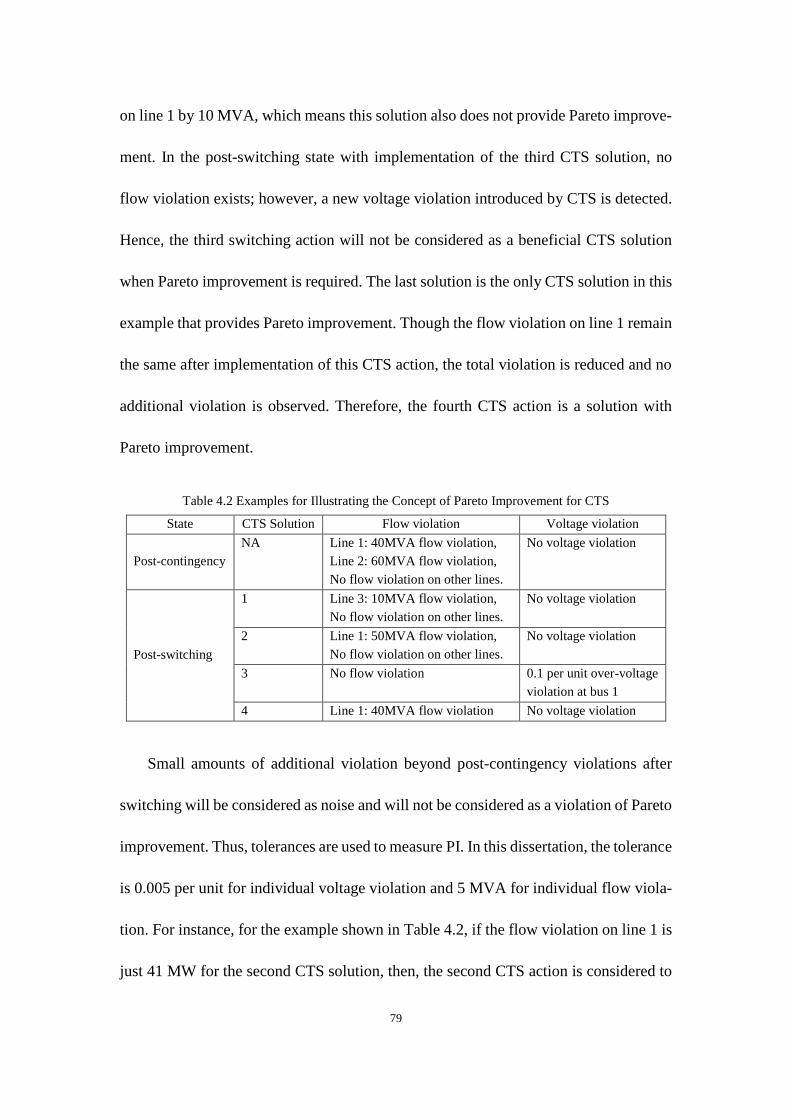
79

on line 1 by 10 MVA, which means this solution also does not provide Pareto improve-

ment. In the post-switching state with implementation of the third CTS solution, no

flow violation exists; however, a new voltage violation introduced by CTS is detected.

Hence, the third switching action will not be considered as a beneficial CTS solution

when Pareto improvement is required. The last solution is the only CTS solution in this

example that provides Pareto improvement. Though the flow violation on line 1 remain

the same after implementation of this CTS action, the total violation is reduced and no

additional violation is observed. Therefore, the fourth CTS action is a solution with

Pareto improvement.

Table 4.2 Examples for Illustrating the Concept of Pareto Improvement for CTS

State CTS Solution Flow violation Voltage violation

Post-contingency

NA Line 1: 40MVA flow violation,

Line 2: 60MVA flow violation,

No flow violation on other lines.

No voltage violation

Post-switching

1 Line 3: 10MVA flow violation,



2 Line 1: 50MVA flow violation,



3 No flow violation 0.1 per unit over-voltage

violation at bus 1

4 Line 1: 40MVA flow violation No voltage violation

Small amounts of additional violation beyond post-contingency violations after

switching will be considered as noise and will not be considered as a violation of Pareto

improvement. Thus, tolerances are used to measure PI. In this dissertation, the tolerance

is 0.005 per unit for individual voltage violation and 5 MVA for individual flow viola-

tion. For instance, for the example shown in Table 4.2, if the flow violation on line 1 is

just 41 MW for the second CTS solution, then, the second CTS action is considered to

80

be a beneficial solution that provides PI, since the additional 1 MW violation is within

the tolerance and thus is ignored.

4.2.3 Depth

In this dissertation, depth is proposed to estimate the effectiveness of the proposed

CTS algorithms. Depth is defined as the location of the identified beneficial switching

action in the candidate list for a particular contingency. It is worth mentioning that depth

is proposed to evaluate the efficiency of the proposed CTS algorithm rather than iden-

tifying a beneficial switching solution. The average depth can be calculated with the

equation below,

𝐷𝐶𝑇𝑆 =1

𝑀𝑐∑ 𝐿𝐶𝑇𝑆,𝑐𝑀𝑐𝑐=1 (4.3)

where 𝐿𝐶𝑇𝑆,𝑐 denotes the location of the CTS solution in the candidate list for contin-

gency 𝑐 and 𝑀𝑐 is the number of critical contingencies for which at least a beneficial

CTS solution exists.

4.3 Algorithms

Four heuristic algorithms are proposed in this dissertation to generate the candidate

switching list. They are listed below.

• Closest branches to contingency element (CBCE),

• Closest branches to violation element (CBVE),

• Regular Data mining (RDM),

• Enhanced Data Mining (EDM).

The beneficial switching branches are typically very close to the contingency ele-

ment or violation elements. Thus, two proximity based algorithms CBCE and CBVE

81

are proposed to create the candidate list. Inspired by the observation that the switching

branches come from a small subset of branches, RDM is proposed to generate the can-

didate CTS list. Customizing the candidate switching list for different contingencies

may substantially improve algorithm performance. Thus, EDM, an enhanced version

of RDM, is developed. Complete enumeration (CE) is also implemented in this disser-

tation as a benchmark to gauge the performance of the proposed heuristics.

4.3.1 CBCE and CBVE

Theoretically, the CBVE method may have a more robust performance than the

CBCE method. In the case of a branch contingency, the violations are very close to the

contingency branch. The candidate list of switching lines generated by CBCE would be

very similar to CBVE. Therefore, CBVE method would perform almost the same with

CBCE method. In the case of a generator contingency, it is possible that the violations

are far away from the contingency-generator since the generators including those that

are far from the contingency are re-dispatched. This may cause violations that are not

close to the contingency. In this case, the candidate list for CBCE may consist of

branches that are not near the violations and CBCE may not be able to relieve the vio-

lation. Therefore, CBVE would perform better than CBCE. In this dissertation, the

lengths of the candidate list for CBCE and CBVE are the same and each of the candidate

list consists of exactly 100 branches.

The distance of one element to another element used by CBCE and CBVE is the

number of branches in the shortest path connecting these two elements. The shortest

path has the smallest sum of the weights of its constituent branches. In this dissertation,

82

the weights of all branches are equal. Therefore, neither the electrical distance in ohms

nor the real distance in miles is involved. The proximity of two elements is only deter-

mined by the network topology, which makes it easy to implement the proposed algo-

rithms CBCE and CBVE.

4.3.2 RDM

Data mining method shows that beneficial switching actions are limited to a subset

of branches that can be determined by enumerating all possible switching actions on

the historical real-time EMS data. The candidate CTS list for a particular scenario con-

sists of the beneficial switching solutions identified in advance with other scenarios of

the same system. Tolerances can be used to filter out the solutions that provide trivial

benefits. Three different RDM methods with different tolerances are investigated in this

dissertation. They are referred to as RDM1, RDM2, and RDM3. No tolerance is applied

for RDM1; thus, even the CTS solution that provide negligible benefit will be listed as

a beneficial candidate. RDM2 uses 5% as the tolerance so that only the solutions that

provide more than 5% improvement will be considered as CTS candidates. RDM3 uses

10% as the tolerance; thus, the length of the candidate switching list for RDM3 is min-

imal, which would result in the least computational time.

The RDM method is examined only on the TVA system in this dissertation. Due

to the fact that only a very small number of the ERCOT cases are available, it is not

reasonable to conduct the RDM approach on the ERCOT system. The RDM algorithm

is also not performed on the PJM system due to the following two reasons: 1) it is

83

extremely time-consuming to identify the beneficial CTS solutions by performing com-

plete enumeration on all the 167 scenarios of the PJM system because of its large-scale

feature and computational challenge; 2) PJM real-time data have different network to-

pologies for different hours and it is extremely difficult to match the branch between

different hourly scenarios given that only very limited data are available.

For the TVA system, there are three days’ data or 72 cases that are divided into two

categories, training set and test set. The training set contains two days’ data while the

test set contains the other day’s data. CE is performed for each critical contingency on

the training cases and identifies the beneficial switching actions; those identified

switching actions form the candidate CTS list for the cases in the test set. Note that the

candidate CTS list is the same for different critical contingencies.

4.3.3 EDM

The candidate list of the RDM approach contains the same set of switching actions

for all the critical contingencies. However, this would unnecessarily make the list

lengthy and inefficient since the beneficial switching solutions for a contingency may

fail to reduce the violations caused by other contingencies.

A switching action that reduces the violation for a particular contingency in one

scenario may also provide benefits for the same contingency under a different scenario

but may not provide any benefit for other contingencies. Inspired by this idea, the EDM

approach that uses different candidate switching lists for different contingencies is pro-

posed. Similar to the regular data mining heuristic, the EDM heuristic is also a static

84

lookup table based approach. Though the switching list for each contingency is identi-

fied beforehand for both heuristics, EDM is much faster and more effective than RDM,

since the candidate switching list for EDM is customized for each contingency and is

much shorter than RDM.

PJM switching solutions as listed in [48] indicate that the beneficial switching so-

lutions for the same contingency would probably remain the same even if load profile

varies, which is consistent with the philosophy behind the proposed EDM approach.

The procedure for the EDM study in this dissertation consists of two stages. The

first stage is to determine the candidate switching actions using historical data in the

training set and the second stage is to investigate the performance of the EDM heuristic,

with the candidate CTS actions identified in the first stage, on different cases in the test

set.

Stage 1: Determination of Candidates CTS List

To illustrate the methodology of the proposed EDM heuristic, it is assumed that

multiple historical scenarios of the system conditions are available, which is reasonable

and practical for real power systems. These scenarios form the training set for deter-

mining the static lookup table offline. The associated procedure is described below:

1) For each scenario, RTCA is conducted to identify the critical contingencies.

2) For each critical contingency identified in step 1), complete enumeration of

all switchable branches is performed to determine the best switching action.

3) By examining all historical scenarios, a lookup table consisting of beneficial

switching solutions for the CTS application can then be created.

85

The lookup table contains the critical contingencies and the associated best CTS solu-

tions identified from the scenarios in the training set.

Fig. 4.4 shows the flowchart of the proposed EDM heuristic for the CTS applica-

tion. RTCA is conducted on the historical scenarios to identify critical contingencies

with potential violations. All the identified critical contingencies are sent to the CTS

routine along with all possible solutions in the candidate list. After this process is com-

pleted, the best CTS solutions for the same contingency in different scenarios can then

form the candidate switching list for the test cases that will be examined in stage 2.

Start

Scenario s in training set

Record the best CTS solution

for contingency c in scenario s

Run RTCA to determine critical contingencies Cs

Perform CE for critical contingency c in Cs

All critical contingencies in Cs

checked?

No

Yes

All scenarios in training set

examined?

No

End

Yes

Fig. 4.4 Flowchart of the Proposed EDM Heuristic.

Stage 2: Performance of the proposed EDM heuristic

Stage 2 investigates the performance of the proposed EDM heuristic by examining

the efficiency and effectiveness of the same CTS solutions, pre-determined for each

critical contingency in stage 1, on cases that are different with the historical scenarios

used in stage 1.

86

Similar to the RDM approach, only the TVA system is used to validate the effec-

tiveness of the EDM approach in this dissertation. The first two days or 48 hours that

represent the historical cases are used to determine the candidate switching list for each

critical contingency identified on those cases, which corresponds to stage 1. Then, those

pre-determined candidate lists are checked for the CTS performance on the remaining

24 cases in stage 2. The EDM heuristic that uses a candidate list without any tolerance

for improvement is referred to as EDM1. Candidate list with a tolerance of 5% is re-

ferred to as EDM2, while the list for EDM3 corresponds to a tolerance of 10%.

4.3.4 Complete Enumeration

Complete enumeration is implemented in this dissertation to evaluate the effective-

ness of the proposed heuristics. Complete enumeration can guarantee the optimal solu-

tion but that comes at the cost of a long solution time, which is not practical for real-

time applications. Thus, it is only used to provide a basis for evaluating the proposed

heuristics.

4.4 Case Studies

Numerical simulations are performed on the TVA, ERCOT, and PJM systems to

demonstrate the effectiveness of the proposed CTS algorithms for relieving the post-

contingency violations. The computer platform used in Section 4.4 is the same as the

computer used in Section 3.4. The simulations on the TVA system and the ERCOT

system are performed with only one single thread via a sequential program. Due to

computationally complexity, parallel computing with six threads is applied to solve the

PJM system.

87

Table 4.3 and Table 4.4 show the cumulative statistical results and the average

statistical results respectively. The results are associated with the first best switching

actions reported from the CBVE method without consideration of Pareto improvement.

The first best switching action is defined as the solution that the associated violation

reduction at an aggregate level is at least as good as the other candidates.

Table 4.3 Cumulative Statistics for the TVA, ERCOT, and PJM Systems

System # of sce-

narios

# of critical

contingencies

# of contingencies

with violations fully

eliminated by CTS

# of contingencies

with partial violation

reduced by CTS

# of contingencies

with no violation

reduced by CTS

TVA 72 4,272 427 (10.0%) 3,535 (82.7%) 310 (7.3%)

ERCOT 3 40 6 (15%) 27 (67.5%) 7 (17.5%)

PJM 167 8,064 2,684 (33.3%) 4,554 (56.5%) 826 (10.2%)

"Sum" 242 12,376 3,117 (25.2%) 8,116 (65.6%) 1,143 (9.2%)

Table 4.4 Average Statistics per Scenario

System # of sce-

narios

# of critical

contingencies

# of contingencies


eliminated by CTS

# of contingencies


reduced by CTS

# of contingencies

with no violation

reduced by CTS

TVA 72 59.3 5.9 49.1 4.3

ERCOT 3 13.3 2 9 2.3

PJM 167 48.3 16.1 27.3 4.9

The percentage values in the last column of Table 4.3 denote the ratios of critical

contingencies where there is no beneficial corrective switching action to the total num-

ber of critical contingencies. They are just around 7%, 18%, and 10% for the TVA,

ERCOT, and PJM systems respectively. The last row in Table 4.3 shows the statistics

over the three systems. The overall percent of critical contingencies that have no bene-

ficial CTS solutions is less than 10% among the three systems. The post-contingency

violations can be completely eliminated for over 25% of the critical contingencies iden-

tified for those three practical systems.

88

Note that there is no minimum threshold used for identifying beneficial CTS in

Table 4.3 and Table 4.4. Therefore, even the switching actions that provide negligible

improvement are considered. With 5% and 10% as the thresholds for determining the

beneficial CTS solutions, the associated results are shown in Table 4.5 and Table 4.6

respectively. With a threshold of 5%, the CTS solutions that provide less than 5% im-

provement will not be considered to be beneficial solutions and switching actions that

provide more than 95% improvement will be considered as the solutions that can fully

eliminate all the post-contingency violations. The statistics are calculated in the same

manner for a threshold of 10%. As the threshold increases from 0 to 10%, the number

of critical contingencies where the violations are fully eliminated with CTS increases,

as well as the number of critical contingencies where there is no beneficial solution.

Though the overall percent of critical contingencies for which at least a beneficial CTS

solution exists drops to 61% with a threshold of 10%, the application of CTS for post-

contingency violation reduction is still very promising.

Table 4.7 shows the average of violation reduction in percentage with CTS. The

results correspond to the first best switching solutions reported by the CBVE method.

The average reductions in flow violations are 40%, 53%, and 59% for the TVA, ER-

COT, and PJM systems respectively and the average reductions in voltage violations

are 36%, 12%, and 20% for those three systems respectively. Note that these statistics

are associated with the solutions that do not enforce Pareto improvement. If the CTS

solutions that do not provide Pareto improvement are ignored, only slight negligible

differences will be observed in those statistics. This implies that most CTS solutions

89

can reduce the violations at an aggregate level while each individual element is not

adversely affected.

Table 4.5 Cumulative Statistics per System with 5% Tolerance

System # of sce-

narios

# of critical

contingencies

# of contingencies


eliminated by CTS

# of contingencies


reduced by CTS

# of contingencies

with no violation

reduced by CTS

TVA 72 4,272 445 (10.4%) 2,962 (69.3%) 865 (20.2%)

ERCOT 3 40 9 (22.5%) 11 (27.5%) 20 (50.0%)

PJM 167 8,064 2,756 (34.2%) 2,049 (25.4%) 3,259 (40.4%)

"Sum" 242 12,376 3,210 (25.9%) 5022 (40.6%) 4144 (33.5%)

Table 4.6 Cumulative Statistics per System with 10% Tolerance

System # of sce-

narios

# of critical

contingencies

# of contingencies


eliminated by CTS

# of contingencies


reduced by CTS

# of contingencies

with no violation

reduced by CTS

TVA 72 4,272 458 (10.7%) 2,845 (66.6%) 969 (22.7%)

ERCOT 3 40 9 (22.5%) 8 (20.0%) 23 (57.5%)

PJM 167 8,064 2,802 (34.7%) 1,433 (17.8%) 3,829 (47.5%)

"Sum" 242 12,376 3,269 (26.4%) 4,286 (34.6%) 4,821 (39.0%)

Table 4.7 Average Violation Reduction with CTS per System

System

Average flow violation reduction Average voltage violation reduction

Without Pareto

improvement

With Pareto im-

provement

Without Pareto

improvement

With Pareto im-

provement

TVA 40.0% 40.0% 36.2% 35.6%

ERCOT 53.1% 49.3% 12.3% 12.3%

PJM 59.3% 59.0% 19.5% 19.3%

4.4.1 TVA Cases

Table 4.8 lists the results of various CTS methods on the TVA system. Note that

the results of the EDM heuristic are analyzed from a probabilistic view and are pre-

sented separately later in the same section.

Typically, it is expected that the CBCE method would perform similar to the CBVE

method. However, this is not the case for the TVA system since the majority of critical

contingencies are generator contingencies, which involve generation re-dispatch

90

throughout the entire network and cause violations that are far away from the contin-

gency element. This is the main reason why the results obtained from CBCE and CBVE

are so different. The CBVE method can reduce flow violations by 40%, which is very

close to what CE achieves. For the voltage violation reduction, it achieves around 36%

which is roughly 12% less than CE. However, the solution time for CBVE is less than

7% of the time that CE takes. The solution time for the CTS methods is averaged over

all the scenarios simulated and it does not include the solution time for RTCA. To be

consistent, the solution time for CTS is presented in the same manner throughout this

dissertation.

Table 4.8 Results of Various CTS Methods on the TVA System

CTS

methods

Average

solution

time (s)


Without Pareto

improvement

With Pareto

improvement

Without Pareto

improvement

With Pareto im-

provement

CBCE 166.7 15.6% 15.0% 31.8% 30.9%

CBVE 177.8 40.0% 40.0% 36.2% 35.6%

RDM1 201.9 40.6% 40.1% 48.1% 47.8%

RDM2 106.6 40.5% 40.0% 48.1% 47.7%

RDM3 98.3 40.5% 40.0% 48.0% 47.7%

CE 2585.3 40.8% 40.3% 48.2% 47.9%

Table 4.8 also presents the results obtained with the three RDM methods intro-

duced in Section 4.3. The RDM methods achieve almost the same results with CE while

the computational time is significantly reduced. The violation reductions with the three

RDM methods are very similar. However, RDM3 is the fastest since it has the shortest

list and it is 26 times faster than CE.

91

Table 4.9 shows the solution time of RTCA and various CTS methods on the TVA

system. The solution time that CBVE takes is about 4 times longer than the computa-

tional time of RTCA while RDM3 takes just twice the time that is required for perform-

ing RTCA. It is worth noting that RDM3 is over 50 times faster than CE for the case

that corresponds to the maximum solution time.

Table 4.9 Solution Time of RTCA and Various CTS Methods on the TVA System

Solution time (s)

Average Min Max

RTCA 45.0 43.4 47.7

CTS - CBCE 166.7 16.6 346.4

CTS - CBVE 177.8 17.7 373.0

CTS - RDM1 201.9 17.9 464.2

CTS - RDM2 106.6 9.9 230.8

CTS - RDM3 98.3 9.7 207.0

CTS - CE 2585.3 208.5 10523.7

Table 4.10 presents the statistics for violation reductions corresponding to the 5

best switching solutions with the CBVE heuristic. It is observed that the results with

and without enforcing Pareto improvement are very alike. This means that even if Pa-

reto improvement is not a requirement, most of the identified beneficial switching ac-

tions do not cause any additional violation while the total violations are reduced. The

average depth of the first best CTS solution for flow violation reduction is just 11,

which demonstrates that the beneficial switching elements are located very close to the

violation elements. For voltage violation, the average depths associated with the top 5

CTS solutions are similar and are around 40. This means that the heuristic algorithm

CBVE performs in a more effective way on the TVA system for flow violation reduc-

tion as compared to voltage violation reduction.

92

Fig. 4.5 shows the flow violation reductions and voltage violation reductions that

are associated with the top 5 CTS solutions identified by CBVE without imposing Pa-

reto improvement. The average flow violation reduction and average voltage violation

reduction are similar with the first best switching actions. However, the curve for volt-

age violation reduction is relatively flat while the flow violation reduction drops signif-

icantly as the rank of beneficial CTS solution decreases. Only top 2 CTS solutions iden-

tified for flow violation reduction provide improvement more than 15% while the fifth

best CTS solution for voltage violation reduction can achieve over 15% improvement.

Table 4.10 Results of the 5 Best Switching Actions on the TVA System using CBVE

CTS


Without Pareto

improvement

With Pareto im-

provement

Without Pareto

improvement

With Pareto im-

provement

Reduc-

tion Depth

Reduc-

tion Depth

Reduc-

tion Depth

Reduc-

tion Depth

1st Best 40.0% 11.0 40.0% 11.1 36.2% 46.1 35.6% 48.8

2nd Best 27.8% 23.9 27.7% 24.4 25.1% 46.1 24.8% 45.3

3rd Best 11.7% 54.0 11.7% 54.2 21.8% 39.3 21.6% 37.6

4th Best 8.6% 52.8 8.5% 52.9 19.5% 39.2 19.3% 38.8

5th Best 7.2% 47.8 7.2% 47.7 17.9% 39.9 17.7% 37.5

Analysis of Simulation in Stage 1 for EDM

With RTCA conducted on the scenarios of day 1 and day 2 for the TVA system,

153 different critical contingencies are identified. CE is performed on all 48 scenarios

to determine the best CTS solutions for each critical contingency. The best CTS solu-

tions for the same contingency under various historical scenarios in the training set form

the candidate list for that contingency.

Random variable 𝛼 is defined as the number of cases for which the same contin-

gency is identified as a critical contingency. Table 4.11 presents the statistics for this

93

random variable. From this table, it is observed that most of the critical contingencies

could cause violations for different system conditions corresponding to different his-

torical cases. In other words, a contingency that causes violations in one scenario may

also cause violations in other scenarios.

Fig. 4.5 Violation Reduction with the 5 Best Switching Actions Identified by CBVE on TVA.

Random variable 𝜏 is defined in (4.4). In (4.4), 𝛼𝑐 is number of cases where con-

tingency c is identified as a critical contingency and nT is the total number of cases

examined in this stage. nT is 48 in this dissertation. Thus, 𝜏 denotes the probability of

a contingency being identified as a critical contingency.

The statistics for 𝜏 is presented in Table 4.11. The maximum probability of a con-

tingency being identified as a critical contingency is as high as around 90%. The aver-

age number of scenarios in which the same contingency will be identified as a critical

contingency is 18.7 out of 48, corresponding to a probability of 39.0%.

40.0%

27.8%

11.7%

8.6%7.2%

36.2%

25.1%

21.8%19.5%

17.9%

0%

5%

10%

15%

20%

25%

30%

35%

40%

45%

1st 2nd 3rd 4th 5th

Aver

age

Vio

lati

on R

educt

ion

Best CTS solutions

Average Flow Violation Reduction

Average Voltage Violation Reduction

94

𝜏𝑐 = 𝛼𝑐 𝑛𝑇⁄ (4.4)

Table 4.11 Statistics for Random Variables 𝛼 and 𝜏

Max Min Median Average Standard deviation

𝛼 43 1 20 18.7 11.1

𝜏 89.6% 2.1% 41.7% 39.0% 23.1%

Fig. 4.6 shows the cumulative distribution function 𝐹𝜏 of variable 𝜏. It is observed

that the probability of a contingency being identified as a critical contingency, among

153 identified critical contingencies obtained in stage 1, is primarily in the range be-

tween 20% and 80%.

To verify the idea that the beneficial CTS solutions for a contingency will also

provide violation reduction for the same contingency in a different scenario of the sys-

tem, two random variables γ and β are proposed. Random variable γ denotes the number

of scenarios where a beneficial CTS solution exists for a critical contingency. Then β,

as defined in (4.5), denotes the probability that at least a beneficial CTS solution exists

for an identified critical contingency. The subscript c in (4.5) denotes critical contin-

gency c.

𝛽𝑐 =𝛾𝑐

𝛼𝑐× 100% (4.5)

Table 4.12 presents the statistics for random variable β. It shows that the probability

of existence of beneficial CTS solutions for a critical contingency is extremely high.

Even if 10% improvement is used as the tolerance for defining a beneficial switching

action, on average, beneficial CTS solutions are still available to relieve violations

caused by the same critical contingency for more than 80% of the scenarios.

95

0 20% 40% 60% 80% 100%

20%

40%

60%

80%

100%

0Cum

ula

tive

dis

trib

uti

on f

un

ctio

n

Probability of contingency

Fig. 4.6 Cumulative Distribution Function of Random Variable 𝜏.

Table 4.12 Statistics for Random Variable β

Heuristic Tolerance Max Min Median Average Standard deviation

EDM1 0 100% 0 100% 97.1% 13.84%

EDM2 5% 100% 0 100% 86.6% 29.0%

EDM3 10% 100% 0 100% 83.5% 31.3%

Random variable φ is defined as the number of switching actions in the candidate

list for a critical contingency. Table 4.13 presents the statistics for this random variable.

The candidate list obtained from EDM is extremely short. The average length is just

around two, which implies that the added computational time per contingency due to

CTS is just the solution time that is needed to perform two power flow simulations.

There are 153 numbers in the sample space for each random variable α, 𝜏, γ, β, and

φ since there were 153 critical contingencies identified in stage 1.

Table 4.13 Statistics for Random Variable φ

Tolerance Max Min Median Average Standard deviation

0 18 0 2 2.39 2.35

5% 6 0 1 1.66 0.99

10% 5 0 1 1.58 0.96

96

Analysis of Simulation in Stage 2 for EDM

Stage 2 aims to justify the proposed data-driven heuristic. Simulations were per-

formed on the 24 hourly scenarios of day 3 for the TVA system to demonstrate the

effectiveness of the proposed EDM approach. In this stage, RTCA is first conducted on

the 24 scenarios in the test set from day 3. Overall, 152 critical contingencies that would

cause network violations are identified. Among those critical contingencies identified

in stage 2, 84.2% or 128 contingencies are found in the critical contingency list identi-

fied from the 48 scenarios of day 1 and day 2 in the training set. For each critical con-

tingency in stage 2, only the beneficial switching actions identified in stage 1 for the

corresponding contingencies are examined for the proposed EDM heuristic.

Table 4.14 presents detailed statistics of the results obtained from RDM, EDM, and

CE methods respectively. The maximum, minimum, median, average, and standard de-

viation of the solution times per scenario for the different CTS methods are presented

in Table 4.14. For both RDM and EDM approaches, as the tolerance for defining ben-

eficial CTS solutions increases from 0% to 5%, the solutions time reduces by a large

factor while the violation reductions stay almost the same; however, further increase in

the tolerance from 5% to 10% only has a very small effect on the reduction in solution

time.

Both voltage violation reduction and flow violation reduction are reported in Table

4.14. Both RDM and EDM methods are proven to be very effective as they provide

almost the same violation reductions in comparison to the CE method. The violation

reductions obtained by the proposed EDM heuristic is only around 1% lower than the

97

RDM and CE methods, while EDM achieves the results in much less solution time.

EDM1 is around 20 times faster than RDM1 and EDM3 is over 10 times faster than

RDM3. Moreover, EDM is over 200 times faster than the CE method. In conclusion,

the proposed EDM heuristics provide near optimal solutions while adding the least

overhead to the solution time for contingency analysis, which is very promising for

real-time CTS applications.

Table 4.15 shows the average number of switching actions in the candidate list per

contingency and the average solution time for the CTS routine per scenario. In Table

4.15, nCTS denotes the average number of switching actions per contingency; and T1

denotes the average solution time of the CTS routine per scenario. It is observed that

the solution time is linearly correlated with the number of switching actions in the can-

didate list. Obviously, one reason why EDM is much faster than RDM is that the can-

didate list of the proposed EDM approach is much shorter.

Table 4.14 Results of the TVA Cases in the Third Day

Methods Solution times (s) Violation reduction

max min median average std Flow Voltage

RDM1 464.2 22.1 208.7 219.5 161.4 39.77% 51.09%

RDM2 225.9 11.0 103.6 108.3 79.5 39.77% 51.07%

RDM3 200.7 9.7 90.9 96.1 70.8 39.76% 50.95%

EDM1 20.9 1.5 10.7 11.1 7.5 38.74% 50.24%

EDM2 18.0 1.4 9.1 9.6 6.5 38.73% 50.22%

EDM3 17.6 1.1 8.9 9.3 6.3 38.73% 50.03%

CE 9636.5 208.5 2003.5 2458.2 2316.9 39.77% 51.22%

Table 4.15 Comparison among a Variety of CTS Methods on the TVA Cases in the Third Day

CE RDM1 RDM2 RDM3 EDM1 EDM2 EDM3

nCTS 1528.9 145.0 64.0 55.0 2.4 1.7 1.6

T1 (s) 2316.9 219.5 108.3 96.1 11.1 9.6 9.3

98

4.4.2 ERCOT Cases

Table 4.16 lists the results of various CTS approaches on the ERCOT system.

CBVE provides almost the same performance with CBCE in terms of voltage violation

reduction while it results in 10% more reduction in flow violation than CBCE. The

violation reductions achieved through those two heuristics are very similar to that

achieved with CE. However, the proposed heuristics are 47 times faster. Note that the

solution time is the average solution time for the three available scenarios of the ER-

COT system.

Table 4.16 Results of Various CTS Methods on the ERCOT System

CTS

methods

Average

solution

time (s)


Without Pareto

improvement

With Pareto

improvement

w/o Pareto im-

provement

w/ Pareto im-

provement

CBCE 245 40.8% 37.7% 12.1% 12.1%

CBVE 244 53.1% 49.3% 12.3% 12.3%

CE 11,505 53.3% 49.3% 14.3% 14.3%

Table 4.17 presents the average, minimum, and maximum solution times of RTCA

and different CTS heuristics. The overall solution times of the CTS heuristics are found

to be less than the time taken for RTCA since the number of critical contingencies that

require CTS is smaller for the ERCOT system compared to the TVA system. The max-

imum solution time to find the CTS actions is close to 6 minutes even for the sequential

implementation of the CTS heuristics. Note that the solution time of the proposed CTS

heuristics highly depends on the number of the identified critical contingencies. If all

contingencies in the contingency list are trivial, then CTS will not be implemented since

there will be no network violation and the associated solution time for CTS will just be

zero.

99

Table 4.17 Solution Time of RTCA and Various CTS Methods on the ERCOT System

Average (s) Min (s) Max (s)

RTCA 766.7 575.3 784.9

CTS - CBCE 244.8 181.5 356.1

CTS - CBVE 244.2 184.7 349.6

CTS - CE 11504.7 8728.3 16733.8

Fig. 4.7 shows violation reductions with the 5 best switching actions identified by

the CBVE algorithm on the ERCOT system. Pareto improvement is not imposed for

the results shown in Fig. 4.7. All top 5 switching actions can reduce the flow violations

significantly while the performance of CTS voltage violation reduction is less promis-

ing. The top CTS solutions can reduce the flow violations by 53.1% and even the fifth

best CTS solutions can reduce the flow violations by 47.2% on average. As for voltage

violation, the first best CTS solutions provide 12.3% improvement; however, the im-

provement provided by the second best CTS solutions is less than 10% on average and

the fifth best switching actions provide only 2.8% improvement which is negligible.

Fig. 4.7 Violation Reduction with the 5 Best Switching Actions on the ERCOT System.

53.1% 52.4%

49.2% 48.3% 47.2%

12.3%8.8%

5.2%4.2% 2.8%

0%

10%

20%

30%

40%

50%

60%

1st 2nd 3rd 4th 5th

Aver

age

Vio

lati

on R

educt

ion

Best CTS solutions



100

4.4.3 PJM Cases

Due to large-scale feature of the PJM system, the solution time for simulating

RTCA and CTS on the PJM system is significantly high. Thus, the PJM system is

solved with parallel computing using six threads rather than one single thread.

Table 4.18 shows the results obtained with CBCE and CBVE on the PJM system.

The flow violation reductions and voltage violation reductions achieved with CBCE

and CBVE are very similar. The solution times presented in Table 4.18 do not include

the time of RTCA and it is the average time over all 167 hourly scenarios. It is observed

from Table 4.19 that the average, minimum, and maximum solution times of those two

CTS heuristics are very similar.

Table 4.20 shows the statistics related to the 5 best switching actions identified by

the CBVE heuristic. The reductions in flow violations for the first and fifth best CTS

solutions are 59% and 46% respectively. However, for voltage violation, the reduction

ranges from 20% to 6% for the top 5 CTS solutions. All top 5 switching solutions pro-

vide substantial reduction for flow violation while only top 3 switching solutions pro-

vide reduction more than 10% for voltage violation. The depths of the beneficial CTS

solutions in the ranked candidate list are small for flow violation, which implies that

the beneficial switching branches are very close to the violation elements. The depths

of CTS that handles voltage violation are much larger than the depths of CTS that han-

dles flow violation, which indicates that the proximity-based heuristic is more efficient

for flow violation reduction than voltage violation reduction on the PJM system. The

101

violation reductions without Pareto improvement, obtained with CBVE, are presented

in Fig. 4.8.

Table 4.18 Results of Various CTS Methods on the PJM System

CTS

methods

Avg.

solution

time (s)


Without Pareto

improvement

With Pareto

improvement

Without Pareto

improvement

With Pareto

improvement

CBCE 1592.6 61.6% 60.2% 19.1% 18.8%

CBVE 1611.8 59.3% 59.0% 19.5% 19.3%

Table 4.19 Solution Times of RTCA and Various CTS Methods on the PJM System

Average (s) Min (s) Max (s)

RTCA 2617.3 2186.5 3100.1

CTS - CBCE 1592.6 236.9 3499.4

CTS - CBVE 1611.8 241.9 3441.1

Table 4.20 Results of the 5 Best Switching Actions on the PJM System using CBVE

CTS


Without Pareto im-

provement

With Pareto im-

provement

Without Pareto im-

provement

With Pareto im-

provement

Reduction Depth Reduction Depth Reduction Depth Reduction Depth

1st Best 59.3% 13.9 59.0% 14.4 19.5% 36.8 19.3% 37.6

2nd Best 57.7% 16.4 57.3% 16.7 14.6% 37.8 14.4% 38.1

3rd Best 52.6% 22.9 51.9% 23.7 11.5% 37.2 11.2% 37.9

4th Best 49.0% 26.5 48.7% 25.9 7.8% 39.9 7.7% 39.7

5th Best 46.3% 27.1 45.5% 27.4 6.4% 41.2 6.1% 41.4

102

Fig. 4.8 Violation Reduction with the 5 Best Switching Actions on the PJM System.

For the PJM system, the simulation for CE can take an extremely long time even

with 6 threads running in parallel. Therefore, CE is only performed on 6 selected sce-

narios out of 167 EMS snapshots. The 6 selected cases are hour 1, 5, 9, 13, 17, and hour

21 on day 1. They represent various system loading conditions for peak hours, off-peak

hours, and shoulder hours.

Table 4.21 shows the statistics for results obtained from CBCE, CBVE, and CE on

the selected scenarios of the PJM system. The heuristics achieve very similar results

with CE in terms of violation improvement. However, the two heuristics are approxi-

mately 110 times faster than the complete enumeration.

Table 4.21 Results of Various CTS Methods on the PJM System for the Selected Hours

CTS

Average

solution

time (s)


Without Pareto

improvement

With Pareto im-

provement

Without Pareto

improvement

With Pareto im-

provement

CBCE 872.3 62.1% 61.0% 19.4% 19.4%

CBVE 874.8 59.4% 59.4% 19.4% 19.4%

CE 96921.5 62.5% 62.5% 21.0% 20.4%

59.3% 57.7%

52.6%49.0%

46.3%

19.5%

14.6%11.5%

7.8% 6.4%

0%

10%

20%

30%

40%

50%

60%

70%

1st 2nd 3rd 4th 5th

Aver

age

Vio

lati

on R

educt

ion

Best CTS solutions



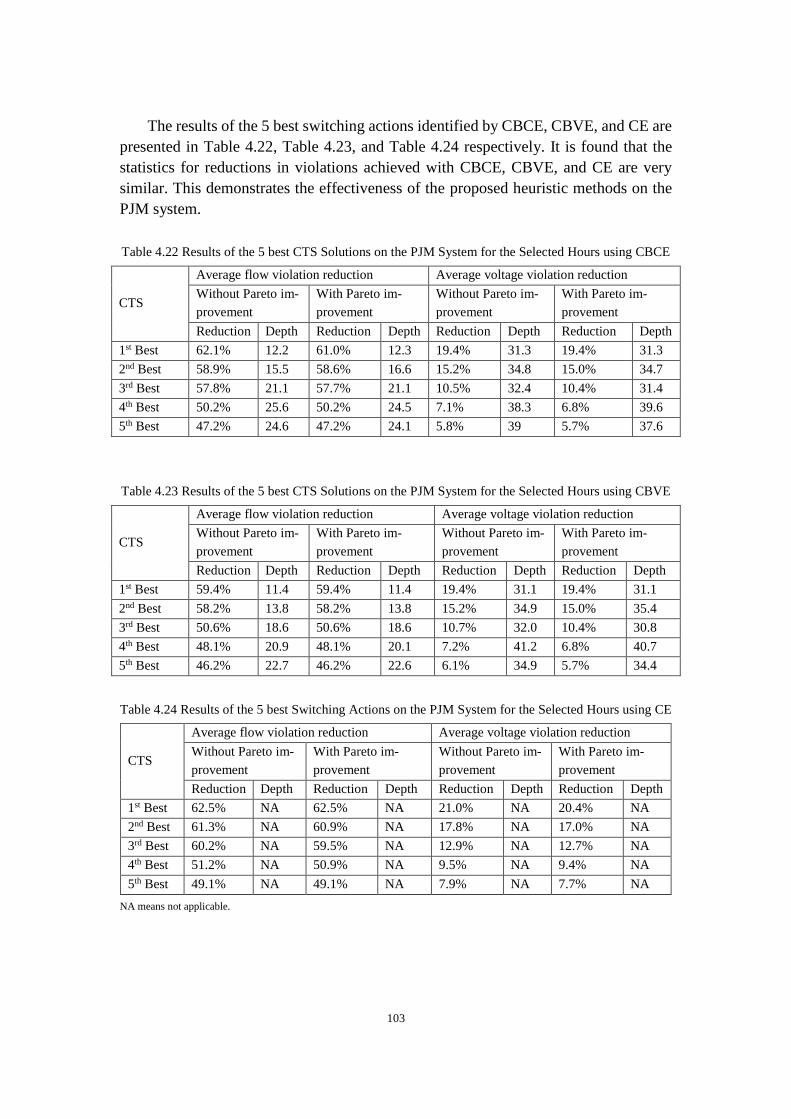
103

The results of the 5 best switching actions identified by CBCE, CBVE, and CE are

presented in Table 4.22, Table 4.23, and Table 4.24 respectively. It is found that the

statistics for reductions in violations achieved with CBCE, CBVE, and CE are very

similar. This demonstrates the effectiveness of the proposed heuristic methods on the

PJM system.

Table 4.22 Results of the 5 best CTS Solutions on the PJM System for the Selected Hours using CBCE

CTS


Without Pareto im-

provement

With Pareto im-

provement

Without Pareto im-

provement

With Pareto im-

provement


1st Best 62.1% 12.2 61.0% 12.3 19.4% 31.3 19.4% 31.3

2nd Best 58.9% 15.5 58.6% 16.6 15.2% 34.8 15.0% 34.7

3rd Best 57.8% 21.1 57.7% 21.1 10.5% 32.4 10.4% 31.4

4th Best 50.2% 25.6 50.2% 24.5 7.1% 38.3 6.8% 39.6

5th Best 47.2% 24.6 47.2% 24.1 5.8% 39 5.7% 37.6

Table 4.23 Results of the 5 best CTS Solutions on the PJM System for the Selected Hours using CBVE

CTS


Without Pareto im-

provement

With Pareto im-

provement

Without Pareto im-

provement

With Pareto im-

provement


1st Best 59.4% 11.4 59.4% 11.4 19.4% 31.1 19.4% 31.1

2nd Best 58.2% 13.8 58.2% 13.8 15.2% 34.9 15.0% 35.4

3rd Best 50.6% 18.6 50.6% 18.6 10.7% 32.0 10.4% 30.8

4th Best 48.1% 20.9 48.1% 20.1 7.2% 41.2 6.8% 40.7

5th Best 46.2% 22.7 46.2% 22.6 6.1% 34.9 5.7% 34.4

Table 4.24 Results of the 5 best Switching Actions on the PJM System for the Selected Hours using CE

CTS


Without Pareto im-

provement

With Pareto im-

provement

Without Pareto im-

provement

With Pareto im-

provement


1st Best 62.5% NA 62.5% NA 21.0% NA 20.4% NA

2nd Best 61.3% NA 60.9% NA 17.8% NA 17.0% NA

3rd Best 60.2% NA 59.5% NA 12.9% NA 12.7% NA

4th Best 51.2% NA 50.9% NA 9.5% NA 9.4% NA

5th Best 49.1% NA 49.1% NA 7.9% NA 7.7% NA

NA means not applicable.

104


Since the candidate switching list contains only 100 branches for CBVE and

CBCE, using more than 100 threads will be a waste of resources. Thus, up to 100

threads are used to investigate the efficiency of parallel computing with the proposed

CBVE and CBCE heuristics.

Table 4.25 lists the average CTS solution time with various threads on the TVA,

ERCOT, and PJM systems. To give a more intuitive understanding of how much time

can be reduced with multiple threads, the average CTS solution time with different

threads on the ERCOT system is shown in Fig. 4.9. It is clearly observed that the com-

puting time decreases as the number of threads used increases. Note that the solution

times shown in Table 4.25 and Fig. 4.9 are the average time over multiple scenarios for

the same system and thus are the average CTS solution time per system rather than the

average CTS solution time per contingency.

Table 4.25 Average CTS Solution Time per System with Different Threads

Average CTS solution time per system / s

# of threads 1 2 4 8 16 25 50 100

TVA 172.24 89.08 46.56 27.02 15.79 10.68 7.22 6.61

ERCOT 279.53 141.87 74.01 40.90 22.97 14.62 8.44 5.55

PJM NA NA NA 999.46 565.90 322.94 172.70 96.18

NA: not applicable

105

Fig. 4.9 Average CTS Solution Time per Scenario/Hour with Different Threads on the ERCOT System.

4.6 Conclusions

Violation reduction that can be achieved with CTS is studied in this chapter. Four

heuristic based CTS algorithms are proposed to determine the candidate switching list.

Numerical results on three large-scale practical systems demonstrate the effectiveness

of CTS for reducing post-contingency violations in an AC setting.

Promising results on the TVA system are obtained from the data mining methods,

RDM and EDM, in a reasonable solution time. All scenarios of the TVA system share

the same network topology. Thus, the performance of data mining methods on dynamic

network, for instance, caused by transmission maintenance outage, needs further inves-

tigations. Two other heuristic methods, CBCE and CBVE, have similar performance to

complete enumeration on the ERCOT system and the PJM system. However, CBCE

does not perform well on the TVA system while CBVE still shows a good performance.

The reason is that generation re-dispatch is conducted throughout the entire system for

0

50

100

150

200

250

300

1 2 4 8 16 25 50 100

So

luti

on

tim

e /

s

Number of threads

106

generator contingencies, which may cause violations that are far away from that the

contingency-generator and the candidate list generated from CBCE may not benefit the

system at all.

Complete enumeration is guaranteed to find the best solution. However, that comes

with the cost of a long computational time, which is impractical. Overall, CBVE heu-

ristic is considered to be the most efficient and robust CTS method among the proposed

heuristics in order to provide valid solutions for reducing post-contingency violations.

Based on the analysis on three large-scale practical power systems, the beneficial

switching solutions for flow violation reduction are typically found to be the overloaded

branches, or the branches that are in parallel or on the same path with the overloaded

branch. The reason for why CTS can reduce overloads without load shedding is that

CTS reconfigures the transmission network and transfers the flows on overloaded

branches to other paths that have extra available capacity. For voltage violation reduc-

tion, the identified CTS solutions typically carry a significant amount of reactive power

or have shunts connected to it. Thus, switching those CTS actions can change the reac-

tive power in the nearby area and, then change the voltage profile in the same area,

which may reduce over voltage violations or under voltage violations.

107

5. REAL-TIME SECURITY-CONSTRAINED ECONOMIC DIS-

PATCH WITH CORRECTIVE TRANSMISSION SWITCHING

Real-time security-constrained economic dispatch aims to provide the least cost

dispatch solution for the online generating units while meeting all system requirements

including network constraints. The system total operation cost includes energy cost and

reserve cost. No-load cost is not considered in RT SCED as it does not affect the results

at all. Typically, SCED uses the linearized DC power flow model rather than the AC

power flow model due to concerns regarding computational complexity and algorithm

convergence. In addition, RT SCED does not change generators’ status and network

topology. Thus, RT SCED is just a linear programming problem without any binary

variables and thus can be solved to optimality quickly if it is feasible.

The system monitoring function of EMS performs state estimation with the data

received from remote terminal units or local control center and determines the system

condition in real-time. Then, base-case power flow and RTCA execute and provide a

list of network constraints for RT SCED. This list of network constraints can be divided

into two categories: base-case network constraints (actual network constraints) and con-

tingency-case network constraints (potential network constraints). RT SCED considers

those two categories of network constraints as well as other requirements in its linear

optimization engine which will solve the associated problem and obtain a new set of

dispatch points that meet all requirements with minimum cost.

It is worth noting that RT SCED is based on the DC power flow model while base-

case power flow and contingency analysis use the full AC power flow model. Thus,

108

model conversion between RTCA and RT SCED is needed. This dissertation proposes

Procedure-A for connecting RTCA and RT SCED. The proposed Procedure-A is im-

plemented to mimic the industrial practice. Network constraints identified from base-

case power flow and RTCA are modeled in RT SCED.

Several SCED models are proposed and compared. To evaluate the quality of so-

lutions obtained from the different SCED models, SCED solutions are fed back to EMS

and then, base-case AC power flow and full AC contingency analysis are performed

again. The SCED model that has the best performance is selected. Simulation results

demonstrate the effectiveness of the proposed Procedure-A. It is observed that the so-

lution obtained from DC power flow model based SCED can pass AC feasibility check.

Due to network congestion, cheap generators may have to hold their power outputs,

which would result in significant congestion cost. As demonstrated in Chapter 4, CTS

can reduce post-contingency violations; in other words, CTS can relieve network con-

gestions. Therefore, as an enhanced version of Procedure-A, Procedure-B is proposed

to relieve congestions with CTS. With CTS, pseudo limits that are higher than the actual

limits can be used for the network constraints in the SCED model. The SCED using

pseudo limits in Procedure-B is referred to as enhanced SCED. With the use of pseudo

limits in E-SCED, the reliability benefits provided by CTS can be translated into sig-

nificant congestion cost savings due to substantially reduced need for expensive gener-

ation re-dispatch.

For solutions obtained from the proposed Procedure-B, branch overloads may be

observed under some critical contingencies in the post-SCED stage; this is because

109

pseudo limits that are higher than actual limits are used for the contingency-case net-

work constraints. However, the flow violations can be eliminated by implementing the

CTS solutions identified in the pre-SCED stage. Simulation results demonstrate the ef-

fectiveness of the proposed E-SCED approach as well as the proposed Procedure-B.

Voltage violations are typically handled locally. Moreover, SCED does not con-

sider voltage and reactive power. Therefore, in this chapter, RTCA focuses on flow

violations only. In addition, RTCA used in this chapter is performed only on transmis-

sion contingencies, which is consistent with existing industrial practice.

5.1 EMS Procedures

This section presents the proposed Procedure-A and Procedure-B in detail. In the

proposed Procedure-A, the network constraints formulated in DC model based RT

SCED are determined from AC model based RTCA; Procedure-A can perform model

conversion and connect RT SCED with the traditional RTCA. In fact, the proposed

Procedure-A represents existing industrial practice. Based on Procedure-A, Procedure-

B is proposed to utilize the flexibility in the transmission network. Procedure-B is a

procedure for connecting SCED with CTS-based RTCA.

Procedure-A uses the actual limits, calculated by RTCA, to enforce network con-

straints while higher pseudo limits are used in Procedure-B, which is the main differ-

ence between Procedure-A and Procedure-B. The pseudo limits are determined by

CTS-based RTCA. With the use of higher pseudo limits, the extra reliability provided

by CTS can then be captured in SCED and be translated into economic benefits.

110

Theoretically, the proposed Procedure-A can be replaced by an AC power flow

model based SCED model or ACOPF. However, AC based SCED is a non-linear and

non-convex problem and is extremely difficult to solve for large-scale real power sys-

tems in a limited time. In addition, convergence and robustness are also big concerns.

Therefore, the proposed Procedure-A, which is consistent with the industrial practice,

is preferred.

Theoretically, instead of using pseudo limits in E-SCED of the proposed Proce-

dure-B, CTS can be directly modeled in SCED and binary variables would be used to

indicate the status of switching element, which will convert SCED from an LP problem

into an MILP problem. This will cause a serious computational burden and substantially

increase the solution time. Therefore, directly modeling CTS in SCED is impractical

and Procedure-B with pseudo limits is preferred. In addition, the proposed Procedure-

B requires no change to existing tools and the solution time for SCED will not change

significantly.

Procedure-A and Procedure-B are presented in detail in Section 5.1.1 and Section

5.1.2 respectively. The detailed SCED mathematical models are presented in Section

5.2.

5.1.1 Procedure-A: SCED with RTCA

This section describes the proposed Procedure-A in detail. Fig. 5.1 illustrates the

flowchart of the proposed Procedure-A representing existing industrial practice. As

shown in Fig. 5.1, Procedure-A consists of four steps as listed below.

Step 1) Monitor system status.

111

Step 2) Perform base-case power flow and RTCA to determine the active net-

work constraints for SCED.

Step 3) Run SCED with the network constraints identified in Step 2).

Step 4) Evaluate the SCED solutions.

Start

Monitor System Status

Perform Base Case Power Flow

Perform RTCA

Record Network Constraints

Execute SCED

Evaluate the SCED Dispatch Points

End

Fig. 5.1 Flowchart of the Proposed Procedure-A for Connecting SCED with RTCA.

With the data collected from local control centers and remote terminal units in real-

time, state estimation is performed to determine the system status in Step 1). In Step 2),

with the starting point determined in Step 1), base-case power flow and RTCA are per-

formed sequentially; this step will identify the active network constraints that have to

be enforced in SCED for secure operations of power systems. Then, the SCED that is

subject to those active network constraints is solved and the optimal solution is reported

to operators. The last step of Procedure-A evaluates the SCED solution by rerunning

the base-case power flow and contingency analysis with the updated generators’ out-

puts; the contingency list simulated in this step is the same with Step 2).

112

Determination of Network Constraints

Due to large-scale feature of real power systems, it is impractical to model all con-

tingencies with all elements monitored in RT SCED. Thus, generation reserve is pro-

posed and modeled in RT SCED aiming to have extra backup power for handling con-

tingency in real-time and make sure the system is N-1 secure. However, reserve deliv-

erability cannot be guaranteed due to congestion. Thus, extra network constraints are

required to be enforced in RT SCED. With a limited number of extra network con-

straints modeled in SCED, it can still be solved within a short timeframe and be em-

ployed in real-time.

As described before, the network constraints can be divided into two categories,

actual base-case network constraints and potential contingency-case network con-

straints. Each base-case network constraint contains three items: transmission element

k under monitoring, initial active power flow 𝑃𝑘0 in the base case, and long-term normal

MW limit 𝐿𝑖𝑚𝑖𝑡𝐴𝑘 . Each contingency-case network constraint contains four items:

contingency element c, transmission element k under monitoring, initial active power

flow 𝑃𝑘,𝑐,0 under contingency c, and short-term emergency MW limit 𝐿𝑖𝑚𝑖𝑡𝐶𝑘𝑐 under

contingency c.

In reality, thermal limits for transmission elements are in the unit of MVA instead

of MW. However, approximate MW limits are used for SCED and they can be derived

by assuming that the reactive power flows do not change in the look-ahead period of

SCED. Then, the branch normal limit 𝐿𝑖𝑚𝑖𝑡𝐴𝑘 for base-case network constraint and

113

the emergency limit 𝐿𝑖𝑚𝑖𝑡𝐶𝑘𝑐 for contingency-case network constraint can be calcu-

lated by (5.1) and (5.2) respectively,

𝐿𝑖𝑚𝑖𝑡𝐴𝑘 = √𝑅𝑎𝑡𝑒𝐴2 − (max(|𝑄𝑘,𝑓𝑟𝑜𝑚|, |𝑄𝑘,𝑡𝑜|))2 (5.1)

𝐿𝑖𝑚𝑖𝑡𝐶𝑘𝑐 = √𝑅𝑎𝑡𝑒𝐶2 − (max(|𝑄𝑘𝑐,𝑓𝑟𝑜𝑚|, |𝑄𝑘𝑐,𝑡𝑜|))2 (5.2)

where 𝑄𝑘,𝑓𝑟𝑜𝑚 and 𝑄𝑘,𝑡𝑜 denote the reactive power on line k flowing out of from-bus

and to-bus in the base case respectively; 𝑄𝑘𝑐,𝑓𝑟𝑜𝑚 and 𝑄𝑘𝑐,𝑡𝑜 denote the reactive power

on line k flowing out of from-bus and to-bus under contingency c respectively.

In case that contingency analysis is not available, branch emergency limit 𝐿𝑖𝑚𝑖𝑡𝐶𝑘

under contingency can be approximately calculated by (5.3) which assumes reactive

power flows do not change under contingency,

𝐿𝑖𝑚𝑖𝑡𝐶𝑘 = √𝑅𝑎𝑡𝑒𝐶2 − (max(|𝑄𝑘,𝑓𝑟𝑜𝑚|, |𝑄𝑘,𝑡𝑜|))2 (5.3)

To reduce computational complexity, only a small subset of transmission elements

will be monitored. Active network constraints can be determined by comparing the

branch loading level with the tolerance 𝑃𝑐𝑡 for the base case or the tolerance 𝑃𝑐𝑡𝐶 for

the contingency cases. Tolerances 𝑃𝑐𝑡 and 𝑃𝑐𝑡𝐶 are pre-defined percentages with a

range between 0 and 100%. The branch loading level 𝐿𝐿𝑘 in the base case is defined in

(5.4) while the branch loading level 𝐿𝐿𝑘𝑐 under contingency c can be calculated with

(5.5),

𝐿𝐿𝑘 =max(|𝑆𝑘,𝑓𝑟𝑜𝑚|, |𝑆𝑘,𝑡𝑜|) /𝑅𝑎𝑡𝑒𝐴 (5.4)

𝐿𝐿𝑘𝑐 =max(|𝑆𝑘𝑐,𝑓𝑟𝑜𝑚|, |𝑆𝑘𝑐,𝑡𝑜|) /𝑅𝑎𝑡𝑒𝐶 (5.5)

114

where 𝑆𝑘,𝑓𝑟𝑜𝑚 and 𝑆𝑘,𝑡𝑜 denote the complex power on line k flowing out of from-bus

and to-bus in the base case respectively; 𝑆𝑘𝑐,𝑓𝑟𝑜𝑚 and 𝑆𝑘𝑐,𝑡𝑜 denote the complex power

on line k flowing out of from-bus and to-bus under contingency c respectively.

Therefore, a branch k will be monitored in the base case if its loading level 𝐿𝐿𝑘 is

greater than 𝑃𝑐𝑡. Similarly, a branch k will be monitored under contingency c if the

associated loading level 𝐿𝐿𝑘𝑐 is greater than 𝑃𝑐𝑡𝐶. Those monitored branch constraints

are referred to active network constraints. An active network constraint is referred to as

a critical network constraint if the associated flow exceeds the branch capacity. A con-

tingency is called active contingency if it causes one or multiple active network con-

straints. Similarly, a critical contingency is a contingency that would cause at least one

critical network constraint.

If 𝑃𝑐𝑡 is set to 1, only the actual congested and overloaded branches will be moni-

tored in the base case. Similarly, if 𝑃𝑐𝑡𝐶 is set to 1, then only the potential congested

and overloaded branches will be monitored under the associated contingencies.

The initial branch flow for base-case network constraints and contingency-case

network constraints that are modeled in SCED are determined by (5.6) and (5.7) re-

spectively,

𝑃𝑘0 = 𝑠𝑖𝑔𝑛(𝑃𝑘,𝑓𝑟𝑜𝑚) ∙ max(|𝑃𝑘,𝑓𝑟𝑜𝑚|, |𝑃𝑘,𝑡𝑜|) (5.6)

𝑃𝑘𝑐0 = 𝑠𝑖𝑔𝑛(𝑃𝑘𝑐,𝑓𝑟𝑜𝑚) ∙ max(|𝑃𝑘𝑐,𝑓𝑟𝑜𝑚|, |𝑃𝑘𝑐,𝑡𝑜|) (5.7)

where 𝑃𝑘,𝑓𝑟𝑜𝑚 and 𝑃𝑘,𝑡𝑜 denote the active power on line k flowing out of from-bus and

to-bus in base-case respectively; 𝑃𝑘𝑐,𝑓𝑟𝑜𝑚 and 𝑃𝑘𝑐,𝑡𝑜 denote the active power on line k

flowing out of from-bus and to-bus under contingency c respectively.

115

Representation of Transmission Losses

System losses in transmission network typically accounts for 2% to 4% of the total

demand. It would be impractical if all losses are picked up by slack bus. Thus, losses

should be precisely and properly modeled in SCED. Losses can either be modeled as

virtual loads or be calculated with loss coefficients. In this work, transmission losses

are not explicitly represented in the proposed SCED mathematical model; instead, vir-

tual loads are used to represent the transmission losses.

Multiple methods as listed below are available to convert losses in an AC model

into virtual loads in a DC model.

• assign losses to load buses,

• assign losses to generator buses,

• assign the loss on each branch to the actually receiving buses,

• assign the loss on each branch to the actually sending buses,

• assign the loss on each branch evenly to the from-bus and the to-bus.

In this work, the loss on each branch is evenly distributed to the two buses that are

connected to that branch and modeled as virtual loads. In addition, the losses are as-

sumed to remain the same. Note that, for the incremental PTDF based SCED models,

there is no need to model losses as virtual loads since they are already implicitly repre-

sented in those models.

5.1.2 Procedure-B: SCED with CTS based RTCA

The proposed Procedure-A, which represents the industrial practice for RT SCED,

is introduced in detail in Section 5.1.1. As demonstrated in Chapter 4, CTS is able to

116

enhance the system reliability by reducing violation under contingency. In this section,

Procedure-B is proposed to enhance Procedure-A by considering the benefits that are

provided by CTS. The proposed Procedure-B can substantially relieve network conges-

tion and significantly reduce the congestion cost as compared to Procedure-A. To dis-

tinguish the regular SCED in Procedure-A, the SCED that considers the effect of CTS

in Procedure-B is referred to as enhanced SCED.

The flowchart of the proposed Procedure-B is illustrated in Fig. 5.2. As shown in

Fig. 5.2, Procedure-B consists of six steps, which are listed below,

Step 1) Monitor system status.

Step 2) Perform base-case power flow and RTCA.

Step 3) Perform CTS on critical contingencies only and identify beneficial

switching actions for each critical contingency.

Step 4) Update the thermal limit in MW for critical network constraints.

Step 5) Run E-SCED and obtain a new set of dispatch points.

Step 6) Evaluate the E-SCED solution.

Start

Monitor System Status

Perform Base Case Power Flow

Perform RTCA

Record Network Constraints

Execute E-SCED

Evaluate the E-SCED Dispatch Points

End

Perform CTS Only on Critical Contingencies

Update MW Limit of Network Constraints

Fig. 5.2 Flowchart of the Proposed Procedure-B.

117

The first two steps of Procedure-B are the same as in Procedure-A. The third step

of Procedure-B is to perform CTS on critical contingencies only and identify switching

actions that can reduce post-contingency violations. Note that CTS is performed only

on critical contingencies aiming to relieve critical network constraints, which is time-

efficient as compared to that CTS is performed on all active contingencies. In Step 4),

the limits of critical network constraints are updated with (5.8) and details are provided

below.

For a critical contingency c, if the identified beneficial switching solutions can re-

duce the total violation and no single violation is worse off, then, the pseudo limit of

the associated constraint can be calculated by the equation presented below,

𝐿𝑖𝑚𝑖𝑡𝐶𝑘𝑐 = √(𝑅𝑎𝑡𝑒𝐶 + 𝑣𝑘𝑐𝑃𝑘𝑐,𝐶𝑇𝑆)2 − (max(|𝑄𝑘𝑐,𝑓𝑟𝑜𝑚|, |𝑄𝑘𝑐,𝑡𝑜|))2 (5.8)

where 𝑣𝑘𝑐 denotes the violation on branch k under contingency c and 𝑃𝑘𝑐,𝐶𝑇𝑆 denotes

the violation reduction in percent for branch k under contingency c with CTS and is

calculated by (5.9),

𝑃𝑘𝑐,𝐶𝑇𝑆 = (𝑣𝑘𝑐 − 𝑣𝑘𝑐,𝐶𝑇𝑆)/𝑣𝑘𝑐 (5.9)

where 𝑣𝑘𝑐,𝐶𝑇𝑆 is the violation on branch k under contingency c with CTS action imple-

mented.

In Step 5), E-SCED executes with the pseudo limits of critical network constraints

and then a new set of dispatch points for dispatchable units are obtained. The last step

of Procedure-B is to evaluate the E-SCED solutions. With the updated generation in the

post-SCED stage, RTCA is performed on the same contingencies with Step 2) and it

118

will probably report violations as higher pseudo limits are used in E-SCED rather than

the actual limits; however, those post-contingency violations are expected to occur on

the same element under the same contingencies that are reported by RTCA in the pre-

SCED stage. For the critical contingencies causing those post-contingency violations,

the beneficial CTS solutions identified in Step 3) in the pre-SCED stage are also ex-

pected to reduce violations under the same contingencies in the post-SCED stage, which

is demonstrated in Section 5.3.

5.2 SCED Mathematical Formulation

A SCED mathematical model is first proposed in this section, followed by several

model variants. Based on availability of network flow information and different forms

of network constraints, five SCED models are proposed in this dissertation. They are

cold-start PTDF based SCED, warm-start PTDF based SCED, hot-start PTDF based

SCED, cold-start B-𝜃 based SCED, and hot-start B-𝜃 based SCED.

The proposed SCED models co-optimize energy and reserve simultaneously while

enforcing physical restrictions such as power balance constraints and security require-

ments such as reserve requirements.

Load shedding is included in both the base case and the contingency cases to handle

the potential infeasibility and prevent the SCED software from terminating without re-

porting any information. Load shedding is modeled as slack variables in the power bal-

ance constraints.

119

It is worth mentioning that in the commercial RT SCED tools used by ISOs, all

constraints are relaxed with slack variables; for different set of slack variables, the pen-

alty factors for the associated penalty terms in objective function can be different as

different types of constraints to be enforced have different priorities. Thus, the ISOs’

commercial RT SCED tools will not terminate even in the worst case; instead, they can

inform operators of what may be the sources causing SCED infeasibility and enable

operators to manually adjust the system to avoid any potential damage.

5.2.1 Unit Cost Curve

ISOs including PJM, MISO, and NYISO typically require generators to submit in-

cremental energy offer that is represented by MW quantity and price pairs [143]-[145].

For instance, both MISO and PJM accept up to 10 price-quantity segments. There are

two types of energy offers: slope cost curve and block cost curve.

Fig. 5.3 shows an example that illustrates the unit block incremental cost curve.

The lengths of the three segments are 𝑃𝑔,𝑠1, (𝑃𝑔,𝑠2 − 𝑃𝑔,𝑠1), and (𝑃𝑔,𝑠3 − 𝑃𝑔,𝑠2) while

the associated constant costs are C1, C2, and C3 respectively. 𝑝𝑔1, 𝑝𝑔2, and 𝑝𝑔3 denotes

the net MW outputs associated with segment 1, 2, and 3 respectively. For the same

generator, the optimal SCED solution will not schedule any power outputs on a segment

if any other segment with a lower price is not entirely selected since the objective func-

tion is to minimize the total cost.

Fig. 5.4 illustrates the unit slope incremental cost curve. Obviously, the costs of the

second segment and third segment are not constant, which would create non-linearity

120

when calculating the total cost. As non-linearity may create computational issues, line-

arization of the slope cost curve is required. The slope cost curve can be divided into

several block sub-segments with the same length and, then, the total cost of a slope

segment can be calculated by summing up those block sub-segments. Fig. 5.5 illustrates

the linearization of a slope segment.

The procedure for linearizing a slope segment is presented below.

1) determine the number of sub-segments,

𝑛𝑆𝑆 = 𝑟𝑜𝑢𝑛𝑑(𝑃𝑔,𝑠2−𝑃𝑔,𝑠1

∆𝑏𝑖) (5.10)

where 𝑛𝑆𝑆 denotes the number of sub-segments for a slope segment; ∆𝑏𝑖 denotes the

initially selected breadth of a sub-segment; and round(x) is a function that returns the

integer number that is closest to x.

2) calculate the sub-segment breadth with (5.11),

∆𝑠 = (𝑃𝑔,𝑠2 − 𝑃𝑔,𝑠1)/𝑛𝑆𝑆 (5.11)

where ∆𝑠 denotes the actual breadth of each sub-segment.

3) the cost for each sub-segment can be determined by (5.12).

𝐶𝑖 = 𝐶1 + (𝑖 − 0.5)(𝑃𝑔,𝑠2−𝑃𝑔,𝑠1)

(𝐶2−𝐶1)∆𝑠,𝑖 = 1. . 𝑛𝑆𝑆 (5.12)

With the above procedure, a slope segment that is not flat can be converted into a

series of small block segments. Therefore, a slope cost curve can be converted into a

block cost curve, which enables the objective function to maintain linearity. It is worth

noting that for both block cost curves and slope cost curves, the first segment is flat

with zero slope and probably corresponds to the generator economic minimum 𝑃𝑔,𝑠1

and the no-load cost C1.

121

Pg (MW)

Price ($/MWh)

Segment 1 Segment 2 Segment 3

C1

C2

C3

Pg,s10 Pg,s2 Pg,s3

pg1

pg2

pg3

Fig. 5.3 Block Cost Curve of Generator g.

Pg (MW)

Price ($/MWh)

Segment 1 Segment 2 Segment 3

C1

C2

C3

Pg,s10 Pg,s2 Pg,s3

pg1

pg2

pg3

Fig. 5.4 Slope Cost Curve of Generator g.

Segment 2

Pg,s1 Pg,s2

pg2

...

...

...

s s s s

Fig. 5.5 Illustration of Linearization of a Slope Segment.

122

5.2.2 Objective Function

The proposed SCED models share the same objective function as existing industry

practice, which is to minimize the total cost including operating energy cost and reserve

cost. The objective function used in this work is shown below,

𝑚𝑖𝑛 ∑ ∑ 𝑝𝑔,𝑖 ∙ 𝐶𝑔,𝑖𝑁𝑆𝑔𝑖=1𝑔∈𝐺𝐷 + ∑ 𝑠𝑟𝑔 ∙ 𝐶𝑆𝑅𝑔𝑔∈𝐺 + 𝑃𝐹_𝑃𝐷𝑠ℎ𝑒𝑑 ∙ (∑ 𝑝𝑑,𝑠ℎ𝑒𝑑𝑑∈𝐷 +

∑ ∑ 𝑝𝑑,𝑠ℎ𝑒𝑑,𝑐𝑑∈𝐷𝑐∈𝐶 ) (5.13)

Note that slope cost curves are converted into block cost curves before solving

SCED.

5.2.3 Constraints

The constraints of a basic SCED can be expressed by (5.14)-(5.37). There are five

sets of constraints: power balance constraints, load shedding constraints, generators

constraints, reserve constraints, and network constraints. Those types of constraints are

first introduced below and then several alternative constraints are presented.

Power Balance Constraints

One single system-wide power balance constraint per scenario is enough to model

the power balance constraint for the PTDF based SCED formulation. System-wide

power balance between generation and demand are enforced in (5.14) and (5.15) for the

base case and the contingency cases respectively. For B-𝜃 power flow model based

formulation, node power balance constraints are used instead of one single system-wide

constraint, which will be introduced later in this section.

∑ 𝑝𝑔𝑔∈𝐺 = ∑ (𝑃𝑑 − 𝑝𝑑,𝑠ℎ𝑒𝑑)𝑑∈𝐷 (5.14)

∑ 𝑝𝑔,𝑐𝑔∈𝐺 = ∑ (𝑃𝑑 − 𝑝𝑑,𝑠ℎ𝑒𝑑,𝑐)𝑑∈𝐷 , 𝑐 ∈ C (5.15)

123

Load Shedding Constraints

In a real power system, negative load may be used in the EMS to model fixed flows

on the tie lines from energy market solutions. It is not reasonable to shed loads that are

used to represent tie-line transfer flows with other neighboring systems. Similarly, it is

not right to shed virtual loads that are used to represent losses. Thus, shedding load on

negative loads and virtual loads is not allowed in this work, which is guaranteed by

(5.16) and (5.17). For an actual positive demand, the shedded load cannot exceed the

amount of that demand, which is guaranteed by (5.18) and (5.19).

𝑝𝑑,𝑠ℎ𝑒𝑑 = 0, 𝑑 ∈ {DN, DV} (5.16)

𝑝𝑑,𝑠ℎ𝑒𝑑,𝑐 = 0,𝑑 ∈ {DN, DV}, 𝑐 ∈ C (5.17)

0 ≤ 𝑝𝑑,𝑠ℎ𝑒𝑑 ≤ 𝑃𝑑 , 𝑑 ∈ {D}\{DN, DV} (5.18)

0 ≤ 𝑝𝑑,𝑠ℎ𝑒𝑑,𝑐 ≤ 𝑃𝑑 ,𝑑 ∈ {D}\{DN, DV}, 𝑐 ∈ C (5.19)

Generator Constraints

Some generators such as self-scheduling units in practical power systems may not

be available for dispatch to system operators. Therefore, those generators’ outputs are

fixed in RT SCED, which is expressed with (5.20) and (5.21).

Dispatchable generators typically offer stepwise incremental cost curves that con-

sist of one or multiple pairs of segment prices and segment lengths. Equation (5.22)

ensures that a generator’s output equals the summation of the power outputs on all seg-

ments. Constraint (5.23) can guarantee that the power scheduled for each segment will

not exceed the associated segment breadth.

124

Constraints (5.24) and (5.25) enforce the active power outputs of generators to be

within their upper limits as well as lower limits for the base case and contingency cases

respectively. Generators’ energy ramping limit is modeled in (5.26) while generators’

spinning ramping restriction is enforced by (5.27). Note that the ramping rates for en-

ergy re-dispatch and reserve deployment for the same unit may be different.

𝑝𝑔 = 𝑃𝑔0, 𝑔 ∈ (𝐺 − 𝐺𝐷) (5.20)

𝑝𝑔,𝑐 = 𝑃𝑔0, 𝑔 ∈ (𝐺 − 𝐺𝐷), 𝑐 ∈ C (5.21)

𝑝𝑔 = ∑ 𝑝𝑔,𝑖𝑁𝑆𝑔𝑖=1

, 𝑔 ∈ 𝐺𝐷 (5.22)

0 ≤ 𝑝𝑔,𝑖 ≤ 𝐵𝑆𝑔,𝑖, 𝑔 ∈ 𝐺𝐷 (5.23)

𝑃𝑔,𝑚𝑖𝑛 ≤ 𝑝𝑔 ≤ 𝑃𝑔,𝑚𝑎𝑥,𝑔 ∈ 𝐺 (5.24)

𝑃𝑔,𝑚𝑖𝑛 ≤ 𝑝𝑔,𝑐 ≤ 𝑃𝑔,𝑚𝑎𝑥,𝑔 ∈ 𝐺, 𝑐 ∈ C (5.25)

−𝑀𝑅𝑅𝑔 ∙ 𝑇𝐸𝐷 ≤ 𝑝𝑔 − 𝑃𝑔0 ≤ 𝑀𝑅𝑅𝑔 ∙ 𝑇𝐸𝐷,𝑔 ∈ 𝐺 (5.26)

−𝑆𝑅𝑅𝑔 ∙ 𝑇𝑆𝑅 ≤ 𝑝𝑔,𝑐 − 𝑝𝑔 ≤ 𝑆𝑅𝑅𝑔 ∙ 𝑇𝑆𝑅,𝑔 ∈ 𝐺, 𝑐 ∈ C (5.27)

Reserve Constraints

The spinning reserve that an online unit can provide is subject to its ramping capa-

bility, which is expressed in (5.28). Constraint (5.29) guarantees that the sum of a unit’s

output and reserve cannot exceed its maximum limit. In other words, reserve is also

restricted by unit’s available capacity in addition to ramping limit. The “largest gener-

ator” rule is used for the reserve requirements as defined in (5.30), which ensures that

there would be enough reserve to cover any of loss of a single generation.

0 ≤ 𝑠𝑟𝑔 ≤ 𝑆𝑅𝑅𝑔 ∙ 𝑇𝑆𝑅,∀𝑔 ∈ 𝐺 (5.28)

𝑝𝑔 + 𝑠𝑟𝑔 ≤ 𝑃𝑔,𝑚𝑎𝑥,∀𝑔 ∈ 𝐺 (5.29)

125

∑ 𝑠𝑟𝑔𝑔∈𝐺 ≥ 𝑝𝑔 + 𝑠𝑟𝑔,∀𝑔 ∈ 𝐺 (5.30)

Network Constraints

Though the largest generator contingency reserve requirement is modeled in

SCED, there may still exist potential network violations due to congestion which limits

reserve deliverability. Thus, it is necessary to model active network constraints in

SCED. Branch thermal limits for the base case and contingency cases are enforced in

(5.31) and (5.32) respectively. The branch monitor sets can be different for the base

case and different contingency cases.

Due to concerns regarding voltage stability and transient stability, the total transfer

capacity of the ties connecting two areas cannot exceed a specific limit which is referred

to as interface limit or transfer limit. In SCED, the stability limit can be addressed by

including constraints on the sum of active power flows on the branches that form the

interface. The interface limit constraints are represented by (5.33) and (5.34) for the

base case and contingency cases respectively. Note that the interface limit under con-

tingency may be different with the limit in the base case especially when the contin-

gency element is one of branches forming that interface.

Equations (5.35) and (5.36) that are used to calculate branch flows take the effects

of generation re-dispatch, load shedding, and demand fluctuation into account. Note

that (5.31) and (5.32) are only for branches in the monitor sets and (5.33) and (5.34) are

only for critical interfaces; however, (5.35) and (5.36) are for both branches in the mon-

itor sets and branches forming the active interfaces. The flow on contingency branch c

is forced to be zero via (5.37).

126

−𝐿𝑖𝑚𝑖𝑡𝐴𝑘 ≤ 𝑝𝑘 ≤ 𝐿𝑖𝑚𝑖𝑡𝐴𝑘, 𝑘 ∈ 𝐾𝑀(0) (5.31)

−𝐿𝑖𝑚𝑖𝑡𝐶𝑘 ≤ 𝑝𝑘,𝑐 ≤ 𝐿𝑖𝑚𝑖𝑡𝐶𝑘, 𝑘 ∈ KM(c), 𝑐 ∈ C (5.32)

∑ 𝑝𝑘𝑘∈𝐾𝐼(𝑖) ≤ 𝐿𝑖𝑚𝑖𝑡𝑖, 𝑖 ∈ 𝐼𝑀(0) (5.33)

∑ 𝑝𝑘,𝑐𝑘∈𝐾𝐼(𝑖) ≤ 𝐿𝑖𝑚𝑖𝑡𝑖𝑐, 𝑖 ∈ 𝐼𝑀(𝑐), 𝑐 ∈ C (5.34)

𝑝𝑘 = 𝑃𝑘0 + ∑ (𝑃𝑇𝐷𝐹𝑛,𝑘 ∙ (∑ (𝑝𝑔 − 𝑃𝑔0)𝑔∈𝐺(𝑛) + ∑ (𝑝𝑑,𝑠ℎ𝑒𝑑 + 𝑃𝑑0 −𝑑∈𝐷(𝑛)𝑛∈𝑁

𝑃𝑑))) ,𝑘 ∈ {𝐾𝑀(0), 𝐼𝐾𝑀(0)} (5.35)

𝑝𝑘,𝑐 = 𝑃𝑘0 + 𝐿𝑂𝐷𝐹𝑘,𝑐 ∙ 𝑃𝑐0 + ∑ (𝑂𝑇𝐷𝐹𝑛,𝑘,𝑐 ∙ (∑ (𝑝𝑔,𝑐 − 𝑃𝑔0)𝑔∈𝐺(𝑛) +𝑛∈𝑁

∑ (𝑝𝑑,𝑠ℎ𝑒𝑑,𝑐 + 𝑃𝑑0 − 𝑃𝑑)𝑑∈𝐷(𝑛) )) , 𝑘 ∈ {𝐾𝑀(𝑐), 𝐼𝐾𝑀(𝑐)}\{𝑐}, 𝑐 ∈ C (5.36)

𝑝𝑘,𝑐 = 0, 𝑘 ∈ {𝑐}, 𝑐 ∈ C (5.37)

Alternative Constraints

Constraints (5.14)-(5.37) along with the objective function (5.13) form a basic

SCED mathematical model. Enhancement can be made to this model. Some of those

constraints can be replaced with alternative constraints as illustrated below.

Adding 𝑃𝑔0 to each expression in inequality constraint (5.26) would reformulate it

to (5.38), which shares the same form with (5.24). By simply taking the minimum of

upper limits for 𝑝𝑔 as the new upper limit and using the maximum of lower limits for

𝑝𝑔 as the new lower limit, constraints (5.38) and (5.24) can be combined as (5.39). In

other words, constraints (5.24) and (5.26) can be replaced by one single constraint

(5.39), which would reduce the number of constraints and may increase the perfor-

mance in terms of computational time.

𝑃𝑔0 −𝑀𝑅𝑅𝑔 ∙ 𝑇𝐸𝐷 ≤ 𝑝𝑔 ≤ 𝑃𝑔0 +𝑀𝑅𝑅𝑔 ∙ 𝑇𝐸𝐷,𝑔 ∈ 𝐺 (5.38)

127

max{𝑃𝑔0 −𝑀𝑅𝑅𝑔 ∙ 𝑇𝐸𝐷 , 𝑃𝑔,𝑚𝑖𝑛} ≤ 𝑝𝑔 ≤ min{𝑃𝑔0 +𝑀𝑅𝑅𝑔 ∙ 𝑇𝐸𝐷 , 𝑃𝑔,𝑚𝑎𝑥} , 𝑔 ∈ 𝐺

(5.39)

When branch reactive power flow under contingency is available, 𝐿𝑖𝑚𝑖𝑡𝐶𝑘𝑐 can be

calculated by (5.2) and should replace 𝐿𝑖𝑚𝑖𝑡𝐶𝑘 in (5.32). Thus, (5.32) would be con-

verted into the constraint shown below.

−𝐿𝑖𝑚𝑖𝑡𝐶𝑘,𝑐 ≤ 𝑝𝑘,𝑐 ≤ 𝐿𝑖𝑚𝑖𝑡𝐶𝑘,𝑐, 𝑘 ∈ KM(c), 𝑐 ∈ C (5.40)

Similarly, if the initial branch flow 𝑃𝑘,𝑐,0 under contingency c is available from

contingency analysis, the model would be more accurate by replacing 𝑃𝑘0 +

𝐿𝑂𝐷𝐹𝑘,𝑐𝑃𝑐0 with 𝑃𝑘,𝑐,0 in (5.36). Thus, (5.36) can be replaced by (5.41).

𝑝𝑘,𝑐 = 𝑃𝑘,𝑐,0 + ∑ (𝑂𝑇𝐷𝐹𝑛,𝑘,𝑐 ∙ (∑ (𝑝𝑔,𝑐 − 𝑃𝑔0)𝑔∈𝐺(𝑛) + ∑ (𝑝𝑑,𝑠ℎ𝑒𝑑,𝑐 + 𝑃𝑑0 −𝑑∈𝐷(𝑛)𝑛∈𝑁

𝑃𝑑))) , 𝑘 ∈ {𝐾𝑀(𝑐), 𝐼𝐾𝑀(𝑐)}\{𝑐}, 𝑐 ∈ C (5.41)

If the initial branch flow for both the base case and contingency case are not avail-

able, then, incremental PTDF based equations (5.35) and (5.36) can be replaced by

cold-start PTDF based equations (5.42) and (5.43) respectively.

𝑝𝑘 = ∑ (𝑃𝑇𝐷𝐹𝑛,𝑘 ∙ (∑ 𝑝𝑔𝑔∈𝐺(𝑛) + ∑ (𝑝𝑑,𝑠ℎ𝑒𝑑 − 𝑃𝑑)𝑑∈𝐷(𝑛) )𝑛∈𝑁 , 𝑘 ∈

{𝐾𝑀(0), 𝐼𝐾𝑀(0)} (5.42)

𝑝𝑘,𝑐 = ∑ (𝑂𝑇𝐷𝐹𝑛,𝑘,𝑐 ∙ (∑ 𝑝𝑔,𝑐𝑔∈𝐺(𝑛) + ∑ (𝑝𝑑,𝑠ℎ𝑒𝑑,𝑐 − 𝑃𝑑)𝑑∈𝐷(𝑛) ))𝑛∈𝑁 , 𝑘 ∈

{𝐾𝑀(𝑐), 𝐼𝐾𝑀(𝑐)}\{𝑐}, 𝑐 ∈ C (5.43)

Instead of using PTDF formulation, calculation of branch flow can use B-θ formu-

lation, which are defined in (5.44) and (5.45). It is worth mentioning that all branch

flows have to be calculated with B-θ formulation because there are mutual effects be-

tween voltage angle θ of all buses, while only the flows on branches of interests need

128

to be calculated with PTDF formulation. With B-θ formulation being used in SCED,

system-wide power balance constraints (5.14) and (5.15) should be replaced with node

power balance constraints (5.46) and (5.47) respectively.

𝑝𝑘 = (𝛿𝑛(𝑘−) − 𝛿𝑛(𝑘+) + 𝛼𝑘)/𝑋𝑘, 𝑘 ∈ 𝐾 (5.44)

𝑝𝑘,𝑐 = (𝛿𝑛(𝑘−),𝑐 − 𝛿𝑛(𝑘+),𝑐 + 𝛼𝑘)/𝑋𝑘, 𝑘 ∈ 𝐾\{𝑐}, 𝑐 ∈ C (5.45)

∑ 𝑝𝑔𝑔∈𝐺(𝑛) + ∑ 𝑝𝑘𝑘∈𝐾(𝑛+) − ∑ 𝑝𝑘𝑘∈𝐾(𝑛−) = ∑ (𝑃𝑑 − 𝑝𝑑,𝑠ℎ𝑒𝑑)𝑑∈𝐷(𝑛) , 𝑛 ∈ 𝑁 (5.46)

∑ 𝑝𝑔,𝑐𝑔∈𝐺(𝑛) + ∑ 𝑝𝑘,𝑐𝑘∈𝐾(𝑛+) − ∑ 𝑝𝑘,𝑐𝑘∈𝐾(𝑛−) = ∑ (𝑃𝑑 − 𝑝𝑑,𝑠ℎ𝑒𝑑,𝑐)𝑑∈𝐷(𝑛) , 𝑛 ∈ 𝑁,

𝑐 ∈ C (5.47)

5.2.4 Models

Based on the availability of network flow information and different power flow

formulations, five different SCED models are proposed in this dissertation. They are

listed below:

• Model 1: hot-start PTDF based SCED model,

• Model 2: warm-start PTDF based SCED model,

• Model 3: cold-start PTDF based SCED model,

• Model 4: hot-start B-𝜃 based SCED model,

• Model 5: cold-start B-𝜃 based SCED model.

The first three SCED models use PTDF power flow formulation while B-𝜃 power flow

formulation is used in the last two SCED models.

There are two types of SCED: corrective SCED (CSCED) and preventive SCED

(PSCED). Generation re-dispatch is allowed for CSCED in the post-contingency sce-

129

narios; in other words, with CSCED model, the generation dispatch points under con-

tingency are not necessary to be the same with the base-case generation schedule. How-

ever, the base-case generation schedule remains the same for all contingency cases with

PSCED model. PSCED repositions online generators in advance to satisfy the opera-

tional requirements in both the base case and contingency cases. Therefore, PSCED is

more conservative than CSCED, which would result in high variable operation cost.

However, PSCED can provide a more secure and reliable solution than CSCED as the

solution obtained from PSCED can withhold the loss of a single contingency without

adjustment. Most, if not all, ISOs implement PSCED model rather than CSCED model

due to security concerns.

Corrective SCED Models

The constraints described in Section 5.2.3 are general constraints for CSCED as

variable 𝑝𝑔,𝑐 is defined and used to represent unit generation under various contingency

scenarios. The five proposed SCED models with corrective control strategy are de-

scribed in Table 5.1. Those proposed SCED models share most of the constraints. For

instance, the three SCED models that use PTDF formulation share the same system-

wide power balance constraints while the two SCED models that use B-𝜃 formulation

share the same node power balance constraints.

The initial branch flow 𝑃𝑘,𝑐,0 under contingency and the emergency limit 𝐿𝑖𝑚𝑖𝑡𝐶𝑘𝑐

that can be obtained from RTCA are available to Model 1, while Model 2 uses 𝑃𝑘,0 and

line outage distribution factor (LODF) to calculate branch flow under contingency and

uses 𝐿𝑖𝑚𝑖𝑡𝐶𝑘 as the emergency limits of all contingency-case network constraints. A

130

cold-start branch flow calculation formulation is used in Model 3 rather than the incre-

mental branch flow calculation formulations used in Model 1 and Model 2. SCED is

built on the linearized DC power flow model; thus, apart from model error, the error of

PTDF based branch flow calculation also depends on unit generation. Model 3 uses the

entire generator output to calculate branch flow; however, incremental models only use

the change in generator output, which is typically much smaller than the entire genera-

tor output, to calculate branch flow. Thus, the model precision of Model 3 would be

less than Model 1 and Model 2. Model 4 and Model 5 are based on traditional B-𝜃

power flow model. The difference between them is that Model 4 uses customized

𝐿𝑖𝑚𝑖𝑡𝐶𝑘𝑐 as the emergency limits for different contingency cases while Model 5 uses

𝐿𝑖𝑚𝑖𝑡𝐶𝑘 as the emergency limit for all modeled active contingencies.

Table 5.1 Multiple Corrective SCED Models

Shared set of

constraints

Power balance

constraints Network constraints

CSCED Model 1 (5.16)-(5.23),

(5.25),

(5.27)-(5.31),

(5.33), (5.34),

(5.37), (5.39)

(5.14), (5.15)

(5.35), (5.40), (5.41)

CSCED Model 2 (5.32), (5.35), (5.36)

CSCED Model 3 (5.32), (5.42), (5.43)

CSCED Model 4 (5.46), (5.47)

(5.40), (5.44), (5.45)

CSCED Model 5 (5.32), (5.44), (5.45)

Preventive SCED Models

Corrective SCED allows the units’ outputs under contingency to deviate from the

base-case dispatch point, which would result in cheaper cost than preventive SCED.

However, due to security and reliability concerns, preventive SCED is more popular in

industry than corrective SCED. This section illustrates the mathematical model for

SCED using preventive control strategy.

131

Given a CSCED model, a simple way to form a PSCED model is to add one more

set of constraints (5.48), which force units’ outputs under contingency to remain the

same with units’ outputs in the base case, into that CSCED model.

𝑝𝑔,𝑐 = 𝑝𝑔,𝑔 ∈ 𝐺,𝑐 ∈ 𝐶 (5.48)

To construct a concise PSCED formulation, (5.48) can be simply substituted into

the constraints that are involved with 𝑝𝑔,𝑐. Thus, with adjustment, constraints (5.15),

(5.36), (5.41), (5.43), and (5.47) can be transformed into the constraints below, (5.49)

through (5.53), respectively. Moreover, with (5.48), constraints (5.21) and (5.25) will

be equivalent to (5.20) and (5.24) respectively and constraint (5.27) will definitely hold;

therefore, constraints (5.21), (5.25), and (5.27) should be removed in the PSCED model.

∑ 𝑝𝑑,𝑠ℎ𝑒𝑑𝑑∈𝐷 = ∑ 𝑝𝑑,𝑠ℎ𝑒𝑑,𝑐𝑑∈𝐷 , 𝑐 ∈ C (5.49)

𝑝𝑘,𝑐 = 𝑃𝑘0 + 𝐿𝑂𝐷𝐹𝑘,𝑐𝑃𝑐0 + ∑ (𝑂𝑇𝐷𝐹𝑛,𝑘,𝑐(∑ (𝑝𝑔 − 𝑃𝑔0)𝑔∈𝐺(𝑛) +𝑛∈𝑁

∑ (𝑝𝑑,𝑠ℎ𝑒𝑑,𝑐 + 𝑃𝑑0 − 𝑃𝑑)𝑑∈𝐷(𝑛) )) , 𝑘 ∈ {𝐾𝑀(𝑐), 𝐼𝐾𝑀(𝑐)}\{𝑐}, 𝑐 ∈ C (5.50)

𝑝𝑘,𝑐 = 𝑃𝑘,𝑐,0 + ∑ (𝑂𝑇𝐷𝐹𝑛,𝑘,𝑐(∑ (𝑝𝑔 − 𝑃𝑔0)𝑔∈𝐺(𝑛) + ∑ (𝑝𝑑,𝑠ℎ𝑒𝑑,𝑐 + 𝑃𝑑0 −𝑑∈𝐷(𝑛)𝑛∈𝑁

𝑃𝑑))) , 𝑘 ∈ {𝐾𝑀(𝑐), 𝐼𝐾𝑀(𝑐)}\{𝑐}, 𝑐 ∈ C (5.51)

𝑝𝑘,𝑐 = ∑ (𝑂𝑇𝐷𝐹𝑛,𝑘,𝑐(∑ 𝑝𝑔𝑔∈𝐺(𝑛) + ∑ (𝑝𝑑,𝑠ℎ𝑒𝑑,𝑐 − 𝑃𝑑)𝑑∈𝐷(𝑛) ))𝑛∈𝑁 , 𝑘 ∈

{𝐾𝑀(𝑐), 𝐼𝐾𝑀(𝑐)}\{𝑐}, 𝑐 ∈ C (5.52)

∑ 𝑝𝑔𝑔∈𝐺(𝑛) + ∑ 𝑝𝑘,𝑐𝑘∈𝐾(𝑛+) − ∑ 𝑝𝑘,𝑐𝑘∈𝐾(𝑛−) = ∑ (𝑃𝑑 − 𝑝𝑑,𝑠ℎ𝑒𝑑,𝑐)𝑑∈𝐷(𝑛) , 𝑛 ∈ 𝑁, 𝑐 ∈ C

(5.53)

132

To further reduce the problem complexity, contingency-case load shedding varia-

ble 𝑝𝑑,𝑠ℎ𝑒𝑑,𝑐 can be replaced by base-case load shedding variable 𝑝𝑑,𝑠ℎ𝑒𝑑. Thus, con-

straints (5.17), (5.19), and (5.49) can be ignore and constraints (5.50)-(5.53) can be

converted to the constraints listed below, (5.54)-(5.57), respectively.

𝑝𝑘,𝑐 = 𝑃𝑘0 + 𝐿𝑂𝐷𝐹𝑘,𝑐𝑃𝑐0 + ∑ (𝑂𝑇𝐷𝐹𝑛,𝑘,𝑐(∑ (𝑝𝑔 − 𝑃𝑔0)𝑔∈𝐺(𝑛) +𝑛∈𝑁

∑ (𝑝𝑑,𝑠ℎ𝑒𝑑 + 𝑃𝑑0 − 𝑃𝑑)𝑑∈𝐷(𝑛) )) , 𝑘 ∈ {𝐾𝑀(𝑐), 𝐼𝐾𝑀(𝑐)}\{𝑐}, 𝑐 ∈ C (5.54)

𝑝𝑘,𝑐 = 𝑃𝑘,𝑐,0 + ∑ (𝑂𝑇𝐷𝐹𝑛,𝑘,𝑐(∑ (𝑝𝑔 − 𝑃𝑔0)𝑔∈𝐺(𝑛) + ∑ (𝑝𝑑,𝑠ℎ𝑒𝑑 + 𝑃𝑑0 −𝑑∈𝐷(𝑛)𝑛∈𝑁

𝑃𝑑))) , 𝑘 ∈ {𝐾𝑀(𝑐), 𝐼𝐾𝑀(𝑐)}\{𝑐}, 𝑐 ∈ C (5.55)

𝑝𝑘,𝑐 = ∑ (𝑂𝑇𝐷𝐹𝑛,𝑘,𝑐(∑ 𝑝𝑔𝑔∈𝐺(𝑛) + ∑ (𝑝𝑑,𝑠ℎ𝑒𝑑 − 𝑃𝑑)𝑑∈𝐷(𝑛) ))𝑛∈𝑁 ,𝑘 ∈

{𝐾𝑀(𝑐), 𝐼𝐾𝑀(𝑐)}\{𝑐}, 𝑐 ∈ C (5.56)

∑ 𝑝𝑔𝑔∈𝐺(𝑛) + ∑ 𝑝𝑘,𝑐𝑘∈𝐾(𝑛+) − ∑ 𝑝𝑘,𝑐𝑘∈𝐾(𝑛−) = ∑ (𝑃𝑑 − 𝑝𝑑,𝑠ℎ𝑒𝑑)𝑑∈𝐷(𝑛) , 𝑛 ∈ 𝑁, 𝑐 ∈ C

(5.57)

Table 5.2 Multiple Preventive SCED Models

Shared set of constraints Power balance constraints Network constraints

PSCED Model 1 (5.16), (5.18), (5.20),

(5.22), (5.23), (5.28)-

(5.31), (5.33), (5.34),

(5.37) (5.39)

(5.14)

(5.35), (5.40), (5.55)

PSCED Model 2 (5.32), (5.35), (5.54)

PSCED Model 3 (5.32), (5.42), (5.56)

PSCED Model 4 (5.46), (5.57)

(5.40), (5.44), (5.45)

PSCED Model 5 (5.32), (5.44), (5.45)

Similar to the proposed CSCED models, the proposed SCED models with preven-

tive control strategy are described in Table 5.2. The differences between the proposed

PSCED models are the availability of network flow information and different branch

flow calculation formulations, which are consistent with the differences between the

proposed CSCED models.

133

5.2.5 Market Implication

In addition to providing updated real-time dispatch solutions, SCED is also used to

determine real-time energy market solutions including LMP. As the proposed E-SCED

takes advantage of transmission network flexibility by using pseudo limit rather than

actual limit used by a traditional SCED, it is important to analyze the effect of utiliza-

tion of pseudo limit on market results. Thus, LMP, load payment, generator revenue,

generator cost, generator rent, congestion cost, and congestion revenue are introduced

and analyzed in this work.

Locational marginal pricing is a market mechanism that is used to clear wholesale

energy markets that are managed by ISOs. A locational marginal price at a specific bus

reflects the least cost of supplying the next increment load at that bus while meeting all

physical and reliability constraints. LMP consists of three components: energy compo-

nent, congestion component, and loss component. If a system had a network with infi-

nite capacity and no losses, all LMPs would be the same over the entire system. How-

ever, in reality, losses cannot be avoided and network congestion issue typically exists.

In this work, losses are represented by virtual loads for SCED models 3-5 and are im-

plicitly incorporated in the initial branch flows for SCED models 1-2; thus, the loss

component is ignored in this work. The nodal LMP for PSCED model 1 can be calcu-

lated by the following equation,

𝐿𝑀𝑃𝑛 = 𝐿𝑀𝑃𝑠 + 𝐿𝑀𝑃𝑐𝑔,𝑛, 𝑛 ∈ 𝑁 (5.58)

where 𝐿𝑀𝑃𝑐𝑔,𝑛 denotes the congestion component of the LMP at bus n, which can be

calculated below,

134

𝐿𝑀𝑃𝑐𝑔,𝑛 = ∑ 𝑃𝑇𝐷𝐹𝑛,𝑘(𝐹𝑘+ − 𝐹𝑘

−)𝑘∈𝐾𝑀(0) +∑ ∑ 𝑂𝑇𝐷𝐹𝑛,𝑘,𝑐(𝐹𝑘,𝑐+ − 𝐹𝑘,𝑐

− )𝑘∈𝐾𝑀(𝑐)𝑐∈𝐶 +

∑ ∑ 𝑃𝑇𝐷𝐹𝑛,𝑘(𝐹𝑖+ − 𝐹𝑖

−)𝑘∈𝐾𝐼(𝑖)𝑖∈𝐼𝑀(0) + ∑ ∑ ∑ 𝑂𝑇𝐷𝐹𝑛,𝑘,𝑐(𝐹𝑖,𝑐+ −𝑘∈𝐾𝐼(𝑖)𝑖∈𝐼𝑀(0)𝑐∈𝐶

𝐹𝑖,𝑐− ) , 𝑛 ∈ 𝑁 (5.59)

Proof of (5.58)

This proof is only for deriving the nodal LMP equation (5.58); thus, for simplicity,

the constraints and variables that are not of interest are ignored, as well as the objective

function. As strong duality theory is used to prove (5.58), the constraints for a simpli-

fied but sufficient primal problem are listed below.

∑ 𝑃𝐼𝑛𝑛∈𝑁 = 0 (𝐿𝑀𝑃𝑠) (5.60)

∑ 𝑝𝑔𝑔∈𝐺(𝑛) + ∑ 𝑝𝑑,𝑠ℎ𝑒𝑑𝑑∈𝐷(𝑛) − 𝑃𝐼𝑛 = ∑ 𝑃𝑑𝑑∈𝐷(𝑛) , 𝑛 ∈ 𝑁 (𝐿𝑀𝑃𝑛) (5.61)

𝑃𝑘0 + ∑ (𝑃𝑇𝐷𝐹𝑛,𝑘(𝑃𝐼𝑛 − 𝑃𝐼𝑛,0))𝑛∈𝑁 ≤ 𝐿𝑖𝑚𝑖𝑡𝐴𝑘 , 𝑘 ∈ 𝐾𝑀(0) (𝐹𝑘+) (5.62)

−𝑃𝑘0 − ∑ (𝑃𝑇𝐷𝐹𝑛,𝑘(𝑃𝐼𝑛 − 𝑃𝐼𝑛,0))𝑛∈𝑁 ≤ 𝐿𝑖𝑚𝑖𝑡𝐴𝑘, 𝑘 ∈ 𝐾𝑀(0) (𝐹𝑘−) (5.63)

𝑃𝑘,𝑐,0 + ∑ (𝑂𝑇𝐷𝐹𝑛,𝑘(𝑃𝐼𝑛 − 𝑃𝐼𝑛,0))𝑛∈𝑁 ≤ 𝐿𝑖𝑚𝑖𝑡𝐶𝑘𝑐, 𝑘 ∈ 𝐾𝑀(𝑐) (𝐹𝑘,𝑐+ ) (5.64)

−𝑃𝑘,𝑐,0 − ∑ (𝑂𝑇𝐷𝐹𝑛,𝑘(𝑃𝐼𝑛 − 𝑃𝐼𝑛,0))𝑛∈𝑁 ≤ 𝐿𝑖𝑚𝑖𝑡𝐶𝑘𝑐, 𝑘 ∈ 𝐾𝑀(𝑐) (𝐹𝑘,𝑐− ) (5.65)

∑ (𝑃𝑘0 + ∑ (𝑃𝑇𝐷𝐹𝑛,𝑘(𝑃𝐼𝑛 − 𝑃𝐼𝑛,0)𝑛∈𝑁 )𝑘∈𝐾𝐼(𝑖) ≤ 𝐿𝑖𝑚𝑖𝑡𝑖, 𝑖 ∈ 𝐼𝑀(0) (𝐹𝑖+) (5.66)

−∑ (𝑃𝑘0 + ∑ (𝑃𝑇𝐷𝐹𝑛,𝑘(𝑃𝐼𝑛 − 𝑃𝐼𝑛,0)𝑛∈𝑁 )𝑘∈𝐾𝐼(𝑖) ≤ 𝐿𝑖𝑚𝑖𝑡𝑖, 𝑖 ∈ 𝐼𝑀(0) (𝐹𝑖−) (5.67)

∑ (𝑃𝑘,𝑐,0 + ∑ (𝑂𝑇𝐷𝐹𝑛,𝑘(𝑃𝐼𝑛 − 𝑃𝐼𝑛,0)𝑛∈𝑁 )𝑘∈𝐾𝐼(𝑖) ≤ 𝐿𝑖𝑚𝑖𝑡𝑖𝑐, 𝑖 ∈ 𝐼𝑀(𝑐) (𝐹𝑖,𝑐+ ) (5.68)

−∑ (𝑃𝑘,𝑐,0 + ∑ (𝑂𝑇𝐷𝐹𝑛,𝑘(𝑃𝐼𝑛 − 𝑃𝐼𝑛,0)𝑛∈𝑁 )𝑘∈𝐾𝐼(𝑖) ≤ 𝐿𝑖𝑚𝑖𝑡𝑖𝑐, 𝑖 ∈ 𝐼𝑀(𝑐) (𝐹𝑖,𝑐− ) (5.69)

Constraint (5.60) ensures the system-wide power balance while constraint (5.61) is

for nodal power balance. Constraint (5.60) is redundant for B-θ based SCED (SCED

model 4 - SCED model 5) while constraint (5.61) is not needed for PTDF based SCED

135

(SCED model 1 - SCED model 3); however, they are listed in this model just for deriv-

ing the relationship between nodal LMP and system LMP. Constraints (5.62)-(5.65)

show that the system is subject to branch thermal limit. Moreover, power systems are

also restricted by interface limits, which is guaranteed by (5.66)-(5.69). Variables

𝐿𝑀𝑃𝑠, 𝐿𝑀𝑃𝑛, 𝐹𝑘+, 𝐹𝑘

− 𝐹𝑘,𝑐+ , 𝐹𝑘,𝑐

− , 𝐹𝑖+, 𝐹𝑖

−, 𝐹𝑖,𝑐+ , and 𝐹𝑖,𝑐

− are the dual variables that are as-

sociated with these constraints of the primal problem.

Note that variable 𝑃𝐼𝑛 denotes power net injection at bus n, which can either posi-

tive or non-positive; then, it is unconstrained in the primal problem. Therefore, the as-

sociated constraints in the dual problem are the equality constraints as expressed in

(5.70),

𝐿𝑀𝑃𝑛 − 𝐿𝑀𝑃𝑠 + ∑ 𝑃𝑇𝐷𝐹𝑛,𝑘(𝐹𝑘+ − 𝐹𝑘

−)𝑘∈𝐾𝑀(0) + ∑ ∑ 𝑂𝑇𝐷𝐹𝑛,𝑘,𝑐(𝐹𝑘,𝑐+ −𝑘∈𝐾𝑀(𝑐)𝑐∈𝐶

𝐹𝑘,𝑐− ) + ∑ ∑ 𝑃𝑇𝐷𝐹𝑛,𝑘(𝐹𝑖

+ − 𝐹𝑖−)𝑘∈𝐾𝐼(𝑖)𝑖∈𝐼𝑀(0) +

∑ ∑ ∑ 𝑂𝑇𝐷𝐹𝑛,𝑘,𝑐(𝐹𝑖,𝑐+ − 𝐹𝑖,𝑐

− )𝑘∈𝐾𝐼(𝑖)𝑖∈𝐼𝑀(0)𝑐∈𝐶 = 0, 𝑛 ∈ 𝑁 (5.70)

where 𝐿𝑀𝑃𝑠 and 𝐿𝑀𝑃𝑛 are unconstrained; 𝐹𝑘+, 𝐹𝑘

− 𝐹𝑘,𝑐+ , 𝐹𝑘,𝑐

− , 𝐹𝑖+, 𝐹𝑖

−, 𝐹𝑖,𝑐+ , and 𝐹𝑖,𝑐

− are

non-positive. Then, (5.58) can be obtained by reformatting (5.70).

Average LMP is proposed to analyze the effect of modeling CTS implicitly in

SCED on LMP. Average LMP over the entire system is defined in (5.71). Similarly,

average congestion LMP is defined in (5.72).

𝐴𝑣𝑔𝐿𝑀𝑃 = ∑ 𝐿𝑀𝑃𝑛𝑛∈𝑁 , 𝑛 ∈ 𝑁 (5.71)

𝐴𝑣𝑔𝐿𝑀𝑃𝑐𝑔 = ∑ 𝐿𝑀𝑃𝑐𝑔,𝑛𝑛∈𝑁 , 𝑛 ∈ 𝑁 (5.72)

136

Load payment is calculated by (5.73) and generator revenue is determined by

(5.74). Equation (5.75) calculates the generator cost which is part of the objective func-

tion. Generator rent is calculated by (5.76). Note that in this work, the generator rent

only accounts energy and does not include reserve rent. Congestion revenue, which is

used to fund the financial transmission rights markets, is the difference between gener-

ator revenue and load payment, as calculated by (5.77).

𝐿𝑑𝑃𝑎𝑦𝑚𝑡 = ∑ (𝐿𝑀𝑃𝑛(∑ 𝑃𝑑)𝑑∈𝐷(𝑛) )𝑛∈𝑁 (5.73)

𝐺𝑒𝑛𝑅𝑣𝑛 = ∑ (𝐿𝑀𝑃𝑛(∑ 𝑝𝑔𝑔∈𝐺(𝑛) ))𝑛∈𝑁 (5.74)

𝐺𝑒𝑛𝐶𝑜𝑠𝑡 = ∑ ∑ 𝑝𝑔,𝑖𝐶𝑔,𝑖𝑁𝑆𝑔𝑖=1𝑔∈𝐺𝐷 (5.75)

𝐺𝑒𝑛𝑅𝑒𝑛𝑡 = 𝐺𝑒𝑛𝑅𝑣𝑛 − 𝐺𝑒𝑛𝐶𝑜𝑠𝑡 (5.76)

𝐶𝑛𝑔𝑠𝑡𝑅𝑣𝑛 = 𝐺𝑒𝑛𝑅𝑣𝑛 − 𝐺𝑒𝑛𝐶𝑜𝑠𝑡 (5.77)

In addition to congestion revenue, congestion cost is also proposed to measure the

degree of network congestion. Congestion cost is defined as (5.78),

𝐶𝑛𝑔𝑠𝑡𝐶𝑜𝑠𝑡 = 𝑇𝑜𝑡𝑎𝑙𝐶𝑜𝑠𝑡1 − 𝑇𝑜𝑡𝑎𝑙𝐶𝑜𝑠𝑡2 (5.78)

where 𝑇𝑜𝑡𝑎𝑙𝐶𝑜𝑠𝑡1 denotes the optimal objective value of either an E-SCED or a SCED

and 𝑇𝑜𝑡𝑎𝑙𝐶𝑜𝑠𝑡2 denotes the optimal objective value obtained by solving the same E-

SCED or SCED but without any network constraints.

Thus, the congestion cost reduction 𝐶𝐶𝑅𝐶𝑇𝑆 achieved by E-SCED as compared to

a traditional SCED can be calculated with (5.79).

𝐶𝐶𝑅𝐶𝑇𝑆 = 𝐶𝑛𝑔𝑠𝑡𝐶𝑜𝑠𝑡𝐸−𝑆𝐶𝐸𝐷 − 𝐶𝑛𝑔𝑠𝑡𝐶𝑜𝑠𝑡𝑆𝐶𝐸𝐷 (5.79)

137

5.3 Case Studies

In this section, the Cascadia system [140] is used to verify the proposed Procedure-

A and Procedure-B, as well as the proposed SCED models. This test case contains 179

buses, 40 online generators, and 245 branches. The total in-service load is 7324 MW

while the total online generation capacity is 9323 MW.

5.3.1 Procedure-A: SCED with RTCA

To fully evaluate the proposed Procedure-A, base-case power flow is first per-

formed; then, RTCA is conducted on a contingency list consisting of all non-radial

branches.

There is no violation observed in the base case. Fig. 5.6 shows the initial system

condition of a key portion of the Cascadia system where contains two critical contin-

gency-element and the beneficial switching branches.

113

97

98

99

10025

1

124

123

114

121

119122

135

13

12

228

n Branch Index

n Bus Index

229

37

38

8586

87

Fig. 5.6 System Condition of a Portion of the Cascadia System in the Base Case.

138

The RTCA results on the Cascadia system are listed in Table 5.3. Two out of 150

contingencies cause violations and, thus, they are considered to be critical contingen-

cies. Those two critical contingencies, which are branch 228 and branch 229 respec-

tively, are two parallel branches. When one of them is out of service, the other branch

will be overload by 241.6 MVA or 18.69% beyond the emergency rating. Fig. 5.7 shows

branch 229 is overloaded under the outage of branch 228. As those two critical contin-

gencies are equivalent and cause the same consequences, only the results for the con-

tingency on branch 228 will be presented for the rest of this section.

Table 5.3 Results of RTCA on the Cascadia System

Contingency

Branch

Monitor

Branch

Branch Flow

(MVA)

Emergency

Rating (MVA)

Violation

(MVA)

Violation in

Percent

228 229 1534.1 1292.5 241.6 18.69%

229 228 1534.1 1292.5 241.6 18.69%

113

97

98

99

10025

1

124

123

114

121

119122

135

13

12

228

n Branch Index

n Bus Index

229

37

38

8586

87

Contingency

Fig. 5.7 System Condition of a Portion of the Cascadia System under the Outage of Branch 228.

139

As existing SCED application in industry uses preventive control strategy rather

than corrective control strategy, only the proposed PSCED models presented in Table

5.2 are studied in this section. In this study, 𝑃𝑐𝑡 and 𝑃𝑐𝑡𝐶 are set to 50% and 90% re-

spectively unless they are explicitly described. The proposed SCED models share most

of the constraints and the difference between them is the form of network constraints.

In this report, Gurobi [146] is used as the optimization solver to solve SCED.

Table 5.4 presents the cost results with different SCED models. Cold-start PTDF

power flow formulation based Model 3 and cold-start B-𝜃 power flow formulation

based Model 5 are essentially equivalent and they share the same lowest total cost

among all SCED models. As shown in Table 5.5, the solution times for solving different

SCED models are very similar.

It is essential to evaluate the SCED solution in an AC setting since the DC power

flow model used in SCED is an approximation and the accuracy cannot be guaranteed.

Thus, the SCED solution, mainly the generators’ active power output setting points, is

fed back into the base-case power flow simulation and N-1 contingency analysis. The

results for both SCED application and Post-SCED contingency analysis are shown in

Table 5.6.

Table 5.4 Cost for Different PSCED Models on the Cascadia System

Total cost ($/h) Energy cost ($/h) Reserve cost ($/h)

SCED Model 1 50169.0 42943.3 7225.7

SCED Model 2 50011.8 42930.7 7081.1

SCED Model 3 49862.1 42903.7 6958.4

SCED Model 4 49903.8 42920.4 6983.3

SCED Model 5 49862.1 42903.7 6958.4

140

Table 5.5 Computational Time for Solving Different PSCED Models on the Cascadia System

Total time (s) Presolve time (s) LP solver time (s)

SCED Model 1 0.09 0.01 0.01

SCED Model 2 0.11 0.01 0.01

SCED Model 3 0.11 0.01 0.01

SCED Model 4 0.14 0.01 0.02

SCED Model 5 0.17 0.01 0.02

Table 5.6 Results of SCED and Post-SCED N-1 check with Different PSCED Models on Cascadia

SCED Post-SCED N-1 check

Limit

(MW)

Flow

(MW)

Dual

($/MWh)

Rating

(MVA)

Flow

(MVA)

Violation

(MVA)

Over

Loading

SCED Model 1 1284.0 1284.0 -10.49

1292.5

1294.0 1.5 0.11%

SCED Model 2 1291.7 1291. -9.76 1310.6 18.0 1.40%

SCED Model 3 1291.7 1291.7 -2.44 1329.7 37.2 2.88%

SCED Model 4 1284.0 1284.0 -9.76 1322.4 29.8 2.31%

SCED Model 5 1291.7 1291.7 -2.44 1329.7 37.2 2.88%

Obviously, the generation re-dispatch solution obtained from SCED Model 1 out-

performs any other models in the AC based N-1 check (contingency analysis) in the

post-SCED stage. With the dispatch points obtained from SCED Model 1, the flow

violation on branch 229 under contingency 228 is reduced from 241.6 MVA down to

only 1.5 MVA, corresponding to an overloading of 0.11% beyond the emergency limit,

which is negligible; moreover, there is no other post-contingency violation or base-case

violation.

Model 2 has the second best performance. In this model, LODF is used to calculate

the initial post-contingency branch flow. The solution of SCED Model 2 causes 18.0

MVA violation, which is 16.5 MVA violation more than Model 1, under the same con-

tingency 228. The extra 16.5 MVA overload comes from two sources: 1) DC model

based LODF cannot accurately calculate the post-contingency branch flow, and 2) the

branch emergency limit calculated by (5.2) is less precise than (5.3).

141

As expected, cold-start PTDF based Model 3 and cold-start B-𝜃 based Model 5

share the least performance and result in 37.2 MVA post-contingency violation on

branch 229 under contingency 228. Model 4 has a better performance than Model 5

since the branch emergency limit used in Model 4 is more accurate than Model 5.

Though Model 1 results in the highest total cost as shown in Table 5.4, it provides

the best performance in the accurate AC setting. On the contrary, the dispatch points

obtained by other SCED models would cause severe violations. In other words, Model

2 though Model 5 provide a cheaper solution at the cost of system security, which would

violate the security standards and put the system in a dangerous situation. Thus, Model

1 is preferred than other models and the rest analysis of this work will use Model 1

only.

Note that the dual variable of the network constraint on branch 229 under contin-

gency 228 with Model 1 is 10.49 $/MWh, which implies that the total cost will be

reduced by 10.49 $/h if the emergency limit of branch 229 increases by 1 MW.

As network constraints can largely affect the SCED performance especially for

large-scale real power systems, the sensitivity of thresholds 𝑃𝑐𝑡 and 𝑃𝑐𝑡𝐶 on the SCED

performance is investigated and the results for system performance, cost, and compu-

tational time are presented in Table 5.7, Table 5.8, and Table 5.9 respectively. It is

interesting to observe that the system performance with different thresholds for select-

ing network constraints are the same, as well as the SCED cost.

142

Table 5.7 Results with Different Pct and PctC on the Cascadia System

Pct PctC

SCED Model 1 N-1 check

Limit

(MW)

Flow

(MW)

Dual

($/MWh)

Rating

(MVA)

Flow

(MVA)

Violation

(MVA)

Over

Loading

1% 1%

1284.0

1284.0 -10.49

1292.5

1294.0 1.5 0.11%

50% 50% 1284.0 -10.49 1294.0 1.5 0.11%

80% 80% 1284.0 -10.49 1294.0 1.5 0.11%

100% 100% 1284.0 -10.49 1294.0 1.5 0.11%

Table 5.8 SCED Cost with Different Pct and PctC on the Cascadia System

Pct PctC

SCED Model 1

Total cost

($/hr)

Energy

cost ($/h)

Reserve

cost ($/h)

1% 1% 50169.0 42943.3 7225.7

50% 50% 50169.0 42943.3 7225.7

80% 80% 50169.0 42943.3 7225.7

100% 100% 50169.0 42943.3 7225.7

Table 5.9 Computational Time for Solving SCED with Different Pct and PctC on the Cascadia System

Pct PctC

SCED Model 1

Total

time (s)

Presolve

time (s)

LP solver

time (s)

1% 1% 5.27 1.05 1.63

50% 50% 1.60 0.23 0.34

80% 80% 0.12 0.01 0.02

100% 100% 0.06 0.00 0.01

As shown in Table 5.9, the case with both 𝑃𝑐𝑡 and 𝑃𝑐𝑡𝐶 being set to 100% takes

much less time than other cases while obtaining exactly the same solutions. This is

consistent with industrial practice. For a real power system, the initial dispatch point

for RT SCED is not far away from the optimal solution, which is the key why only

modeling a very small subset of critical network constraints can maintain the system

security.

143

5.3.2 Procedure-B: SCED with CTS-based RTCA

Procedure-B is an enhanced version of Procedure-A by taking CTS into consider-

ation. To focus on the potential benefits that would be provided by CTS, the duplicate

results shared by both procedures will not be presented again in this section.

In Procedure-B, RTCA with CTS is implemented rather than just a traditional

RTCA. Table 5.10 shows the results of CTS for contingency 228. The top five best

switching actions that provide Pareto improvement can reduce the post-contingency

violation by 30.78%, 30.78%, 29.01%, 20.11%, and 19.85% respectively. Fig. 5.8

shows the system condition with branch 37 switching out of service for relieving the

overload that is caused by outage of branch 228. Though the overload on branch 229

still exists, it can be reduced by 74.4 MVA with the top CTS solution.

Table 5.10 Results of RTCA with CTS on the Cascadia System

Contingency

branch

Original

violation

(MVA)

CTS

ranking

CTS

branch

Pareto im-

provement

flag

Violation

reduction

(MVA)

Violation

reduction

in percent

228 241.6 1st Best 37 Yes 74.4 30.78%

2nd Best 38 Yes 74.4 30.78%

3rd Best 85 Yes 70.1 29.01%

4th Best 86 Yes 48.6 20.11%

5th Best 87 Yes 48.0 19.85%

144

113

97

98

99

10025

1

124

123

114

121

119122

135

13

12

228

n Branch Index

n Bus Index

229

37

38

8586

87

Contingency

CTS solution

Fig. 5.8 System Condition of a Portion of the Cascadia System in the Post-Switching Situation (CTS

Branch 37) under the Outage of Branch 228.

Table 5.11 lists the emergency limits of branch 229 in the SCED applications with

and without CTS. Without consideration of CTS, the actual emergency limit for SCED

is 1284.0 MW calculated by (5.2). However, considering the violation reduction benefit

provided by CTS, pseudo emergency limits, which can be calculated by (5.8) and are

higher than the actual emergency limits, are used to replace actual emergency limits in

E-SCED. E-SCED1, E-SCED2, E-SCED3, E-SCED4, and E-SCED5 in Table 5.11

considers different pseudo emergency limits that are associated with the 1st, 2nd, 3rd, 4th,

and 5th best switching actions respectively.

With the best switching solution, the associated pseudo emergency limit of branch

229 under contingency 228 for SCED is 1358.8 MW, which is 74.4 MW higher than

the actual emergency limit. In addition, the emergency limit of branch 229 for E-SCED

can increase by 48 MW even with the 5th best switching action.

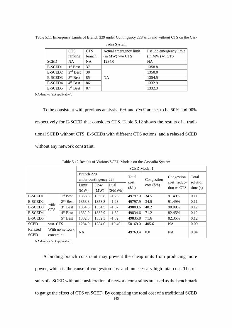
145

Table 5.11 Emergency Limits of Branch 229 under Contingency 228 with and without CTS on the Cas-

cadia System

CTS

ranking

CTS

branch

Actual emergency limit

(in MW) w/o CTS

Pseudo emergency limit

(in MW) w. CTS

SCED NA NA 1284.0 NA

E-SCED1 1st Best 37

NA

1358.8

E-SCED2 2nd Best 38 1358.8

E-SCED3 3rd Best 85 1354.5

E-SCED4 4th Best 86 1332.9

E-SCED5 5th Best 87 1332.3

NA denotes “not applicable”.

To be consistent with previous analysis, 𝑃𝑐𝑡 and 𝑃𝑐𝑡𝐶 are set to be 50% and 90%

respectively for E-SCED that considers CTS. Table 5.12 shows the results of a tradi-

tional SCED without CTS, E-SCEDs with different CTS actions, and a relaxed SCED

without any network constraint.

Table 5.12 Results of Various SCED Models on the Cascadia System

SCED Model 1

Branch 229

under contingency 228 Total

cost

($/h)

Congestion

cost ($/h)

Congestion

cost reduc-

tion w. CTS

Total

solution

time (s) Limit

(MW)

Flow

(MW)

Dual

($/MWh)

E-SCED1

with

CTS

1st Best 1358.8 1358.8 -1.23 49797.9 34.5 91.49% 0.11

E-SCED2 2nd Best 1358.8 1358.8 -1.23 49797.9 34.5 91.49% 0.11

E-SCED3 3rd Best 1354.5 1354.5 -1.37 49803.6 40.2 90.09% 0.12

E-SCED4 4th Best 1332.9 1332.9 -1.82 49834.6 71.2 82.45% 0.12

E-SCED5 5th Best 1332.3 1332.3 -1.82 49835.8 71.6 82.35% 0.12

SCED w/o. CTS 1284.0 1284.0 -10.49 50169.0 405.6 NA 0.09

Relaxed

SCED

With no network

constraint NA 49763.4 0.0 NA 0.04

NA denotes “not applicable”.

A binding branch constraint may prevent the cheap units from producing more

power, which is the cause of congestion cost and unnecessary high total cost. The re-

sults of a SCED without consideration of network constraints are used as the benchmark

to gauge the effect of CTS on SCED. By comparing the total cost of a traditional SCED

146

and the total cost of a SCED without any network constraints, the congestion cost of

the traditional SCED without CTS can be calculated and it is 405.6 $/h.

It is intuitive that the congestion cost would drop with a higher limit of the bottle-

neck branch, which is illustrated in Table 5.12. The congestion cost of E-SCED can be

reduced by 91.49% to 82.35% with the top five identified switching solutions. Fig. 5.9

presents the congestion cost associated with the traditional SCED and different E-

SCED models on the Cascadia system. With the top five identified CTS solutions being

considered in E-SCEDs respectively, the congestion cost is reduced from 405.6 $/h to

a much smaller value ranging from 34.5 $/h to 71.6 $/h.

405.6

71.6 71.2

40.2 34.5 34.5

SCED E-SCED5 E-SCED4 E-SCED3 E-SCED2 E-SCED1

0

100

200

300

400

Co

ng

esti

on

Co

st (

$/h

)

Fig. 5.9 Congestion Costs of the Traditional SCED and Various E-SCEDs on the Cascadia System.

It is interesting that the top switching action can reduce the congestion cost by

91.49% while it can only reduce the post-contingency violation by 30.78%. By imple-

menting one single switching action, the congestion cost reduction in percent for SCED

with CTS is much higher than post-contingency violation reduction in percent for

147

RTCA with CTS. One possible reason is that the marginal cost reduction with 1 MW

increase on branch limit may drop as the associated branch limit becomes higher.

Relieving the binding branch constraint by increasing the branch limit would first

allow the cheapest available unit to ramp up and force the most expensive unit to reduce

its output. After that, if that branch is still binding, further increasing the branch limit

may allow second cheapest available units to ramp up and reduce the outputs of the

second most expensive units, which would still reduce the total cost but the cost reduc-

tion for each MW relieved in the branch limit would decline.

The above conclusion can also be made from the viewpoint of flowgate pricing,

the dual variable of network constraint. With the actual emergency limit 1284.0 MW

of branch 229, the associated dual variable is -10.49 $/h, which implies that the total

cost will drop by 10.49 $/h if the emergency limit of branch 229 increase by 1 MW

from 1284.0 MW. However, when the pseudo emergency limit 1332.3 MW is used, the

associated dual variable becomes -1.82 $/h, which implies that the total cost will only

drop by 1.82 $/h if the emergency limit of branch 229 increase by 1 MW from 1332.3

MW. Thus, as the branch limit increases, the marginal total cost reduction may drop,

which implies that small post-contingency violation reduction in percent with CTS may

result in high cost reduction in percent for SCED.

Though it has been demonstrated that congestion cost can be significantly reduced

with CTS by using the pseudo emergency limits in SCED, the violation reduction per-

formance of CTS in the post-SCED stage should also be examined as the system con-

dition changes.

148

In the pre-SCED stage, the post-contingency violation reductions would be differ-

ent by implementing different switching actions and, thus, the associated pseudo limits

calculated by (5.8) would also be different in the SCED stage, which may result in

different SCED solutions. The results of traditional RTCA in the post-SCED stage, with

different CTS or pseudo limits considered in SCED, are shown in Table 5.13. The re-

sults in this table are for branch 229 under contingency 228. As expected, the post-

contingency violation increases with higher ranked beneficial switching action consid-

ered in SCED.

Table 5.13 Results of the Post-SCED RTCA with Different CTS Considered in SCED on Cascadia

CTS Actual Emergency

Rating (MVA) Flow (MVA) Violation (MVA) Over Loading

1st Best

1292.5

1376.5 84.0 6.50% 2nd Best

3rd Best 1371.6 79.0 6.11%

4th Best 1346.6 54.1 4.18%

5th Best 1345.8 53.3 4.12%

Table 5.14 shows the results of RTCA with CTS in the post-SCED stage. The

SCED solution used for Table 5.14 corresponds to the 1st best CTS solution identified

in the pre-SCED stage on the Cascadia system. The results in this table are for branch

229 under contingency 228. Before CTS, contingency 228 causes a violation of 84

MVA on branch 229 as shown in Table 5.13. However, that violation can be eliminated

with CTS. All five beneficial CTS actions identified in the pre-SCED stage are inves-

tigated in the post-SCED stage. In this case, the top two switching actions that are iden-

tified in the pre-SCED situation can reduce the post-contingency violation by about

85% while the other three switching actions can all fully eliminate the violation.

149

Table 5.14 Results of RTCA with CTS in the Post-SCED Stage with the SCED Solution Correspond-

ing to the 1st Best CTS Solution Identified in the Pre-SCED Stage on the Cascadia System

CTS Flow

(MVA)

Flow change

caused by

CTS (MVA)

Percent vio-

lation be-

yond limit

Violation

(MVA)

Violation

reduction

(MVA)

Violation

reduction in

percent

1st Best 1304.9 -71.5 0.96% 12.4 71.5 85.20%

2nd Best 1304.9 -71.5 0.96% 12.4 71.5 85.20%

3rd Best 1235.6 -140.9 0.0% -56.9 84.0 100%

4th Best 1285.8 -90.7 0.0% -6.7 84.0 100%

5th Best 1280.2 -96.3 0.0% -12.3 84.0 100%

Though the amounts of violation reduction with CTS in the post-SCED scenario

are different with the pre-SCED scenario, all CTS actions identified in the pre-SCED

scenario can reduce the flow on the overloaded branch. This demonstrates that CTS is

able to provide benefits even when the system condition has changed.

The results for considering the benefits provided by the 2nd best CTS action in

SCED would be the same with 1st best CTS action considered, since the 1st best CTS

branch and the 2nd best CTS branch are equivalent as they are in parallel and share the

same parameters.

Table 5.15, Table 5.16, and Table 5.17 show the results of RTCA with CTS in the

post-SCED stage, corresponding to different generator dispatch points obtained from

the SCEDs that considers the 3rd, 4th, and 5th best CTS solutions respectively. If the

pseudo emergency limit associated with the 3rd best CTS action is used in SCED, RTCA

simulated in the post-SCED stage results in an overload of 79 MVA on branch 229

under contingency 228; however, three of the five CTS actions can fully eliminate that

post-contingency violation while the other two CTS solutions can reduce overload by

150

more than 90%. For E-SCED with the 4th or 5th best CTS action, all five CTS actions

can fully eliminate the post-contingency overload.


ing to the 3rd Best CTS Solution Identified in the Pre-SCED Stage on the Cascadia System

CTS Flow

(MVA)

Flow change

caused by

CTS (MVA)

Percent vio-

lation be-

yond limit

Violation

(MVA)

Violation

reduction

(MVA)

Violation

reduction in

percent

1st Best 1300.0 -71.5 0.58% 7.5 71.5 90.53%

2nd Best 1300.0 -71.5 0.58% 7.5 71.5 90.53%

3rd Best 1228.5 -143.1 0.0% -64.1 79.0 100%

4th Best 1282.2 -89.3 0.0% -10.3 79.0 100%

5th Best 1277.0 -94.5 0.0% -15.5 79.0 100%


ing to the 4th best CTS Solution Identified in the Pre-SCED Stage on the Cascadia System

CTS Flow

(MVA)

Flow change

caused by

CTS (MVA)

Percent vio-

lation be-

yond limit

Violation

(MVA)

Violation

reduction

(MVA)

Violation

reduction in

percent

1st Best 1275.3 -71.3 0.0% -17.2 54.1 100%

2nd Best 1275.3 -71.3 0.0% -17.2 54.1 100%

3rd Best 1195.2 -151.4 0.0% -97.3 54.1 100%

4th Best 1263.8 -82.8 0.0% -28.7 54.1 100%

5th Best 1260.8 -85.8 0.0% -31.7 54.1 100%


ing to the 5th Best CTS Solution Identified in the Pre-SCED Stage on the Cascadia System

CTS Flow

(MVA)

Flow change

caused by

CTS (MVA)

Percent vio-

lation be-

yond limit

Violation

(MVA)

Violation

reduction

(MVA)

Violation

reduction in

percent

1st Best 1274.5 -71.4 0.0% -18 53.3 100%

2nd Best 1274.5 -71.4 0.0% -18 53.3 100%

3rd Best 1194.4 -151.5 0.0% -98.1 53.3 100%

4th Best 1263.1 -82.8 0.0% -29.4 53.3 100%

5th Best 1260.2 -85.7 0.0% -32.3 53.3 100%

With lower branch limits used for the network constraints in SCED, branches

would have more security margins in the post-SCED stage. As the congestion cost re-

duction does not vary much with different CTS solutions considered in SCED, using

151

the pseudo limit associated with the 3rd best switching actions can provide both eco-

nomic benefits and significant post-contingency violation reductions.

Market solutions of the traditional SCED and the proposed E-SCEDs are shown in

Table 5.18. When the flexibility in transmission network is taken into account, the load

payment drops significantly, as well as the generator revenue, generator rent, and con-

gestion revenue. It is observed that the amount of load payment reduction is much more

than the amount of generator rent reduction. Fig. 5.10 and Fig. 5.11 show the load pay-

ment and congestion revenue respectively, for various SCED and E-SCEDs on the Cas-

cadia system. Apparently, with higher pseudo limit used in E-SCED, the system-wide

load payment and congestion revenue substantially decreases, which implies that E-

SCED can improve the market efficiency in comparison with a traditional SCED.

Table 5.18 Market Results with SCED and Various E-SCED on the Cascadia System

Load Pay-

ment ($/h)

Generator

Revenue

($/h)

Generator

Cost ($/h)

Generator

Rent ($/h)

Congestion

Revenue

($/h)

E-SCED1 58158.48 57290.96 42839.47 14451.49 867.52

E-SCED2 58158.48 57290.96 42839.47 14451.49 867.52

E-SCED3 58112.06 57056.21 42845.19 14211.02 1055.85

E-SCED4 58977.22 57363.58 42876.2 14487.38 1613.64

E-SCED5 58977.22 57364.73 42877.34 14487.39 1612.49

SCED 74865.79 62553.62 42943.34 19610.28 12312.17

The nodal LMP including the energy component and congestion component is

shown in Table 5.19. The energy LMP of each bus is the same across the entire system

and is also equal to the LMP at the slack bus. The average LMPs and the average con-

gestion LMPs for various E-SCED are very close, since even the fifth best CTS solution

can relieve the system congestion by 82%. However, in comparison with the traditional

152

SCED, the average LMP is reduce by about 5% while the average congestion LMP is

reduced by 82% to 88%, which is consistent with the degree of congestion cost reduc-

tion as shown in Table 5.12.

74866

58977 58977 58112 58158 58158

55000

59000

63000

67000

71000

75000

Load

Pay

men

t ($

/h)

SCED

E-SCED5 E-SCED4E-SCED3 E-SCED2 E-SCED1

Fig. 5.10 Load Payment for Various SCED and E-SCEDs on the Cascadia System.

12312

1612 16141056 868 868

0

3000

6000

9000

12000

15000

Co

nges

tion

Rev

enue

($

/h) SCED

E-SCED5 E-SCED4E-SCED3 E-SCED2 E-SCED1

Fig. 5.11 Congestion Revenue for Various SCED and E-SCEDs on the Cascadia System.

153

Table 5.19 Average LMP with SCED and Various E-SCEDs on the Cascadia System

Average LMP

($/MWh)

Average Congestion LMP

($/MWh)

Energy LMP

($/MWh)

E-SCED1 7.685 0.063 7.622

E-SCED2 7.685 0.063 7.622

E-SCED3 7.649 0.071 7.578

E-SCED4 7.672 0.094 7.578

E-SCED5 7.672 0.095 7.578

SCED 8.037 0.542 7.494

5.4 Conclusions

In Chapter 4, it is demonstrated that corrective transmission switching can signifi-

cantly reduce or even fully eliminate post-contingency violations, which is believed to

reduce the need for expensive reliability-motivated generation re-dispatch and can be

translated into significant saving [147]. Thus, two procedures are proposed in this chap-

ter to investigate the potential cost saving with CTS: 1) the proposed Procedure-A rep-

resents existing industrial practice; 2) the proposed Procedure-B can fully utilize the

benefits provided by CTS in the RT SCED application. Built upon existing SCED tools,

the change required to implement the proposed Procedure-B and the proposed E-SCED

model is only to replace the actual limits with pseudo limits for branch limit constraints

in SCED, which requires minimal effort for the industry to adopt the proposed Proce-

dure-B.

Numerical simulations have demonstrated that the post-contingency violation re-

duction with CTS can translate into significant congestion cost reduction for RT SCED.

The marginal cost reduction with 1 MW increase in the limit of a bottleneck branch

may drop as the associated branch limit increases. Even with a conservative CTS solu-

tion, for instance, using the branch pseudo limit that is associated with the 3rd best CTS

154

solution in SCED, the 29% reduction in post-contingency violation is translated into

90% reduction in congestion cost in RT SCED. The case studies also demonstrate the

performance of CTS-based RTCA in the post-SCED stage. It is concluded that conges-

tion cost can be significantly reduced with the consideration of CTS.

155

6. FALSE DATA INJECTION CYBER-ATTACK DETECTION

State estimation estimates the system condition in real-time and provides a starting

point for other EMS applications including RTCA and RT SCED. Failure of state esti-

mation may cause very severe consequences. The measurements collected by state es-

timation may involve random errors, which can be identified and removed by bad data

detection. However, malicious cyber-attacks can inject false measurements that can by-

pass traditional bad data detection and result in an incorrectly estimated system condi-

tion [105]-[123]. This indicates that power system state estimation is subject to false

data injection cyber-attacks. In addition, a biased system condition may mislead oper-

ators to take unnecessary or improper actions that reduce the reliability and damage the

system. For instance, recent efforts [109]-[114] show that FDI cyber-attacks can cause

unobservable branch overloads in real-time. Thus, developing a detection approach that

can efficiently detect FDI attacks is vital for reliability enhancements and secure oper-

ations of electric power systems. The goal of FDID is to improve system reliability by

detecting FDI cyber-attacks and enhancing state estimation.

6.1 Concept

6.1.1 State Estimation

State estimation is run continuously to estimate the system status in real-time, in-

cluding bus voltages and line flows. The measurement model for state estimation can

be represented by (6.1). In (6.1), ℎ(𝑥) describes the relationship between state variable

𝑥 and measurements 𝑧, while 𝑒 denotes the measurement error vector.

𝑧 = ℎ(𝑥) + 𝑒 (6.1)

156

For DC state estimation, the relationship between state variable 𝑥 and measure-

ments 𝑧 is linear and ℎ(𝑥) can be replaced by Hx, where H is a constant Jacobian ma-

trix; then, (6.1) can be replaced by (6.2) for DC state estimation. Variable 𝑥 in (6.2)

denotes the bus voltage angle vector. This chapter focuses on the DC measurement

model, which is a linearization of (6.1).

𝑧 = 𝐻𝑥 + 𝑒 (6.2)

6.1.2 FDI Cyber-Attack

To launch an unobservable FDI cyber-attack, the injected false measurements

should meet (6.3) that represents the measurement model under attack. In (6.3), �̃� de-

notes the state variable under attack and �̃� denotes false measurements. Equation (6.4)

defines the relationship between the cyber state variable under attack and the actual

state variable; variable 𝑐 in (6.4) is referred to as the attack vector.

�̃� = 𝐻�̃� + 𝑒 (6.3)

�̃� = 𝑥 + 𝑐 (6.4)

If the attacker has access to only a part of the system, then the measurements out-

side the attack area will remain the same. Similarly, for the buses that are located out-

side the attack area, the associated elements in the attack vector 𝑐 are zeros. For sim-

plicity, it is assumed in this work that the attacker has access to the entire system.

Fig. 6.1 shows the time line that is used to illustrate FDI cyber-attacks. There are

two dispatch intervals. The assumptions made in this work are listed below:

• the attacker injects false data or measurements at 𝑡 = 0−, right before SE

and SCED execute at 𝑡 = 0,

157

• the generation at 𝑡 = −𝑇𝐸𝐷− is optimal, which implies the generation in the

first SCED period remain the same,

• system operators have accurate information at 𝑡 = −𝑇𝐸𝐷,

• the load in the second SCED dispatch interval remains constant, or the fore-

casting load at the end of the second SCED interval is the same with the

load at the beginning of the second SCED interval,

• SE executes repeatedly with the same frequency of SCED execution,

• Loads at the same bus are combined into a single aggregate load.

t = -TED

1st SCED period 2nd SCED period

t = TEDt = 0

Fig. 6.1 Time Line for Illustrating FDI Cyber-Attack

In [110], a bi-level optimization model is proposed to determine the attack vector

and false load vector that can cause the most severe loading condition on a target trans-

mission and may result in physical flow violation. Heuristics for this bi-level model are

proposed in [111]; a modified version of one of those heuristic models is presented

below,

𝑚𝑎𝑥𝑖𝑚𝑖𝑧𝑒𝑠𝑖𝑔𝑛(𝑃𝑙,0−)(𝑝𝑙 − �̃�𝑙) (6.5)

subject to

𝑝𝑘 = (𝜃𝑛(𝑘−) − 𝜃𝑛(𝑘+))/𝑋𝑘, 𝑘 ∈ 𝐾 (6.6)

�̃�𝑘 = (�̃�𝑛(𝑘−) − �̃�𝑛(𝑘+))/𝑋𝑘, 𝑘 ∈ 𝐾 (6.7)

�̃�𝑛 = 𝜃𝑛 + 𝑐𝑛, 𝑛 ∈ 𝑁 (6.8)

158

∆�̃�𝑑 = ∑ (𝑝𝑘 − �̃�𝑘)𝑘∈𝐾(𝑛(𝑑)−) − ∑ (𝑝𝑘 − �̃�𝑘)𝑘∈𝐾(𝑛(𝑑)+) , 𝑑 ∈ 𝐷 (6.9)

−𝐿𝑆𝑃𝑑 ≤ ∆�̃�𝑑 ≤ 𝐿𝑆𝑃𝑑 , 𝑑 ∈ 𝐷 (6.10)

−𝑐𝑛 ≤ 𝑠𝑛, 𝑛 ∈ 𝑁 (6.11)

𝑐𝑛 ≤ 𝑠𝑛, 𝑛 ∈ 𝑁 (6.12)

∑ 𝑠𝑛𝑛 ≤ 𝑁1 (6.13)

where 𝑃𝑙,0− denotes the actual flow on the target branch 𝑙 at 𝑡 = 0−; 𝑝𝑘 and 𝑝𝑘 denote

the expected actual flow and cyber flow on branch 𝑘 at 𝑡 = 𝑇𝐸𝐷 respectively; 𝜃𝑛 and

�̃�𝑛 denote the expected phase angle and cyber phase angle of bus n at 𝑡 = 𝑇𝐸𝐷 respec-

tively; ∆�̃�𝑑 denotes the malicious deviation of load d; and 𝐿𝑆 denotes the load shift fac-

tor.

The objective of this model is to maximize the difference between post-attack phys-

ical and cyber power flows on a pre-specified target branch l. Equations (6.6) and (6.7)

calculate the post-attack physical branch flows and cyber branch flows respectively.

Equation (6.8) shows the relationship between physical bus angles and cyber bus an-

gles. Equation (6.9) calculates the malicious load deviation vector, while (6.10) ensures

that the load shift is within the limit. The summation of the absolute change in state

variables is restricted by (6.11)-(6.13), which is equivalent to an 𝑙1-norm constraint;

where 𝑁1 is the limit of that 𝑙1-norm constraint.

The above model can be further simplified by introducing a new variable ∆𝑝𝑘 that

denotes the difference between the post-attack physical and cyber power flows. The

simplified FDI cyber-attack model is formulated below.

𝑚𝑎𝑥𝑖𝑚𝑖𝑧𝑒𝑠𝑖𝑔𝑛(𝑃𝑙,0−)∆𝑝𝑙 (6.14)

159

subject to (6.10), (6.11), (6.12), (6.13), and

∆𝑝𝑘 = (−𝑐𝑛(𝑘−) + 𝑐𝑛(𝑘+))/𝑋𝑘, 𝑘 ∈ 𝐾 (6.15)

∆�̃�𝑑 = ∑ (∆𝑝𝑘)𝑘∈𝐾(𝑛(𝑑)−) − ∑ (∆𝑝𝑘)𝑘∈𝐾(𝑛(𝑑)+) , 𝑑 ∈ 𝐷 (6.16)

where,

∆𝑝𝑙 = 𝑝𝑙 − �̃�𝑙 (6.17)

Note that this simplified 𝐵-∆𝜃 FDI cyber-attack model, consisting of (6.10)-(6.17),

is mathematically equivalent to the third heuristic algorithm presented in [111]. The

proposed 𝐵-∆𝜃 FDI cyber-attack model is implemented to provide data for the FDID

studies in this dissertation.

6.2 FDID Metrics

Two categories of metrics are proposed in this dissertation to detect potential FDI

cyber-attacks on a specific branch. They are the malicious load deviation index (MLDI)

and the branch overload risk index (BORI). MLDI can recognize load change patterns

and identify malicious load deviation, while BORI monitors suspicious changes in

branch flows. MLDI and BORI are metrics for determining whether a specific branch

is an attack target. Systematic metrics and methodology are discussed in Section 6.3.

An FDI cyber-attack alert system is also proposed in this dissertation. This system

has four different alert levels that are defined as Danger, Warning, Monitor, and Nor-

mal. The alert level can be determined by the proposed FDID metrics.

6.2.1 MLDI

As described in the previous chapter, PTDF is a matrix of sensitivity factors that

measures the incremental change in branch flow due to a change in power transferring

160

between a slack bus and a non-slack bus. Thus, given a branch, the loads that have a

significant impact on that branch should be monitored. It would be unusual if the

changes in all the loads that are critical to a branch k contribute to decreasing the flow

on branch k. Therefore, based on this observation, a malicious load deviation index is

proposed to detect potential FDI cyber-attacks. Given a branch k, 𝑀𝐿𝐷𝐼𝑘 can be calcu-

lated by (6.18),

𝑀𝐿𝐷𝐼𝑘 = 𝑠𝑖𝑔𝑛(𝑃𝑘−)∑ 𝐼𝑛𝑑𝑐𝑡𝑟𝑑,𝑘𝑑∈𝐷(𝑘)

𝑁𝐷𝑘 (6.18)

where

𝐼𝑛𝑑𝑖𝑐𝑡𝑟𝑑,𝑘 =

{

−𝑠𝑖𝑔𝑛(𝑃𝑇𝐷𝐹𝑛(𝑑),𝑘),𝑖𝑓

𝑃𝑑0,𝐼𝑆𝑂−𝑃𝑑−

𝑃𝑑−≤ −5%

0,𝑖𝑓 − 5% <𝑃𝑑0,𝐼𝑆𝑂−𝑃𝑑−

𝑃𝑑−< 5%

𝑠𝑖𝑔𝑛(𝑃𝑇𝐷𝐹𝑛(𝑑),𝑘),𝑖𝑓𝑃𝑑0,𝐼𝑆𝑂−𝑃𝑑−

𝑃𝑑−≥ 5%

(6.19)

and,

𝑁𝐷𝑘 = ∑ 1𝑑∈𝐷(𝑘) (6.20)

where D(k) denotes a set of loads that are critical to branch k. If the absolute value of

𝑃𝑇𝐷𝐹𝑛(𝑑),𝑘 is not less than 1%, then, load d is defined to be critical to branch k.

Though 𝑀𝐿𝐷𝐼𝑘 is in the range of [-1, 1] theoretically, 𝑀𝐿𝐷𝐼𝑘 is typically close to

zero if the load fluctuates randomly. A positive value indicates that the load change

might reduce the flow on branch k. A very high positive value may imply the load

fluctuation is abnormal and the probably of branch k being targeted by an FDI attack is

high.

Metric 𝑀𝐿𝐷𝐼𝑘 only considers the number of load buses that are critical to a branch,

but fails to take load magnitude and PTDF values into account. To consider those two

161

factors, an enhanced malicious load deviation index (EMLDI) is proposed in this work.

Similar to 𝑀𝐿𝐷𝐼𝑘, 𝐸𝑀𝐿𝐷𝐼𝑘 is defined by (6.21),

𝐸𝑀𝐿𝐷𝐼𝑘 = 𝑠𝑖𝑔𝑛(𝑃𝑘−)∑ (𝐼𝑓𝑑,𝑘𝐼𝑛𝑑𝑖𝑐𝑡𝑟𝑑,𝑘)𝑑∈𝐷(𝑘) (6.21)

where,

𝐼𝑓𝑑,𝑘 =|(𝑃𝑑0,𝐼𝑆𝑂−𝑃𝑑−)∙𝑃𝑇𝐷𝐹𝑛(𝑑),𝑘|

∑ |(𝑃𝑑0,𝐼𝑆𝑂−𝑃𝑑−)∙𝑃𝑇𝐷𝐹𝑛(𝑑),𝑘|𝑑∈𝐷(𝑘) (6.22)

𝐸𝑀𝐿𝐷𝐼𝑘 shares the same range and indication with 𝑀𝐿𝐷𝐼𝑘. The difference is that

the effects of load magnitude and PTDF values are not considered for 𝑀𝐿𝐷𝐼𝑘 but are

captured by 𝐸𝑀𝐿𝐷𝐼𝑘. Thus, given a potential target branch k, 𝐸𝑀𝐿𝐷𝐼𝑘 may be a better

indicator to determine whether there is an attack targeting that branch.

The alert level criteria for 𝑀𝐿𝐷𝐼𝑘 and 𝐸𝑀𝐿𝐷𝐼𝑘 are the same and defined in Table

6.1. With the proposed metrics and alert system, it is not very hard to identify whether

a specified branch is under attack. As 𝐸𝑀𝐿𝐷𝐼𝑘 considers more factors than 𝑀𝐿𝐷𝐼𝑘, the

alert level for branch k should be determined by 𝐸𝑀𝐿𝐷𝐼𝑘. In this work, 𝐴𝐿𝑀𝑘 denotes

the alert level associated with 𝑀𝐿𝐷𝐼𝑘 while 𝐴𝐿𝐸𝑘 denotes the alert level associated

with 𝐸𝑀𝐿𝐷𝐼𝑘.

Table 6.1 Alert Level Criteria based on 𝑀𝐿𝐷𝐼𝑘 or 𝐸𝑀𝐿𝐷𝐼𝑘

Alert level 𝑀𝐿𝐷𝐼𝑘 or 𝐸𝑀𝐿𝐷𝐼𝑘

Danger >50%

Warning >35%

Monitor >20%

Normal <20%

6.2.2 BORI

The first category of FDID metrics monitors load change and identifies potential

attacks while the second category of FDID metrics monitors flow changes and identifies

162

potential overloads. As introduced above, in order to execute an unobservable FDI

cyber-attack that would overload a line, the attacker needs to change the measurements

including load measurements that are sent to the system operators. In the cyber world,

the attacker can deliberately reduce the flow on a congested line or a heavily loaded

line by shifting loads. This would mislead operators to believe that there is extra avail-

able capacity on the target branch; then, operators may re-dispatch generation to take

advantage of that extra available capacity and reduce the total cost. However, in the real

world, there is no such extra available capacity and physical overloads may occur. Thus,

based on this type of flow change pattern, this work proposes a branch overload risk

index to detect FDI cyber-attacks.

Considering the attacker may or may not take the effect of generation re-dispatch

into account, two similar but different metrics, BORI1 and BORI2, are proposed in this

dissertation. BORI1 only considers the flow changes during the previous interval while

BORI2 takes the SCED results into account. BORI1 and BORI2 are defined in (6.23)

and (6.24) respectively.

𝐵𝑂𝑅𝐼1𝑘 = 𝑠𝑖𝑔𝑛(𝑃𝑘−)(𝑃𝑘− − 𝑃𝑘0,𝐼𝑆𝑂 + 𝑃𝑘−)/𝐿𝑖𝑚𝑖𝑡𝐴𝑘 (6.23)

𝐵𝑂𝑅𝐼2𝑘 = 𝑠𝑖𝑔𝑛(𝑃𝑘−)(𝑃𝑘− − 𝑃𝑘0,𝐼𝑆𝑂 + 𝑃𝑘+,𝑆𝐶𝐸𝐷)/𝐿𝑖𝑚𝑖𝑡𝐴𝑘 (6.24)

A comprehensive metric 𝐵𝑂𝑅𝐼𝑘 is proposed to combine those two metrics belong-

ing to the second category of FDID metrics. As shown in (6.25), 𝐵𝑂𝑅𝐼𝑘 is defined to

be the larger between 𝐵𝑂𝑅𝐼1𝑘 and 𝐵𝑂𝑅𝐼2𝑘.

𝐵𝑂𝑅𝐼𝑘 = 𝑚𝑎𝑥(𝐵𝑂𝑅𝐼1𝑘, 𝐵𝑂𝑅𝐼2𝑘) (6.25)

163

The alert level criterion for 𝐵𝑂𝑅𝐼𝑘 is defined in Table 6.2. In this work, 𝐴𝐿𝐵𝑘 de-

notes the alert level associated with 𝐵𝑂𝑅𝐼𝑘. 𝐵𝑂𝑅𝐼𝑘 and 𝐴𝐿𝐵𝑘 enable operators to de-

termine whether a branch is under attack from the viewpoint of flow violations.

Table 6.2 Alert Level Criteria based on 𝐵𝑂𝑅𝐼𝑘

Alert level 𝐵𝑂𝑅𝐼𝑘

Danger >115%

Warning >110%

Monitor >105%

Normal <105%

6.3 Two-stage FDID Approach

Metrics MLDI and BORI presented in Section 6.2 are used to detect potential FDI

attacks on a specific branch rather than monitor the system as a whole. Thus, a system-

atic approach is desired. In this section, a two-stage FDID approach, consisting the FDI

attack awareness stage and the target branch identification stage, is proposed to detect

potential FDI cyber-attacks. The first stage is to determine whether the system is under

FDI cyber-attack and the second stage would identify the target branch.

6.3.1 Stage 1: FDI Attack Awareness

As introduced in Section 6.2, MLDI and BORI are proposed to detect whether an

FDI cyber-attack is launched for a specific branch. Since system operators have limited

information regarding which branch the attacker would target, it is necessary to calcu-

late the metrics for all branches. However, given that a practical power system typically

has a large number of branches, even random load fluctuations may cause large 𝑀𝐿𝐷𝐼𝑘,

𝐸𝑀𝐿𝐷𝐼𝑘, and 𝐵𝑂𝑅𝐼𝑘 values for a few branches, which may mislead system operators

164

to believe that the load fluctuation is abnormal and the system is under attack. There-

fore, a system-wide malicious load deviation index (SMLDI) is proposed to resolve this

issue. SMLDI is defined in the equation shown below,

𝑆𝑀𝐿𝐷𝐼 =∑ 𝑀𝐿𝐷𝐼𝑘𝑘∈𝐾𝐴

∑ 1𝑘∈𝐾𝐴 (6.26)

where KA is a set of ten branches that have the top ten 𝑀𝐿𝐷𝐼𝑘 values. If the number of

load buses that have significant effects on branch k is too small, then the associated

𝑀𝐿𝐷𝐼𝑘 cannot be used for malicious load deviation recognition and branch k will not

be included in the set KA. In this work, branches that have less than five critical load

buses will not be considered as a candidate element of set KA.

In this stage, SMLDI is used as the only metric to determine whether the system is

under attack. Similar to the alert level designed for a target line, a system-wide FDI

alert level is defined in Table 6.3. A system would be considered to be FDI cyber-attack

free if the associated alert level is marked as Normal or Monitor in stage 1. Only the

cases that have either Warning or Danger alert flags will be sent to stage 2 for FDI

target branch identification.

Table 6.3 Alert Level Criteria based on 𝑆𝑀𝐿𝐷𝐼

Alert level 𝑆𝑀𝐿𝐷𝐼

Danger >50%

Warning >35%

Monitor >20%

Normal <20%

6.3.2 Stage 2: Target Branch Identification

It is vital to determine whether the system is under malicious FDI cyber-attack in

stage 1. It is also very important to identify which branch is the attacker’s target so that

165

system operators can take immediate actions to handle the detected FDI attack. Thus,

the goal of stage 2 is to identify the target branch.

As presented above, 𝐸𝑀𝐿𝐷𝐼𝑘 detects FDI attacks targeting branch k from the view-

point of suspicious load deviation while 𝐵𝑂𝑅𝐼𝑘 detects FDI attacks targeting branch k

from the viewpoint of potential flow violation. Both of the metrics are considered in

this stage. The alert levels associated with 𝐸𝑀𝐿𝐷𝐼𝑘 and 𝐵𝑂𝑅𝐼𝑘 can be combined into a

single comprehensive FDI attack alert level. The combination of the two alert levels is

defined in Table 6.4. This comprehensive alert level, denoted by 𝐴𝐿𝐶𝑘, is used as the

alert level for identifying the target branch.

Table 6.4 Comprehensive Alert Level Combined from Two Separate Alert Levels

Alert level Alert level

Normal Monitor Warning Danger

Normal Normal Monitor Monitor Warning

Monitor Monitor Monitor Warning Warning

Warning Monitor Warning Warning Danger

Danger Warning Warning Danger Danger

Though the proposed alert system can provide a qualitative analysis, it is also very

important to analyze the FDI attack quantitatively. Thus, a comprehensive FDI attack

index (CI) that considers both load deviation patterns and potential branch overloads is

proposed in this work. 𝐶𝐼𝑘 is defined in (6.27). Thus, the branch that has the biggest

𝐶𝐼𝑘 is considered to be the most suspicious target branch; moreover, the 𝐶𝐼𝑘 rank can

serve as a metric that indicates the possibility of branch k being the target branch.

𝐶𝐼𝑘 =𝐸𝑀𝐿𝐷𝐼𝑘 𝐵𝑂𝑅𝐼𝑘 (6.27)

Therefore, the proposed comprehensive index 𝐶𝐼𝑘 and the proposed comprehen-

sive alert level 𝐴𝐿𝐶𝑘 are used to identify the target branch in stage 2. In this work, the

166

branches that are marked as Danger or have a 𝐶𝐼𝑘 ranking in the top three are consid-

ered to be the most suspicious target branches.

6.4 Case Studies

The IEEE 118-bus test system is used in this work to investigate the proposed 𝐵-

∆𝜃 FDI cyber-attack model presented in Section 6.1.2. Then, this test case is further

used to examine the proposed two-stage FDID approach, as well as the proposed FDI

cyber-attack alert system. This case contains 118 buses, 186 branches, and 19 online

units. The initial total load at 𝑡 = −𝑇𝐸𝐷 is 4,242 MW. Out of 118 buses, 99 buses are

load buses or have non-zero loads.

6.4.1 FDI Results

In this section, to study the effectiveness of the proposed 𝐵-∆𝜃 FDI cyber-attack

model, numerical simulations are conducted with different system scenarios including

constant load scenarios and random load fluctuation scenarios in the first dispatch in-

terval, from 𝑡 = −𝑇𝐸𝐷 to 𝑡 = 0. The effects of different load shift factors and 𝑙1-norm

constraint limits on the physical consequences of an FDI attack are also analyzed in this

section.

By assuming the load profile does not change in the first dispatch interval, the max-

imum power flows on branch 111 and branch 118 with different FDI attack settings are

presented in Fig. 6.2 and Fig. 6.3 respectively. The blue curve with diamond markers

in Fig. 6.2 corresponds to the FDI results with a load shift factor of 5% and it becomes

flat quickly. The reason is that the load shift constraint is binding when 𝑁1 is 6 and

further relaxing the 𝑙1-norm constraint will not change the FDI results.

167

Fig. 6.2 Maximum Power Flow on Line 111 with Various Load Shift Factors and 𝑙1-Norm Constraint

Limits.

Fig. 6.3 Maximum Power Flow on Line 118 with Various Load Shift Factors and 𝑙1-Norm Constraint

Limits.

168

Since the 𝐵-∆𝜃 FDI model proposed in this work is a fast heuristic rather than an

exact approach, the maximum flows shown in Fig. 6.2 and Fig. 6.3 do not strictly in-

crease as the load shift factor or 𝑙1-norm constraint limit increases. However, with a

more flexible condition, the attacker can typically cause more severe flow violations.

In reality, loads fluctuate all the time. Thus, it is important to analyze the effects of

random load fluctuations on FDI cyber-attacks. It is assumed that the load fluctuation

follows the normal distribution with a mean of 𝜇 (a percentage) and a standard devia-

tion 𝜎 (a percentage), which is denoted by N(𝜇, 𝜎). The process of generating a load

fluctuation vector following N(𝜇, 𝜎) is presented below:

1) generate a vector 𝑣 that follows standard normal distribution,

2) apply a cutoff value 1.96 to this vector 𝑣,

3) adjust 𝑣 with equation: 𝑣 = 𝑣𝜎 + 𝜇,

4) create a load fluctuation vector: ∆𝑝𝑑 = 𝑃𝑑−𝑣.

Note that since loads do not fluctuate significantly in the short-term, step 2) ensures

that the random load fluctuation does not have a long tail distribution.

For the FDI simulations conducted in this section, the random load fluctuation fol-

lows N(0, 3%). For each FDI attack simulated, the load profile is updated with a differ-

ent randomly generated load fluctuation vector. The results of FDI attacks with load

fluctuations are presented in Fig. 6.4 and Fig. 6.5. Fig. 6.4 shows the results of an FDI

attack targeting branch 111 while Fig. 6.5 shows the results of an FDI attack targeting

branch 118. The curves in Fig. 6.4 and Fig. 6.5 look very similar to the corresponding

curves in Fig. 6.2 and Fig. 6.3 respectively. Random load fluctuations may either relieve

169

the violation or contribute to the violation to a limited extent. Fig. 6.4 and Fig. 6.5 show

that an FDI cyber-attack can still result in a flow violation on the target branch even

with random load fluctuations.

Fig. 6.4 Maximum Power Flow on Line 111 with Random Load Fluctuation.

Fig. 6.5 Maximum Power Flow on Line 118 with Random Load Fluctuation.

170

6.4.2 FDID Results

Stage 1: FDI Attack Awareness

As introduced above, the proposed FDID strategy consists of two stages. Stage 1

determines whether the system is under an FDI cyber-attack by analyzing the load pro-

file changes. It is important to detect FDI attacks. Furthermore, it is also vital to bypass

random load fluctuations. The goal of stage 1 is to have a low false alarm probability

as well as a low false dismissal probability.

Two sets of load deviation vectors, including the FDI malicious load deviation vec-

tors and random load fluctuation vectors, are tested in this stage. The load deviation

vector denotes the difference between the loads at the beginning of the second dispatch

interval (𝑡 = 0) and the loads profile at the beginning of the first dispatch interval (𝑡 =

−𝑇𝐸𝐷). The first set of malicious load deviation vectors can be obtained from the 160

different FDI attacks performed in Section 6.4.1. The second set of normal load fluctu-

ation vectors is created with four different normal distributions: N(0, 3%), N(0, 5%),

N(-1%, 3%), and N(1%, 3%). Twenty independent vectors are generated for each nor-

mal distribution. Thus, the second set has a total of 80 normal load fluctuation vectors.

The SMLDI values for those 240 load change vectors are calculated in stage 1. The

results for the 160 FDI malicious load deviation vectors and 80 random load fluctuation

vectors are presented in Table 6.5 and Table 6.6 respectively. The SMLDI values for

the random load fluctuation vectors are very small and the averages are close to zero.

As for the FDI malicious load deviation vectors, the associated SMLDI values are much

bigger and the average values are around 70%. This indicates that FDI cyber-attacks

171

can be successfully detected with the proposed metric SMLDI and random load fluctu-

ations can successfully bypass this two-stage FDID approach.

Fig. 6.6 shows a scatter plot of the SMLDI values for all the random load fluctua-

tions and FDI cyber-attacks simulated in this work. The blue squares correspond to the

random load fluctuation vectors while the red triangles correspond to the FDI malicious

load deviation vectors. As shown in Fig. 6.6, the SMLDI values for the random load

fluctuation vectors are all below 35% and, thus, the associated alert levels are either

Normal or Monitor. The alert levels for most random vectors are Normal. As for the

FDI malicious load deviation vectors, the associated SMLDI values are all above the

warning tolerance and the alert levels for most FDI attack load deviation vectors are

Danger. Therefore, it is demonstrated that the proposed metric SMLDI can efficiently

detect FDI cyber-attacks and would not mistakenly identify a random load fluctuation

as an FDI attack. In other words, the results presented in Fig. 6.6 demonstrate the pro-

posed two-stage FDID approach has a very low false alarm rate as well as a very low

false dismissal rate.

The first 80 system scenarios in Fig. 6.6 correspond to random load fluctuations

with four different normal distributions. They are listed as the order of N(0, 3%), N(0,

5%), N(-1%, 3%), and N(1%, 3%). Each normal distribution has 20 scenarios. By com-

paring the random load fluctuations generated with different normal distribution func-

tions, it is observed that the mean of load fluctuation does not affect the metric while

higher standard deviations may result in higher SMLDI values. This is consistent with

172

the statistics presented in Table 6.6. This implies that the false alarm rate for the pro-

posed approach may increase as the magnitude of load deviation increases. It is worth

noting that loads typically do not deviate too much in a short time frame.

Fig. 6.7 illustrates the SMLDI values that are associated with various FDI attacks

targeting branch 118 with random load fluctuations that follow N(0, 3%) in the first

dispatch interval. The red dotted line is the boundary between the alert levels Monitor

and Warning. Those SMLDI values are well above the Warning alert tolerance of 35%,

especially for the cases that have more flexible constraints. It is very straightforward

and efficient to identify whether the system is under malicious FDI cyber-attack with

the proposed metric SMLDI.

Table 6.5 SMLDI Values for FDI Malicious Load Deviation Vectors

Attack on branch 118 Attack on branch 111

Constant load N(0, 3%) Constant load N(0, 3%)

max 97.8% 97.8% 97.8% 97.5%

min 48.8% 39.9% 35.7% 38.7%

median 62.9% 68.5% 62.9% 63.8%

average 72.1% 74.5% 68.6% 70.7%

std 16.8% 19.0% 19.4% 20.3%

Table 6.6 SMLDI Values for Random Load Fluctuation Vector

Normal load fluctuation only

N(0, 3%) N(0, 5%) N(-1%, 3%) N(1%, 3%)

max 23.1% 28.0% 23.5% 20.9%

min 3.2% 13.8% 5.5% 7.5%

median 11.8% 22.8% 12.0% 12.5%

average 12.2% 21.7% 12.4% 13.2%

std 4.4% 3.7% 4.7% 3.7%

173

SM

LD

I

Random vector FDI attack vector

Normal

Monitor

Warning

Danger

Fig. 6.6 SMLDI Values for Random Load Fluctuations and FDI Cyber-Attacks.

Fig. 6.7 SMLDI of FDI Attacks for Target Branch 118 with N(0, 3%) Random Load Fluctuation.

Stage 2: Target Branch Identification

In this stage, only the cases that are identified to be under FDI cyber-attack will be

examined. Thus, only those 160 FDI attack scenarios are sent to the target branch iden-

tification routine.

Table 6.7 shows the results of target line identification for FDI attacks on branch

111 with a load shift factor of 10% and no random load fluctuations in the first dispatch

174

interval. Out of the ten system scenarios, the metric 𝐶𝐼𝑘 of branch 111 ranks first for

the nine scenarios and ranks second for the remaining one scenario. There are eight

scenarios for which branches marked as Danger exist; branch 111 is the only one that

is marked as Danger for those eight scenarios. Therefore, both the proposed compre-

hensive FDID index and the proposed comprehensive alert level indicate that branch

111 is the most suspicious target branch. Table 6.8 shows the results of target line iden-

tification for FDI attacks on branch 111 with a load shift factor of 10% and a random

load fluctuation that follows N(0, 3%). The difference between the two sets of simula-

tions associated with Table 6.7 and Table 6.8 respectively is that the simulations corre-

sponding to Table 6.7 do not involve random load fluctuations. Therefore, the results

shown in Table 6.8 are more realistic. However, the conclusions drawn from Table 6.8

are similar to Table 6.7. This indicates that the proposed method is effective even when

the normal load fluctuation is modeled.

Table 6.7 Target Line Identification Results for FDI Attacks on Line 111 with a Load Shift Factor of

10% and No Random Load Fluctuation in the First Dispatch Interval

𝐶𝐼111 Rank of

𝐶𝐼111 𝐴𝐿𝐶111 𝐴𝐿𝐸111 𝐴𝐿𝐵111

Number of lines

marked Danger

List of suspi-

cious target lines

N1 = 1 0.46 2 Monitor Warning Normal 0 145, 111, 150

N1 = 2 0.66 1 Warning Danger Monitor 0 111, 129, 145

N1 = 3 0.90 1 Danger Danger Warning 1 111, 129, 181

N1 = 4 1.13 1 Danger Danger Danger 1 111, 119, 141







175

Table 6.9 presents the FDID results on various FDI attacks. As shown in Table 6.9,

the target branches are correctly identified for 96.9% or 155 scenarios out of the 160

FDI cyber-attacks. The target branch is marked as Danger for over 90% of the FDI

attacks on branch 118. The percentage of the cases that the target line for the FDI attacks

on line 111 is marked as Danger is relatively low. The reason is that the overloads on

line 111 for some attacks, including most FDI attacks with a load shift factor of 5%, are

not very significant and do not reach the Warning alert threshold. However, the associ-

ated comprehensive FDI attack index 𝐶𝐼 of line 111 ranks first for most cases. For all

FDID tests on the 160 FDI attacks, the FDID comprehensive index 𝐶𝐼 of the target line

ranks very high and almost all of the FDID comprehensive indices rank either first or

second.

Table 6.8 Target Line Identification Results for FDI Attacks on Line 111 with a Load Shift Factor of

10% and N(0, 3%) Load Random Fluctuation in the First Dispatch Interval

𝐶𝐼111 Rank of

𝐶𝐼111 𝐴𝐿𝐶111 𝐴𝐿𝐸111 𝐴𝐿𝐵111

Number of lines

marked Danger

List of suspi-

cious target lines

N1 = 1 0.45 2 Monitor Warning Normal 0 145, 111, 150

N1 = 2 0.68 1 Warning Danger Monitor 0 111, 129, 145









176

Table 6.9 Results of FDID on Various FDI Attacks

Attack on line 118 Attack on line 111

Total Constant

load N(0, 3%)

Constant

load N(0, 3%)

Average 𝐶𝐼𝑘 rank of the target line 1.58 1.55 1.13 1.33 1.39

Percent of scenarios for which the

target line is identified 92.5% 100% 100% 95.0% 96.9%

Percent of scenarios for which the

target line is marked as Danger 92.5% 92.5% 65% 77.5% 81.9%

Number of scenarios simulated 40 40 40 40 160

6.5 Conclusions

Recent work in the literature has demonstrated that power systems are subject to

unobservable FDI cyber-attacks in real-time. Attackers can cause flow violations that

are neither observed nor detected by conventional state estimation. Therefore, it is very

important to develop a strategy that can quickly detect such malicious FDI cyber-at-

tacks in real-time.

An FDI model is first proposed in this dissertation in order to examine the effects

of FDI attacks on system reliability. Then, a two-stage strategy is proposed to detect

FDI attacks. Two categories of metrics, MLDI and BORI, are proposed and used in this

two-stage approach to determine whether the change in system condition is abnormal.

MLDI recognizes malicious load changes while BORI identifies suspicious flow

changes. In stage 1, the proposed system-wide MLDI is used to determine whether the

system is under attack. If the system is deemed to be under attack, stage 2 will launch

and the proposed alert system and comprehensive FDID index will be used to identify

the attack target branch.

Simulation results show that FDI cyber-attacks can cause physical flow violations

and, then, demonstrates the effectiveness of the proposed FDID metrics, FDI cyber-

177

attack alert system, and two-stage FDID approach. The proposed two-stage FDID ap-

proach successfully detects all 160 FDI attacks that are simulated in this work and cor-

rectly identifies the target branch for about 97% of the cases. In addition, random load

fluctuations will not activate the FDID alert system. Numerical simulations conducted

on 80 different random load fluctuation vectors show that none of the random load

fluctuation scenarios are mistakenly identified as malicious load deviations. To con-

clude, normal load fluctuations will not activate the proposed FDI alert system, while

the proposed two-stage FDID approach can efficiently detect FDI attacks and the target

branch. In other words, the false alarm rate and false dismissal rate for the proposed

two-stage FDID approach are very low.

178

7. CONCLUSIONS

Transmission components are traditionally modeled as static assets in power sys-

tem real-time operations. Although previous studies have demonstrated transmission

switching can provide a variety of benefits, they are based on a DC framework and are

verified with small test systems. Directly modeling transmission switching in RTCA

and RT SCED will cause a serious computational burden and substantially increase the

solution time, which is impractical for real-time applications. Therefore, this disserta-

tion proposes CTS to utilize the flexibility in transmission networks in a practical way.

The reliability benefits and economic benefits provided by CTS are investigated on

large-scale power systems on an AC framework. The proposed CTS can reduce post-

contingency violations as an inexpensive corrective strategy and reduce congestion cost

by relieving critical network constraints.

If an unexpected critical contingency is not handled properly, it may result in a

serious emergency and cause blackouts. RTCA identifies critical contingencies and the

associated violations. With RTCA, pre-planned strategies can be made in advance to

deal with potential critical contingencies. One widely used strategy is to re-dispatch

generation to eliminate potential post-contingency violations. However, reliability-mo-

tivated generation re-dispatch is typically very expensive.

In this dissertation, CTS is proposed as another technique to handle potential post-

contingency violations. Over 1.5 million contingencies are simulated on three large-

scale practical power systems (TVA, ERCOT, and PJM) to evaluate the effectiveness

of CTS with respect to post-contingency violation reduction. Numerical simulations

179

using the full AC power flow model show that each system is subject to critical contin-

gencies and the proposed CTS algorithms can effectively reduce potential post-contin-

gency violations. For instance, the average flow violation reduction achieved with CTS

is around 60% for the PJM system. The percent of contingencies for which the associ-

ated violations can be fully eliminated by CTS is greater than 25% while the percent of

contingencies where there is no beneficial CTS solution is less than 10%.

It is verified that CTS can provide operators with an alternative corrective strategy

to relieve both flow violations and voltage violations caused by critical contingencies.

Multiple beneficial switching actions are available, which provide operators with

choices. Substantial post-contingency violation reduction can be achieved with the pro-

posed heuristic algorithms that can achieve very similar results with complete enumer-

ation but are much faster. Parallel computing can further reduce the solution time. Pa-

reto improvement is proposed to investigate the impact of CTS on individual element.

The benefits achieved with and without enforcing Pareto improvement are very similar;

in other words, most identified CTS solutions can reduce post-contingency violations

at an aggregate level while creating no additional violations on any individual element.

Incorporating CTS in RTCA can substantially improve system reliability. In exist-

ing EMS, RTCA provides RT SCED with a list of network constraints. As CTS can

efficiently reduce or even eliminate post-contingency violations, the network con-

straints sent to RT SCED can be relaxed, which reduce the need for reliability-moti-

vated generation re-dispatch. Simulation results on the Cascadia system illustrate sig-

nificant (about 90%) cost reduction can be achieved when modeling CTS in RT SCED.

180

Two procedures are proposed in this dissertation to connect RTCA and RT SCED.

Procedure-A represents the traditional procedure used in industry. In Procedure-A, the

potential post-contingency violations are sent to RT SCED, as well as the actual base-

case violations. RT SCED determines the optimal dispatch solution that has the least

cost while all violations are eliminated and reliability requirements are met. Although

the solution provided by RT SCED is on a DC model basis, it is fully evaluated on an

AC framework and the effectiveness of Procedure-A is demonstrated. Multiple SCED

models with different forms of network constraints are investigated and the hot-start

PTDF model based SCED is shown to have the best performance.

Procedure-B, an enhanced version of Procedure-A, is proposed to integrate CTS

into existing real-time operational modules in EMS. Procedure-B can capture the reli-

ability benefits of CTS in RT SCED. With the proposed concept of pseudo limit, the

transition from Procedure-A to more advanced Procedure-B requires minimal change,

which is the replacement of actual limits with pseudo limits for the contingency-case

network constraints in RT SCED. Numerical simulations show that substantial conges-

tion cost reduction can be achieved by considering CTS in RT SCED; The beneficial

CTS actions identified in the pre-SCED stage can also reduce the violations caused by

the same contingency in the post-SCED stage even if the system condition may have

changed significantly.

Full utilization of the network flexibility could benefit power systems significantly.

Transmission switching has gained ISOs’ considerable attention in various areas in

power systems since CTS can add flexibility in power system real-time operations. The

181

cost to implement CTS is low since the required hardware is already available in the

field of existing power systems. In this dissertation, it is demonstrated that CTS is able

to provide reliability benefits in regard to post-contingency violation reduction as well

as economic benefits with respect to congestion cost reduction. Moreover, the proposed

mechanism of integrating CTS into EMS including RTCA and RT SCED will require

minimal change; in other words, CTS can be considered as an add-on module for exist-

ing EMS. Thus, with the proposed mechanism, it is not very difficult for the industry

to adopt CTS for real-time operations.

The traditional bad data detection function of state estimation can effectively iden-

tify large measurement errors and outliers that would dramatically drift the estimated

system status away from the actual system status. It ensures the impact of random meas-

urement noises on state estimation is minimal. However, malicious FDI cyber-attacks

can inject false measurements that are designed to meet the physical laws and bypass

bad data detection. Thus, state estimation under FDI attack would provide an inaccurate

base case for other EMS applications. This would mislead system operators to adjust

the generation improperly, which may cause unobservable flow violations. Numerical

simulations show that FDI cyber-attacks can cause severe flow violations in real-time.

Therefore, it is very important to identify FDI cyber-attack effectively.

Several metrics are proposed to monitor abnormal load deviations and flow

changes. An FDI cyber-attack alert system is proposed to identify FDI attacks. It is very

unlikely that a system is under FDI attack if the corresponding alert level is marked as

Normal or Monitor. However, the system can be considered to be under FDI attack

182

when the alert flag is marked as Warning or Danger. Based on the proposed metrics

and alert system, a systematic two-stage FDID approach is proposed to detect malicious

FDI cyber-attacks. The first stage determines whether a system is under attack. For the

cases that are deemed to be under attack, they will be sent to the target branch identifi-

cation routine in the second stage. Case studies demonstrate the effectiveness of the

proposed two-stage FDID approach. The proposed approach successfully detects all

160 FDI attacks and identifies the target correctly for about 97% of the cases. The false

alarm rate is zero as none of the normal load fluctuations activate the proposed alert

system.

In conclusion, this dissertation proposes a two-stage FDID approach that can ef-

fectively detect FDI cyber-attacks and secure state estimation. After state estimation

determines the system status in real-time, RTCA would execute and identify the poten-

tial network violations that would be converted into network constraints for RT SCED.

Traditional RTCA and RT SCED treat the transmission network as a static network and

are not able to capture the flexibility in the transmission network. In this dissertation,

corrective transmission switching is proposed to enable operators to utilize the flexibil-

ity in the transmission network. Incorporating CTS into RTCA and RT SCED can en-

hance system reliability and reduce the total cost. The proposed approaches are demon-

strated with the cases that are tested in this dissertation, while it is worth noting that

they can be applied to other systems as well.

183

8. FUTURE WORK

The effects of CTS on RTCA and RT SCED are examined in this dissertation.

Heuristics are proposed to create the ranked switching list and identify the beneficial

switching solutions in real-time. Case studies show that CTS can efficiently reduce

post-contingency violations. With the reliability benefits provided by CTS, higher lim-

its are available for contingency-case network constraints in RT SCED, which substan-

tially reduce congestion cost.

The reliability benefits of employing CTS in RTCA are tested on the TVA, ER-

COT, and PJM systems. Numerical simulations verify the effectiveness of CTS. The

results are promising and convincing as the test cases are large-scale practical power

systems with real EMS data. The proposed heuristics that can quickly identify benefi-

cial switching solutions include two vicinity-based local search algorithms (CBCE and

CBVE) and two different data mining methods (RDM and EDM). In addition, sensitiv-

ity factors, mainly LODF, may be a good indicator to identify the beneficial CTS solu-

tions for flow violation reduction. Thus, potential future work is to investigate LODF

based heuristic algorithm for identifying the candidate CTS list. Since NERC requires

power systems to be N-1 reliable, another potential future work is to ensure the system

is N-1 reliable in the post-switching situation.

With the availability of CTS as a corrective control scheme, higher short-term

branch limits can be used in RT SCED, which reduces congestion cost significantly.

Numerical simulations on the Cascadia system demonstrate the effectiveness of CTS in

terms of congestion cost reduction. Though RT SCED is based on DC power flow

184

model, AC feasibility of the RT SCED solutions is verified by performing AC power

flow, AC contingency analysis, and AC transmission switching simulations in the post-

SCED stage. This work is tested on the Cascadia system, which is an artificial 179-bus

system. Therefore, in order to demonstrate the robustness and effectiveness of the pro-

posed strategy for integrating CTS into RT SCED, potential future work is to investi-

gate this strategy on large-scale realistic power systems.

False data injection cyber-attacks can compromise measurements that are sent to

the control center and result in biased state estimation solutions. This could further mis-

lead operators to take improper adjustments and cause physical flow violations, which

would jeopardize system security. Thus, it is key to detecting FDI cyber-attacks effi-

ciently. This dissertation implements an FDI heuristic method to show the physical

consequences of an FDI attack and proposes a two-stage FDID approach to identify

potential FDI attacks. Case studies demonstrate that FDI attack can overload the target

branch and that the proposed FDID approach can efficiently detect FDI attacks. It is

worth noting that: 1) the simplified DC model is used rather than the full AC model; 2)

it is assumed that attackers have access to the entire system; and 3) the test case is the

IEEE 118-bus system that is small-scale and artificial. Therefore, future work may ex-

tend this work to AC framework with a more realistic assumption that attackers have

limited access to only a single area rather than access to the entire system; numerical

simulations on large-scale practical power systems are also desired.

185

REFERENCES

[1]. U.S. Department of Energy, “Large Power Transformers and the U.S. Electric

Grid - Infrastructure Security and Energy Restoration Office of Electricity De-

livery and Energy Reliability,” [Online]. Available at:

http://energy.gov/sites/prod/files/Large%20Power%20Trans-

former%20Study%20-%20June%202012_0.pdf

[2]. Federal Energy Regulatory Commission, “Grid 2030 - A National Vision for

Electricity’s Second 100 Years,” [Online]. Available at:

http://www.ferc.gov/eventcalendar/files/20050608125055-grid-2030.pdf

[3]. U.S. Energy Information Administration, “Annual Energy Outlook 2014 with

projections to 2040,” [Online]. Available at:

http://www.eia.gov/forecasts/archive/aeo14/

[4]. Federal Energy Regulatory Commission, [Online]. Available at:

http://www.ferc.gov/default.asp

[5]. North American Electric Reliability Corporation (NERC), [Online]. Available

at:

http://www.nerc.com/Pages/default.aspx

[6]. Federal Energy Regulatory Commission, Regional Transmission Organizations

(RTO)/Independent System Operators (ISO), [Online]. Available at:

http://www.ferc.gov/industries/electric/indus-act/rto.asp

[7]. Allen J. Wood and Bruce F. Wollenberg, “Power Generation, Operation and

Control,” 2nd Ed, John Wiley & Sons, USA, 1996.

[8]. Allen J. Wood, Bruce F. Wollenberg, and Gerald B. Sheblé, “Power Generation,

Operation and Control,” 3rd Ed, John Wiley & Sons, USA, 2012.

[9]. Brian Stott and Ongun Alsac, “Fast Decoupled Load Flow,” IEEE Transactions

on Power Apparatus and Systems, vol. PAS-93, no. 3, pp. 859–869, May 1974.

[10]. DSATools, PSAT Manual, [Online]. Available at:

http://www.dsatools.com/

[11]. Yingying Qi, Di Shi, and Daniel Tylavsky, “Impact of Assumptions on DC

Power Flow Model Accuracy,” IEEE North American Power Symposium

(NAPS), Champaign, IL, USA, Sep. 2012.

http://www.ferc.gov/eventcalendar/files/20050608125055-grid-2030.pdf

186

[12]. Brian Stott, Jorge Jardim, and Ongun Alsac, “DC Power Flow Revisited,” IEEE

Transactions on Power Systems, vol. 24, no. 3, pp.1290-1300, Aug. 2009.

[13]. Paul A. Trodden, Waqquas A. Bukhsh, Andreas Grothey, and Ken I. M. McKin-

non, “Optimization-based Islanding of Power Networks Using Piecewise Linear

AC Power Flow.” IEEE Transactions on Power Systems, vol. 29, no. 3, pp.

1212-1220, May 2014.

[14]. Carleton Coffrin and Pascal V. Hentenryck, “A Linear-programming Approxi-

mation of AC Power Flows,” INFORMS Journal on Computing, vol. 26, no.4,

pp. 718-734, May 2014.

[15]. Midcontinent ISO, Reliability Assurance, [Online]. Available at:

https://www.misoenergy.org/WhatWeDo/Pages/Reliability.aspx

[16]. Midcontinent ISO, MISO’s Existing Methods for Managing Voltage and Plans

to Improve Voltage Profiles, Apr. 2012, [Online]. Available at:

http://www.ferc.gov/CalendarFiles/20120503131554-MISO.pdf

[17]. John Baranowski and Dan French, “Operational Use of Contingency Analysis

at PJM,” IEEE PES General Meeting, San Diego, CA, USA, Jul. 2012.

[18]. PJM, LMP Model Information, Contingencies, [Online]. Available at:

http://www.pjm.com/markets-and-operations/energy/lmp-model-info.aspx

[19]. Chad Thompson, Kenneth McIntyre, Sarma (NDR) Nuthalapati, Freddy Garcia,

and Elias A. Villanueva, “Real-time Contingency Analysis Methods to Mitigate

Congestion in the ERCOT Region,” IEEE PES General Meeting, Calgary, AB,

Canada, Jul. 2009.

[20]. Freddy Garcia, Sarma (NDR) Nuthalapati, Venkata Kanduri, Greeshma Nis-

sankala, Karthik Gopinath, Jithender Polusani, Tim Mortensen, and Isabel Flo-

res, “ERCOT Control Center Experience in Using Real-Time Contingency

Analysis in the New Nodal Market,” IEEE PES General Meeting, San Diego,

CA, USA, Jul. 2012.

[21]. Nancy Traweek, “CAISO Real Time Tools, Visualization and Situational

Awareness”, WECC Meeting, May 2017, [Online]. Available at:

https://www.wecc.biz/Administrative/05%20-%20Traweek%20Sys-

tem%20Awareness.pdf

[22]. NYISO, Manual 12 - Transmission and Dispatching Operations Manual, ver-

sion 3.9, Oct. 2017, [Online]. Available at:

187

http://www.nyiso.com/public/webdocs/markets_operations/documents/Manu-

als_and_Guides/Manuals/Operations/trans_disp.pdf

[23]. ISO New England, Introduction to ISO New England System Operations,

[Online]. Available at:

https://www.iso-ne.com/static-assets/documents/2014/08/iso101-t2-op-

score.pdf

[24]. ISO New England, Contingency Analysis, revision number 7, May 2017,


https://www.iso-ne.com/static-assets/documents/rules_proceds/operat-

ing/sysop/cr_ops/crop_34007.pdf

[25]. Kory W. Hedman, Shmuel S. Oren, and Richard P. O'Neill, “A Review of

Transmission Switching and Network Topology Optimization,” IEEE PES

General Meeting, Detroit, MI, USA, Jul. 2011.

[26]. Akshay S. Korad, Pranavamoorthy Balasubramanian, and Kory W. Hedman,

“Robust Corrective Topology Control,” Handbook of Clean Energy Systems,

John Wiley & Sons, Jul. 2015.

[27]. Kory W. Hedman, Michael C. Ferris, Richard P. O’Neill, Emily B. Fisher, and

Shmuel S. Oren, “Co-optimization of Generation Unit Commitment and Trans-

mission Switching with N-1 Reliability,” IEEE Transactions on Power Systems,

vol. 25, no.2, pp. 1052-1063, May 2010.

[28]. Amin Khodaei and Mohammad Shahidehpour, “Transmission Switching in Se-

curity-constrained Unit Commitment,” IEEE Transactions on Power Systems,

vol. 25, no. 4, pp. 1937-1945, Nov. 2010.

[29]. Mojdeh Abdi-Khorsand and Kory W. Hedman, “Day-ahead Corrective Trans-

mission Topology Control,” IEEE PES General Meeting, Washington D.C.,

USA, Jul. 2014.

[30]. Emily B. Fisher, Richard P. O’Neill, and Michael C. Ferris, “Optimal Trans-

mission Switching,” IEEE Transactions on Power Systems, vol. 23, no. 3, pp.

1346-1355, Aug. 2008.

[31]. Kory W. Hedman, Richard P. O’Neill, Emily B. Fisher, and Shmuel S. Oren,

“Optimal Transmission Switching- Sensitivity Analysis and Extensions,” IEEE

Transactions on Power Systems, vol. 23, no. 3, pp. 1469-1479, Aug. 2008.

188

[32]. Kory W. Hedman, Richard P. O’Neil, Emily B. Fisher, and Shmuel S. Oren,

“Optimal Transmission Switching with Contingency Analysis,” IEEE Transac-

tions on Power Systems, vol. 24, no. 3, pp. 1577-1586, Aug. 2009.

[33]. Pablo A. Ruiz, Aleksandr Rudkevich, Michael C. Caramanis, Evgenyi Goldis,

Elli Ntakou, and C. Russ Philbrick, “Reduced MIP Formulation for Transmis-

sion Topology Control,” IEEE 50th Annual Allerton Conference on Communi-

cation, Control, and Computing (Allerton), pp. 1073-1079, Monticello, IL,

USA, Oct. 2012.

[34]. Mostafa Sahraei-Ardakani, Akshay S. Korad, Kory W. Hedman, Paula Lipka,

and Shmuel S. Oren, “Performance of AC and DC based Transmission Switch-

ing Heuristics on a Large-scale Polish System,” IEEE PES General Meeting,

Washington D.C., USA, Jul. 2014.

[35]. Pablo A. Ruiz, Justin M. Foster, Aleksandr Rudkevich, and Michael C. Ca-

ramanis, “On Fast Transmission Topology Control Heuristics,” IEEE PES Gen-

eral Meeting, Detroit, MI, USA, Jul. 2011.

[36]. Pablo A. Ruiz, Justin M. Foster, Aleksandr Rudkevich, and Michael C. Ca-

ramanis, “Tractable Transmission Topology Control Using Sensitivity Analy-

sis,” IEEE Transactions on Power Systems, vol. 27, no. 3, pp. 1550-1559, 2012.

[37]. J. David Fuller, Raynier Ramasra, and Amanda Cha, “Fast Heuristics for Trans-

mission-line Switching,” IEEE Transactions on Power Systems, vol. 27, no. 3

pp. 1377-1386, Aug. 2012.

[38]. Milad Soroush and J. David Fuller, “Accuracies of Optimal Transmission

Switching Heuristics based on DCOPF and ACOPF,” IEEE Transactions on

Power Systems, vol. 29, no. 2, pp. 924-932, Mar. 2014.

[39]. Kwok W. Cheung, “Economic Evaluation of Transmission Outages and Switch-

ing for Market and System Operations,” IEEE PES General Meeting, Detroit,

MI, USA, Jul. 2011.

[40]. Richard P. O’Neill, Kory W. Hedman, Eric A. Krall, Anthony Papavasiliou, and

Shmuel S. Oren, “Economic Analysis of the N-1 Reliable Unit Commitment

and Transmission Switching Problem Using Duality Concepts,” Energy System,

vol. 1, no. 2, pp. 165-195, May 2010.

[41]. Emily B. Fisher, Kory W. Hedman, Richard P. O’Neill, Michael C. Ferris, and

Shmuel S. Oren, “Optimal Transmission Switching in Electric Network for Im-

prove Economic Operations,” INFRADAY Conference, 2008.

189

[42]. Kory W. Hedman, Richard P. O’Neill, Emily B. Fisher, and Shmuel S. Oren,

“Smart Flexible Just-in-time Transmission and Flowgate Bidding,” IEEE

Transactions on Power Systems, vol. 26, no. 1, pp. 93-102, Feb. 2011.

[43]. Amin Khodaei, Mohammad Shahidehpour, and Saeed Kamalinia, “Transmis-

sion Switching in Expansion Planning,” IEEE Transactions on Power Systems,

vol. 25, no. 3, pp. 1722-1733, Aug. 2010.

[44]. Adolfo R. Escobedo, Erick Moreno-Centeno, and Kory W. Hedman, “Topology

Control for Load Shed Recovery,” IEEE Transactions on Power Systems, vol.

29, no. 2, pp. 908-916, Mar. 2014.

[45]. PJM State of the Market, Report, 2013, [Online]. Available at:

http://www.monitoringanalytics.com/reports/PJM_State_of_the_Mar-

ket/2013.shtml.

[46]. Hamed Ahmadi, Mojtaba Khanabadi, and Hassan Ghasemi, “Transmission Sys-

tem Reconfiguration for Congestion Management Ensuring Transient and Volt-

age Stability,” 13th International Conference on Environment and Electrical

Engineering (EEEIC), pp. 22 - 26, Wrocław, Poland, Nov. 2013.

[47]. Gianpietro Granelli, Mario Montagna, Fabio Zanellini, Paola Bresesti, Riccardo

Vailati, and Mario Innorta, “Optimal Network Reconfiguration for Congestion

Management by Deterministic and Genetic Algorithms,” Electric Power Sys-

tems Research, vol. 76, no. 6-7, pp. 549-556, Apr. 2006.

[48]. PJM, Switching Solutions, [Online]. Available at:

http://www.pjm.com/markets-and-operations/etools/oasis/system-infor-

mation/switching-solutions.aspx

[49]. Akshay S. Korad and Kory W. Hedman, “Robust Corrective Topology Control

for System Reliability,” IEEE Transactions on Power Systems, vol. 28, no. 4,

pp. 4042-4051, Nov. 2013.

[50]. Manoel F.de Medeiros Júnior, Arrhenius V. da Costa Oliveira, and Marcus V.

Costa de Oliveira, “Impact of Corrective Switching in Wind Farms Operation,”

International Conference on Renewable Energies and Power Quality

(ICREPQ’13), Bilbao, Spain, Mar. 2013.

[51]. Wei Shao and Vijay Vittal, “Corrective Switching Algorithm for Relieving

Overloads and Voltage Violations,” IEEE Transactions on Power Systems, vol.

20, no. 4, pp. 1877-1885, Nov. 2005.

http://www.monitoringanalytics.com/reports/PJM_State_of_the_Market/2013.shtml

http://www.monitoringanalytics.com/reports/PJM_State_of_the_Market/2013.shtml

190

[52]. Pranavamoorthy Balasubramanian and Kory W. Hedman, “Real-Time Correc-

tive Switching in Response to Simultaneous Contingencies,” Journal of Energy

Engineering, vol. 141, Special Issue: Smart Grid and Emerging Technology In-

tegration, Feb. 2014.

[53]. Abdulhalem A. Mazi, Bruce F Wollenberg, and M. Harry Hesse, “Corrective

Control of Power System Flows by Line and Bus-bar Switching,” IEEE Trans-

actions on Power Systems, vol. 1, no. 3, pp. 258–265, Aug. 1986.

[54]. Anastasios Bakirtzis and A. P. Sakis Meliopoulos, “Incorporation of Switching

Operations in Power System Corrective Control Computations,” IEEE Trans-

actions on Power Systems, vol. 2, no. 3, pp. 669–676, Aug. 1987.

[55]. Elham B. Makram, Katherine P. Thornton, and Homer E. Brown, “Selection of

Lines to be Switched to Eliminate Overload Lines using a Z-matrix Method,”

IEEE Transactions on Power Systems, vol. 4, no. 2, pp. 653–661, May 1989.

[56]. California ISO, Minimum Effective Threshold Report, 2010, [Online]. Availa-

ble at:

http://www.caiso.com/274c/274ce77df630.pdf

[57]. ISO New England, Operating Procedure No. 19 - Transmission Operations, Re-

vision 8, Jun. 2015, [Online]. Available at:

http://www.iso-ne.com/rules_proceds/operating/isone/op19/op19_rto_final.pdf

[58]. PJM, Manual 3 - Transmission Operations, Section 5 - Index and Operating

Procedures for PJM RTO Operation, Revision 37, Jun. 2010. [Online]. Availa-

ble at:

http://www.pjm.com/~/media/training/nerc-certifications/m03v37-transmis-

sion-operations.ashx

[59]. NERC, “Standard TPL-002-0b - System Performance Following Loss of a Sin-

gle Bulk Electric System Element,” [Online]. Available at:

http://www.nerc.com/files/TPL-002-0b.pdf

[60]. Yonghong Chen and Juan Li, “Comparison of Security Constrained Economic

Dispatch Formulations to Incorporate Reliability Standards on Demand Re-

sponse Resources into Midwest ISO Co-optimized Energy and Ancillary Ser-

vice Market,” Electric Power Systems Research, vol. 81, no. 9, pp. 1786-1795,

Sep. 2011.

[61]. United States Department of Energy, “Economic Dispatch of Electric Genera-

tion Capacity”, Feb. 2007, [Online]. Available at:

http://www.caiso.com/274c/274ce77df630.pdf

http://www.iso-ne.com/rules_proceds/operating/isone/op19/op19_rto_final.pdf

191

http://energy.gov/oe/downloads/economic-dispatch-electric-generation-capac-

ity

[62]. Abdullah Urkmez and Nurettin Cetinkaya, “Determining Spot Price and Eco-

nomic Dispatch in Deregulated Power Systems,” Mathematical and Computa-

tional Applications, vol. 15, no. 1, pp. 25-33, Jan. 2010.

[63]. California ISO, Technical Bulletin, “Market Optimization Details”, Jun. 2009,


http://www.caiso.com/23cf/23cfe2c91d880.pdf

[64]. Salkuti Surender Reddy, Pradeep. R. Bijwe, and Abhijit R. Abhyankar, “Real-

time Economic Dispatch Considering Renewable Power Generation Variability

and Uncertainty over Scheduling Period,” IEEE Systems Journal, vol. 9, no. 4,

pp. 1440-1451, Dec. 2015.

[65]. Yingzhong Gu and Le Xie, “Stochastic Look-Ahead Economic Dispatch With

Variable Generation Resources,” IEEE Transactions on Power Systems, vol. 32,

no. 1, pp. 17-29, Jan. 2017.

[66]. Harsha Gangammanavar, Suvrajeet Sen, and Victor M. Zavala, “Stochastic Op-

timization of Sub-hourly Economic Dispatch with Wind Energy,” IEEE Trans-

actions on Power Systems, vol. 31, no. 2, pp. 949-959, Mar. 2016.

[67]. Giulio Binetti, Ali Davoudi, Frank L. Lewis, David Naso, and Biagio Turchi-

ano, “Distributed Consensus-based Economic Dispatch with Transmission

Losses,” IEEE Transactions on Power Systems, vol. 29, no. 4, pp. 1711-1720,

Jul. 2014.

[68]. Vincenzo Loia and Alfredo Vaccaro, “Decentralized Economic Dispatch in

Smart Grids by Self-organizing Dynamic Agents,” IEEE Transactions on Sys-

tems, Man, and Cybernetics: Systems, vol. 44, no. 4, pp. 397-408, Apr. 2014.

[69]. Wael T. Elsayed and Ehab F. El-Saadany, “A Fully Decentralized Approach for

Solving the Economic Dispatch Problem,” IEEE Transactions on Power Sys-

tems, vol. 30, no. 4, pp. 2179-2189, Jul. 2015.

[70]. Xiaowen Lai, Le Xie, Qing Xia, Haiwang Zhong, and Chongqing Kang, “De-

centralized Multi-area Economic Dispatch via Dynamic Multiplier-based La-

grangian Relaxation,” IEEE Transactions on Power Systems, vol. 30, no. 6, pp.

3225-3233, Nov. 2015.

[71]. Raghuraman Mudumbai, Soura Dasgupta, and Brian B. Cho, “Distributed Con-

trol for Optimal Economic Dispatch of a Network of Heterogeneous Power

http://energy.gov/oe/downloads/economic-dispatch-electric-generation-capacity

http://energy.gov/oe/downloads/economic-dispatch-electric-generation-capacity

192

Generators,” IEEE Transactions on Power Systems, vol. 27, no. 4, pp. 1750-

1760, Nov. 2012.

[72]. Na Li, Changhong Zhao, and Lijun Chen, “Connecting Automatic Generation

Control and Economic Dispatch from an Optimization View,” IEEE Transac-

tions on Control of Network Systems, vol. 3, no. 3, pp. 254-264, Sep. 2016.

[73]. Erik Ela and Mark O'Malley, “Studying the Variability and Uncertainty Impacts

of Variable Generation at Multiple Timescales,” IEEE Transactions on Power

Systems, vol. 27, no. 3, pp. 1324-1333, Aug. 2012.

[74]. Moritz Paulus and Frieder Borggrefe, “The Potential of Demand-side Manage-

ment in Energy-intensive Industries for Electricity Markets in Germany,” Ap-

plied Energy, vol. 88, no. 2, pp. 432-441, Apr. 2011.

[75]. Duncan S. Callaway and Ian A. Hiskens, “Achieving Controllability of Electric

Loads,” Proceedings of the IEEE, vol. 99, no. 1, pp. 184-199, Jan. 2011.

[76]. Ookie Ma, Nasr Alkadi, Peter Cappers, Paul Cappers, Paul Denholm, Junqiao

Dudley, Sasank Goli, Marissa Hummon, Sila Kiliccote, Jason MacDonald,

Nance Matson, Daniel Olsen, Cody Rose, Michael D. Sohn, Michael Starke,

Brendan Kirby, and Mark O’Malley, “Demand Response for Ancillary Ser-

vices,” IEEE Transactions on Smart Grid, vol. 4, no. 4, pp. 1988-1995, Dec.

2013.

[77]. Mary B. Cain, Richard P. O’Neill, and Anya Castillo, “History of Optimal

Power Flow and Formulations,” US Federal Energy Regulatory Commission

Technical Report, pp. 1-36, Dec. 2012.

[78]. J. Carpentier, “Contribution to the Economic Dispatch Problem,” Bulletin de la

Societe Francoise des Electriciens, vol. 3, no. 8, pp. 431– 447, 1962, in French.

[79]. PJM, Intermediate Term Security Constrained Economic Dispatch (IT SCED)

Engine Overview, [Online]. Available at:

http://www.pjm.com/~/media/markets-ops/energy/real-time/it-sced-fore-

casted-lmps/it-sced-overview.ashx

[80]. PJM, Asanga Perera, PJM Marginal Zone Participation Factor Calculation

Method & Applicability to Relevant Calculation, [Online]. Available at:

https://www.pjm.com/~/media/documents/agreements/miso-pjm-joa-marginal-

zone-participatoin-factor-methodology-and-applicability-document.ashx

[81]. PJM, Manual 11 “Energy & Ancillary Services Market Operations” revision 86,

Feb. 2017, [Online]. Available at:

http://www.pjm.com/~/media/markets-ops/energy/real-time/it-sced-forecasted-lmps/it-sced-overview.ashx

http://www.pjm.com/~/media/markets-ops/energy/real-time/it-sced-forecasted-lmps/it-sced-overview.ashx

193

http://www.pjm.com/~/media/documents/manuals/m11.ashx

[82]. PJM, Manual 12 “Balancing Operations” revision 36, Feb. 2017, [Online].

Available at:


[83]. PJM, Module LS 8 of Interconnection Training Program, “Security Constrained

Economic Dispatch System (SCED)”, 2011, [Online]. Available at:

http://www.pjm.com/~/media/training/nerc-certifications/ls8-SCED.ashx

[84]. Midcontinent ISO, Business Practices Manual No. 002 revision 16, “Energy and

Operating Reserve Markets”, Oct. 2016, [Online]. Available at:

https://www.misoenergy.org/_layouts/MISO/ECM/Redirect.aspx?ID=19178

[85]. Midcontinent ISO, Business Practices Manual No. 002 revision 16, “Energy and

Operating Reserve Markets, Attachment A - Market Optimization Techniques”,

Mar. 2016, [Online]. Available at:

https://www.misoenergy.org/_layouts/MISO/ECM/Redirect.aspx?ID=19178

[86]. ISO New England, “Dispatch using RTUC and UDS”, revision 10, Mar. 2017,


https://www.iso-ne.com/static-assets/documents/2014/12/crop_35005.pdf

[87]. Pacific Northwest National Laboratory, document prepared for U.S. Depart-

ment of Energy, “Analysis of ISO NE Balancing Requirements: Uncertainty-

based Secure Ranges for ISO New England Dynamic Interchange Adjust-

ments”, Jan. 2013, [Online]. Available at:

http://www.pnnl.gov/main/publications/external/technical_reports/PNNL-

22222.pdf

[88]. ISO New England, “Reserve Requirement Adjustments”, revision 12, Sep.

2016, [Online]. Available at:



[89]. ISO New England, Feng Zhao and Matthew White, Technical Session #7 “Real-

Time Price Formation: Fast-Start Pricing - A Survey”, Nov. 2014, [Online].

Available at:

https://www.iso-ne.com/static-assets/documents/2014/11/price_infor-

mation_technical_session7.pdf

[90]. ISO New England, “Posturing”, revision 7, Mar. 2017, [Online]. Available at:




http://www.pjm.com/~/media/training/nerc-certifications/ls8-SCED.ashx

194

[91]. New York ISO, Manual 12, “Transmission and Dispatching Operations Man-

ual”, Oct. 2016, [Online]. Available at:


als_and_Guides/Manuals/Operations/trans_disp.pdf

[92]. New York ISO, A536: Real-Time Scheduling, “Real-Time Commitment (RTC)

and Real-Time Dispatch (RTD) - Concept of Operation”, [Online]. Available

at:

http://www.nyiso.com/public/webdocs/markets_operations/commit-

tees/bic_mswg/meeting_materials/2003-06-16/a536_coo_schedul-

ing_030616_redline.pdf

[93]. California ISO, “Business Practice Manual for Managing Full Network Model”

version 11, Jan. 2017, [Online]. Available at:

https://bpmcm.caiso.com/Pages/BPMDetails.aspx?BPM=Manag-

ing%20Full%20Network%20Model

[94]. California ISO, “Business Practice Manual for Market Instruments” version 44,

Apr. 2017, [Online]. Available at:

https://bpmcm.caiso.com/Pages/BPMDetails.aspx?BPM=Market%20Instru-

ments

[95]. California ISO, “Business Practice Manual for Market Operations” version 52,

May 2017, [Online]. Available at:

https://bpmcm.caiso.com/Pages/BPMDetails.aspx?BPM=Market%20Opera-

tions

[96]. California ISO, Technical Bulletin 2009-06-05, “Market Optimization Details”,

Revised Nov. 2009, [Online]. Available at:

http://www.caiso.com/23cf/23cfe2c91d880.pdf

[97]. ERCOT, “Real-Time or Security Constrained Economic Dispatch (SCED)”,


http://www.ercot.org/about/wc/rt.html

[98]. Hailong Hui, Chien-Ning Yu, Resmi Surendran, Feng Gao, Sainath Moorty, and

Xiangjun Xu, “Look Ahead to the Unforeseen: ERCOT’s Nonbinding Look-

ahead SCED Study,” IEEE PES General Meeting, Vancouver, BC, Canada, pp.

1-5, Jul. 2013.

[99]. Xiangjun Xu and Richard Howard, “Ramp Rate Modeling for ERCOT Look

Ahead SCED,” IEEE PES General Meeting, Vancouver, BC, Canada, pp. 1-5,

Jul. 2013.

195

[100]. ERCOT, “ERCOT Market Education - Basic Training Program”, [Online].

Available at:

http://www.ercot.com/content/wcm/train-

ing_courses/52/BTP201M6_03242015.pdf

[101]. ERCOT, “ERCOT Business Practices - ERCOT and QSE Operations Practices

During the Operating Hour” version 5.7, May 2014, [Online]. Available at:

http://www.ercot.com/content/mktrules/bpm/ER-

COT%20And%20QSE%20Operations%20Practices%20Dur-

ing%20The%20Operating%20Hour.doc

[102]. ERCOT, “ERCOT Concept Paper for Real-Time Market Improvements - Co-

optimization of Energy and Ancillary Services & Multi-Interval Real-Time

Market” version 0.1, Sep. 2014, [Online]. Available at:

http://www.ercot.com/content/meet-

ings/tac/keydocs/2014/0925/11.%20Co_optimization_Multi-inter-

val_DRAFT_09192014.r1.doc

[103]. ERCOT, ERCOT Market Education, “Basic Training Program - Module 6:

Real-Time Operations”, [Online]. Available at:

http://www.ercot.com/content/wcm/train-

ing_courses/52/BTP201M6_03242015.pdf

[104]. ERCOT, “Real-Time Transmission Congestion Management & Market Ef-

fects”, [Online]. Available at:

http://www.ercot.com/content/wcm/training_courses/109626/Constraint_Man-

agement.pptx

[105]. Yao Liu, Peng Ning, and Michael K. Reiter, “False Data Injection Attacks

Against State Estimation in Electric Power Grids,” Proceedings of the 16th

ACM conference on Computer and communications security (CCS ‘09), Chi-

cago, IL, USA, pp. 21-32, Nov. 2009.

[106]. Yao Liu, Peng Ning, and Michael K. Reiter, “False Data Injection Attacks

Against State Estimation in Electric Power Grids,” ACM Transactions on Infor-

mation and System Security (TISSEC), vol. 14, no. 1, Article 13, pp. 13:1-13:33,

May 2011.

[107]. Oliver Kosut, Liyan Jia, Robert J. Thomas, and Lang Tong, “Malicious Data

Attacks on the Smart Grid,” IEEE Transactions on Smart Grid, vol. 2, no. 4,

pp. 645-658, Dec. 2011.

196

[108]. Gabriela Hug and Joseph Andrew Giampapa, “Vulnerability Assessment of AC

State Estimation with Respect to False Data Injection Cyber-Attacks,” IEEE

Transactions on Smart Grid, vol. 3, no. 3, pp. 1362-1370, Aug. 2012.

[109]. Jingwen Liang, Oliver Kosut, and Lalitha Sankar, “Cyber Attacks on AC State

Estimation: Unobservability and Physical Consequences,” IEEE PES General

Meeting Conference & Exposition, Washington D.C., USA, pp. 1-5, Jul. 2014.

[110]. Jingwen Liang, Lalitha Sankar, and Oliver Kosut, “Vulnerability Analysis and

Consequences of False Data Injection Attack on Power System State Estima-

tion,” IEEE Transactions on Power Systems, vol. 31, no. 5, pp. 3864-3872, Sep.

2016.

[111]. Zhigang Chu, Jiazi Zhang, Oliver Kosut, and Lalitha Sankar, “Evaluating Power

System Vulnerability to False Data Injection Attacks via Scalable Optimiza-

tion,” 2016 IEEE International Conference on Smart Grid Communications

(SmartGridComm), pp. 1-6, Nov. 2016.

[112]. Zhigang Chu, Jiazi Zhang, Oliver Kosut, and Lalitha Sankar, “Vulnerability As-

sessment of Large-scale Power Systems to False Data Injection Attacks,” arXiv

preprint arXiv: 1705.04218, May. 2017.

[113]. Jiazi Zhang, Zhigang Chu, Lalitha Sankar, and Oliver Kosut, “False Data Injec-

tion Attacks on Power System State Estimation with Limited Information,”

IEEE Power and Energy Society General Meeting, Boston, MA, USA, Jul.

2016.

[114]. Jiazi Zhang, Zhigang Chu, Lalitha Sankar, and Oliver Kosut, “Can Attackers

with Limited Information Exploit Historical Data to Mount Successful False

Data Injection Attacks on Power Systems?” arXiv preprint arXiv: 1703.07500,

Mar. 2017.

[115]. Jiazi Zhang and Lalitha Sankar, “Implementation of Unobservable State-pre-

serving Topology Attacks,” IEEE North American Power Symposium (NAPS),

Charlotte, NC, USA, Oct. 2015.

[116]. Jiazi Zhang and Lalitha Sankar, “Physical System Consequences of Unobserv-

able State-and-Topology Cyber-Physical Attacks,” IEEE Transactions on

Smart Grid, vol. 7, no. 4, Jul. 2016.

[117]. Rakesh B. Bobba, Katherine M. Rogers, Qiyan Wang, Himanshu Khurana,

Klara Nahrstedt, and Thomas J. Overbye, “Detecting False Data Injection At-

tacks on DC State Estimation,” In Proceedings of the First Workshop on Secure

Control Systems, 2010.

197

[118]. Yi Huang, Mohammad Esmalifalak, Huy Nguyen, Rong Zheng, Zhu Han,

Husheng Li, and Lingyang Song, “Bad Data Injection in Smart Grid: Attack and

Defense Mechanisms,” IEEE Communications Magazine, vol. 51, no. 1, pp. 27-

33, Jan. 2013.

[119]. Lanchao Liu, Mohammad Esmalifalak, Qifeng Ding, Valentine A. Emesih, and

Zhu Han, “Detecting False Data Injection Attacks on Power Grid by Sparse

Optimization,” IEEE Transactions on Smart Grid, vol. 5, no. 2, pp. 612-621,

Mar. 2014.

[120]. Po-Yu Chen, Shusen Yang, Julie A. McCann, Jie Lin, and Xinyu Yang, “De-

tection of False Data Injection Attacks in Smart-grid Systems,” IEEE Commu-

nications Magazine, vol. 53, no. 2, pp. 206-213, Feb. 2015.

[121]. Gu Chaojun, Panida Jirutitijaroen, and Mehul Motani, “Detecting False Data

Injection Attacks in AC State Estimation,” IEEE Transactions on Smart Grid,

vol. 6, no. 5, pp. 2476-2483, Sep. 2015.

[122]. Shang Li, Yasin Yılmaz, and Xiaodong Wang, “Quickest Detection of False

Data Injection Attack in Wide-area Smart Grids,” IEEE Transactions on Smart

Grid, vol. 6, no. 6, pp. 2725-2735, Nov. 2015.

[123]. Ruilong Deng, Gaoxi Xiao, and Rongxing Lu, “Defending Against False Data

Injection Attacks on Power System State Estimation,” IEEE Transactions on

Industrial Informatics, vol. 13, no. 1, pp. 198-207, Feb. 2017.

[124]. Jun Wang, Bormin Huang, Allen Huang, and Mitchell D. Goldberg, “Parallel

Computation of the Weather Research and Forecast (WRF) WDM5 Cloud Mi-

crophysics on a Many-core GPU,” IEEE 17th International Conference on Par-

allel and Distributed Systems (ICPADS), Tainan, pp. 1032-1037, Dec. 2011.

[125]. Lawrence Livermore National Laboratory, POSIX Threads Programming,


https://computing.llnl.gov/tutorials/pthreads

[126]. Lawrence Livermore National Laboratory, Message Passing Interface (MPI),


https://computing.llnl.gov/tutorials/mpi

[127]. Aamir Shafi, Bryan Carpenter, and Mark Baker, “Nested Parallelism for Multi-

core HPC Systems Using Java,” Journal of Parallel and Distributed Compu-

ting, vol. 69, no. 6, pp. 532-545, Jun. 2009.

https://computing.llnl.gov/tutorials/pthreads

https://computing.llnl.gov/tutorials/mpi

198

[128]. MPJ Express, [Online]. Available at:

http://mpj-express.org

[129]. CUDA C Programming Guide Version 6.0, [Online]. Available at:

http://docs.nvidia.com/cuda/cuda-c-programming-guide/#axzz3NoIvme1z

[130]. GCC Wiki, Coarray, [Online]. Available at:

https://gcc.gnu.org/wiki/Coarray

[131]. Gene M. Amdahl, “Validity of the Single Processor Approach to Achieving

Large Scale Computing Capabilities,” Proceedings of the Spring Joint Com-

puter Conference, pp. 483-485, Apr. 1967.

[132]. Jong-Yul Kim, Kyeong-Jun Mun, Hyung-Su Kim, and June Ho Park, “Optimal

Power System Operation Using Parallel Processing System and PSO Algo-

rithm,” International Journal of Electrical Power & Energy Systems, vol. 33,

no. 8, pp. 1457-1461, Oct. 2011.

[133]. Ying Li, Yijia Cao, Zhaoyan Liu, Yi Liu, and Quanyuan Jiang, “Dynamic Op-

timal Reactive Power Dispatch based on Parallel Particle Swarm Optimization

Algorithm,” Computers & Mathematics with Applications, vol. 57, no. 11-12,

pp. 1835-1842, Jun. 2009.

[134]. Quanyuan Jiang, Boran Zhou, and Mingze Zhang, “Parallel Augment Lagran-

gian Relaxation Method for Transient Stability Constrained Unit Commitment,”

IEEE Transactions on Power Systems, vol. 28, no. 2, pp. 1140-1148, May 2013.

[135]. Guangchao Geng and Quanyuan Jiang, “A Two-level Parallel Decomposition

Approach for Transient Stability Constrained Optimal Power Flow,” IEEE

Transactions on Power Systems, vol. 27, no. 4, pp. 2063-2073, Nov. 2012.

[136]. Guangchao Geng, Venkataramana Ajjarapu, and Quanyuan Jiang, “A Hybrid

Dynamic Optimization Approach for Stability Constrained Optimal Power

Flow,” IEEE Transactions on Power Systems, vol. 29, no. 5, pp. 2138-2149,

Sep. 2014.

[137]. Jianzhong Tong, “Performance metrics for PJM on-line TSA application,”

IEEE PES General Meeting, Denver, CO, USA, pp. 1-21, Jul. 2015.

[138]. Jianzhong Tong, “Direct Methods - BCU in Transient Stability Screening,” Jul.

2016, [Online]. Available at:

http://resourcecenter.ieee-pes.org/product/-/download/partnum-

ber/PESSLI1287

http://mpj-express.org/

http://docs.nvidia.com/cuda/cuda-c-programming-guide/#axzz3NoIvme1z

https://gcc.gnu.org/wiki/Coarray

199

[139]. Anthony Papavasiliou, Shmuel S. Oren, Zhu Yang, Pranavmoorthy Balasubra-

manian, and Kory W. Hedman, “An Application of High Performance Compu-

ting to Transmission Switching,” IEEE Bulk Power System Dynamics and Con-

trol-IX Optimization, Security and Control of the Emerging Power Grid (IREP),

2013 IREP Symposium, Rethymno, Greece, Aug. 2013.

[140]. IncSys, PowerData Corporation. OpenPA, “Java classes sub-project for Open

Power Apps”, First version, 2013, [Online]. Available at:

https://github.com/powerdata/com.powerdata.openpa

[141]. Xingpeng Li, Pranavamoorthy Balasubramanian, Mojdeh Abdi-Khorsand,

Akshay S. Korad, and Kory W. Hedman, “Effect of Topology Control on Sys-

tem Reliability: TVA Test Case,” CIGRE Grid of the Future Symposium, Hou-

ston, TX, USA, Oct. 2014.

[142]. Lawrence Livermore National Laboratory, Machine Catalog, Cab, [Online].

Available at:

http://computation.llnl.gov/computers/cab

[143]. PJM eMKT User Guide, effective Jul. 2015, [Online]. Available at:

https://www.pjm.com/~/media/etools/emkt/ts-userguide.ashx

[144]. NYISO, Manual 11 - “Day-Ahead Scheduling Manual” version 4.5, Jun. 2017,

[Online]. Available:


als_and_Guides/Manuals/Operations/dayahd_schd_mnl.pdf

[145]. MISO, MISO Overview Training Level 101, Apr. 2012, [Online]. Available at:

https://www.misoenergy.org/Library/Repository/Meeting%20Material/Stake-

holder/Training%20Materials/100%20Level%20Training/Level%20100%20-

%20MISO%20Overview.pdf

[146]. Gurobi Optimization, Gurobi Optimizer Reference Manual. [Online]. Availa-

ble: http://www.gurobi.com.

[147]. Xingpeng Li, Pranavamoorthy Balasubramanian, Mostafa Sahraei-Ardakani,

Mojdeh Abdi-Khorsand, Kory W. Hedman, and Robin Podmore, “Real-Time

Contingency Analysis with Correct Transmission Switching,” IEEE Transac-

tions on Power Systems, early access, Oct. 2016.

https://github.com/powerdata/com.powerdata.openpa

http://www.gurobi.com/

Reliability Enhancements for Real-Time Operations of Electric ...

Documents

Transcript of Reliability Enhancements for Real-Time Operations of Electric ...