Estimation of a k -monotone density: characterizations, consistency and minimax lower bounds

© 2009 The Authors. Journal compilation © 2010 VVS.Published by Blackwell Publishing, 9600 Garsington Road, Oxford OX4 2DQ, UK and 350 Main Street, Malden, MA 02148, USA.

doi:10.1111/j.1467-9574.2009.00438.x

45

Statistica Neerlandica (2010) Vol. 64, nr. 1, pp. 45–70

Estimation of a k -monotone density:characterizations, consistency and minimax

lower boundsFadoua Balabdaoui*

CEREMADE, Universite Paris-Dauphine, Place du Marechal de Lattrede Tassigny, 75775, Paris, CEDEX 16, France

Jon A. Wellner†

Department of Statistics, University of Washington, Box 354322,Seattle, WA 98195-4322, USA

The classes of monotone or convex (and necessarily monotone)densities on R+ can be viewed as special cases of the classes ofk -monotone densities on R+. These classes bridge the gap betweenthe classes of monotone (1-monotone) and convex decreasing (2-monotone) densities for which asymptotic results are known, andthe class of completely monotone (∞-monotone) densities on R+. Inthis paper we consider non-parametric maximum likelihood and leastsquares estimators of a k -monotone density g0. We prove existenceof the estimators and give characterizations.We also establish consis-tency properties, and show that the estimators are splines of degreek − 1 with simple knots. We further provide asymptotic minimax risklower bounds for estimating the derivatives g(j)

0 (x0), 0=1, . . ., k − 1, ata fixed point x0 under the assumption that (−1)kg(k)

0 (x0) > 0.

Keywords and Phrases: completely monotone, least squares, maxi-mum likelihood, minimax risk, mixture models, multiply monotone,non-parametric estimation, rates of convergence, shape constraints

1 Introduction

Densities with monotone or convex shape are encountered in many non-para-metric estimation problems. Monotone densities arise naturally via connections withrenewal theory and uniform mixing; see Vardi, (1989) and Woodroofe and Sun(1993), for examples of the former, and Woodroofe and Sun (1993), for the latter inan astronomical context. Estimation of monotone densities on (0, ∞) was initiatedby Grenander (1956a,b) with related work by Ayer et al. (1955), Brunk (1958),and Van Eeden (1957a,b). Asymptotic theory of the maximum likelihood estimation

*[email protected]†[email protected]

46 F. Balabdaoui and J. A. Wellner

(MLE) was developed by Prakasa Rao (1969) with later contributions by Groene-boom (1985, 1989), and Kim and Pollard (1990).

Convex densities arise in connection with Poisson process models for bird migra-tion and scale mixtures of triangular densities; see, for example, Hampel, (1987)and Anevski, (2003). Estimation of convex densities on (0, ∞) was apparently ini-tiated by Anevski (1994) (see also Anevski, 2003), and was pursued by Jongbloed(1995). The limit distribution theory for the MLE and least square (LS) estimatorsand their first derivative at a fixed point was obtained by Groeneboom, Jongbloed,and Wellner (2001). For consistent estimation of the estimators at the origin, see.Balabdaoui (2007).

Estimation in the class of k-monotone densities on R+, denoted hereafter byDk, has been very recently considered in Balabdaoui and Wellner (2007) andhas several motivating components. By definition, g is k-monotone on (0, ∞) if g

is non-negative and (−1)lg(l) is non-increasing and convex for l ∈{0, . . ., k −2} fork ≥ 2, and simply non-negative and non-increasing when k =1. As will be shownin section 2, it follows from the results of Williamson (1956), Lévy (1962),and Gneiting (1999) that g is a k-monotone density if and only if it can berepresented as a scale mixture of beta(1, k) densities. For k =1 this recovers thewell-known facts that monotone densities are scale mixtures of uniform densities,and, for k =2, that convex decreasing densities are scale mixtures of the triangu-lar, or beta(1, 2), densities. Besides the obvious goal of generalizing the existingtheory for the 1-monotone (i.e., monotone) and 2-monotone (i.e., convex anddecreasing) classes D1 and D2, these classes provide a potential link to the impor-tant limiting case of the k-monotone classes, namely the class D∞ of completelymonotone densities. Densities g in D∞ have the property that (−1)lg(l)(x) ≥ 0for all x ∈ (0, ∞) and l ∈{0, 1, . . .}. It follows from Bernstein’s theorem (see, e.g.,Feller, 1971, p. 439, or Gneiting, 1998) that g ∈D∞ if and only if it can berepresented as a scale mixture of exponential densities. Completely monotonedensities arise naturally in connection with mixtures of Poisson processes andhave been used in reliability theory and empirical Bayes estimation, see Jewell(1982) and the references therein, and Balabdaoui and Wellner (2007) forfurther motivation and references.

In Balabdaoui and Wellner (2007), the joint limit distribution theory for theMLE and LSE of a k-monotone density and their higher derivatives up to degreek − 1 at a fixed point is established modulo a spline conjecture. The rate of con-vergence of the j-th derivative, j =0, . . ., k −1 is shown to be n(k−j)/(2k +1). Note thatthese rates coincide with the minimax lower bounds obtained here. As for the jointlimiting distribution, it depends on a Gaussian process Hk defined uniquely almostsurely as follows:

• Hk(t)≥Yk(t), t ∈R.• (−1)kHk is 2k-convex; that is, (−1)kH (2k−2)

k exists and is convex.• The process Hk satisfies

© 2009 The Authors. Journal compilation © 2010 VVS.

k-monotone density estimation 47

∫ ∞

−∞(Hk(t)−Yk(t)) dH (2k−1)

k (t)=0,

where Yk is the (k − 1)-th fold integral of a two-sided Brownian motion plus(−1)kk!/(2k)!t2k, t ∈R. Jewell (1982) initiated the study of MLE in the family D∞and succeeded in showing that the MLE F n of the mixing distribution function isalmost surely weakly consistent. Although consistency of the MLE follows nowrather easily from the results of Pfanzagl (1988) and van de Geer (1993), little isknown about rates of convergence or asymptotic distribution theory for either theestimator of the mixed density or the estimator of the mixing distribution function.As noted in Balabdaoui and Wellner (2007), it may be possible to obtain someinsight into the asymptotics of the MLE of a completely monotone density by betterunderstanding the behavior of the MLE of a k-monotone density for arbitrary k > 2.Indeed, as the class D∞ is the intersection of all of the Dks, it can be well approxi-mated by Dk with a large k.

Existence of the MLE and LSE of a k-monotone density, their characterization,their structure (splines of degree k − 1 and with simple knots), and consistency oftheir derivatives up to degree k −1 are used in Balabdaoui and Wellner (2007). Inthis paper, we give proofs of those essential properties in sections 2 and 3. In section4, we establish asymptotic minimax lower bounds for estimation of g(j)

0 (x0), j =0, . . .,k −1 under the assumption that g(k)

0 (x0) exists and is non-zero.In the sequel, X1, . . ., Xn are i.i.d. random variables with density g0 ∈Dk, Gn is the

corresponding empirical distribution function. We write X(1), . . ., X(n) for theorder statistics of X1, . . ., Xn, use the notation z+ = z1[z≥0], and write � for Lebesguemeasure on R.

2 Existence and characterizations

2.1 Mixture representation

Lemma 1 characterizing integrable k-monotone functions and giving an inversionformula follows from the results of Williamson (1956).

Lemma 1. (Integrable k-monotone characterization) A function g is an integrablek-monotone function if and only if it is of the form

g(x)=∫ ∞

0

k(t −x)k−1+

tk dF (t), x > 0 (1)

where F is non-decreasing and bounded on (0, ∞). Thus g is a k-monotone density ifand only if it is of the form of Equation 1 for some distribution function F on (0, ∞).If F in Equation 1 satisfies limt→∞ F (t)=∫∞

0 g(x)dx, then at a continuity point t > 0,F is given by© 2009 The Authors. Journal compilation © 2010 VVS.


F (t)=G(t)− tg(t)+ · · ·+ (−1)k−1

(k −1)!tk−1g(k−2)(t)+ (−1)k

k!tkg(k−1)(t), (2)

where G(t)=∫ t0 g(x)dx.

Proof. The representation in equation 1 follows from theorem 5 of Lévy (1962) bytaking k =n+1 and f ≡0 on (−∞, 0]. The inversion formula 2 follows from lemma1 in Williamson (1956) together with an integration by parts argument.

For k =1 (k =2),note that the characterization matches with the well-known factthat a density is non-decreasing (non-decreasing and convex) on (0, ∞) if and only ifit is a mixture of uniform densities (triangular densities). More generally, the char-acterization establishes a one-to-one correspondence between the class of k-mono-tone densities and the class of scale mixture of beta densities with parameters 1and k. From the inversion formula in equation 2, one can see that a natural esti-mator for the mixing distribution F is obtained by plugging in an estimator forthe density g and it becomes clear that the rate of convergence of estimators ofF will be controlled by the corresponding rate of convergence for estimators ofthe highest derivative g(k−1) of g. When k increases the densities become smoother,and therefore the inverse problem of estimating the mixing distribution F becomesharder.

2.2 Existence and characterization of the estimators

We now consider the MLE and LSE of a k-monotone density g0. We show that theseestimators exist and give characterizations thereof. In the following, � is the Lebes-gue measure, Mk is the class of all k-monotone functions on (0, ∞), and Mk ⊂L1(�)is the class of all integrable k-monotone functions. Note that Dk ⊂Mk ∩L1(�).

Let

ln(g)=∫ ∞

0log g(x) dGn(x)

be the log-likelihood function (really n−1 times the log-likelihood function). We wantto maximize ln(g) over g ∈Dk. To do this, we change the optimization problem toone over the whole cone Mk ∩L1(�). This can be done by introducing the ‘adjustedlikelihood function’ �n(g) defined (as in Silverman, 1982) as follows:

�n(g)=∫ ∞

0log g(x) dGn(x)−

∫ ∞

0g(x) dx,

for g ∈ Mk ∩ L1(�). Note that, using the one-to-one correspondence between themixed k-monotone function g =gF and its corresponding mixing distribution F ,maximizing �n over the space Mk ∩L1(�) is equivalent to maximizing© 2009 The Authors. Journal compilation © 2010 VVS.


�n(F )=∫ ∞

0log

(∫ ∞

0

k(t −x)k−1+

tk dF (t))

dGn(x)−∫ ∞

0

∫ ∞

0

k(t −x)k−1+

tk dF (t) dx

over the space of bounded and non-increasing functions F on (0, ∞).

Lemma 2. The maximizer gn of �n over Mk ∩L1(�) exists and belongs to Dk (andhence is a density). Furthermore, gn is of the form

gn(x)= w1k(a1 −x)k−1

+ak

1

+ · · ·+ wmk(am −x)k−1

+ak

m

,

where m∈N\{0}, and w1, · · · , wm and a1, · · · , am are respectively the weights and thesupport points of the maximizing (discrete) mixing distribution F n.

Remark 1. It follows from lemma 2.2 that the MLE gn is a k-monotone spline ofdegree k −1 with m simple knots a1, · · · , am (for a definition of splines and multiplicityof the knots, see, e.g., de Boor, 1978, and De Vore and Lorentz, 1993). Note thatthis is also equivalent to saying that gn is a finite mixture of beta’s with parameters 1and k.

Remark 2. It can be shown that the support points of the mixing distribution F n

fall stricty between the order statistics X(1), . . .., X(n) with at most one support pointin (X(i), X(i +1)). Note also that by definition of the MLE, the last support point hasto be strictly larger than X(n).

Proof of lemma 2. From Lindsay (1983), we conclude that there exists a uniquemaximizer of ln and the maximum is achieved by a finite mixture of at most n betadensities with parameters 1 and k. We denote this maximizer by f n.

By arguing as in Groeneboom et al. (2001, p. 1662), let g ∈Mk ∩L1(�) such that∫∞0 g(x) dx = c. Then g/c ∈Dk, and we can write

�n(f n)−�n(g)=∫ ∞

0log f n(x) dGn(x)−1−

∫ ∞

0log g(x) dGn(x)+ c

= ln(f n)− ln(g/c)− log c + c −1≥−log c + c −1≥0.

Hence, gn = f n.

Remark 3. Considering maximization over the bigger set Mk ∩L1(�) is motivatedby the fact that this set is a cone. Characterization of the MLE takes then a simplerform than the one we would obtain with Dk.



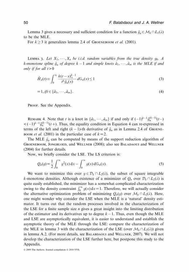
Lemma 3 gives a necessary and sufficient condition for a function gn ∈Mk ∩L1(�)to be the MLE.

For k ≥3 it generalizes lemma 2.4 of Groeneboom et al. (2001).

Lemma 3. Let X1, · · · , Xn be i.i.d. random variables from the true density g0. Ak-monotone spline gn of degree k −1 and simple knots a1, · · · , am is the MLE if andonly if for all t > 0

Hn(t)≡∫ ∞

0

k(t −x)k−1+

tk gn(x)dGn(x)≤1 (3)

=1, ift ∈{a1, · · · , am}. (4)

Proof. See the Appendix.

Remark 4. Note that t is a knot in {a1, · · · , am} if and only if (−1)k−1g(k−1)n (t−)

< (−1)k−1g(k−1)n (t +). Thus, the equality condition in Equation 4 can re-expressed in

terms of the left and right (k −1)-th derivative of gn as in Lemma 2.4 of Groene-boom et al. (2001) in the particular case of k =2.

The MLE gn can be computed by means of the support reduction algorithm ofGroeneboom, Jongbloed, and Wellner (2008); also see Baladaoui and Wellner(2004) for further details.

Now, we briefly consider the LSE. The LS criterion is:

Qn(g)= 12

∫ ∞

0g2(x) dx −

∫ ∞

0g(x) dGn(x). (5)

We want to minimize this over g ∈ Dk ∩ L2(�), the subset of square integrablek-monotone densities. Although existence of a minimizer of Qn over Dk ∩ L2(�) isquite easily established, the minimizer has a somewhat complicated characterizationowing to the density constraint

∫∞0 g(x) dx =1. Therefore, we will actually consider

the alternative optimization problem of minimizing Qn(g) over Mk ∩ L2(�). Here,one might wonder why consider the LSE when the MLE is a ‘natural’ density esti-mator. It turns out that the random processes involved in the characterization ofthe LSE for a finite sample size n gives a great insight into the limiting distributionof the estimator and its derivatives up to degree k −1. Thus, even though the MLEand LSE are asymptotically equivalent, it is easier to understand and establish theasymptotic theory of the MLE through the LSE: compare the characterization ofthe MLE in lemma 3 with the characterization of the LSE (over Mk ∩L2(�)) givenin lemma A.2. (For more details, see Balabdaoui and Wellner, 2007). We will notdevelop the characterization of the LSE further here, but postpone this study to theAppendix.© 2009 The Authors. Journal compilation © 2010 VVS.


3 Consistency

In this section, we will prove that both the MLE and LSE are strongly consistent.Furthermore, we will show that this consistency is uniform on intervals of the form[c, ∞), where c > 0.

Consistency of the MLEs for the classes Dk in the sense of Hellinger convergenceof the mixed density is a relatively simple straightforward consequence of the meth-ods of Pfanzagl (1988) and van de Geer (1993). As usual, the Hellinger distance His given by H2(p, q)= (1/2)

∫(√

p−√q)2d� for any common dominating measure �.

Proposition 1. Suppose that gn is the MLE of g0 in the class Dk. Then,

H(gn, g0)→a.s. 0 as n→∞.

Furthermore, F n →d F0 almost surely where F n is the MLE of the mixing distri-bution function F0

Proof. Note that math Dk ={gF : F is a d.f. on (0, ∞)} with

gF (x)=g(x)=∫ ∞

0kx(t) dF (t)

and kx is the the scaled beta(1, k) kernel; that is, kx(t)= t(1 − tx/k)k−1+ . For all x > 0,

the kernel kx is bounded, continuous, and it is easy to see that it satisfies limt↘0kx(t)=limt→∞kx(t)=0. Hence, the map F �→ gF is continuous with respect to the vaguetopology for all x > 0. This implies that the class

G ={

gF

gF +gF0

, F is a d.f. on (0, ∞)}

is continuous in F with respect to the vague topology for every x > 0. Now, as thefamily of sub-distributions F on (0, ∞) is compact for the vague topology (see, e.g.,Bauer, 1981), and the class G is uniformly bounded by 1, we conclude by lemma5.1 of van der Geer (1993) that g is P0-Glivenko–Cantelli. It follows by corollary 1of van der Vaart and Wellner (2000) that H(gn, g0)→a.s. 0. The second assertionof the proposition follows from lemma 5.2 of van de Geer (1993).

Lemma 4 establishes a useful bound for k-monotone densities.

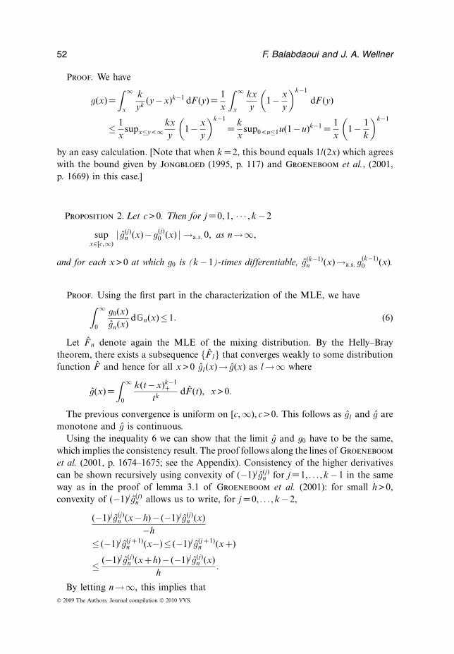
Lemma 4. If g is a k-monotone density function for k ≥2, then

g(x)≤ 1x

(1− 1

k

)k−1

for all x > 0.© 2009 The Authors. Journal compilation © 2010 VVS.


Proof. We have

g(x)=∫ ∞

x

kyk (y −x)k−1 dF (y)= 1

x

∫ ∞

x

kxy

(1− x

y

)k−1

dF (y)

≤ 1x

supx≤y <∞kxy

(1− x

y

)k−1

= kx

sup0 < u≤1u(1−u)k−1 = 1x

(1− 1

k

)k−1

by an easy calculation. [Note that when k =2, this bound equals 1/(2x) which agreeswith the bound given by Jongbloed (1995, p. 117) and Groeneboom et al., (2001,p. 1669) in this case.]

Proposition 2. Let c > 0. Then for j =0, 1, · · · , k −2

supx∈[c,∞)

| g(j)n (x)−g(j)

0 (x) | →a.s. 0, as n→∞,

and for each x > 0 at which g0 is (k −1)-times differentiable, g(k−1)n (x)→a.s. g

(k−1)0 (x).

Proof. Using the first part in the characterization of the MLE, we have∫ ∞

0

g0(x)gn(x)

dGn(x)≤1. (6)

Let F n denote again the MLE of the mixing distribution. By the Helly–Braytheorem, there exists a subsequence {F l} that converges weakly to some distributionfunction F and hence for all x > 0 gl(x)→ g(x) as l →∞ where

g(x)=∫ ∞

0

k(t −x)k−1+

tk dF (t), x > 0.

The previous convergence is uniform on [c, ∞), c > 0. This follows as gl and g aremonotone and g is continuous.

Using the inequality 6 we can show that the limit g and g0 have to be the same,which implies the consistency result. The proof follows along the lines of Groeneboomet al. (2001, p. 1674–1675; see the Appendix). Consistency of the higher derivativescan be shown recursively using convexity of (−1)j g(j)

n for j =1, . . ., k −1 in the sameway as in the proof of lemma 3.1 of Groeneboom et al. (2001): for small h > 0,convexity of (−1)j g(j)

n allows us to write, for j =0, . . ., k −2,

(−1)j g(j)n (x −h)− (−1)j g(j)

n (x)−h

≤ (−1)j g(j +1)n (x−)≤ (−1)j g(j +1)

n (x +)

≤ (−1)j g(j)n (x +h)− (−1)j g(j)

n (x)h

.

By letting n→∞, this implies that© 2009 The Authors. Journal compilation © 2010 VVS.


(−1)jg(j)0 (x −h)− (−1)jg(j)

0 (x)−h

≤ lim infn→∞ (−1)j g(j +1)

n (x−)≤ lim supn→∞

(−1)j g(j +1)n (x +)

≤ (−1)jg(j)0 (x +h)− (−1)jg(j)

0 (x)h

.

By letting h ↘ 0, we conclude consistency of g(j)n (x), j =0, . . ., k − 1 for x ∈ (0, ∞).

Note that consistency of (−1)j g(j)n , j =1, . . ., k −2 is uniform on intervals of the form

[c, ∞) because of continuity of those derivatives. For k − 1, only pointwise strongconsistency of (−1)k−1g(k−1)

n can be claimed.We also have strong and uniform consistency of the LSE gn on intervals of the

form [c, ∞), c > 0. The relevant result and proof are deferred to the Appendix.

4 Asymptotic minimax risk lower bounds for the rates of convergence

In this section, our goal is to derive minimax lower bounds for the behavior of anyestimator of a k-monotone density g and its first k −1 derivatives at a point x0 forwhich the k-th derivative exists and is non-zero. The proof will rely on the basiclemma 4.1 of Groeneboom (1996); see also Jongbloed (2000). This basic methodseems to go back to Donoho and Liu (1987, 1991).

As before, let Dk denote the class of k-monotone densities on [0, ∞). Here is thenotation we will need. Consider estimation of the j-th derivative of g ∈Dk at x0 forj ∈{0, 1, . . ., k −1}. If T n is an arbitrary estimator of the real-valued functional T ofg, then the (L1-minimax risk based on a sample X1, . . ., Xn of size n from g whichis known to be in a suitable subset Dk,n of Dk is defined by

MMR1(n, T , Dk,n)= inftn supg∈Dk,nEg | T n −Tg | .

Here the infimum ranges over all possible measurable functions tn : Rn → R, andT n = tn(X1, . . ., Xn). When the subclasses Dk,n are taken to be shrinking to one fixedg0 ∈Dk, the minimax risk is called local at g0. The shrinking classes (parameterizedby �> 0) used here are Hellinger balls centered at g0:

Dk,n ≡Dk,n,� ={

g ∈Dk : H2(g, g0)= 12

∫ ∞

0(√

g(x)−√

g0(x))2 dx ≤ �/n}.

The behavior, for n →∞ of such a local minimax risk MMR1 will depend on n(rate of convergence to zero) and the density g0 toward which the subclasses shrink.Lemma 5 is the basic tool for proving such a lower bound.

Lemma 5. Assume that there exists some subset {gε : ε> 0} of densities in Dk,n suchthat, as ε↓0,

H2(gε, g0)≤ ε(1+o(1)) and |Tgε −Tg0 | ≥ (cε)r(1+o(1))

for some c > 0 and r > 0. Then© 2009 The Authors. Journal compilation © 2010 VVS.


sup�> 0

lim infn→∞ nrMMR1(n, T , Dk,n,�)≥ 1

4

( cr2e

)r.

Proof. See Groeneboom (1996) and Jongbloed (2000).Here is the main result of this section.

Proposition 3. Let g0 ∈ Dk and x0 be a fixed point in (0, ∞) such that g0 isk-times continuously differentiable at x0 (k ≥ 2). An asymptotic lower bound for thelocal minimax risk of any estimator T n,j for estimating the functional Tjg0 =g(j)

0 (x0),is given by:

sup�> 0

lim infn→∞ n

k−j2k +1 MMR1(n, Tj , Dk,n,�)≥

{|g(k)

0 (x0) | 2j +1g0(x0)k−j}1/(2k +1)

dk,j ,

where dk,j > 0, j ∈{0, . . ., k −1}. Here

dk,j = 14

(4

k − j2k +1

e−1)(k−j)/(2k +1) �(j)

k,1

(�k,2)(k−j)/(2k +1) ,

where

�k,2 =

⎧⎪⎪⎪⎨⎪⎪⎪⎩

24(k +1) (2k +3)(k +2)(k +1)2

((2(k +1))!)2

(4k +7)!((k−1)!)2((

kk/2−1

))2 , k even

24(k +2)(2k +3)(k +2)(

(2(k +1))!/2

(4k +7)!(k!)2((

k +1(k−1)/2

))2 , k odd.

Proposition 3 also yields lower bounds for estimation of the corresponding mixingdistribution function F at a fixed point.

Corollary 1. Let g0 ∈ Dk and let x0 be a fixed point in (0, ∞) such that g0 isk-times continuously differentiable at x0, k ≥2. Then, for estimating Tg0 =F0(x0) whereF0 is given in terms of g0 by 2,

sup�> 0

lim infn→∞ n1/2k +1MMR1(n, T , Dk,n,�)

≥{

|g(k)0 (x0) | 2k−1g0(x0)

}1/(2k +1) xk0

k!dk,k−1.

Proof. See the Appendix.Both the rates of convergence n(k−j)/(2k +1) and the dependence of our lower bound

on the constants g0(x0) and g(k)0 (x0) match with the known results for k =1 and k =2

owing to Groeneboom (1985) and Groeneboom et al. (2001), and reappears in thelimit distribution theory for k ≥3 in Balabdaoui and Wellner (2007).© 2009 The Authors. Journal compilation © 2010 VVS.


Appendix

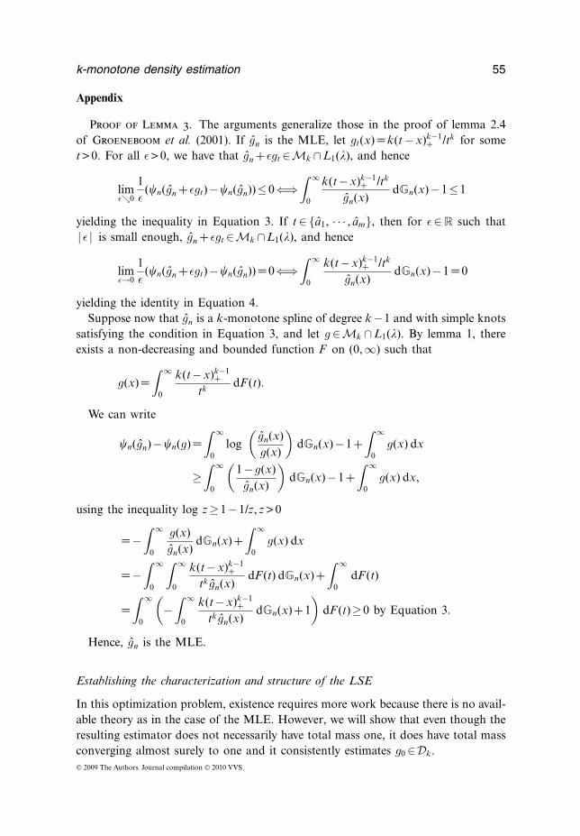
Proof of Lemma 3. The arguments generalize those in the proof of lemma 2.4of Groeneboom et al. (2001). If gn is the MLE, let gt(x)=k(t − x)k−1

+ /tk for somet > 0. For all ε> 0, we have that gn + εgt ∈Mk ∩L1(�), and hence

limε↘0

1ε

(�n(gn + εgt)−�n(gn))≤0⇐⇒∫ ∞

0

k(t −x)k−1+ /tk

gn(x)dGn(x)−1≤1

yielding the inequality in Equation 3. If t ∈ {a1, · · · , am}, then for ε ∈ R such that| ε | is small enough, gn + εgt ∈Mk ∩L1(�), and hence

limε→0

1ε

(�n(gn + εgt)−�n(gn))=0⇐⇒∫ ∞

0

k(t −x)k−1+ /tk

gn(x)dGn(x)−1=0

yielding the identity in Equation 4.Suppose now that gn is a k-monotone spline of degree k −1 and with simple knots

satisfying the condition in Equation 3, and let g ∈Mk ∩ L1(�). By lemma 1, thereexists a non-decreasing and bounded function F on (0, ∞) such that

g(x)=∫ ∞

0

k(t −x)k−1+

tk dF (t).

We can write

�n(gn)−�n(g)=∫ ∞

0log

(gn(x)g(x)

)dGn(x)−1+

∫ ∞

0g(x) dx

≥∫ ∞

0

(1−g(x)gn(x)

)dGn(x)−1+

∫ ∞

0g(x) dx,

using the inequality log z ≥1−1/z, z > 0

=−∫ ∞

0

g(x)gn(x)

dGn(x)+∫ ∞

0g(x) dx

=−∫ ∞

0

∫ ∞

0

k(t −x)k−1+

tk gn(x)dF (t) dGn(x)+

∫ ∞

0dF (t)

=∫ ∞

0

(−∫ ∞

0

k(t −x)k−1+

tk gn(x)dGn(x)+1

)dF (t)≥0 by Equation 3.

Hence, gn is the MLE.

Establishing the characterization and structure of the LSE

In this optimization problem, existence requires more work because there is no avail-able theory as in the case of the MLE. However, we will show that even though theresulting estimator does not necessarily have total mass one, it does have total massconverging almost surely to one and it consistently estimates g0 ∈Dk.© 2009 The Authors. Journal compilation © 2010 VVS.


Using arguments similar to those in the proof of theorem 1 in Williamson (1956),one can show that g ∈Mk if and only if

g(x)=∫ ∞

0(t −x)k−1

+ d�(t)

for a positive measure � on (0, ∞). Thus, we can rewrite the criterion Qn in termsof the corresponding measures �: by Fubini’s theorem∫ ∞

0g2(x) dx =

∫ ∞

0

∫ ∞

0rk(t, t′) d�(t) d�(t′)

where rk(t, t′)=∫ t∧t′

0 (t −x)k−1(t′ −x)k−1 dx, and∫ ∞

0g(x) dGn(x)=

∫ ∞

0

∫ ∞

0(t −x)k−1

+ d�(t) dGn(x)=∫ ∞

0sn,k(t) d�(t),

where sn,k(t)≡∫∞0 (t −x)k−1

+ dGn(x). Hence it follows that, with g =g�

Qn(g)= 12

∫ ∞

0

∫ ∞

0rk(t, t′) d�(t) d�(t′)−

∫ ∞

0sn,k(t) d�(t)≡�n(�).

Now, we want to minimize �n over the set X of all non-negative measures � on(0, ∞).

Proposition A.1. The functional �n admits a unique minimizer �, and hence theLSE gn exists and is unique.

Proof. Uniqueness follows from strict convexity of �n. To prove existence, it canbe shown that �n can be restricted to a subset C of X on which it is lower semicon-tinuous, and hence the minimization problem admits a solution by applying theorem38.B of Zeidler (1985, p. 152). In the following, we will exhibit the subset C, andshow that the conditions of Zeidler’s theorem are satisfied.

We begin by checking the hypotheses of Zeidler’s theorem 38.B (Zeidler, p. 1521985). We identity X of Zeidler’s theorem with the space X of non-negativemeasures on [0, ∞), and we show that we can take M of Zeidler’s theorem to be

C ≡{�∈X :�(t, ∞)≤Dt−(k−1/2)}for some constant D <∞.

First, we can, without loss, restrict the minimization to the space of non-negativemeasures on [X(1), ∞), where X(1) > 0 is the first-order statistic of the data. To seethis, note that we can decompose any measure � as �=�1 +�2, where �1 is concen-trated on [0, X(1)) and �2 is concentrated on [X(1), ∞). As the second term of Qn iszero for �1, the contribution of the �1 component to Qn(�) is always non-negative,so we make inf Qn(�) no larger by restricting to measures on [X(1), ∞).

We can restrict further to measures � with∫∞

0 tk−1 d�(t) ≤ D for some finiteD=D�. To show this, we first give a lower bound for rk(s, t). For s, t≥ t0 > 0 we have© 2009 The Authors. Journal compilation © 2010 VVS.


rk(s, t)≥ (1− e−v0 )t0

2ksk−1tk−1, (A.1)

where v0 ≈1.59. To prove Equation A.1, we will use the inequality

(1− v/k)k−1 ≥ e−v, 0≤ v≤ v0, k ≥2. (A.2)

[This inequality holds by straightforward computation; see Hall and Wellner (1979),especially their proposition 2.]

Thus, we compute

rk(s, t)=∫ ∞

0(s −x)k−1

+ (t −x)k−1+ dx

= 1k

sk−1tk−1∫ ∞

0

(1− y

sk

)k−1

+

(1− y

tk

)k−1

+dy

≥ 1k

sk−1tk−1∫ v0(t∧s)

0e−y/se−y/t dy

= 1k

sk−1tk−1 1c

∫ v0(t∧s)

0ce−cy dy, c ≡1/s +1/t

= 1k

sk−1tk−1 1c

(1− exp(−c(t ∧ s)v0)

)≥ 1

ksk−1tk−1 1

c

(1− exp(−v0)

)as

c(s ∧ t)= s + tst

(s ∧ t)={

(t + s)/t, s ≤ t(t + s)/s, s ≥ t

}≥1.

But, we also have

1c

= 1(1/s)+ (1/t)

= sts + t

≥ 12

s ∧ t ≥ 12

t0

for s, t ≥ t0, so we conclude that Equation A.1 holds.From the inequality A.1, we conclude that for measures � concentrated on [X(1), ∞)

we have

∫ ∫rk(s, t) d�(s) d�(t)≥ (1− e−v0 )X(1)

2k

(∫ ∞

0tk−1 d�(t)

)2

.

In contrast,

∫ ∞

0sn,k(t) d�(t)≤

∫ ∞

0tk−1 d�(t).



Combining these two inequalities it follows that for any measure � concentratedon [X(1), ∞) we have

�n(�)= 12

∫ ∫rk(t, s) d�(t) d�(s)−

∫ ∞

0sn,k(t) d�(t)

≥ (1− e−v0 )X(1)

4k

(∫ ∞

0tk−1 d�(t)

)2

−∫ ∞

0tk−1 d�(t)

≡Am2k−1 −mk−1.

This lower bound is strictly positive if

mk−1 > 1/A= 4k(1− e−v0 )X(1)

.

But for such measures � we can make � smaller by taking the zero measure. Thus,we may restrict the minimization problem to the collection of measures � satisfying

mk−1 ≤1/A. (A.3)

Now we decompose any measure � on [X(1), ∞) as �=�1 +�2 where �1 is concen-trated on [X(1), MX(n)] and �2 is concentrated on (MX(n), ∞) for some (large) M > 0.Then, it follows that

�n(�)≥ 12

∫ ∫rk(t, s) d�2(t) d�2(s)−

∫ ∞

0tk−1 d�(t)

≥ (1− ev0 )MX(n)

4k(MX(n))2k−2�(MX(n), ∞)2 −1/A

≡B�(MX(n), ∞)2 −1/A > 0

if

�(MX(n), ∞)2 >1

AB= 4k

(1− e−v0 )X(1)

4k(1− e−v0 )(MX(n))2k−1 ,

and hence we can restrict to measures � with

�(MX(n), ∞)≤ 4k

(1− e−v0 )X 1/2(1) X k−1/2

(n)

1Mk−1/2

for every M ≥1.But this implies that � satisfies∫ ∞

0tk−3/4 d�(t)≤D

for some 0 < D=D� <∞, and this implies that tk−1 is uniformly integrable over �∈C.Alternatively, for �≥1 we have



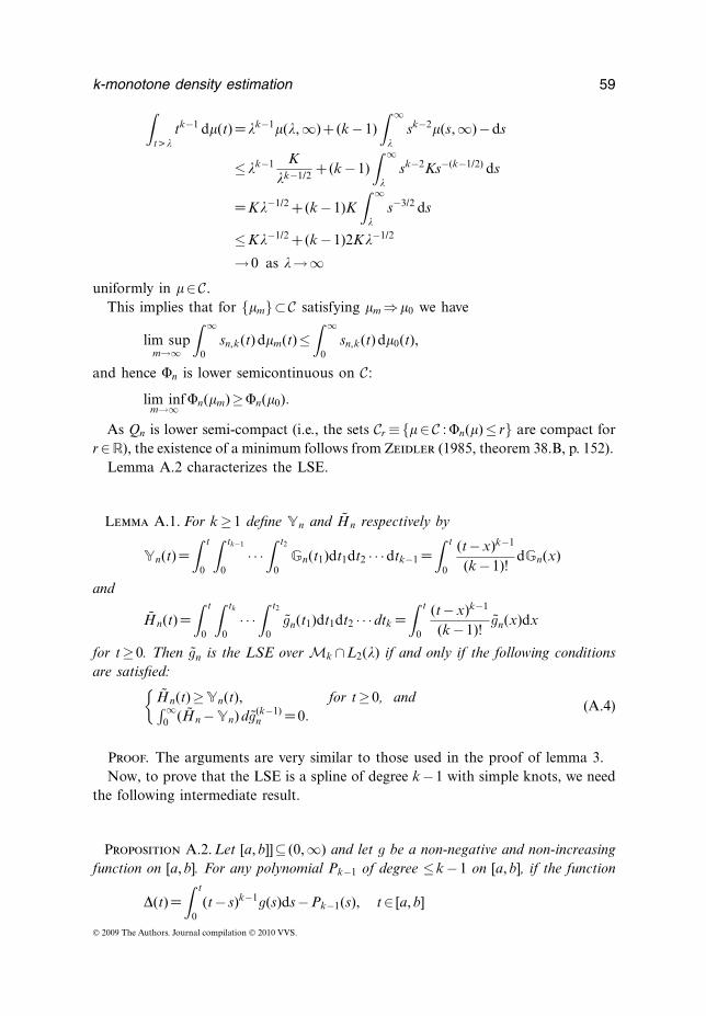
∫t >�

tk−1 d�(t)=�k−1�(�, ∞)+ (k −1)∫ ∞

�sk−2�(s, ∞)−ds

≤�k−1 K�k−1/2 + (k −1)

∫ ∞

�sk−2Ks−(k−1/2) ds

=K�−1/2 + (k −1)K∫ ∞

�s−3/2 ds

≤K�−1/2 + (k −1)2K�−1/2

→0 as �→∞uniformly in �∈C.

This implies that for {�m}⊂C satisfying �m ⇒�0 we have

lim supm→∞

∫ ∞

0sn,k(t) d�m(t)≤

∫ ∞

0sn,k(t) d�0(t),

and hence �n is lower semicontinuous on C:

lim infm→∞ �n(�m)≥�n(�0).

As Qn is lower semi-compact (i.e., the sets Cr ≡{� ∈C : �n(�) ≤ r} are compact forr ∈R), the existence of a minimum follows from Zeidler (1985, theorem 38.B, p. 152).

Lemma A.2 characterizes the LSE.

Lemma A.1. For k ≥1 define Yn and Hn respectively by

Yn(t)=∫ t

0

∫ tk−1

0· · ·∫ t2

0Gn(t1)dt1dt2 · · ·dtk−1 =

∫ t

0

(t −x)k−1

(k −1)!dGn(x)

and

Hn(t)=∫ t

0

∫ tk

0· · ·∫ t2

0gn(t1)dt1dt2 · · ·dtk =

∫ t

0

(t −x)k−1

(k −1)!gn(x)dx

for t ≥0. Then gn is the LSE over Mk ∩L2(�) if and only if the following conditionsare satisfied:{

Hn(t)≥Yn(t), for t ≥0, and∫∞0 (Hn −Yn) dg(k−1)

n =0.(A.4)

Proof. The arguments are very similar to those used in the proof of lemma 3.Now, to prove that the LSE is a spline of degree k −1 with simple knots, we need

the following intermediate result.

Proposition A.2. Let [a, b]]⊆ (0, ∞) and let g be a non-negative and non-increasingfunction on [a, b]. For any polynomial Pk−1 of degree ≤k −1 on [a, b], if the function

�(t)=∫ t

0(t − s)k−1g(s)ds −Pk−1(s), t ∈ [a, b]



admits infinitely many zeros in [a, b], then there exists t0 ∈ [a, b] such that g ≡ 0 on[t0, b] and g > 0 on [a, t0) if t0 > a.

Proof. By applying the mean value theorem k times, it follows that (k −1)!g =�(k)

admits infinitely many zeros in [a, b]. But as g is assumed to be non-negative andnon-increasing, this implies that if t0 is the smallest zero of g in [a, b], then g≡0 on[t0, b]. By definition of t0, g > 0 on [a, t0) if t0 > a.

Now we will use the characterization of the LSE gn together with the previousproposition to show that it is a finite mixture of beta(1, k)s. We know from lemmaA.1 that gn is the LSE if and only if Equation A.4 holds. The equality conditionin the second part of equation A.4 implies that Hn and Yn have to be equal atany point of increase of the monotone function (−1)k−1g(k−1)

n . Therefore, the set ofpoints of increase of (−1)k−1g(k−1)

n is included in the set of zeros of the function�n = Hn −Yn.

Now, note that Yn can be given by the explicit expression:

Yn(t)= 1(k −1)!

1n

n∑j =1

(t −X(j))k−1+ , for t > 0.

In other words, Yn is a spline of degree k −1 with simple knots at X(1), . . ., X(n),the order statistics of X1, . . ., Xn. Also note that the function (−1)k−1g(k−1)

n cannothave a positive density with respect to Lebesgue measure �. Indeed, if we assumeotherwise, then we can find 0 ≤ j ≤ n and an interval I ⊂ (X(j), X(j +1))(with X(0) =0and X(n+1) =∞) such that I has a non-empty interior, and Hn ≡ Yn on I. This

implies that H(k)n ≡Y(k)

n ≡0, as Yn is a polynomial of degree k −1 on I, and hencegn ≡ 0 on I. But the latter is impossible as it was assumed that (−1)k−1g(k−1)

n wasstrictly increasing on I. Thus, the monotone function (−1)k−1g(k−1)

n can have onlytwo components: discrete and singular. In the following, we will prove that it is actu-ally discrete with finitely many points of jump.

Proposition A.2. There exists m ∈ N \ {0}, a1, · · · , am and w1, · · · , wm such thatfor all x > 0, the LSE gn is given by

gn(x)= w1k(a1 −x)k−1

+ak

1

+ · · ·+ wmk(am −x)k−1

+ak

m

. (A.5)

Consequently, the equality part in Equation A.4 can be re-expressed as Hn(t)=Yn(t)if t is a point in the support of the minimizing (mixing) measure F n (or a knot of gn).

Proof. We need to consider two cases:(i) The number of zeros of �n = Hn − Yn is finite. This implies by the equality

condition in Equation A.4 that the number of points of increase of (−1)k−1g(k−1)n is



also finite. Therefore, (−1)k−1g(k−1)n is discrete with finitely many jumps and hence

gn is of the form given in Equation A.5.(ii) Now, suppose that �n has infinitely many zeros. Let j be the smallest inte-

ger in {0, · · · , n − 1} such that [X(j), X(j +1)] contains infinitely many zeros of �n,k

(with X(0) =0 and X(n+1) =∞). By proposition A.2, if tj is the smallest zero of gn in[X(j), X(j +1)], then gn ≡0 on [tj , X(j +1)] and gn > 0 on [X(j), tj) if tj > X(j). Note that fromthe proof of proposition A.1, we know that the minimizing measure �n does not putany mass on (0, X(1)], and hence the integer j has to be strictly greater than 0.

Now, by definition of j, �n has finitely many zeros to the left of X(j), which impliesthat (−1)k−1g(k−1)

n has finitely many points of increase in (0, X(j)). We also know thatgn ≡0 on [tj , ∞). Thus we only need to show that the number of points of increaseof (−1)k−1g(k−1)

n in [X(j), tj) is finite, when tj > X(j). This can be argued as follows.Consider zj to be the smallest zero of �n in [X(j), X(j +1)). If zj ≥ tj , then we can-not possibly have any point of increase of (−1)k−1g(k−1)

n in [X(j), tj) because it wouldimply that we have a zero of �n that is strictly smaller than zj . If zj < tj , then for thesame reason, (−1)k−1g(k−1)

n has no point of increase in [X(j), zj). Finally, (−1)k−1g(k−1)n

cannot have infinitely many points of increase in [zj , tj) because that would implythat �n has infinitely many zeros in (zj , tj), and hence by lemma A.1, we can findt′j ∈ (zj , tj) such that gn ≡0 on [t′

j , tj ]. But, this is impossible as gn > 0 on [X(j), tj).

Proof of the identity g =g0 (proof of Proposition 2). For 0 <� < 1 define ��

=G−10 (1−�). Let ε> 0 be small so that ε<�ε.

By Equation 6, there exists a number Dε > 0 such that gl(�ε)≥Dε for sufficientlylarge l. To see this, note that Equation 6, implies that

1≥∫ ∞

0

g0(x)gl(x)

dGl(x)≥∫ ∞

�ε

g0(x)gl(x) dGl(x)≥ 1gl(�ε)

∫ ∞

�ε

g0(x) dGl(x),

and hence

lim infl

gl(�ε)≥ lim infl

∫ ∞

�ε

g0(x) dGl(x)=∫ ∞

�ε

g0(x) dG0(x) > 0,

by the choice of �ε, and the claim follows by taking Dε =∫∞

�εg0(x) dG0(x)/2. Hence,

by the bound in lemma 4, we have

gl(z)≤ 1z

(1− 1

k

)k−1

≡ ek

z, g0(z)≤ 1

z

(1− 1

k

)k−1

≡ ek

z.

It follows that g0/gl is uniformly bounded on the interval [ε, �ε]; that is, there existtwo constants cε and cε such that for all x ∈ [ε, �ε]

cε ≤g0(x)gl(x)

≤ cε.

In fact,© 2009 The Authors. Journal compilation © 2010 VVS.


g0(x)gl(x)

≤ g0(ε)gl(�ε)

≤ ε−1ek

Dε,

while

g0(x)gl(x)

≥ g0(�ε)gl(ε)

≥ g0(�ε)ε−1ek

Therefore,

g0(x)gl(x)

→ g0(x)g(x)

uniformly on [ε, �ε]. Using Equation 6, we have for sufficiently large l and∫ �ε

ε

g0(x)g(x)

dGl(x)≤∫ �ε

ε

(g0(x)gl(x)

+ ε

)dGl(x)≤1+ ε.

But as Gl converges weakly to G0 the distribution function of g0 and g0/g is con-tinuous and bounded on [ε, �ε]; we conclude that∫ �ε

ε

g0(x)g(x)

dG0(x)≤1+ ε.

Now, by Lebesgue’s monotone convergence theorem, we conclude that∫ ∞

0

g0(x)g(x)

dG0(x)≤1,

which is equivalent to∫ ∞

0

g20(x)g(x)

dx ≤1. (A.6)

Define �=∫∞0 g(x) dx. Then, h= �−1g is a k-monotone density. By Equation A.6,

we have that∫ ∞

0

g20(x)

h(x)dx = �

∫ ∞

0

g20(x)g(x)

dx ≤ �.

Now, consider the function

K (g)=∫ ∞

0

g20(x)g(x)

dx

defined on the class Cd of all continuous densities g on [0, ∞). Minimizing K isequivalent to minimizing∫ ∞

0

(g2

0(x)g(x)

+g(x))

dx.

It is easy to see that the integrand is minimized pointwise by taking g(x)=g0(x).Hence, infCd K (g)≥1. In particular, K (h)≥1 which implies that �=1.

Now, if g �=g0 at a point x, it follows that g �=g0 on an interval of positive length.Hence, g0 �=g ⇒K (g) > 1. We conclude that we have necessarily h= g =g0.© 2009 The Authors. Journal compilation © 2010 VVS.


Proposition A.4. Fix c > 0 and suppose that the true k-monotone density g0 sat-isfies

∫∞0 x−1/2g0(x) dx <∞. Then, ‖ gn −g0 ‖ 2 →a.s. 0,

supx∈[c,∞)

| g(j)n (x)−g(j)

0 (x) | →a.s. 0, as n→∞,

for j =0, 1, · · · , k − 2, and, for each x > 0 at which g0 is (k − 1)-times differentiable,g(k−1)

n (x)→a.s. g(k−1)0 (x). Here, ‖ · ‖2 denotes the L2-norm.

Proof. The main difficulty here is that the LSE gn is not necessarily a density inthat it may integrate to more than one; indeed it can be shown that

∫∞0 g1(x) dx =

((2k − 2)/k)(1 − 1/(2k − 1))k−2 > 1 for k ≥ 3. However, once we show that gn staysbounded in L2 with high probability, the proof of consistency will be much like theone used for k =2; that is, consistency of the LSE of a convex and decreasing density(see Groeneboom et al., 2001). The proof for k =2 is based on the very importantfact that the LSE is a density, which helps in showing that gn at the last jump point�n ∈ [0, ] of g′

n for a fixed > 0 is uniformly bounded. The proof would have beensimilar if we only knew that

∫∞0 gn(x) dx =Op(1).

Here we will first show that∫∞

0 g2n d�=Op(1). Note that the equality part in Equa-

tion (A.4) can be re-written as∫∞

0 g2n(x)dx =∫∞

0 gn(x)dGn(x) and hence√∫ ∞

0g2

n(x)dx =∫ ∞

0un(x)dGn(x), (A.7)

where un ≡ gn/ ‖ gn ‖ 2 satisfies ‖ un ‖ 2 =1. Take Fk to be the class of functions

Fk ={

g ∈Mk,∫ ∞

0g2d�=1

}.

In the following, we show that Fk has an envelope G ∈L1(G0).Note that for g ∈Fk we have

1=∫ ∞

0g2d�≥

∫ x

0g2d�≥xg2(x),

as g is decreasing. Therefore, g(x)≤1/√

x ≡G(x) for all x > 0 and g ∈Fk; that is Gis an envelope for the class Fk. As G ∈ L1(G0) (by our hypothesis) it follows fromthe strong law that∫ ∞

0un(x) dGn(x)≤

∫ ∞

0G(x) dGn(x)→a.s.

∫ ∞

0G(x) dG0(x), as n→∞

and hence by Equation A.7 the integral∫∞

0 g2nd� is bounded (almost surely) by some

constant Mk.Now we are ready to complete the proof. Let > 0 and �n be the last jump point

of g(k−1)n if there are jump points in the interval (0, ]; otherwise, we take �n to be 0.

To show that the sequence(gn(�n)

)n stays bounded, we consider two cases:



1. �n ≥/2. Let n be large enough so that∫∞

0 g2nd�≤Mk. We have

gn(�n)≤ gn(/2)= (2/)(/2)gn(/2)≤ (2/)∫ /2

0gn(x)dx

≤ (2/)√

/2

√∫ /2

0g2

n(x)dx ≤√

2/

√∫ ∞

0g2

n(x)dx

=√2Mk/. (A.8)

2. �n </2. We have∫

�n

gn(x)dx ≤√

− �n

√∫

�n

g2n(x)dx ≤

√

√∫ ∞

0g2

n(x)dx =√Mk.

Using that gn is a polynomial of degree k −1 on the interval [�n, ], we have

√Mk ≥

∫

�n

gn(x)dx = gn()(− �n)− g′n()2

(− �n)2 + · · ·+ (−1)k−1 g(k−1)n ()

k!(− �n)k

≥ (− �n)

(gn()+ 1

k(−1)g′

n()(− �n)+ · · ·+ (−1)k−1 g(k−1)n ()

(k −1)!(− �n)k−1

)

= (− �n)(

gn()(

1− 1k

)+ 1

kgn(�n)

)≥

2kgn(�n)

and hence gn(�n)≤2k√

Mk/. By combining the bounds, we have for large n, gn(�n)≤2k

√Mk/=Ck. Now, as gn() ≤ gn(�n), the sequence gn(x) is uniformly bounded

almost surely for all x ≥. Using a Cantor diagonalization argument, we can find asubsequence {nl} so that, for each x ≥, gnl (x)→ g(x), as l →∞. By Fatou’s lemma,we have∫ ∞

(g(x)−g0(x))2dx ≤ lim inf

l→∞

∫ ∞

(gnl

(x)−g0(x))2dx. (A.9)

However, the characterization of gn implies that Qn(gn)≤Qn(g0), and this yields∫ ∞

0(gn(x)−g0(x))2dx ≤2

∫ ∞

0(gn(x)−g0(x))d(Gn(x)−G0(x)).

Thus, we can write∫ ∞

(gnl

(x)−g0(x))2dx ≤∫ ∞

0(gnl

(x)−g0(x))2dx

≤2∫ ∞

0(gnl

(x)−g0(x))d(Gnl (x)−G0(x))→a.s. 0,(A.10)

as l →∞. The last convergence is justified as follows: as∫∞

0 g2nl

d� is bounded almostsurely, we can find a constant C > 0 such that gnl

−g0 admits G(x)=C/√

x, x > 0, asan envelope. Since G ∈ L1(G0) by hypothesis and as the class of functions{(g − g0)1[G≤M ] : g ∈Mk ∩ L2(�)} is a Glivenko-Cantelli class for every M > 0 (each© 2009 The Authors. Journal compilation © 2010 VVS.


element is a difference of two bounded monotone functions) Equation A.10 holds.From Equation A.9, we conclude that

∫∞ (g(x)−g0(x))2dx≤0, and therefore, g≡g0

on (0, ∞) as > 0 can be chosen arbitrarily small. We have proved that there exists�0 with P(�0)=1 and such that for each �∈�0 and any given subsequence gnk

(·, �),we can extract a further subsequence gnl

(·, �) that converges to g0 on (0, ∞). Itfollows that gn converges to g0 on (0, ∞), and this convergence is uniform onintervals of the form [c, ∞), c > 0 by the monotonicity and continuity of g0. As forthe MLE, consistency of the higher derivatives can be shown recursively using theconvexity of (−1)j g(j)

n for j =1, . . ., k −2.

Proof of Proposition 3. Let � be a positive number and consider the functiong� defined by

g�(x)= (x0 +�−x)k +1(x −x0 +�)k +21[x0−�,x0 +�](x).

Now, consider the perturbation

g�(x)=g0(x)+ s(�)g�(x), x ∈ (0, ∞),

where s(�) is a scale to be determined later. If � is chosen small enough so thatthe true density g0 is k-times continuously differentiable on [x0 −�, x0 +�], the per-turbed function g� is also k-times differentiable on [x0 −�, x0 +�] with a continuousk-th derivative. Now, let r be the function defined on (0, ∞) by

r(x)= (1−x)k +1(1+x)k +21[−1,1](x)= (1−x2)k +1(1+x)1[−1,1](x).

Then, we can write g� as g�(x)=�2k +3r((x −x0)/�). Then, for 0≤ j ≤k

g(j)� (x0)−g(j)

0 (x0)= s(�)�2k +3−j r(j)(0).

The scale s(�) should be chosen so that (−1)jg(j)� (x) > 0 for all 0 ≤ j ≤ k, for x ∈

[x0 −�, x0 +�]. But for � small enough, the sign of (−1)jg(j)� will be that of (−1)jg(j)

0 (x0),and hence g� is k-monotone. For j =k, g(k)

� (x0)=g(k)0 (x0)+ s(�)�k +3r(k)(0). Assume

that r(k)(0) �=0. Set s(�)=g(k)0 (x0)/(�k +3r(k)(0)). Then, for 0≤ j ≤k −1

g(j)� (x0)=g(j)

0 (x0)+�k−j g(k)0 (x0)r(j)(0)

r(k)(0)=g(j)

0 (x0)+o(�),

as �→0, and

(−1)kg(k)� (x0)=2(−1)kg(k)

0 (x0) > 0.

To compute r(j)(0), note that for m≥2 and 2n≥m we have((1−x2)n)(m) = (((1−x2)n)′

)(m−1)

= (−2nx(1−x2)n−1)(m−1)

=−2n(x((1−x2)n−1)(m−1) + (m−1)((1−x2)n−1)m−2) ,



where in the last equality we used Leibniz’s formula for the derivatives of a prod-uct; see, for example, Apostol (1957, p. 99). Evaluating the last expression at x =0yields

xn,m ≡ ((1−x2)n)(m)∣∣∣∣x =0

=−2n(m−1)xn−1,m−2.

If m is even, we find that

xn,m = (−2)m/2m/2−1∏

i =0

(n− i)×m/2−1∏

i =0

(m−2i −1)×xn−m/2,0

= (−2)m/2m/2−1∏

i =0

(n− i)×m/2−1∏

i =0

(m−2i −1)

as xn−m/2,0 =1. Similarly, when m is odd,

xn,m = (−2)(m−1)/2(m−1)/2−1∏

i =0

(n− i)×(m−1)/2−1∏

i =0

(m−2i −1)×xn−(m−1)/2,1

=0

as xn−(m−1)/2,1 =0. Now we have, for 1≤ j ≤k,

r(j)(x)= ((1−x2)k +1(1+x))(j)

= (x +1)((1−x2)k +1)(j) + j

((1−x2)k +1)(j−1)

and hence

r(j)(0)= ((1−x2)k +1)(j)∣∣∣∣x =0

+ j((1−x2)k +1)(j−1)

∣∣∣∣x =0

.

Therefore, when j is even the second term vanishes and

r(j)(0)= (−2)j/2j/2−1∏i =0

(k +1− i)×j/2−1∏j =0

(j −2i −1) �=0.

When j is odd, the first term vanishes and

r(j)(0)= (−2)(j−1)/2(j−1)/2−1∏

i =0

(k +1− i)×(j−1)/2∏

i =0

(j −2i) �=0.

Summarizing, we have shown that

r(j)(0)={

(−2)j/2∏j/2−1i =0 (k +1− i)×∏j/2−1

i =0 (j −2i −1) �=0 j even(−2)(j−1)/2∏(j−1)/2−1

i =0 (k +1− i)×∏(j−1)/2i =0 (j −2i) �=0 j odd.

We set Ck,j = r(j)(0) for 1≤ j ≤k. Then, Ck,k becomes

Ck,k ={

(−2)k/2∏k/2−1i =0 (k +1− i)×∏k/2−1

i =0 (k −2i −1) if k is even(−2)(k−1)/2∏(k−1)/2−1

i =0 (k +1− i)×∏(k−1)/2i =0 (k −2i) if k is odd.



The previous expressions can be given in a more compact form. After some alge-bra, we find that

Ck,k ={

2× (−1)k/2(k +1)(k −1)!( k

k/2−1

)if k is even

(−1)(k−1)/2k!( k +1

(k−1)/2

)if k is odd.

(A.11)

We have for 0≤ j ≤k −1,

|Tj(g�)−Tj(g0)|=∣∣∣∣Ck, j

Ck, kg(k)

0 (x0)

∣∣∣∣�k−j ≡�(j)k,1

∣∣g(k)0 (x0)

∣∣�k−j ,

where we defined �(j)k,1 = |Ck,j /Ck,k| for j ∈{0, . . ., k − 1}. Furthermore, by computa-

tion and change of variables,

∫ ∞

0

(g�(x)−g0(x))2

g0(x)dx =

⎛⎜⎝(g(k)

0 (x0))2

g0(x0)

∫ 1−1(1− z2)2(k +1)(z +1)2dz

(Ck,k)2

⎞⎟⎠�2k +1 +o(�2k +2)

as �↘0. This gives control of the Hellinger distance as well in view of Jongbloed(2000, lemma 2, p. 282), or Jongbloed (1995, corollary 3.2, pp. 30–31). We set

�k, 2 =∫ 1

−1(1− z2)2(k +1)(z +1)2dz

(Ck, k)2

=

⎧⎪⎪⎨⎪⎪⎩

24(k +1) (2k +3)(k +2)(k +1)2

((2(k +1)))2

(4k +7)((k−1))2(( k

k/2−1/)2 k even

24(k +2)(2k +3)(k +2) ((2(k +1)))2

(4k +7)(k)2(( k +1

(k−1)/2/)2 k odd.

Now, by using the change of variable ε=�2k +1(bk +o(1)), where

bk =�k,2(g(k)0 (x0))2/g0(x0))

so that �= (ε/bk)1/(2k +1)(1+o(1)), then for 0≤ j ≤k −1, the modulus of continuity,mj , of the functional Tj satisfies

mj(ε)≥�(j)k,1g

(k)0 (x0)

(ε

bk

)(k−j)/(2k +1)

(1+o(1)).

The result is that mj(ε)≥ (rk,jε)(k−j)/2k+1/(1+o(1)), where rk,j =(�(j)k,1g

(k)0 (x0))(2k+1)/(k−j)/bk

and hence

sup�> 0

limn→∞ inf n(k−j)/(2k +1)MMR1(n, Tj , Dk,n,�)

≥ 14

(4

k − j2k +1

e−1)(k−j)/(2k +1)

(rk,j)(k−j)/(2k +1),(A.12)

which can be rewritten as

sup�> 0

limn→∞ inf n(k−j)/(2k +1)MMR1(n, Tj , Dk,n,�)

≥ 14

(4

k − j2k +1

e−1)(k−j)/(2k +1) �(j)

k,1

(�k,2)(k−j)/(2k +1)

{∣∣g(k)0 (x0)

∣∣(2j +1)/(2k +1)g0(x0)(k−j)/(2k +1)

}© 2009 The Authors. Journal compilation © 2010 VVS.


for j =0, · · · , k − 1. Finally, note that the fact that the function g� is not exactly adensity will not affect the obtained constants its integral converges to 1 as �→0.

Proof of Corollary 1. Let G�(x)=∫ x0 g�(t)dt. Using the inversion formula in

Equation 2, we have

T (g�)−T (g0)=G�(x0)−G0(x0)+k∑

j =1

(−1)j xj0

j!(Tj−1(g�)−Tj−1(g0)).

For j =1, . . ., k, we have already established before that |Tj−1(g�) − Tj−1(g0) | =�(j)

k,1 |g(k)0 (x0) |�k−j . In constrast, we have for � > 0 small enough

G�(x0)=G0(x0)+ s(�)∫ x0 +�

x0−�(x0 +�−x)k +1(x −x0 +�)k +2dx

=G0(x0)+ s(�)∫ x0 +�

x0−�(x −x0 +�)k +1(x −x0 −�)k +1dx

=G0(x0)+ s(�)∫ 1

−1r(x)dx�2k +4

=G0(x0)+ g(k)0 (x0)

�k +3r(k)(0)

(∫ 1

−1r(x)dx

)�2k +4

=G0(x0)+O(�k +1)).

Hence,

|T (g�)−T (g0) | = xk0

k!�(k−1)

k,1 |g(k)0 (x0) |�+o(�).

Using again the change of variable ε=�2k +1(bk +o(1)), we obtain the claimedlower bound in the same way as in proprosition 3.

Acknowledgements

The research of the second author was supported in part by NSF grants DMS-0203320 and DMS-0503822, and by NI-AID grant 2R01 AI291968-04. The authorsgratefully acknowledge helpful conversations with Carl de Boor, Nira Dyn, TilmannGneiting and Piet Groeneboom.

References

Anevski, D. (1994), Estimating the derivative of a convex density, Technical Report 1994:8,Department of Mathematical Statistics, University of Lund.

Anevski, D. (2003), Estimating the derivative of a convex density, Statistica Neerlandica 57,245–257.



Apostol, T. M. (1957), Mathematical analysis: a modern approach to advanced calculus, Addi-sion-Wesley Publishing Company, Inc., Reading, MA.

Ayer M., H. D. Brunk, G. M. Ewing, W. T. Reid and E. Silverman (1955), An empirical dis-tribution function for sampling with incomplete information, The Annals of MathematcialStatistics 26, 641–647.

Balabdaoui, F. (2007), Consistent estimation of a convex density at the origin, MathematicalMethods of Statistics 16, 77–95.

Balabdaoui, F. and J. A. Wellner (2004), Estimation of a K-monotone density, part 2: algo-rithm for computation and numerical results, Technical Report 460, Department of Statistics,University of Washington.

Balabdaoui, F. and J. A. Wellner (2007), Estimation of a K-monotone density: Limit dis-tribution theory and the spline connection, The Annals of Statistics 35, 2536–2564.

Brunk H. D. (1981), Probability theory and elements of measure theory, Academic Press Inc.[Harcourt Brace Jovanovich Publisher], London. Second edition of the translation by R. B.Burckel from the third German edition, Probability and Mathematical Statistics.

Brunk H. D. (1958), On the estimation of parameters restricted by inequalities. Annals ofMathematical Statistics 29, 437–454.

De Boor, C. (1978), A practical guide to splines, vol. 27 of Applied Mathematical Science,Springer-Verlag, New York.

DeVore, R. A. and G. G. Lorentz (1993), Constructive approximation, vol. 303 of Grundleh-ren der Mathematischen Wissenschaften [Fundamental Principles of Mathematical Sciences],Springer-Verlag Berlin.

Donoho, D. L. and R. C. Liu (1987), Geometrizing rates of convergence. i, Technical Report.137, Department of Statistics, University of Califonia, Berkeley.

Donoho, D. L. and R. C. Liu (1991), Geometrizing rates of convergence. II III, The Annalsof Statistics 19, 633–667, 668–701.

van Eeden, C. (1957a), Maximum likelihood estimation of partially or completely orderedparameters. I, Koninklijke Nederlandse Akademie van Wetenschappen Proceedings. Series AMathematical Sciences 19, 128–136.

van Eeden, C. (1957b), Maximum likelihood estimation of partially or completely orderedparameters. II, Koninklijke Nederlandse Akademie van Wetenschappen Proceedings. Series AMathematical Sciences 19, 201–211.

Feller, W. (1971), An introduction to probability theory and its applications, vol. II, 2nd edi-tion, John Wiley & Sons Inc., New york.

van de Geer, S. (1993), Hellinger-consistency of certain nonparametric maximum likelihoodestimators, The Annals of Statistics 21, 14–44.

Gneiting, T. (1998), On the Bernstein–Hausdorff–Widder conditions for completely mono-tone function. Expositionces Mathaticae 16, 88–119.

Gneiting, T. (1999), Radial positive definite functions generated by Euclid’s hat, Journal ofMultivariate Analysis 69, 88–119.

Grenander, U. (1956a), On the theory of mortality measurement. I Skandinavisk Aktuarietid-skrift 39, 70–96.

Grenander, U. (1956b), On the theory of mortality measurement. II, Skandinavisk Aktuari-etidskrift 39, 125–153.

Groeneboom, P. (1985), Estimating a monotone density, in: Proceedings of the Berkeley con-ference in honor of Jerzy Neyman and Jack Kiefer Vol. II (Berkeley, CA. 1983), WadsworthStatist./Probab. Ser., Wadsworth, Belmont, CA.

Groeneboom, P. (1989), Brownian motion with a parabolic drift and Airy functions, Proba-bility Theory and Related Fields 81, 79–109.

Groeneboom, P. (1996), Lectures on inverse problems, in: Lectures on probability theory andstatistics (Saint-Flour 1994), vol. 1648 of Lecture Notes in Mathematics, Springer, Berlin,pp. 67–164.

Groeneboom, P., G. Jongbloed and J. A. Wellner (2001), Estimation of a convex function:characterizations and asymptotic theory, The Annals of Statistics 29, 1653–1698.



Groeneboom, P., G. Jongbloed and J. A. Wellner (2008), The support reduction algorithmfor computing non-parametric function estimates in mixture models, Scandinavian Journalof Statistics 35, 385–399.

Hall, W. J. and J. A. Wellner (1979), The rate of convergence in law of the maximum of anexponential sample, Statistica Neerlandica 33, 151–154.

Hampel, F. R. (1987). Design modelling and anlysis of some biological datasets, in: design,data and analysis, by some friends of Cuthbert Daniel C. Mallows (ed.), Wiley, New york,pp. 111–115.

Jewell, N. P. (1982), Mixtures of exponential distributions, The Annals of Statistics 10, 479–484.

Jongbloed, G. (1995), Three statistical inverse problems, Ph.D. Thesis, Delft University ofTechnology.

Jongbloed, G. (2000), Minimax lower bounds and moduli of continuity, Statistics & Proba-bility Letters 50, 279–284.

Kim, J. and D. Pollard (1990), Cube root asymptotics, The Annals of Statistics 18, 191–219.Lévy, P. (1962) Extensions d’un théorème de D. Dugué et M, Girault. Probability Theory and

Related Fields 1, 159–173.Lindsay, B. G. (1983), The geometry of mixture likelihoods: a general theory, The Annals of

Statistics 11, 86–94.Pfanzagl, J. (1988), Consistency of maximum likelihood estimators for certain nonparametric

families in particular: mixtures, Journal of Statistical Planning and Inference 19, 137–158.Prakasa Rao, B. L. S. (1969), Estimation of a unimodal density, Sankhya Series A 31, 23–36.Silverman, B. W. (1982), On the estimation of a probability density function by the maximum

penalized likelihood method, The Annals of Statistics 10, 795–810.van der vaart, A. and J. A. Wellner (2000), Preservation theorems for Glivenko-Cantelli and

unifrom Gilvenko-Cantelli classes, in: Hign dimensional probability, II (Seattle, WA, 1999),vol. 47 of Progr. Probab., BirKhäuser Boston, Boston, MA, pp. 115–133.

Vardi, Y. (1989), Multiplicative censoring, renewal process, deconvolution and decreasing den-sity: nonparametric estimation, Biometrika 76, 751–761.

Williamson R. E. (1956), Multiply monotone functions and their Laplace transforms, DukeMathematical Journal 23, 189–207.

Woodroofe, M. and J. Sun (1993), A penalized maximum likelihood estimate of f(0+) whenf is nonincreasing, Statistics Sinica 3, 501–515.

Zeidler, E. (1985), Nonlinear functional analysis and its applications. III, Springer-Verlag, Newyork: Variational methods and optimization Translated from German by Leo F. Boron.

Received: September 2008. Revised: September 2009.


Estimation of a k -monotone density: characterizations, consistency and minimax lower bounds

Documents

Transcript of Estimation of a k -monotone density: characterizations, consistency and minimax lower bounds