No. 025/2020/POM/DEC A Minimax Regret Model for Leader ...

No. 025/2020/POM/DEC

A Minimax Regret Model for Leader-Follower Facility Location Problem

Xiang Li

School of Economics and Management

Beijing University of Chemical Technology

Tianyu Zhang



Liang Wang

Department of Economics and Decision Sciences

China Europe International Business School (CEIBS)

Hongguang Ma*



Xiande Zhao

Department of Economics and Decision Sciences

China Europe International Business School (CEIBS)

July 2020

––––––––––––––––––––––––––––––––––––––––

* Corresponding author: Hongguang Ma ([email protected]). Address: School of Economics and Management,

Beijing University of Chemical Technology, 15 Beisanhuan East Road, Chaoyang, Beijing 100029, China. The

authors would like to thank financial support from National Natural Science Foundation of China (Grant No.

71722007) and “the Fundamental Research Funds for the Central Universities (XK1802-5)”.

mailto:[email protected]

Noname manuscript No.(will be inserted by the editor)

A minimax regret model for leader-follower facilitylocation problem

Xiang Li · Tianyu Zhang · Liang Wang ·Hongguang Ma∗ · Xiande Zhao

Received: date / Accepted: date

Abstract Leader-follower facility location problem is usually consisting of aleader and a follower, in which the two competitors are going to locate newfacilities sequentially. The traditional studies generally assume that the lead-er knows in advance the partial or full information about the follower’s re-sponse when he makes decision. This assumption, however, may be invalid orimpracticable in practice. In this paper, we consider that the leader needs tolocate a predetermined number of new facilities without knowing any informa-tion about the follower’s response. By separating scenarios on the follower’sresponse with different number of new facilities, a minimax regret model isproposed for the leader so that his maximum possible loss can be minimized.Based on the structural characteristics of the proposed model, a set of solvingprocedures is provided with transforming the follower’s nonlinear (fraction)programming model into a linear one. In the numerical experiments, the pro-posed model is compared to two other location model, deterministic model andrisk model, and the efficiency of linearization in decreasing the computation

Xiang LiSchool of Economics and Management, Beijing University of Chemical Technology, Beijing100029, China

Tianyu ZhangSchool of Economics and Management, Beijing University of Chemical Technology, Beijing100029, China

Liang WangChina Europe International Business School, 699 Hongfeng Road, Pudong, Shanghai 201206,China

Hongguang Ma(Corresponding author)School of Economics and Management, Beijing University of Chemical Technology, Beijing100029, China E-mail: [email protected]

Xiande ZhaoChina Europe International Business School, 699 Hongfeng Road, Pudong, Shanghai 201206,China

2 Xiang Li et al.

time is verified. The results reveal that the proposed model is more applicablefor the leader when there is no information about the number or probabilitydistribution of the follower’s new facilities.

Keywords Leader-follower facility location · Competition · Minimax regretmodel · Linearization

1 Introduction

The research on facility location problem begins with Weber’s (1909) famouspaper. After that, operations researchers, traffic engineers, economists, andothers have discussed the location of diverse facilities, such as service facility(Farahani et al., 2019; Xia et al., 2015), medical facility (Zhang and Atkins,2019), emergency facility (Sestayo and Castro, 2019), utility facility (Ahma-di et al., 2016) and so on. Hotelling (1929) analyzed the location choice andpricing decision of two competitors on a finite line with uniformly spread con-sumers, which differs from the classic facility location problem and is generallyagreed as the first paper on competitive facility location problem. In the fieldof competitive facility location studies, the authors incorporate the fact thatother facilities are already (or will be) in the market and that any new facili-ty(ies) will have to compete with them for its (their) market share (Plastria,2001).

For competitive facility location problem, the customer choice rule for pa-tronizing facilities is of great concern. The two mainly used rules are deter-ministic utility rule and random utility rule. Deterministic utility rule meansthat customers only visit the facility which gives them the highest utility, forexample they only visit the closest facility or the facility offering the cheap-est product. For random utility rule, customers are assumed to distributetheir demand with certain probability. Gravity-based rule proposed by Reilly(1931) and later used by Huff (1964) and Huff (1966) is the most widely usedrandom utility rule, in which customer’s probability to patronize a facility isproportional to the facility’s attractiveness and inversely proportional to thedistance between the customer and the facility. Some new customer choicerules are proposed in recent years. For example, Fernandez et al. (2017) pro-posed multi-deterministic utility rule (also named partially binary rules) intheir work, which assumes that customers neither visit only one facility nordistribute their demand to all facilities. They only visit the most attractivefacility in each company, and distribute their demand among all these mostattractive facilities according to the gravity-based rule. Kung and Liao (2018)explained that consumer’s demand are affected by the number of facilities,with the increasing number of new facilities, the total demand will grow. InFernandez et al. (2019), a probabilistic customer’s choice rule is proposed, inwhich customers only patronize those facilities for which they feel an attrac-tion greater than or equal to a threshold value. In this paper, we take theclassical gravity-based rule to deal with competitive facility location problem,which is the most widely used rule and the base of aforementioned new rules.

A minimax regret model for leader-follower facility location problem 3

According to competition pattern, the competitive facility location can beclassified into four categories (Kress and Pesch, 2012): (1) static competition,in which the competitors are fixed and the players know all information; (2)dynamic competition, in which players repeatedly reoptimize their locations;(3) simultaneous competition, in which two rational competitors make theirdecisions at the same time to reach Nash equilibrium; and (4) sequential com-petition, which includes two types of players, leaders who choose locations atgiven instants and followers who make their location decisions based on thepast decisions of the leaders. The solution concept generally employed in se-quential location problems is the Stackelberg equilibrium: assuming rationalplayers, and the location of each player is determined by backward induction.In this paper, we focus on the sequential competition and call it as leader-follower facility location problem in the rest of this paper.

Hakimi (1983) first introduced the leader-follower issue in the competi-tive facility location problem. He formally introduced the terms (r|p)-centroidproblem and (r|Xp)-medianoid problem with one leader and one follower lo-cating p and r facilities, respectively. In a (r|p)-centroid problem, the leaderwill locate p new facilities with the belief that the follower will invest r newfacilities later. The (r|Xp)-medianoid problem is to locate r new facilities forthe follower in order to maximize her market share, knowing that the leaderhas located p new facilities. Furthermore, Hakimi has proven that the leader-follower problems in (r|p)-centroid and (r|Xp)-medianoid cases are N-P hard.Moore and Bard (1990) pointed out that the leader and the follower alwaysconflict with each other when both of them aim to optimize their objectivefunctions, which means if one competitor’s market share grows, the other willdecrease.

Most researchers assumed that the leader knows exactly how many newfacilities will be opened by follower, such that the leader-follower problem canbe formulated as deterministic models. Hakimi (1986) solved the deterministicleader-follower model by relaxing the condition of fixed demand in a networkspace. Serra and ReVelle (1994) proposed two heuristic algorithms for leader-follower model, in which the leader and the follower locate the same numberof facilities and customers only choose to patronize the closest facility. Fis-cher (2002) formulated the model in discrete space with the assumption thataccurate number of new facilities will be built. The leader and the followerwant to decide the locations and also the price of product, and a heuristicalgorithm is developed to solve the problem. Perez and Pelegrın (2003) for-mulated a leader-follower model in a tree and assumed that only one facilityis to be located by both of them, two algorithms are proposed to generate alloptimal locations for the leader, then the entire set of Stackelberg solutionsare formed. Saiz et al. (2009) also assumed that the leader and the followeronly locate one facility, but they formulated the model in a continuous spaceand proposed a branch-and-bound method to solve their problem. Drezner andDrezner (1998) developed three heuristic methods to deal with a similar modelto Saiz et al. (2009). Qi et al. (2017) introduced service distance limitationsin the leader-follower issue with the assumption that both the leader and the

4 Xiang Li et al.

follower plan to open certain number of facilities. Gentile et al. (2018) con-sidered three pairs of objective functions for the leader and the follower withpredetermined number of facilities for them and branch-and-cut algorithmsare used to solve the proposed models. Some recent studies also consideredhow to decide service quality, radius of influence, product variety, routing andso on, but the number of follower’s new facilities is still deterministic in thesestudies (Aboolian et al., 2007; Saidani et al., 2012; Wang and Ouyang, 2013;Drezner et al., 2015; Redondo et al., 2015; Lopes et al., 2016; Sedghi et al.,2017; Dilek et al., 2018).

As the leader acts ahead of the follower and they are in competition, itis reasonable to assume that the leader has no information on the follower’snumber of new facilities in advance. Ashtiani et al. (2013) built a robust mod-el for the leader-follower problem with inaccurate number of follower’s newfacilities in a discrete space. They defined their model as risk model withknown probability distribution, which made a trade-off between expect valueand deviation of leader’s market share. After reviewing the literature on thistopic, this conclusion can be drawn that previous studies have modeled theleader’s problem with respect to the assumption that the number of follower’snew facilities are known or with known probability distribution. However, ina competitive market, the information of the number or the probability distri-bution of follower’s new facilities can not be captured easily by leader. Mostworsely, a wrong estimation on the probability distribution may lead to moreloss for the leader. A realistic example of leader-follower problem is about re-tail store location. Jingdong (JD), as one of the leading companies in China,has invested a considerable amount of capital to retail industry. According tothe CEO’s interview of JD, more than 1000 convenience stores were openedper week in 2018, and they aim to open 1000 stores in China each day in2019. At the same time, competitions are everywhere in the market. Thereare some local convenience store brands, who are the main competitors for JDin each province. For example, Everyday is a convenience store company inShanxi province, which opens some new stores each day since 2018, and theinformation of Everyday’s decision is unknown for JD.

The contributions of this paper include: (i) We propose a minimax regretmodel for the competitive facility location problem consisting of a leader anda follower, in which the leader has no idea in advance on the number or prob-ability distribution of the follower’s new facilities when he makes decision; (ii)Based on the structural characteristics of the proposed model, a set of solvingprocedures is provided with transforming the follower’s nonlinear (fraction)programming model into a linear one; (iii) The numerical experiments showthat the minimax regret model is brilliant when the number of follower’s re-sponse is unknown, by which we can better control the maximum possible losscompared to deterministic model and risk model.

The rest of this paper is organized as follows: In Section 2, a minimax re-gret model for leader-follower problem is formulated. In Section 3, the modelis linearized and the solving procedures are introduced. In Section 4, the com-


putational experiments and analysis results are presented in detail. In Section5, conclusions and future research directions are provided.

2 Problem description and formulation

We consider a facility location problem consists of two competitors, a lead-er and a follower. They have established Nl and Nf facilities in the marketand now plan to open new facilities. The decision sequence is that the lead-er launches facilities first and the follower launches facilities later. Both theleader and the follower are assumed to be rational such that the follower willopen her stores at the optimal locations after the leader makes his decisions.The notations in Table 1 are used to formulate the problem.

The leader is going to launch p new facilities in candidate locations whilethe follower responds to leader’s action by opening some new facilities. Twocompetitors provide identical services and the demand is considered inelasticand is assumed to be concentrated at K demand points in the market. It isalso assumed that the number of facilities in each candidate location is nomore than one, i.e., facilities cannot overlap at the same point. Since there arealready Nl +Nf facilities, the rest of M = K− (Nl +Nf ) points are candidatelocations for the leader and the follower.

Since the leader acts firstly to choose p locations, he would know nothingabout the follower’s decision information. That is, the leader knows nothingabout the number and the probability distribution of the follower’s new facili-ties, and which would bring risk to him. With follower’s different decision, theleader’s optimal decision would change. So unreasonable location would leadto the leader’s loss of the market share, and he should consider how to avoidthis part of risk. The leader has no idea on the exact number of the follower’snew facilities or the probability distribution, but the maximum number of thefollower’s new facilities W is assumed known for the leader. We accordinglydefine W scenarios, and in scenario ω the follower will open pω new facilities.Actually the follower is assumed to open 1, 2, · · · , pW new facilities in eachscenario. The leader’s problem is where to locate his p new facilities facing Wscenarios.

2.1 Attractiveness

Gravity-based model is a widely employed model in the competitive facilitylocation problem. According to Huff rule (Huff, 1964; Huff, 1966), the facilityattractiveness level for customers should be proportional to the quality andinversely to the squared distance between the customer and the facility. Itis supposed that the quality level of all existing and new facilities and thedistance between candidate location and demand point are predetermined.

Denote qnk as the quality of existing facility n for demand point k and uselnk to denote the distance between existing facility n and demand point k,

6 Xiang Li et al.

Table 1 List of notations

ParametersNl the set of existing leader’s facilities with index n = 1, 2, · · · , Nl

Nf the set of existing follower’s facilities with index n = 1, 2, · · · , Nf

N Nl ∪ Nf , i.e., the set of existing facilities with index n = 1, 2, · · · , Nl +Nf

W the set of scenarios with index ω = 1, 2, · · · ,WM the set of candidate locations with index m = 1, 2, · · · ,MK the set of demand points with index k = 1, 2, · · · ,KX the set of leader’s strategy with index X = 1, 2, · · · , Cp

Mbk the buying power at demand point k with k ∈ Klnk the distance between existing facility n and demand point k with n ∈ N and

k ∈ Klmk the distance between candidate location m and demand point k with m ∈ M

and k ∈ Kqnk the quality of existing facility n for demand point k with n ∈ N and k ∈ Kqlmk the quality of leader’s new facility at location m for demand point k with

m ∈ M and k ∈ Kqfmk the quality of follower’s new facility at location m for demand point k with

m ∈ M and k ∈ Kp the number of leader’s new facilitypω the number of follower’s new facility in scenario ω with ω ∈WDecision Variablesxm binary variable, which is equal to 1 if the leader decides to launch a new

facility in candidate location m, 0 otherwise, m ∈ Myωm binary variable, which is equal to 1 if the follower decides to launch a new

facility in candidate location m in scenario ω, 0 otherwise, ω ∈W andm ∈ M

so the attractiveness level of the existing facility n for customers at demandpoint k is

ank = qnk/(ε+ lnk

2), ∀n ∈ N, k ∈ K, (1)

where ε is a small real number added to avoid denominator becoming 0 in caseof the candidate location n overlapping with the demand point k. Similarly,the attractiveness levels of the leader’s and the follower’s new facilities forcustomers at demand point k are

almk = qlmk/(ε+ lmk

2), ∀m ∈M, k ∈ K, (2)

afmk = qfmk/(ε+ lmk

2), ∀m ∈M, k ∈ K. (3)

Define two binary variables xm and yωm to represent the leader’s and thefollower’s decision respectively. If xm takes value one, then candidate locationm is occupied by the leader. If yωm = 1, then candidate location m is occupiedby the follower in scenario ω. Especially, when xm = yωm = 0, then candidatelocation m is not occupied by any of them. Then the total attractivenesslevel of the leader’s facilities for customers at demand point k is calculated bysumming up the attractiveness levels of both existing and new facilities, thatis,


Lk(X) =∑n∈Nl

ank +∑m∈M

almkxm, ∀k ∈ K. (4)

In equation (4), we have X = {x1, x2, · · · , xm}, which represents one leader’slocation strategy.

As the follower locate her facility after the leader, once the leader makes hisdecision X, the follower’s optimal location Yω = {yω1 , yω2 , · · · , yωm} in scenarioω can be obtained. Similarly, in each scenario ω, the total attractiveness levelof the follower’s facilities for customers at demand point k is

Fωk (Yω|X) =

∑n∈Nf

ank +∑m∈M

afmkyωm, ∀k ∈ K, ω ∈W, (5)

where the first term is the attractiveness level of existing facilities and thesecond term is the attractiveness level of new facilities. In the equation, Yω|Xis used to denote the follower’s location decision in scenario ω with a leader’sdecision X.

As a result, the total attractiveness level of all facilities in the market forcustomers at demand point k in scenario ω is formulated as

Tωk (X,Yω) =

∑n∈N

ank +∑m∈M

almkxm +∑m∈M

afmkyωm, ∀k ∈ K, ω ∈W. (6)

The three terms on the right hand represent the attractiveness levels of all ex-isting facilities, the leader’s p new facilities and the follower’s pω new facilities,respectively.

Remark 1 The qualities qlmk and qfmk are related to both location and demandpoint, which concides with the existing studies Ashtiani et al. (2013) and Qiet al. (2017). It is because the quality of a facility is affected by the location,besides, the preference of customers in different demand points are varied.

2.2 Constraints

The leader’s behavior in our model is similar to the (r|p)-centroid problem, inwhich he will launch p new facilities after anticipating follower’s response. Thedifference is on the follower’s response. In (r|p)-centroid problem, the followerwill surely invest r new facilities, but in our model, the number of her newfacilities is unknown. Constraint (7) ensures that p new facilities are launchedby leader, that is, ∑

m∈Mxm = p. (7)

As mentioned before, the follower is likely to open 1, 2, · · · , pW new facil-ities associated with W scenarios. Then for each scenario ω ∈ W, constraint

8 Xiang Li et al.

(8) ensures that pω of the candidate locations are selected by the follower tolaunch new facilities, that is,∑

m∈Myωm = pω, ∀ω ∈W. (8)

Note that the value and probability distribution on pω are unknown for leaderin advance.

Constraint (9) limits the number of new facilities to be opened at eachcandidate location should be less than or equal to one, which restricts thatthe leader and the follower can not overlap their facilities in the same candidatelocation.

xm + yωm ≤ 1, ∀m ∈M, ω ∈W. (9)

Constraint (10) states the range of the decision variables xm and yωm, thatis,

xm ∈ {0, 1}, yωm ∈ {0, 1}, ∀m ∈M, ω ∈W. (10)

2.3 Minmax regret model

Huff rule is used to describe customer’s choice behavior. We set bk as thebuying power at demand point k, which is distributed to every facility with acertain probability. The probability is equal to the proportion of the facility’sattractiveness level to all facilities’ attractiveness levels. The demands capturedby this facility from demand point k can be calculated by multiplying bkwith the probability. In this way, we can obtain the leader’s market shareby summing up the demands captured by all his facilities. Similarly, we canobtain the follower’s market share. As we mentioned, the two competitors arerational, so they both try to look for the optimal locations for themselves. Ineach scenario ω, once the leader firstly launches p new facilities, the follower’sproblem is to decide her strategy Yω in the candidate locations. With a givenleader’s strategy X = {x1, x2, · · · , xm}, the follower’s problem in each scenarioω ∈W can be formulated as the following model

max∑k∈K

bkFωk (Yω|X)

Tωk (X,Yω)

(11)

s. t.∑m∈M

yωm = pω, (12)

xm + yωm ≤ 1, ∀m ∈M, (13)

yωm ∈ {0, 1}, ∀m ∈M. (14)

The objective function (11) is to maximize the follower’s market share collectedby all her facilities, in which Fω

k (Yω|X)/Tωk (X,Yω) represents the aforemen-

tioned probability. Note that there are totally W scenarios and each scenario


represents different number of the follower’s new facilities. The constraints(12) - (14) have been explained in the last subsection.

By solving the follower’s model, the optimal locations of the follower’s newfacilities and market share in each scenario can be obtained. Then we makedecisions for the leader. In reality, it is reasonable for the leader to decideon the most likely scenario (in his judgement) and act accordingly. However,the consequence may be serious if that scenario does not materialize. Theminimax regret criterion, which can control this kind of risk by minimizingthe maximum possible loss under any of the likely scenarios, is used here tosolve the leader’s problem. For each scenario, the regret value for the leaderassociate with one strategy is the difference between the maximum possiblemarket share captured at the optimal strategy and the market share capturedat this strategy. By using X to denote the set of the leader’s strategies and Xto denote each strategy, we set πω(X) as the leader’s market share associatewith strategy X and scenario ω, and set π∗ω which is the maximum value ofπω(X), that is,

π∗ω = maxX∈X

πω(X) = maxX∈X

∑k∈K

bkLk(X)

Tωk (X,Y ∗ω (X))

. (15)

In equation (15), we use Y ∗ω (X) to denote the follower’s optimal location inscenario ω when facing the leader’s strategy X.

According to the minimax regret criterion, the leader’s problem is displayedas

minX∈X

maxω∈W

[π∗ω − πω(X)] (16)

s. t.∑m∈M

xm = p, (17)

xm ∈ {0, 1}, ∀m ∈M. (18)

The objective function (16) is to minimize the maximum regret value forthe leader in all potential scenarios. Since the leader is going to launch p newfacilities in M candidate locations, there are totally Cp

M potential strategiesfor him, then X takes values from 1 to Cp

M . Under this criterion, we can choosethe strategy for the leader at which the maximum regret value for all leader’spossible locations is minimized.

3 Model linearization and solution

The leader has a total of CpM possible strategies, and the follower has W s-

cenarios. Given a leader’s strategy and a scenario, the follower’s model (11) -(14) becomes a deterministic one. Therefore, the leader-follower facility loca-tion problem can be settled by solving the follower’s model (11) - (14) Cp

M×W

10 Xiang Li et al.

Minimax regret model

No

Input the leader’s strategy set X

and follower’s scenario set W;

Set X=0

X=X+1; Set 𝜔=0

Solve the follower’s problem

with 𝜔 ∈W and X ∈ X

+++ X=𝐶𝑀

𝑝?

+

Output X, Opt

Select X with the minimax

regret value as the strategy

𝜔=𝜔+1

+𝜔=W?

+++Yes

Yes

No

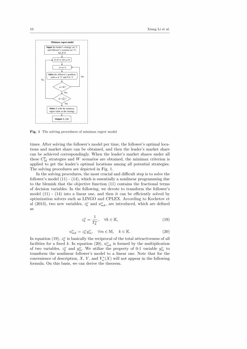
Fig. 1 The solving procedures of minimax regret model

times. After solving the follower’s model per time, the follower’s optimal loca-tions and market share can be obtained, and then the leader’s market sharecan be achieved correspondingly. When the leader’s market shares under allthese Cp

M strategies and W scenarios are obtained, the minimax criterion isapplied to get the leader’s optimal locations among all potential strategies.The solving procedures are depicted in Fig. 1.

In the solving procedures, the most crucial and difficult step is to solve thefollower’s model (11) - (14), which is essentially a nonlinear programming dueto the blemish that the objective function (11) contains the fractional termsof decision variables. In the following, we devote to transform the follower’smodel (11) - (14) into a linear one, and then it can be efficiently solved byoptimization solvers such as LINGO and CPLEX. According to Kochetov etal (2013), two new variables, zωk and uωmk, are introduced, which are definedas

zωk =1

Tωk

, ∀k ∈ K, (19)

uωmk = zωk yωm, ∀m ∈M, k ∈ K. (20)

In equation (19), zωk is basically the reciprocal of the total attractiveness of allfacilities for a fixed k. In equation (20), uωmk is formed by the multiplicationof two variables, zωk and yωm. We utilize the property of 0-1 variable yωm totransform the nonlinear follower’s model to a linear one. Note that for theconvenience of description, X, Y , and Y ∗ω (X) will not appear in the followingformula. On this basis, we can derive the theorem.


Theorem 1 For each ω ∈ W, the follower’s model (11) - (14) is equivalentto the following linear form

max∑k∈K

∑n∈Nf

bkankzωk +

∑k∈K

∑m∈M

bkafmku

ωmk (21)

s. t. (12)− (14) and∑n∈Nf

bkankzωk +

∑m∈M

bkafmku

ωmk + bkz

ωkLk ≤ bk, ∀k ∈ K, (22)

0 ≤ uωmk ≤ yωm,∀m ∈M, k ∈ K, (23)

uωmk ≤ zωk ≤ uωmk + S(1− yωm),∀m ∈M, k ∈ K. (24)

In the above linear equivalent form, the decision variables are yωm, zωk and uωmk.Note that S is a large enough constant in the constraint (24).

Proof For each k ∈ K and ω ∈ W, a constraint should be added to fulfillequation (19), that is,

zωk ≤ 1/Tωk ,

if both sides of the inequality are multiplied by bkTωk , we have

bkzωk T

ωk ≤ bk,

because Tωk = Fω

k + Lk, we get

bkzωk F

ωk + bkz

ωkLk ≤ bk.

The first term is equal to∑

n∈Nf

bkankzωk +

∑m∈M

bkafmku

ωmk, then we get the linear

constraint (22).Constraints (23) and (24) are to fulfill equation (20), in which we utilize

the property of 0-1 variable yωm. When yωm = 0, for each m ∈ M, k ∈ K andω ∈W, equation (20) turns to

uωmk = 0,

which is restricted by constraint (23). For constraint (24), as yωm = 0, it turnsto

uωmk ≤ zωk ≤ uωmk + S,

which is always satisfies.Similarly, when yωm = 1, for each m ∈M, k ∈ K and ω ∈W, equation (20)

turns to

uωmk = zωk ,

which is restricted by constraint (24), while constraint (23) always satisfies.Note that when yωm = 1, zωk ≤ yωm is a constantly established inequality because

12 Xiang Li et al.

zωk =1∑

n∈Nank +

∑m∈M

almkxm +∑

m∈Mafmky

ωm

≤ 1 = yωm,

then we have

0 ≤ uωmk = zωk ≤ yωm,

which means constricts (23) and (24) do not conflict with each other. Then nomatter what the value of yωm, equation (20) is always fulfilled. On this basis,constraints (22) - (24) ensure that equations (19) - (20) are valid.

As for the objective function (21), it is equivalent to (11) because∑k∈K

∑n∈Nf

bkankzωk +

∑k∈K

∑m∈M

bkafmku

ωmk

=∑k∈K

bk

∑n∈Nf

ank +∑m∈M

afmkyωm

zωk

=∑k∈K

bkFωk z

ωk

=∑k∈K

bkFωk

Tωk

.

In the above equation, both∑k∈K

∑n∈Nf

bkankzωk +

∑k∈K

∑m∈M

bkafmku

ωmk and

∑k∈K

bkFω

k

Tωk

represent the follower’s market share, and we devote to maximize it.As a result, follower’s problem (21) - (24) is a linear equivalent form to

(11) - (14). By the transformation, part optimal solution of the linear model(yωm) is the optimal solution to (11) - (14). The proof is completed.

4 Numerical experiments

In this section, numerical experiments are conducted to verify the validity ofthe proposed model and test the efficiency of linearization. In order to furtherexplain the necessity of our hypothesis about the number of follower’s newfacility is unknown or with unknown probability distribution, comparisonswith two different location models are provided to show the advantages of theproposed model.

4.1 An illustration of minimax regert model

We consider an instance with 16 demand points and 5 existing facilities in themarket, as shown in Fig. 2. Among the 5 existing facilities, 3 of them belong tothe leader whose locations are (3,2), (4,3) and (1,4), and the other 2 of them


Fig. 2 The locations of the leader’s and the follower’s existing facilities

belong to the follower whose locations are (3,1) and (3,3). The leader aimsto open 2 new facilities knowing that the follower will open some facilitiesafter his action. However, he does not know the exact number of follower’sfacilities, but knows the maximum number is 4, i.e., the follower may open 1,2, 3 or 4 new facilities. New facilities can not be opened in demand points thatare already occupied by existing facilities. Therefore, the number of candidatelocations for both leader’s and follower’s new facilities is 11. The buying powerat each demand point is randomly generated from the range of 1-10 and we setthe unit of buying power as million yuan. The buying power and coordinatesof demand points are stated in Table 2. Quality values are also given randomlyin the range of 1-5 for new and existing leader’s and follower’s facilities, whichcan be seen in Table 3.

Table 2 Coordinate and buying power of each demand point

Demand point 1 2 3 4 5 6 7 8Coordinate (1,1) (1,2) (1,3) (1,4) (2,1) (2,2) (2,3) (2,4)

Buying power 9 2 2 5 10 4 6 3

Demand point 9 10 11 12 13 14 15 16Coordinate (3,1) (3,2) (3,3) (3,4) (4,1) (4,2) (4,3) (4,4)

Buying power 8 3 6 7 9 8 6 2

According to the solving procedures in Section 3, for each given strategy ofthe leader, we solve the follower’s model firstly. Then the leader’s market sharecan be obtained in each scenario. There are totally C2

11 = 55 potential choicesfor the leader to choose 2 locations among 11 demand points as his strategy,

14 Xiang Li et al.

Table 3 The quality levels for different demand points

QualityLeader Follower

Existing New Existing NewDemand point (3,2) (4,3) (1,4) (3,1) (3,3)

1 4 1 5 1 5 4 32 4 4 2 4 4 1 53 4 1 2 2 1 1 14 5 4 2 3 5 1 35 3 2 4 1 4 1 16 3 3 4 4 4 4 57 2 4 4 2 1 1 18 3 5 2 4 3 2 49 4 2 3 4 4 5 510 5 3 1 4 1 2 511 5 2 5 3 2 5 112 2 1 2 1 4 3 213 2 5 3 2 3 5 214 2 4 4 5 2 3 515 1 1 3 1 4 5 316 1 3 3 5 1 2 5

Table 4 Potential strategies of the leader

Strategy Coordinates Strategy Coordinates Strategy Coordinates1 (1,1),(2,1) 20 (4,1),(1,2) 39 (2,2),(3,4)2 (1,1),(4,1) 21 (4,1),(2,2) 40 (2,2),(4,4)3 (1,1),(1,2) 22 (4,1),(4,2) 41 (4,2),(1,3)4 (1,1),(2,2) 23 (4,1),(1,3) 42 (4,2),(2,3)5 (1,1),(4,2) 24 (4,1),(2,3) 43 (4,2),(2,4)6 (1,1),(1,3) 25 (4,1),(2,4) 44 (4,2),(3,4)7 (1,1),(2,3) 26 (4,1),(3,4) 45 (4,2),(4,4)8 (1,1),(2,4) 27 (4,1),(4,4) 46 (1,3),(2,3)9 (1,1),(3,4) 28 (1,2),(2,2) 47 (1,3),(2,4)10 (1,1),(4,4) 29 (1,2),(4,2) 48 (1,3),(3,4)11 (2,1),(4,1) 30 (1,2),(1,3) 49 (1,3),(4,4)12 (2,1),(1,2) 31 (1,2),(2,3) 50 (2,3),(2,4)13 (2,1),(2,2) 32 (1,2),(2,4) 51 (2,3),(3,4)14 (2,1),(4,2) 33 (1,2),(3,4) 52 (2,3),(4,4)15 (2,1),(1,3) 34 (1,2),(4,4) 53 (2,4),(3,4)16 (2,1),(2,3) 35 (2,2),(4,2) 54 (2,4),(4,4)17 (2,1),(2,4) 36 (2,2),(1,3) 55 (3,4),(4,4)18 (2,1),(3,4) 37 (2,2),(2,3)19 (2,1),(4,4) 38 (2,2),(2,4)

and scenario 1,2,3,4 in the following tables represent that the follower opens1,2,3,4 facilities, respectively. The coordinates of strategy 1 - 55 for the leaderare listed in Table 4. For example, if the leader chooses strategy 1, i.e., (1,1) and(2,1) to open two new facilities, the follower’s problem is solved in candidatelocations for different scenarios. For scenario 1 (the follower opens one newfacility), the leader’s maximum market share is 53.23 million yuan, while forscenario 2 (the follower opens two new facilities), the leader’s maximum marketshare is 45.55 million yuan. Similarly, the market shares are 41.67 million yuan


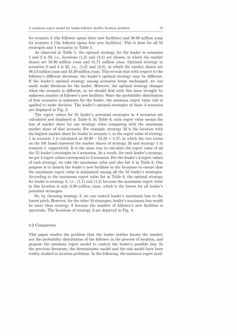
for scenario 3 (the follower opens three new facilities) and 38.60 million yuanfor scenario 4 (the follower opens four new facilities). This is done for all 55strategies and 4 scenarios in Table 5.

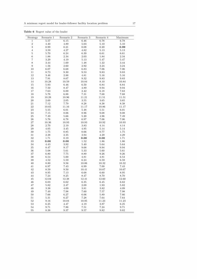
As observed in Table 5, the optimal strategy for the leader in scenarios1 and 2 is 33, i.e., locations (1,2) and (3,4) are chosen, in which the marketshares are 58.80 million yuan and 51.71 million yuan. Optimal strategy inscenarios 3 and 4 is 32, i.e., (1,2) and (2,4), in which the market shares are48.13 million yuan and 45.39 million yuan. This reveals that with respect to thefollower’s different decisions, the leader’s optimal strategy may be different.If the leader’s optimal strategy among scenarios keeps unchanged, we caneasily make decisions for the leader. However, the optimal strategy changeswhen the scenario is different, so we should deal with this issue brought byunknown number of follower’s new facilities. Since the probability distributionof four scenarios is unknown for the leader, the minimax regret value rule isapplied to make decision. The leader’s optimal strategies of these 4 scenariosare displayed in Fig. 3.

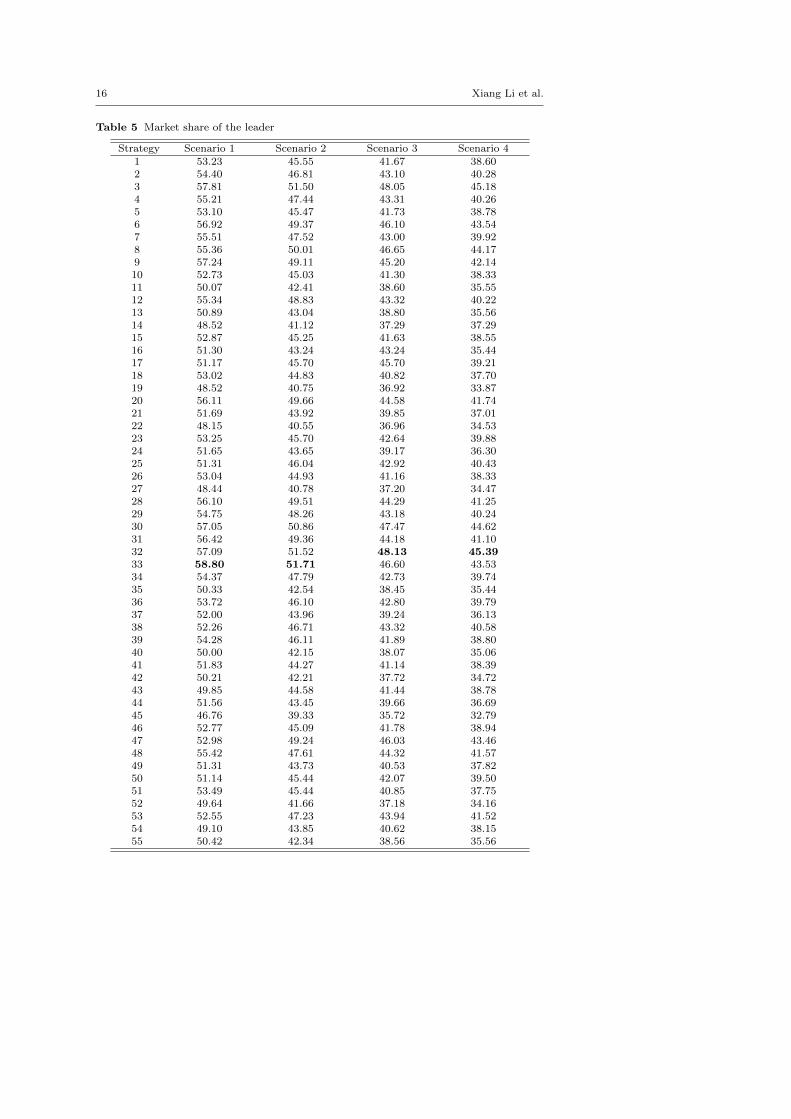
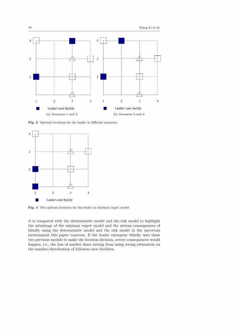
The regret values for 55 leader’s potential strategies in 4 scenarios arecalculated and displayed in Table 6. In Table 6, each regret value means theloss of market share for one strategy when comparing with the maximummarket share of that scenario. For example, strategy 33 is the location withthe highest market share for leader in scenario 1, so the regret value of strategy1 in scenario 1 is calculated as 58.80 − 53.23 = 5.57, in which the two termson the left hand represent the market shares of strategy 33 and strategy 1 inscenario 1, respectively. It is the same way to calculate the regret value of allthe 55 leader’s strategies in 4 scenarios. As a result, for each leader’s strategy,we get 4 regret values correspond to 4 scenarios. For the leader’s 4 regret valuesof each strategy, we take the maximum value and also list it in Table 6. Ourpurpose is to launch the leader’s new facilities in the locations to ensure thatthe maximum regret value is minimized among all the 55 leader’s strategies.According to the maximum regret value list in Table 6, the optimal strategyfor leader is strategy 3, i.e., (1,1) and (1,2) because the maximum regret valuein this location is only 0.99 million yuan, which is the lowest for all leader’spotential strategies.

So, by choosing strategy 3, we can control leader’s maximum loss to thelowest pitch. However, for the other 54 strategies, leader’s maximum loss wouldbe more than strategy 3 because the number of follower’s new facilities isuncertain. The locations of strategy 3 are depicted in Fig. 4.

4.2 Comparison

This paper studies the problem that the leader neither knows the numbernor the probability distribution of the follower in the process of location, andpropose the minimax regret model to control the leader’s possible loss. Inthe previous literature, the deterministic model and the risk model have beenwidely studied in location problems. In the following, the minimax regret mod-

16 Xiang Li et al.

Table 5 Market share of the leader

Strategy Scenario 1 Scenario 2 Scenario 3 Scenario 41 53.23 45.55 41.67 38.602 54.40 46.81 43.10 40.283 57.81 51.50 48.05 45.184 55.21 47.44 43.31 40.265 53.10 45.47 41.73 38.786 56.92 49.37 46.10 43.547 55.51 47.52 43.00 39.928 55.36 50.01 46.65 44.179 57.24 49.11 45.20 42.1410 52.73 45.03 41.30 38.3311 50.07 42.41 38.60 35.5512 55.34 48.83 43.32 40.2213 50.89 43.04 38.80 35.5614 48.52 41.12 37.29 37.2915 52.87 45.25 41.63 38.5516 51.30 43.24 43.24 35.4417 51.17 45.70 45.70 39.2118 53.02 44.83 40.82 37.7019 48.52 40.75 36.92 33.8720 56.11 49.66 44.58 41.7421 51.69 43.92 39.85 37.0122 48.15 40.55 36.96 34.5323 53.25 45.70 42.64 39.8824 51.65 43.65 39.17 36.3025 51.31 46.04 42.92 40.4326 53.04 44.93 41.16 38.3327 48.44 40.78 37.20 34.4728 56.10 49.51 44.29 41.2529 54.75 48.26 43.18 40.2430 57.05 50.86 47.47 44.6231 56.42 49.36 44.18 41.1032 57.09 51.52 48.13 45.3933 58.80 51.71 46.60 43.5334 54.37 47.79 42.73 39.7435 50.33 42.54 38.45 35.4436 53.72 46.10 42.80 39.7937 52.00 43.96 39.24 36.1338 52.26 46.71 43.32 40.5839 54.28 46.11 41.89 38.8040 50.00 42.15 38.07 35.0641 51.83 44.27 41.14 38.3942 50.21 42.21 37.72 34.7243 49.85 44.58 41.44 38.7844 51.56 43.45 39.66 36.6945 46.76 39.33 35.72 32.7946 52.77 45.09 41.78 38.9447 52.98 49.24 46.03 43.4648 55.42 47.61 44.32 41.5749 51.31 43.73 40.53 37.8250 51.14 45.44 42.07 39.5051 53.49 45.44 40.85 37.7552 49.64 41.66 37.18 34.1653 52.55 47.23 43.94 41.5254 49.10 43.85 40.62 38.1555 50.42 42.34 38.56 35.56


Table 6 Regret value of the leader

Strategy Scenario 1 Scenario 2 Scenario 3 Scenario 4 Maximum1 5.57 6.15 6.46 6.78 6.782 4.40 4.89 5.03 5.10 5.103 0.99 0.21 0.08 0.20 0.994 3.59 4.27 4.82 5.13 5.135 5.70 6.24 6.39 6.61 6.616 1.88 2.34 2.03 1.84 2.347 3.29 4.19 5.13 5.47 5.478 3.44 1.69 1.48 1.22 3.449 1.56 2.60 2.92 3.24 3.2410 6.07 6.68 6.83 7.06 7.0611 8.73 9.30 9.53 9.83 9.8312 3.46 2.88 4.81 5.16 5.1613 7.91 8.67 9.32 9.83 9.8314 10.28 10.59 10.84 8.10 10.8415 5.93 6.46 6.50 6.84 6.8416 7.50 8.47 4.89 9.94 9.9417 7.63 6.00 2.42 6.18 7.6318 5.78 6.88 7.31 7.68 7.6819 10.28 10.96 11.21 11.51 11.5120 2.69 2.05 3.55 3.65 3.6521 7.12 7.79 8.28 8.38 8.3822 10.65 11.16 11.17 10.86 11.1723 5.55 6.01 5.48 5.51 6.0124 7.15 8.06 8.96 9.08 9.0825 7.49 5.66 5.20 4.96 7.4926 5.76 6.78 6.97 7.06 7.0627 10.36 10.93 10.93 10.92 10.9328 2.70 2.19 3.83 4.14 4.1429 4.05 3.45 4.95 5.14 5.1430 1.75 0.85 0.66 0.77 1.7531 2.38 2.35 3.94 4.29 4.2932 1.71 0.19 0.00 0.00 1.7133 0.00 0.00 1.52 1.86 1.8634 4.43 3.92 5.40 5.64 5.6435 8.47 9.17 9.68 9.94 9.9436 5.08 5.61 5.33 5.60 5.6137 6.80 7.75 8.89 9.26 9.2638 6.54 5.00 4.81 4.81 6.5439 4.52 5.59 6.24 6.59 6.5940 8.80 9.56 10.06 10.32 10.3241 6.97 7.43 6.99 7.00 7.4342 8.59 9.50 10.41 10.67 10.6743 8.95 7.13 6.68 6.60 8.9544 7.24 8.25 8.47 8.70 8.7045 12.04 12.38 12.41 12.60 12.6046 6.03 6.62 6.35 6.45 6.6247 5.82 2.47 2.09 1.93 5.8248 3.38 4.09 3.81 3.82 4.0949 7.49 7.98 7.60 7.57 7.9850 7.66 6.27 6.06 5.89 7.6651 5.31 6.27 7.28 7.64 7.6452 9.16 10.04 10.95 11.23 11.2353 6.25 4.47 4.19 3.87 6.2554 9.71 7.86 7.51 7.24 9.7155 8.38 9.37 9.57 9.82 9.82

18 Xiang Li et al.

(a) Scenarios 1 and 2 (b) Scenarios 3 and 4

Fig. 3 Optimal locations for the leader in different scenarios

Fig. 4 The optimal locations for the leader in minimax regret model

el is compared with the deterministic model and the risk model to highlightthe advantage of the minimax regret model and the serious consequences ofblindly using the deterministic model and the risk model in the uncertainenvironment this paper concerns. If the leader enterprise blindly uses thesetwo previous models to make the location decision, severe consequences wouldhappen, i.e., the loss of market share arising from using wrong estimation onthe number/distribution of followers new facilities.


4.2.1 Comparison with deterministic model

Starting with Hakimi’s (1983) famous paper on leader-follower problem, mostresearchers considered accurate number of follower’s new facilities, (See Saiz etal., 2009; Kochetov et al., 2013; Gentile et al., 2018). For simplicity, we namethis kind model as deterministic model, in which the leader is going to open pnew facilities and he knows r new facilities will be opened by the follower.

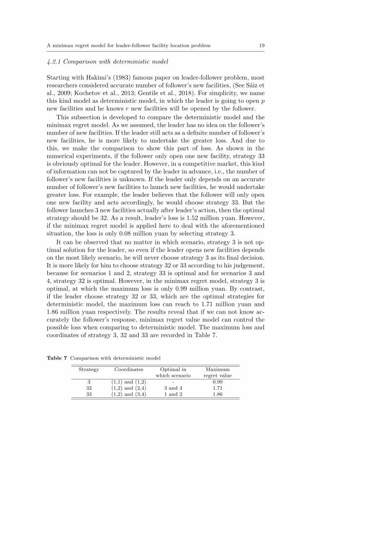
This subsection is developed to compare the deterministic model and theminimax regret model. As we assumed, the leader has no idea on the follower’snumber of new facilities. If the leader still acts as a definite number of follower’snew facilities, he is more likely to undertake the greater loss. And due tothis, we make the comparison to show this part of loss. As shown in thenumerical experiments, if the follower only open one new facility, strategy 33is obviously optimal for the leader. However, in a competitive market, this kindof information can not be captured by the leader in advance, i.e., the number offollower’s new facilities is unknown. If the leader only depends on an accuratenumber of follower’s new facilities to launch new facilities, he would undertakegreater loss. For example, the leader believes that the follower will only openone new facility and acts accordingly, he would choose strategy 33. But thefollower launches 3 new facilities actually after leader’s action, then the optimalstrategy should be 32. As a result, leader’s loss is 1.52 million yuan. However,if the minimax regret model is applied here to deal with the aforementionedsituation, the loss is only 0.08 million yuan by selecting strategy 3.

It can be observed that no matter in which scenario, strategy 3 is not op-timal solution for the leader, so even if the leader opens new facilities dependson the most likely scenario, he will never choose strategy 3 as its final decision.It is more likely for him to choose strategy 32 or 33 according to his judgement,because for scenarios 1 and 2, strategy 33 is optimal and for scenarios 3 and4, strategy 32 is optimal. However, in the minimax regret model, strategy 3 isoptimal, at which the maximum loss is only 0.99 million yuan. By contrast,if the leader choose strategy 32 or 33, which are the optimal strategies fordeterministic model, the maximum loss can reach to 1.71 million yuan and1.86 million yuan respectively. The results reveal that if we can not know ac-curately the follower’s response, minimax regret value model can control thepossible loss when comparing to deterministic model. The maximum loss andcoordinates of strategy 3, 32 and 33 are recorded in Table 7.

Table 7 Comparison with deterministic model

Strategy Coordinates Optimal inwhich scenario

Maximumregret value

3 (1,1) and (1,2) - 0.9932 (1,2) and (2,4) 3 and 4 1.7133 (1,2) and (3,4) 1 and 2 1.86

20 Xiang Li et al.

4.2.2 Comparison with risk model

In Ashtiani et al. (2013), the follower is assumed to open 1, 2,..., pW newfacilities with the probability of P1, P2...PW . The leader’s objective functionis formulated as ‘Expected Value - λ · Variance’

max∑ω∈W

∑k∈K

PωbkLk

Tωk

− λ∑ω∈W

Pω

(∑k∈K

bkLk

Tωk

− Pω

∑k∈K

bkLk

Tωk

)2

.

This objective function maximizes the expected value of leader’s market shareand minimizes the deviation degree between the expected value and the scenar-ios’ optimal solutions simultaneously. In the objective function, λ is a weightcoefficient which measures the importance of variance. The rest of notationshave the same meaning with our proposed minimax regret model.

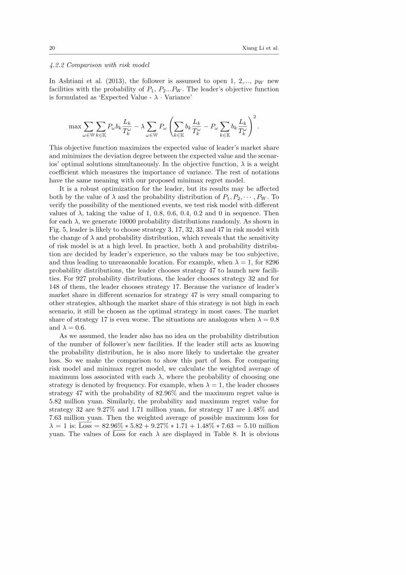
It is a robust optimization for the leader, but its results may be affectedboth by the value of λ and the probability distribution of P1, P2, · · · , PW . Toverify the possibility of the mentioned events, we test risk model with differentvalues of λ, taking the value of 1, 0.8, 0.6, 0.4, 0.2 and 0 in sequence. Thenfor each λ, we generate 10000 probability distributions randomly. As shown inFig. 5, leader is likely to choose strategy 3, 17, 32, 33 and 47 in risk model withthe change of λ and probability distribution, which reveals that the sensitivityof risk model is at a high level. In practice, both λ and probability distribu-tion are decided by leader’s experience, so the values may be too subjective,and thus leading to unreasonable location. For example, when λ = 1, for 8296probability distributions, the leader chooses strategy 47 to launch new facili-ties. For 927 probability distributions, the leader chooses strategy 32 and for148 of them, the leader chooses strategy 17. Because the variance of leader’smarket share in different scenarios for strategy 47 is very small comparing toother strategies, although the market share of this strategy is not high in eachscenario, it still be chosen as the optimal strategy in most cases. The marketshare of strategy 17 is even worse. The situations are analogous when λ = 0.8and λ = 0.6.

As we assumed, the leader also has no idea on the probability distributionof the number of follower’s new facilities. If the leader still acts as knowingthe probability distribution, he is also more likely to undertake the greaterloss. So we make the comparison to show this part of loss. For comparingrisk model and minimax regret model, we calculate the weighted average ofmaximum loss associated with each λ, where the probability of choosing onestrategy is denoted by frequency. For example, when λ = 1, the leader choosesstrategy 47 with the probability of 82.96% and the maximum regret value is5.82 million yuan. Similarly, the probability and maximum regret value forstrategy 32 are 9.27% and 1.71 million yuan, for strategy 17 are 1.48% and7.63 million yuan. Then the weighted average of possible maximum loss forλ = 1 is: Loss = 82.96% ∗ 5.82 + 9.27% ∗ 1.71 + 1.48% ∗ 7.63 = 5.10 millionyuan. The values of Loss for each λ are displayed in Table 8. It is obvious


148

927

8296

Strategy 17 Strategy 32 Strategy 47

92

1332

8577


67

2332

7612


1 16

6671

3312

Strategy 3 Strategy 17Strategy 32 Strategy 33

16

9982

2


7016

1991

993


= 0.8 = 1 = 0.6

= 0.4 = 0.2 = 0

Fig. 5 The results of risk model with different λ

that Loss for all λ in risk model are higher than the possible maximum lossin minimax regret model. The maximum loss is only 0.99 million yuan whenminimax regret model is applied, but the values of Loss in risk model are5.10 million yuan, 5.29 million yuan, 4.88 million yuan, 3.08 million yuan,1.71 million yuan and 1.07 million yuan, respectively. Even if that we do notconsider the variance, the minimax regret model can still reduce the regretvalue from 1.07 million yuan to 0.99 million yuan, and the reduction is due tothe wrong estimation on probability distributions.

All in all, when minimax regret value criterion is applied in leader’s deci-sion, more stable and less risk locations can be obtained. At the same time,there is no need to assume that the information of the number or the probabil-ity distribution of follower’s new facilities is known by the leader in advance,which may be more practical in reality.

Table 8 Comparison with risk model

Risk model λ=1 λ=0.8 λ=0.6 λ=0.4 λ=0.2 λ=0 Minimax regret model

Loss 5.10 5.29 4.88 3.08 1.71 1.07 0.99

4.3 Test the efficiency of linearization

In the solving procedures, we transform the follower’s nonlinear model (11)- (14) into a linear one. In this subsection, we use ten instances of differentscales to test the efficiency of linearization. For each instance, the numbers of

22 Xiang Li et al.

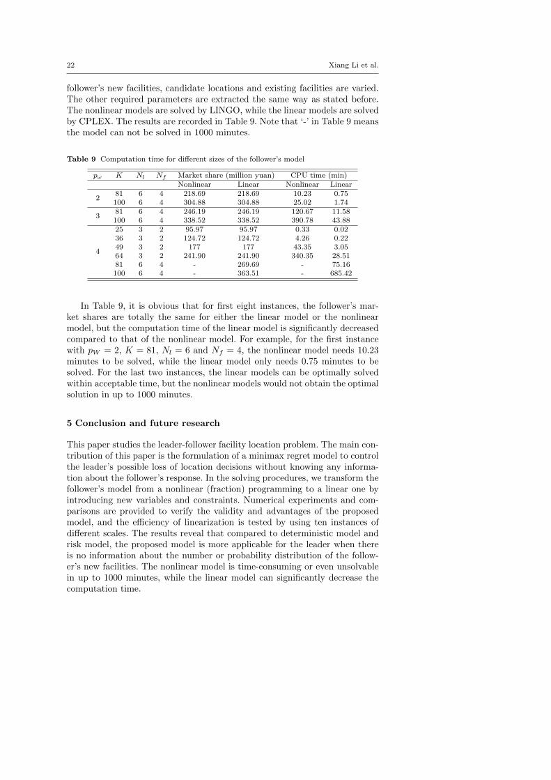
follower’s new facilities, candidate locations and existing facilities are varied.The other required parameters are extracted the same way as stated before.The nonlinear models are solved by LINGO, while the linear models are solvedby CPLEX. The results are recorded in Table 9. Note that ‘-’ in Table 9 meansthe model can not be solved in 1000 minutes.

Table 9 Computation time for different sizes of the follower’s model

pω K Nl Nf Market share (million yuan) CPU time (min)Nonlinear Linear Nonlinear Linear

281 6 4 218.69 218.69 10.23 0.75100 6 4 304.88 304.88 25.02 1.74

381 6 4 246.19 246.19 120.67 11.58100 6 4 338.52 338.52 390.78 43.88

4

25 3 2 95.97 95.97 0.33 0.0236 3 2 124.72 124.72 4.26 0.2249 3 2 177 177 43.35 3.0564 3 2 241.90 241.90 340.35 28.5181 6 4 - 269.69 - 75.16100 6 4 - 363.51 - 685.42

In Table 9, it is obvious that for first eight instances, the follower’s mar-ket shares are totally the same for either the linear model or the nonlinearmodel, but the computation time of the linear model is significantly decreasedcompared to that of the nonlinear model. For example, for the first instancewith pW = 2, K = 81, Nl = 6 and Nf = 4, the nonlinear model needs 10.23minutes to be solved, while the linear model only needs 0.75 minutes to besolved. For the last two instances, the linear models can be optimally solvedwithin acceptable time, but the nonlinear models would not obtain the optimalsolution in up to 1000 minutes.

5 Conclusion and future research

This paper studies the leader-follower facility location problem. The main con-tribution of this paper is the formulation of a minimax regret model to controlthe leader’s possible loss of location decisions without knowing any informa-tion about the follower’s response. In the solving procedures, we transform thefollower’s model from a nonlinear (fraction) programming to a linear one byintroducing new variables and constraints. Numerical experiments and com-parisons are provided to verify the validity and advantages of the proposedmodel, and the efficiency of linearization is tested by using ten instances ofdifferent scales. The results reveal that compared to deterministic model andrisk model, the proposed model is more applicable for the leader when thereis no information about the number or probability distribution of the follow-er’s new facilities. The nonlinear model is time-consuming or even unsolvablein up to 1000 minutes, while the linear model can significantly decrease thecomputation time.


For the future research, we can consider the take-out shops. Goods can bedelivered so the delivery cost rather than the distance would be one influencefactor of the facility’s attractiveness. Also, with the development of deliveryindustry, goods are able to be delivered to some faraway customers, so it isnecessary to develop some efficient meta-heuristic algorithms to solve large-scale problems. In addition, we can also consider the elastic demand for eachdemand point. For example, the buying power of demand points will rise withthe increasing of new facilities, then the market situation for both leader andfollower will be more complex.

Acknowledgements This work was supported by National Natural Science Foundationof China (Grant No. 71722007) and “the Fundamental Research Funds for the CentralUniversities (XK1802-5)”.

Conflict of interest

The authors declare that they have no conflict of interest.

References

1. Aboolian, R., Berman, O., & Krass, D. (2007). Competitive facility location and designproblem. European Journal of Operational Research, 182(1), 40-62.

2. Ahmadi-Javid, A., Seyedi, P., & Syam, S. S. (2016). A survey of healthcare facilitylocation. Computers & Operations Research, 79, 223-263.

3. Ashtiani, M, G., Makui, A., & Ramezanian, R. (2013). A robust model for a leader-follower competitive facility location problem in a discrete space. Applied MathematicalModelling, 37(1-2), 62-71.

4. Dilek, H., Karaer, O., & Nadar, E. (2017). Retail location competition under carbonpenalty. European Journal of Operational Research, 269(1), 146-158.

5. Drezner, T., & Drezner, Z.(1998). Facility location in anticipation of future competition.Location Science, 6(1-4), 155-173.

6. Drezner, T., Drezner, Z., & Kalczynski, P. (2015). A leader-follower model for discretecompetitive facility location. Computers & Operations Research, 64, 51-59.

7. Farahani, R. Z., Fallah, S., Ruiz, R., Hosseini, S., & Asgari, N. (2019). OR models inurban service facility location: A critical review of applications and future developments,European Journal of Operational Research, 276 (1), 1-27.

8. Fernandez, J., G.-Toth, B., Redondo, J. L., Ortigosa, P. M., & Arrondo, A. G.(2017). A planar single-facility competitive location and design problem under the multi-deterministic choice rule. Computers & Operations Research, 78, 305-315.

9. Fernandez, J., G.-Toth, B., Redondo, J. L., & Ortigosa, P. M. (2019). The probabilisticcustomers choice rule with a threshold attraction value: Effect on the location of compet-itive facilities in the plane. Computers & Operations Research, 101, 234-249.

10. Fischer, K. (2002). Sequential discrete p-facility models for competitive location plan-ning. Annals of Operations Research, 111(1-4), 253-270.

11. Gentile, J., Pessoa, A. A., Poss, M., & Roboredo, M. C. (2018). Integer programmingformulations for three sequential discrete competitive location problems with foresight.European Journal of Operational Research, 265, 872-881.

12. Hakimi, S. L. (1983). On locating new facilities in a competitive environment. EuropeanJournal of Operational Research, 12(1), 29-35.

13. Hakimi, S, L. (1986). P-Median theorems for competitive locations. Annals of Opera-tions Research, 6(4), 75-98.

24 Xiang Li et al.

14. Hotelling, H. (1929). Stability in competition. The Economic Journal, 39(153), 41.15. Huff, D. L. (1964). Defining and estimating a trading area. Journal of Marketing, 28(3),

34-38.16. Huff, D. L. (1966). A programmed solution for approximating an optimum retail loca-

tion, Land Economics, 42(3), 293-303.17. Kochetov, Y., Kochetova, N., & Plyasunov, A. (2013). A matheuristic for the leader-

follower facility location and design problem. In: Lau, H., Van Hentenryck, P., Raidl,G.(eds.) Proceedings of the 10th Metaheuristics International Conference (MIC2013). pp.32/1-32/3. Singapore.

18. Kress, D., & Pesch, E. (2012). Sequential competitive location on networks. EuropeanJournal of Operational Research, 217(3), 483-499.

19. Kung, L., & Liao, W. (2018). An approximation algorithm for a competitive facilitylocation problem with network effects. European Journal of Operational Research, 267(1),176-186.

20. Lado-Sestayo, R., & Fernandez-Castro. A. S. (2019). The impact of tourist destinationon hotel efficiency: A data envelopment analysis approach. European Journal of Opera-tional Research, 272(2), 674-686.

21. Lopes, R. B., Ferreira, C., & Santos, B. S. (2016). A simple and effective evolutionary al-gorithm for the capacitated location-routing problem. Computers & Operations Research,70, 155-162.

22. Moore, J. T., & Bard, J. F. (1990). The mixed integer linear bilevel programmingproblem. Operations Research, 38(5), 911-921.

23. Perez, M. D. G., & Pelegrın, B, P. (2003). All stackelberg location equilibria in thehotelling’s duopoly model on a tree with parametric prices. Annals of Operations Research,122(1), 177-192.

24. Plastria, F. (2001). Static competitive facility location: An overview of optimisationapproaches. European Journal of Operational Research, 129(3), 461-470.

25. Plastria, F., & Vanhaverbeke, L. (2008). Discrete models for competitive location withforesight. Computers & Operations Research, 35, 683-700.

26. Qi, M., Xia, M., Zhang, Y., & Miao, L. (2017). Competitive facility location problemwith foresight considering service distance limitations. Computers and Industrial Engi-neering, 112, 483-491.

27. Reilly, W. J. (1931). The law of retail gravitation. New York, NY: Knickerbocker Press.28. Saidani, N., Chu, F., & Chen, H. (2012). Competitive facility location and design with

reactions of competitors already in the market. European Journal of Operational Research,219(1), 9-17.

29. Saiz, M. E., Hendrix, E. M. T., Fernandez, J., & Pelegrın, B. (2009). On a branch-and-bound approach for a huff-like stackelberg location problem. OR Spectrum, 31(3),679-705.

30. Sedghi, N., Shavandi, H., & Abouee-Mehrizi, H. (2017). Joint pricing and location de-cisions in a heterogeneous market. European Journal of Operational Research, 261(1),234-246.

31. Serra, D., & Revelle, C. (1994). Market capture by two competitors: The pre-emptivelocation problem. Journal of Regional Science, 34(4), 549-561.

32. Wang, X., & Ouyang, Y. (2013). A continuum approximation approach to competitivefacility location design under facility disruption risks. Transportation Research: Part B:Methodological, 50, 90-103.

33. Weber, A. (1909). Uber den Standort der Industrien. 1. Teil: Reine Theorie des S-tandortes. TUbingen. Translated as: On the location of industries. p. 1929. Chicago, IL:Unversity of Chicago Press.

34. Xia, Y., Chen, B., Jayaraman, V., & Munson, C. L. (2015). Competition and marketsegmentation of the call center service supply chain. European Journal of OperationalResearch, 247(2), 504-514.

35. Zhang, Y., & Atkins, D. (2019). Medical facility network design: User-choice and system-optimal models. European Journal of Operational Research, 273(1), 305-319.

No. 025/2020/POM/DEC A Minimax Regret Model for Leader ...

Documents

Transcript of No. 025/2020/POM/DEC A Minimax Regret Model for Leader ...