A

MMa

b

c

a

ARRA

KeGSESR

1

dumoltfdt

0d

J. Non-Newtonian Fluid Mech. 165 (2010) 1047–1054

Contents lists available at ScienceDirect

Journal of Non-Newtonian Fluid Mechanics

journa l homepage: www.e lsev ier .com/ locate / jnnfm

nisotropy parameter restrictions for the eXtended Pom-Pom model

ichiel G.H.M. Baltussena, Wilco M.H. Verbeetenc, Arjen C.B. Bogaerdsb,artien A. Hulsena, Gerrit W.M. Petersa,∗

Materials Technology1, Faculty of Mechanical Engineering, Eindhoven University of Technology, P.O. Box 513, 5600 MB Eindhoven, The NetherlandsMaterials Technology, Faculty of Biomedical Engineering, Eindhoven University of Technology, P.O. Box 513, 5600 MB Eindhoven, The NetherlandsDepartamento de Ingeniería Civil, Área de Mecánica de los Medios Continuos y Teoría de Estructuras, Universidad de Burgos, Avenida Cantabria s/n, E-09001 Burgos, Spain

r t i c l e i n f o

rticle history:eceived 1 April 2010eceived in revised form 4 May 2010ccepted 10 May 2010

eywords:Xtended Pom-Pom modeliesekus modelhear viscosityxtensional viscosityecond normal stress coefficientestricted anisotropy parameter

a b s t r a c t

A significant step forward in modelling polymer melt rheology has been the introduction of the Pom-Pomconstitutive model of McLeish and Larson [T.C.B. McLeish, R.G. Larson, Molecular constitutive equa-tions for a class of branched polymers: the Pom-Pom polymer, J. Rheol. 42 (1) (1998) 81–110]. Variousmodifications of the Pom-Pom model have been published over the years in order to overcome sev-eral inconveniences of the original model. Amongst those modified models, the eXtended Pom-Pom(XPP) model of Verbeeten et. al. [W.M.H. Verbeeten, G.W.M. Peters, F.P.T. Baaijens, Differential constitu-tive equations for polymer melts: the extended Pom-Pom model, J. Rheol. 45 (4) (2001) 823–843] hasreceived quite some attention. However, the XPP model has been criticized for the generation of mul-tiple and unphysical solutions. This paper deals with two issues. First, in the XPP model, anisotropy isimplemented in a Giesekus-like manner which is known to result in unphysical solutions for non-linearparameter values ˛ ≥ 0.5. Hence, we put forward the conjecture that a similar limitation holds for theXPP model. In the present paper, the limits for the anisotropy parameter are elaborated on and result tobe most restraining at high deformation rates where the backbone tube is oriented and the backbone tubestretch approaches the number of arms q. By restricting the anisotropy parameter to a maximum criticalvalue the XPP model produces only one solution, which is the correct physical rheology. In the second

part we show that, contrary to the results published by Inkson and Phillips [N.J. Inkson, T.N. Phillips,Unphysical phenomena associated with the extended Pom-Pom model in steady flow, J. Non-Newton.Fluid 145 (2–3) (2007) 92–101], for the special case where the anisotropy parameter equals zero, only onephysically relevant solution exists in unaxial extensional. In addition to this physically relevant solution,also solutions exist in the physically unattainable part of the conformation space. However, the existenceof these physically unattainable solutions is not a unique feature of the XPP model but rather general for

pe rh

non-linear differential ty

. Introduction

The processing of polymer materials has a large influence on theimensional, mechanical, and optical properties of the end prod-ct. The complex rheological behaviour typically encountered inacromolecular fluids is an important reason for that influence. In

rder to predict the viscoelastic behaviour of polymer melts, simu-ation tools have been developed, which need constitutive models

hat can adequately model the polymer dynamics. A significant steporward in modelling polymer melt rheology has been the intro-uction of the Pom-Pom constitutive model [7]. This model is ableo quantitatively predict the correct nonlinear behaviour in both

∗ Corresponding author. Tel.: +31 402474840; fax: +31 402447355.E-mail address: G.W.M.Peters@tue.nl (G.W.M. Peters).

1 http://www.mate.tue.nl/.

377-0257/$ – see front matter © 2010 Elsevier B.V. All rights reserved.oi:10.1016/j.jnnfm.2010.05.002

eological equations.© 2010 Elsevier B.V. All rights reserved.

shear and extension simultaneously for branched materials, suchas low density polyethylene melts.

Various modifications of the Pom-Pom model have been pub-lished over the years in order to overcome several inconveniencesof the original model [2,3,8,9,12]. Amongst those modified models,the eXtended Pom-Pom (XPP) model [12] has received quite someattention. This particular model was successfully implemented ina finite element code and was able to satisfactorily predict thebehaviour of a commercial LDPE melt in complex flow geometriesin a quantitative manner [13,14].

Several authors have criticized the XPP model for both mathe-matical defects [3] and unphysical solutions [3,5]. Both seemingly

alarming issues have each their own specific, yet simple solution.On the one hand, the mathematical defects will mostly be criticalin numerical computations in the vicinity of geometric singulari-ties. These can be circumvented by choosing the double-equationversion of the XPP model, referred to as DXPP, as mentioned by

1 tonia

Vttaaptid

tetmasolmattp

lrfpi

2

fla

�

Hstr

c

wbso

c

�

i

f

HtprimwSb

048 M.G.H.M. Baltussen et al. / J. Non-New

erbeeten et al. [12] and Clemeur et al. [3]. On the other hand,he unphysical solutions, such as turning points [3] and bifurca-ion and multiple solutions [3,5], were shown to be related to thenisotropy parameter ˛. This parameter was introduced to producenon-vanishing second normal stress difference. By restricting thisarameter to a maximum critical value, the correct physical solu-ions do exist and will be encountered starting from an admissiblenitial conformation tensor. The restriction still leaves enough free-om to fit the second normal stress difference.

Clemeur et al. [3] propose to use the double-equation version ofhe eXtended Pom-Pom model and setting the anisotropy param-ter ˛ = 0. In this way, they avoid the mathematical defects ofhe single-equation version and by choosing ˛ = 0, bifurcation and

ultiple solutions are also ommited. This unfortunately comest the cost of losing the second normal stress difference. Theyuggest an alternative way of introducing a non-vanishing sec-nd normal stress coefficient by combining both an upper- andower-convected time derivative, similar to Johnson and Segal-

an [6]. However, such a combination of an upper-convectednd lower-convected time derivative does not fit within thehermodynamic framework GENERIC [10], i.e. combinations arehermodynamically not allowed and a purely upper-convected orurely lower-convected time derivative is preferred.

Since the anisotropy parameter in the XPP model is Giesekus-ike and the anisotropy parameter ˛ in the Giesekus model isestricted [11], it is expected that some restrictions are also presentor the ˛-parameter in the XPP model. The objective of the presentaper is to indicate the limits for the ˛-parameter of the XPP model

n order to avoid unphysical and multiple solutions.

. Modelling

To realistically describe the viscoelastic stresses of polymeruids over a broad range of deformation rates, a multi-modepproximation of the extra-stress tensor � is defined as

=M∑

i=1

Gi (ci − I) . (1)

ere M is the total number of different relaxation times, Gi is thehear modulus of the ith relaxation mode, ci is the conformationensor, and I is the unit tensor. The conformation tensor of the ithelaxation mode is defined as

i = 3�2i Si, (2)

ith �i the backbone stretch and Si the orientation tensor of theackbone tube. In the remainder of this paper we will restrict our-elves to a single mode description of the constitutive behavior andmit the subscript i.

For the eXtended Pom-Pom (XPP) model, time evolution of theonformation tensor follows from

b∇c + [f (c) − 2˛] c + ˛c2 + (˛ − 1) I = 0, (3)

n which the function f (c) is given by

(c) = 2r e�(�−1)(

1 − 1�

)+ 1

�2

[1 − ˛ − ˛

3tr(c2 − 2c)

]. (4)

ere �b is the relaxation time of the backbone tube orientation,aken from the linear relaxation spectrum. ˛ is the anisotropyarameter that influences the second normal stress difference,= �b/�s with �s the relaxation time for the tube stretch, while �

s a parameter determining the influence of the surrounding poly-er chains on the backbone tube stretch and is defined as � = 2/q,here q denotes the amount of arms at the end of a backbone.

ince the trace operator acting on the orientation tensor yields 1y definition, the backbone stretch is defined as � =

√tr(c)/3.

n Fluid Mech. 165 (2010) 1047–1054

Eqs. (1)–(4) give the same XPP model as given in Clemeur et al.[3] and Inkson and Phillips [5]. However, instead of being writtenin terms of the orientation tensor S and backbone tube stretch �or extra-stress tensor � , it is written in terms of the conformationtensor c.

A more appropiate equation for the function f (c), consistentwith the thermodynamical framework GENERIC [8,14], reads

f (c) = 2r e�(�−1)(

1 − 1�2

)+ 1

�2

[1 − ˛ − ˛

3tr(c2 − 2c)

]. (5)

Since the introduction of the second normal stress differenceis Giesekus-like by means of the anisotropy parameter ˛, and thatparameter in the Giesekus model is restricted [11], the evolutionequation of the Giesekus conformation tensor is also given for com-parison

�∇c + [1 − 2˛] c + ˛c2 + (˛ − 1) I = 0, (6)

with � the linear relaxation time.

3. Anisotropy parameter restrictions

Our starting point is the limitation on the parameter ˛ in theGiesekus model, 0 ≤ ˛ ≤ (1/2), as suggested by Bird et al. [1] andlater by Schleininger and Weinacht [11], studying the linear sta-bility of Couette flow. The restriction ensures that the Giesekusmodel does not give solutions with a maximum in the shear orelongational stress, leading to unstable, non-physical solutions. Therestriction also ensures that the linear term in Eq. (6) ([1 − 2˛]c),is positive. We put forward the conjecture that a similar limitationholds for the XPP model, but we are not able to give a formal provefor this and maybe this is not even possible. However, all numeri-cal experiments that we have performed as well as all relevant dataobtained from literature support this conjecture. Also a violation ofour proposed limitation on ˛ may lead to the flow condition thatno steady state solution exists beyond some finite value of �2 (seeAppendix A). With this as a starting point and considering the corre-sponding term in the XPP model [f (c) − 2˛]c, the restriction we putforward reads [f (c) − 2˛] ≥ 0. This leads to a positive linear term inthe XPP model. In this way, the maximum anisotropy parameter ˛allowed becomes a function of the other material parameters andthe conformation tensor c, and thus depends on the stretch andorientation.

For low shear and elongational rates, stretch and orientationare limited which implies that f (c) ≈ 1 and the behavior of theXPP model reduces to the behavior of the Giesekus model. How-ever, at high deformation rates, f (c) changes significantly and,for given ratio r and number of arms q, the critical value of ˛becomes a function of the applied deformation rate. Computation-ally, this can be confirmed by computing the values of the functiong(c) = [f (c) − 2˛] for a relevant series of deformation rates and val-ues of ˛. Contours of g = 0, as shown in Fig. 1, reveal the dependenceof the maximum value for ˛ as a function of the applied shear orextensional rate. The figure shows that, for fixed ratio of relaxationtimes r and increasing number of arms q, the minimum allowablevalue for ˛ appears at high shear or elongational rate. In addition, itshows that the minimum allowable value for ˛ is different in shearand uniaxial extension and appears at different deformation rates.

In order to find an expression for the maximum allowable valueof ˛ in general complex flows (denoted by ˛max) we write thefunction g(c) in the following way:

g(c) = 1�2

[2r e�(�−1)(�2 − �) + 1 − ˛(1 + 3�4tr(S2))

]. (7)

The possible values for c (and thus also of � and tr(S2)) of theXPP model lie on a surface in (c1, c2, c3)-space, where (c1, c2, c3)

M.G.H.M. Baltussen et al. / J. Non-Newtonian Fluid Mech. 165 (2010) 1047–1054 1049

Fig. 1. Maximum allowable ˛ as a function of shear rate (left) and strain rate (right) for a single-mode XPP model. q = 2, 5, 10, 25, r = 3.

Fig. 2. Approximation of the maximum allowable ˛ ( ˆ max) in (r, q)-space. Fourregions can be observed, I and III where q ≥ 2 +

√3, II and IV where q < 2 +

√3. In III

as

afofgafuct(˛

Eq. (7) is only a function of � and linear in ˛, from which we easilyfind the value for ˛ for which g = 0 as a function of �:

FX

nd IV, ˆ max is limited by the upper bound 0.5, whereas in I and II the approximationpecified in the second argument of Eq. (10) is used.

re the principal values of c (see Appendix A). In addition, this sur-ace depends on the parameters (r, q, ˛) in the model. The valuef ˛max is the maximum value of ˛ for which g(c) ≥ 0 on the sur-ace in (c1, c2, c3)-space. In Appendix A we have shown that for aiven stretch � the maximum value of tr(S2) is obtained for uni-xial elongational flow. Therefore, it follows from the expressionor g(c) in Eq. (7) that the minimum value for ˛max is obtained inniaxial elongational flow. This means we only have to consider aurve instead of a surface in (c1, c2, c3)-space to find ˛max. Note,

hat in equilibrium we have � = 1 and tr(S2) = (1/3) and from Eq.7) we find g = 1 − 2˛ for this case. This leads to an upper boundmax ≤ (1/2) for any parameter set (r, q).

ig. 3. Relative error (˛max − ˆ max)/˛max. The left graph shows results for the original XPPP model using the same ˆ max as for the XPP model. The blocky behavior comes from th

Fig. 4. Maximum admissible ˛ according to Eqs. (10) and (11) as a function of theamount of arms q and simple guidelines ˛ = 0.1/q and ˛ = 0.3/q with r = 1.

Even though we can restrict the possible values for � and tr(S2)to the curve for uniaxial elongational flow, the expressions are stillcomplicated and finding an analytical solution is difficult. There-fore, we try to find an approximation for ˛max. First we approximatethe uniaxial elongational flow curve by tr(S2) = 1, overpredictingtr(S2). If we denote the maximum allowed value for ˛ using thisapproximation by ˛∗

max, we find ˛∗max < ˛max. By this choice g in

˛∗(�) = 2r e�(�−1)(�2 − �) + 11 + 3�4

, (8)

P model while the right graph shows results for the thermodynamically consistente low amount of grey levels in the colorbar.

1050 M.G.H.M. Baltussen et al. / J. Non-Newtonian Fluid Mech. 165 (2010) 1047–1054

Fig. 5. Contour lines of the function H on a part of the physically attainable cxx, cyy-plane for (G = 1 [Pa], �b = 3 [s], �s = 1 [s], q = 10 [–], ˛ = 0 [–]) and ε = 0.01 [1/s](left)and ε = 0.1 [1/s](right).

F d corrl data g

af˛b

˛

ait

˛

w

�

s2i

ow0a

u

than a guideline for the consistent implementation of the XPP mod-els and one may always resolve the full set of equations for uniaxialextensional flow to determine the “exact” value ˛max.

ig. 6. Contour lines of H on a part of the full cxx, cyy-plane for ε = 0.1 [1/s](left) anine is the negative elongational viscosity. The constitutive data corresponds to the

nd ˛∗max is the minimum of this function over the range � ≥ 1. This

unction is still too complicated to find an analytical expression for∗max. For large values of � the function ˛∗(�) can be approximatedy

∗(�) ≈ 2r e�(�−1)(�2 − �)3�4

= 23

r e�(�−1)(

1�2

− 1�3

), (9)

nd the value for � where the right-hand side is minimal can be eas-ly found by solving a quadratic equation. Based on that, we proposehe following approximate value for ˛max, denoted by ˆ max:

ˆ max = min

(12

,2r e�(�−1)(�2 − �) + 1

1 + 3�4

), (10)

ith � defined by

ˆ =

⎧⎨⎩

1 + q

2for q < 2 +

√3

1 + q +√

(q − 2)2 − 32

for q ≥ 2 +√

3(11)

The second case for � is found by minimizing the right-handide of Eq. (9). Since this would become a complex value for q <+

√3, we use the real part only for that range of q. Note, that we

ncluded the upper-bound for ˛max of (1/2) found earlier.We can now distinguish four regions in (r, q)-space for the value

f ˆ max which are shown in Fig. 2: I and III where q ≥ 2 +√

3, II and IV√

here q < 2 + 3. In III and IV, ˆ max is limited by the upper bound

.5, whereas in I and II the approximation specified in the secondrgument of Eq. (10) is used.

The introduction of the approximation tr(S2) = 1 leads to annderprediction of ˛max. However, the sign of the error intro-

esponding absolute value of the uniaxial elongational viscosity (right). The dashediven in Fig. 5.

duced by � is undetermined. To confirm that the approximationgiven above, and shown in Fig. 2, is actually a conservative one,i.e. ˆ max ≤ ˛max, we consider the relevant part of the (r, q)-spaceand compare ˆ max with the “exact” ˛max using the numerical algo-rithm as used for producing Fig. 1. As has been shown before, ˛max

can be found by considering uniaxial extensional flows only, whichsimplifies the problem of finding the ˆ max significantly.

In the left graph of Fig. 3, the relative error (˛max − ˆ max)/˛max isshown for the original XPP model. It can be observed that this erroris always positive in the entire (r, q)-space and thus the approxima-tion is a conservative one. Also, it can be observed that the largesterror occurs for small r and small q.2 This, however, is never morethan 10% for q ≥ 3 and decreases fast in more relevant regions ofthe (r, q)-space.

For the thermodynamically consistent version of the XPP model,one could argue to follow the same strategy to arrive at an esti-mate ˆ max. Unfortunately, this does not result in a conservativeapproxiation. However, as is shown in the right graph of Fig. 3, theapproximation given by (10) and (11) also provides a conservativeestimate for ˛max for the thermodynamically consistent XPP modelalbeit at the cost of accuracy.

It should be noted that the estimate ˆ max provides nothing more

2 Combinations of low r and low q are not very physical. Typically, r → 1 for largeq-values and r ≥ 3 for q = 2. See [12–14] for a number of illustrative parameterssets.

M.G.H.M. Baltussen et al. / J. Non-Newtonian Fluid Mech. 165 (2010) 1047–1054 1051

F ε = 0.b left) ac rame

tcdficiwv

wts

TN

ig. 7. Contour lines of the corresponding H-function for the linear PTT model andottom graphs show the absolute value of �u for the exponential PTT model (bottomonvective derivative is applied and the value of the single remaining non-linear pa

In previous papers [12–14], a different guideline for choosinghe anisotropy parameter ˛ was given as ˛ = 0.1/q or ˛ = 0.3/q inase no second normal stress difference or second planar viscosityata is available. That simple rule of thumb will generally workne. However, especially for high q and low r it is recommended toheck the admissibility of the ˛-parameter using Eqs. (10) and (11)n order to avoid possible numerical problems. In general, ˛ = 0.1/q

ill not violate the maximum allowable value for q < 45. Fig. 4isually illustrates these statements.

Inkson and Phillips [5] show numerous plots in their paperhere, starting from different initial values, multiple solutions of

he XPP model are found. In all of these plots, also a correct physicalolution is found, with exception of the cases where the anisotropy

able 1on-linear parameters used to calculate bifurcations for the single-mode XPP model with

q ˛ ˆ max Cor

2 0.00 0.5 Yes2 0.10 0.5 Yes2 0.15 0.5 Yes2 1.00 0.5 No

10 0.00 0.1086 Yes10 0.03 0.1086 Yes10 0.10 0.1086 Yes10 1.00 0.1086 No25 0.00 0.0209 Yes25 0.012 0.0209 Yes25 0.10 0.0209 No25 1.00 0.0209 No10 0.03 0.1086 Yes20 unknown 0.0317 No

1[1/s](topleft) and corresponding value of the elongational viscosity (topright). Thend the Giesekus model (bottomright). For all cases G = 1 and � = 3, only the upper

ter is fixed at 0.1. The dashed lines represent the negative elongational viscosities.

parameter ˛ is above its maximum allowable value. Table 1 showsthe cases represented in their paper, the maximum allowable ˛-parameter and if a correct physical solution was found or not.

As can be seen from Table 1, most studied cases do encounter acorrect physical solution, with the exceptions of all cases with ˛ = 1and the q = 25, ˛ = 0.1 combination. This last case is also the casewhere Inkson and Phillips [5] found most problems, amongst othersa positive second normal stress coefficient. Therefore, the unphys-ical solutions found by Inkson and Phillips [5] can be explained by

the choice of an inadmissible ˛-parameter.

Turning points were found in the steady shear viscosity of theXPP model by Clemeur et al. [3], as illustrated by Fig. 1 in theirpaper. It is speculated that this effect is also due to an anisotropy

G = 1, r = 3. ˆ max is calculated according to Eqs. (10) and (11).

rect physical solution f (c) Reference

Eq. (4) [5]Eq. (4) [5]Eq. (4) [5]Eq. (4) [5]Eq. (4) [5]Eq. (4) [5]Eq. (4) [5]Eq. (4) [5]Eq. (4) [5]Eq. (4) [5]Eq. (4) [5]Eq. (4) [5]Eq. (5) [5]Eq. (4) [3]

1 tonia

pi

4

fltsebItr

I

Jwp(o

H

sc

a(eaftomHtf(

wssa

figfld

ab(ac

5

ep

052 M.G.H.M. Baltussen et al. / J. Non-New

arameter ˛ above its limiting value. However, since the value for ˛s not given in the paper, unfortunately, this can not be confirmed.

. Multiple solutions

Inkson and Phillips [5] also find that in uniaxial extensionalows, even for ˛ = 0, multiple solutions exist for low deforma-ion rates. However, we were unable to reproduce these additionalolutions. It is beyond the scope of this article to provide a full math-matical proof of the existence of only a single solution for ˛ = 0ut it can be readily shown that the multiple solutions found by

nkson and Phillips cannot be correct. In terms of the conformationensor, the steady state Eq. (3) in uniaxial extensional flow for ˛ = 0educe to

(cxx, cyy) = cxx

(f (cxx, cyy) − 2�bε

)− 1 = 0, (12)

(cxx, cyy) = cyy

(f (cxx, cyy) + �bε

)− 1 = 0, (13)

ith cxx and cyy the conformation in the extensional and the per-endicular directions respectively and f (cxx, cyy) as defined by Eq.4). If, depending on a fixed value of the deformation rate, the normf the residues (I and J) on the cxx, cyy-plane is defined as

(cxx, cyy) =√

I(cxx, cyy)2 + J(cxx, cyy)2, (14)

olutions of (12) and (13) are found when H(cxx, cyy) = 0. Numeri-ally the function H is easily constructed on a 2-dimensional grid.

For comparison, we take Fig. 10(a) of the paper of Inksonnd Phillips [5] and the material parameters that it representsG = 1 [Pa], �b = 3 [s], �s = 1 [s], q = 10 [–], ˛ = 0 [–]) as a refer-nce. Fig. 5 now shows the contourlines of H in a physicallyllowable part of the cxx, cyy-plane (where c is positive definite)or ε = 0.01 [1/s] and ε = 0.1 [1/s]. For the dataset chosen here,he XPP model obviously predicts only one solution which is thene we may expect. Of course, this does not show yet that thereay not exist other solutions in other parts of the cxx, cyy-plane.owever, for the remainder of the physically attainable part of

he conformation space where tr(c) 3, the function f reduces to≈ 2r exp(�

√tr(c)/3) 1. For the limit of small deformation rates

ε 1) a linear combination of (12) and (13) yields

23

rtr(c) exp

(�

√tr(c)

3

)= 1, (15)

hich, since �b > �s, does not have a solution in the conformationpace outside the region shown in Fig. 5. Therefore only a singleolution is found in the physically attainable conformation spaces opposed to the results given in Inkson and Phillips [5].

Still, as is shown in Fig. 6, at least one additional solution existsor indefinite conformation tensors. This additional solution resultsn a ‘negative elongational viscosity’ which is shown in the rightraph of Fig. 6. The same approach, applied to homogeneous shearow, did not result in any additional (non-physical) solution at loweformation rates.

For uniaxial deformation, the obtained non-physical solutionsre not a unique feature of the XPP model. A similar analysis ofoth the linear and the exponential Phan-Thien Tanner (PTT) modelwithout mixed derivatives) and the Giesekus model shows thatlso for these models solutions exist for non-physical values of theonformation tensor (Fig. 7).

. Conclusions

The restrictions concerning the anisotropy parameter ˛ of theXtended Pom-Pom (XPP) model have been investigated. Thisarameter is responsible for the introduction of a non-zero second

n Fluid Mech. 165 (2010) 1047–1054

normal stress coefficient in shear flows as well as a second planarelongational viscosity in a Giesekus-like manner.

Similar to the Giesekus model [11], we pose that constraintsmay exist for the anisotropy parameter. However, these are muchmore strict for the XPP model than for the Giesekus model. Themaximum admissible value for ˛ depends on the applied flow butit is shown that it is most restrictive in uniaxial elongational. Anestimate for the anisotropy parameter is given by Eqs. (10) and(11). If a too high value for ˛ is chosen, a solution for the XPP modeleither does not exist or is not stable and admissible for large valuesof the deformation rate, similar as for the Giesekus model. BothInkson and Phillips [5] and Clemeur et al. [3] have encounteredsuch incorrect solutions.

Contrary to the results obtained by Inkson and Phillips [5], it isalso shown that for the special case where ˛ equals zero (whichby our definition should be admissible), only one physically rele-vant solution is obtained in unaxial extensional flows. In additionto this physically relevant solution, also solutions can exist in thephysically unattainable part of the conformation space. It is shownthat this is not a characteristic of the XPP model but rather a com-mon feature of non-linear differential type rheological equations.In transient flow problems, it was shown by Hulsen [4] that thesenon-physical solutions can never occur (for admissible values ofthe non-linear parameter) provided that the initial conformationis positive definite. The XPP model also conforms to the conditionsgiven by Hulsen [4] and the additional solution as shown in Fig. 6should not lead to any problems when a time dependent flow prob-lem is considered. However, when the steady state solution of a flowcharacterized by homogeneous elongational deformation is soughtiteratively rather than by time integration (as is customary for thelinear stability analyses of these flows) it is possible to converge tothe physically incorrect solution instead of to the correct one.

Appendix A. The maximum value of tr(S2) for given stretch� in the XPP model

In this appendix we will show that for given stretch � the valueof tr(S2) is is maximal in uniaxial elongational flow, i.e. the highestorientation for given stretch is found in uniaxial elongation.

In the XPP model the following tensor function has been defined

f (c) = f1(�) + 1�2

[1 − ˛ − ˛

3tr(c2 − 2c)], (16)

where c is the conformation tensor, the stretch � =√

tr(c)/3 and

f1(�) =

⎧⎨⎩

2r e�(�−1)

(1 − 1

�

)original model,

2r e�(�−1)

(1 − 1

�2

)thermodynamically consistent model.

(17)

Note, that c is a positive definite tensor and therefore � is alwaysdefined. The function f (c) can be written as follows:

f (c) = f1(�) + 1�2

[1 − ˛ − ˛

3tr(c2 − 2c)

]= f1(�) + 1

�2

[1 − ˛ − ˛

3tr(c2) + 2˛

3tr(c)

]

= f1(�) + 1

�2

[1 − ˛ − ˛

3tr(c2) + 2˛�2

]= f1(�) + 1

�2

[1 − ˛ − ˛

3tr(c2)

]+ 2˛.

(18)

tonian Fluid Mech. 165 (2010) 1047–1054 1053

A

w

S

of

g

�vtflf

�

w

No

I

w

I

I

I

Nt

fi

G

dsofi

iaootsc

a

t

d

Fig. A.1. Contour lines of tr(S2) (thick solid lines) and det(S) (thin solid lines) onan equilateral triangle. Also shown are the lines of uniaxial elongation (dashedlines) with s2 = s3 = (1 − s1)/2, s1 > (1/3) (cyclic). Note, that on the triangle (1/3) ≤tr(S2) < 1, where the lowest value is in the centroid ((1/3), (1/3), (1/3)) and thehighest value in the corners (cannot be reached by the model). Also, on the triangle

M.G.H.M. Baltussen et al. / J. Non-New

nd thus

g(c) = f (c) − 2˛

= f1(�) + 1�2

[1 − ˛ − ˛

3tr(c2)

]= f1(�) + 1

�2

[1 − ˛ − 3˛�4tr(S2)

] (19)

here the orientation tensor S has been defined as

= ctr(c)

= c3�2

. (20)

Note, that tr(S) = 1 and that S is a positive definite tensor. Basedn our approach of Section 3, we propose the following restrictionor existence and stability:

(c) > 0. (21)

For given material parameters (˛, r, �) and specified stretchthe function g(c) is minimal for tr(S2) obtaining the maximum

alue. Next we will show that for steady flow (in a Lagrangian sense)he maximum value of tr(S2) is obtained for uniaxial elongationows. This means we only need to test uniaxial elongation flows

or evaluating the minimum value of g(c).We write the XPP model in the following form

b∇c = h1(c)I + h2(c)c + h3(c)c2 (22)

ith

h1(c) = 1 − ˛h2(c) = −f (c) + 2˛ = −g(c)h3(c) = −˛

ote, that h1 and h2 are constants and h2(c) (like g(c)) is a functionf � and tr(S2).

Following Hulsen [4] we find that

˙3 = I3tr(c−1c) = h1I2 + (3h2 + h3I1)I3 (23)

here the invariants of c are defined by

1 = tr(c) = 3�2 (24)

2 = 12

[I21 − tr(c2)] = 9

2�4[1 − tr(S2)] (25)

3 = det(c) = 27�6 det(S) (26)

ote, that I1 > 0, I2 > 0 and I3 > 0 since c is a positive definiteensor.

Considering only steady solutions (in the Lagrangian sense) wend from Eq. (23) with I3 = 0

(�tr(S2), det(S)) = h1I2 + (3h2 + h3I1)I3 = 0 (27)

escribing a “surface” in solution space for c on which all steadytate solutions can be found. Using (c1, c2, c3), the principal valuesf c, Eq. (27) is a surface in (c1, c2, c3)-space, which consists of therst octant only.

For a given stretch �, i.e. c1 + c2 + c3 = 3�2, the surface G = 0 isntersected by a plane with normal vector (1, 1, 1) and reduces tocurve. Also the intersection of that plane with the solution spacef (c1, c2, c3) (first octant) is a equilateral triangle. The values of cn that triangle are most conveniently described using the orien-ation tensor S = c/(3�2) and its principal values (s1, s2, s3). Since1 + s2 + s3 = 1, the principal values of S represent the barycentricoordinates on the triangle.

2

For a given stretch �, the two remaining invariants are tr(S )nd det(S)

r(S2) = s21 + s2

2 + s23 (28)

et(S) = s1s2s3 (29)

0 < det(S) ≤ (1/27), where the lowest value is on the edges (cannot be reached bythe model) and the highest value is in the centroid.

which are both positive. In Fig. A.1 we have plotted contours oftr(S2) and det(S). Note, that the contours of tr(S2) are concentriccircles with the center of the circles at the centroid of the triangle.The contour values increase with the radius. The contours of det(S)are curves with a 120 degrees rotational symmetry and a mirrorsymmetry with respect to the middle line towards the vertices (theuniaxial elongation lines). The contour values are maximal near thecentroid and minimal near the edges of the triangle. If we start ata point on the uniaxial elongation lines and stay on the circles ofconstant tr(S2) the value of det(S) will always decrease. We will usethis corollory in the following.

The function G in Eq. (27) can be written as follows

G = h4 + h5I3 (30)

where

h4 = h1I2 = (1 − ˛)I2h5 = 3h2 + h3I1 = −3g(c) − ˛I1

We see that for specified � and tr(S2) the coefficients h4 and h5are constant and that h4 > 0 (assuming ˛ < 1) and h5 < 0. Here wehave used that g(c) > 0 because of existence and stability require-ments we have imposed (see Section 3). Since h4 > 0 it is requiredthat h5 < 0 otherwise the curve G = 0 does not exist. If the criteriumg > 0 is violated it is very well possible that h5 can become posi-tive and no solution will exist for the specified stretch �. Note, thatg < 0 corresponds to ˛ > (1/2) in the Giesekus model, denotingthe range for ˛ where stress maxima in shear are observed.

In Fig. A.2 we have plotted a curve G = 0 and a circular contourof tr(S2) that starts from the intersection of G = 0 with the uniaxialelongation line. Note, that on the edges of the triangle we haveG = h4 > 0. Hence the value of G will be positive on the “outside”and negative on the “inside”. It we ‘walk’ along the circle startingfrom the uniaxial elongation line the value of det(S) will decrease(and thus also I3). Since the coefficient h5 is negative in Eq. (30),the value of G will increase (become positive). This means that the

curve G = 0 will be on the inside of the circle. Consequently, thestarting point on the uniaxial elongation line has the maximumvalue for tr(S2).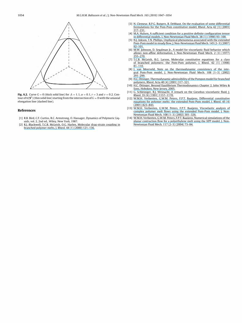

1054 M.G.H.M. Baltussen et al. / J. Non-Newtonia

Fte

R

[

[

[

[13] W.M.H. Verbeeten, G.W.M. Peters, F.P.T. Baaijens, Viscoelastic analysis of

ig. A.2. Curve G = 0 (thick solid line) for � = 1.1, ˛ = 0.1, r = 3 and � = 0.2. Con-our of tr(S2) (thin solid line) starting from the intersection of G = 0 with the uniaxiallongation line (dashed line).

eferences

[1] R.B. Bird, C.F. Curtiss, R.C. Armstrong, O. Hassager, Dynamics of Polymeric Liq-uids, vol. 2, 2nd ed., Wiley, New York, 1987.

[2] R.J. Blackwell, T.C.B. McLeish, O.G. Harlen, Molecular drag-strain coupling inbranched polymer melts, J. Rheol. 44 (1) (2000) 121–136.

[

n Fluid Mech. 165 (2010) 1047–1054

[3] N. Clemeur, R.P.G. Rutgers, B. Debbaut, On the evaluation of some differentialformulations for the Pom-Pom constitutive model, Rheol. Acta 42 (3) (2003)217–231.

[4] M.A. Hulsen, A sufficient condition for a positive definite configuration tensorin differential models, J. Non-Newtonian Fluid Mech. 38 (1) (1990) 93–100.

[5] N.J. Inkson, T.N. Phillips, Unphysical phenomena associated with the extendedPom-Pom model in steady flow, J. Non-Newtonian Fluid Mech. 145 (2–3) (2007)92–101.

[6] M.W. Johnson, D. Segalman Jr., A model for viscoelastic fluid behavior whichallows non-affine deformation, J. Non-Newtonian Fluid Mech. 2 (3) (1977)255–270.

[7] T.C.B. McLeish, R.G. Larson, Molecular constitutive equations for a classof branched polymers: the Pom-Pom polymer, J. Rheol. 42 (1) (1998)81–110.

[8] J. van Meerveld, Note on the thermodynamic consistency of the inte-gral Pom-Pom model, J. Non-Newtonian Fluid Mech. 108 (1–3) (2002)291–299.

[9] H.C. Öttinger, Thermodynamic admissibility of the Pompon model for branchedpolymers, Rheol. Acta 40 (4) (2001) 317–321.

10] H.C. Öttinger, Beyond Equilibrium Thermodynamics Chapter 2, John Wiley &Sons, Hoboken, New Jersey, 2005.

11] G. Schleiniger, R.J. Weinacht, A remark on the Giesekus viscoelastic fluid, J.Rheol. 35 (6) (1991) 1157–1170.

12] W.M.H. Verbeeten, G.W.M. Peters, F.P.T. Baaijens, Differential constitutiveequations for polymer melts: the extended Pom-Pom model, J. Rheol. 45 (4)(2001) 823–843.

complex polymer melt flows using the extended Pom-Pom model, J. Non-Newtonian Fluid Mech. 108 (1–3) (2002) 301–326.

14] W.M.H. Verbeeten, G.W.M. Peters, F.P.T. Baaijens, Numerical simulations of theplanar contraction flow for a polyethylene melt using the XPP model, J. Non-Newtonian Fluid Mech. 117 (2–3) (2004) 73–84.