Minmax regret approach and optimality evaluation in

combinatorial optimization problems with interval and

fuzzy weights

Adam Kasperski

Institute of Industrial Engineering and Management, Wroc law University of Technology,

Wybrzeze Wyspianskiego 27, 50-370 Wroc law, Poland, adam.kasperski@pwr.wroc.pl

Pawe l Zielinski∗

Institute of Mathematics and Computer Science Wroc law University of Technology,

Wybrzeze Wyspianskiego 27, 50-370 Wroc law, Poland, pawel.zielinski@pwr.wroc.pl

Abstract

This paper deals with a general combinatorial optimization problem in whichclosed intervals and fuzzy intervals model uncertain element weights. The notionof a deviation interval is introduced, which allows us to characterize the optimalityand the robustness of solutions and elements. The problem of computing deviationintervals is addressed and some new complexity results in this field are provided.Possibility theory is then applied to generalize a deviation interval and a solutionconcept to fuzzy ones.

Keywords: Minmax regret; Interval; Possibility theory; Combinatorial optimization

1 Introduction

A wide class of deterministic combinatorial optimization problems with a linear objectivefunction consists in finding a feasible solution from a finite set whose total weight is maximalor minimal. Typically, a set of feasible solutions is formed by subsets of a given finite set ofelements E. Every element in E has a nonnegative weight and we seek a feasible solutionwhose total weight is minimal or maximal. An element e ∈ E is called optimal if it is apart of an optimal solution.

In many real-world applications the element weights may be ill-known or uncertain.The simplest form of the uncertainty representation is to specify the element weights as

∗Corresponding author

1

closed intervals. Every precise instantiation of the weights is called a configuration (it isalso called a scenario in the literature). Now a solution (an element) is possibly optimal ifit is optimal for at least one configuration (the event that it will be optimal is possible).Similarly, a solution (an element) is necessarily optimal if it is optimal for all configurations(the event that it will be optimal is sure). The notions of possible and necessary optimalityof solutions and elements have been already introduced in the literature for some particularproblems: in [8, 9, 10, 12, 14] for scheduling problems, in [21] for matroidal problems,in [16, 17, 18] for linear programming, in [19] for shortest path and in [27] for minimumspanning tree. In this paper, we generalize the optimality notions to all combinatorialoptimization problems with interval weights. We show that both possible and necessaryoptimality can be expressed by means of the so-called deviation interval, which providessome additional information under uncertainty. The upper bound of the deviation intervalof a solution is called in the literature a maximal regret and it is a natural criterion forchoosing a solution under the interval representation of uncertainty (see [22]). Namely, inthe minmax regret approach we seek a solution that minimizes the maximal regret andthis approach to combinatorial optimization has been extensively studied in the recentliterature (see, e.g. [2, 3, 5, 6, 19, 20, 24, 27] and [4] for a recent survey).

In this paper, we show some general relationships between the deviation interval, thepossible and necessary optimality and the minmax regret approach. We provide somenew results and we generalize the results known for some particular problems. We alsodiscuss the problem of computing bounds of the deviation interval for a given solutionor an element. In particular, we provide new complexity results for some basic problemssuch as shortest path, minimum assignment and minimum s− t cut. The results obtainedfor the interval-valued case can be generalized so that uncertainty is modeled in a moresophisticated manner. The key idea is to generalize the classical closed interval to a fuzzyone. A fuzzy interval is regarded as a possibility distribution describing the set of more orless plausible values of an element weight. Using possibility theory [11] we can generalizethe notion of the deviation interval to the fuzzy case. From a fuzzy deviation interval,that is a possibility distribution representing a set of plausible values of solution (element)deviations, we can derive the degrees of possible and necessary optimality of a solution (anelement). As in the interval case, we can use an upper bound of the fuzzy deviation intervalto choose a solution. This leads to the concept of a necessary soft optimality, which hasbeen originally proposed in [17, 18] for linear programming problem with a fuzzy objectivefunction. Choosing a best necessarily soft optimal solution is a direct generalization of theminmax regret approach to the fuzzy case.

This paper is organized as follows. In Section 2 we recall a formulation of the deter-ministic combinatorial optimization problem. In Section 3 we discuss the problem withuncertain weights modeled as closed intervals. We introduce the concept of the deviationinterval and we show some various properties of this notion. In particular, we show thatcomputing the lower bound of the deviation interval for a given element is NP-hard forsome basic problems. Section 4 is devoted to a general combinatorial optimization prob-lems with uncertain weights modeled by fuzzy intervals. We show how the notions andresults presented in Section 3 can be naturally generalized to the fuzzy case.

2

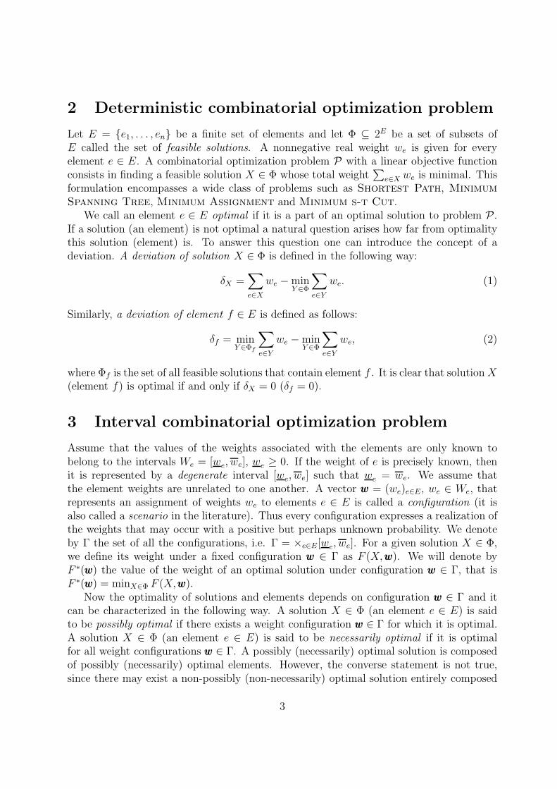
2 Deterministic combinatorial optimization problem

Let E = e1, . . . , en be a finite set of elements and let Φ ⊆ 2E be a set of subsets ofE called the set of feasible solutions. A nonnegative real weight we is given for everyelement e ∈ E. A combinatorial optimization problem P with a linear objective functionconsists in finding a feasible solution X ∈ Φ whose total weight

∑e∈X we is minimal. This

formulation encompasses a wide class of problems such as Shortest Path, Minimum

Spanning Tree, Minimum Assignment and Minimum s-t Cut.We call an element e ∈ E optimal if it is a part of an optimal solution to problem P.

If a solution (an element) is not optimal a natural question arises how far from optimalitythis solution (element) is. To answer this question one can introduce the concept of adeviation. A deviation of solution X ∈ Φ is defined in the following way:

δX =∑

e∈X

we − minY ∈Φ

∑

e∈Y

we. (1)

Similarly, a deviation of element f ∈ E is defined as follows:

δf = minY ∈Φf

∑

e∈Y

we − minY ∈Φ

∑

e∈Y

we, (2)

where Φf is the set of all feasible solutions that contain element f . It is clear that solution X(element f) is optimal if and only if δX = 0 (δf = 0).

3 Interval combinatorial optimization problem

Assume that the values of the weights associated with the elements are only known tobelong to the intervals We = [we, we], we ≥ 0. If the weight of e is precisely known, thenit is represented by a degenerate interval [we, we] such that we = we. We assume thatthe element weights are unrelated to one another. A vector www = (we)e∈E, we ∈ We, thatrepresents an assignment of weights we to elements e ∈ E is called a configuration (it isalso called a scenario in the literature). Thus every configuration expresses a realization ofthe weights that may occur with a positive but perhaps unknown probability. We denoteby Γ the set of all the configurations, i.e. Γ = ×e∈E [we, we]. For a given solution X ∈ Φ,we define its weight under a fixed configuration www ∈ Γ as F (X,www). We will denote byF ∗(www) the value of the weight of an optimal solution under configuration www ∈ Γ, that isF ∗(www) = minX∈Φ F (X,www).

Now the optimality of solutions and elements depends on configuration www ∈ Γ and itcan be characterized in the following way. A solution X ∈ Φ (an element e ∈ E) is saidto be possibly optimal if there exists a weight configuration www ∈ Γ for which it is optimal.A solution X ∈ Φ (an element e ∈ E) is said to be necessarily optimal if it is optimalfor all weight configurations www ∈ Γ. A possibly (necessarily) optimal solution is composedof possibly (necessarily) optimal elements. However, the converse statement is not true,since there may exist a non-possibly (non-necessarily) optimal solution entirely composed

3

of possibly (necessarily) optimal elements. Furthermore, a necessarily optimal solutionmay not exist, even if there are some necessarily optimal elements [21].

We can express both possible and necessary optimality using the concept of deviation.Let δX(www) = F (X,www) − F ∗(www) denote the deviation of solution X under a specified con-figuration www ∈ Γ. We can now compute δX = minwww∈Γ δX(www) and δX = maxwww∈Γ δX(www),that is the smallest and the largest deviation for solution X over set Γ. They determinea solution deviation interval ∆X = [δX , δX ]. The upper bound δX is called in the litera-ture the maximal regret of X and configuration www ∈ Γ that maximizes deviation δX(www) iscalled a worst case configuration for X. In a similar way we define the element deviationδf (www) = minY ∈Φf

F (Y,www) − F ∗(www) under www ∈ Γ and compute the quantities δf and δf ,

which form an element deviation interval ∆f = [δf , δf ]. It is easy to check that solutionX (element f) is possibly optimal if and only if δX = 0 (δf = 0) and solution X (element

f) is necessarily optimal if and only if δX = 0 (δf = 0).We now address the question of choosing a solution under interval weights. Our aim is

to compute a solution that behaves reasonably well under any possible weight configurationwww ∈ Γ. Obviously, a necessarily optimal solution is an ideal choice because it is optimalregardless of weight realizations. Furthermore, if problem P is polynomially solvable, thendetecting a necessarily optimal solution can be done in polynomial time as well using theresults obtained in [20]. It is enough to compute an optimal solution Y under weightswe = 1

2(we + we) for all e ∈ E. If there is a necessarily optimal solution, then Y must

be necessarily optimal. However, this approach has a drawback. The necessary optimalityis too strong a criterion for choosing a solution because a necessarily optimal solutionrarely exists. Observe, that a necessarily optimal solution has the maximal regret equalto 0. Therefore, it is reasonable to compute a solution whose maximal regret is minimal,minimizing in this way a distance to the necessary optimality. We thus consider problemminX∈Φ δX , which belongs to the class of robust discrete optimization problems describedin book [22]. This class has been extensively studied in the recent literature (see, e.g.[2, 3, 5, 6, 19, 20, 24, 27] and [4] for a recent survey).

3.1 A characterization of optimal minmax regret solutions

Among the configurations of Γ a crucial role is played by the extreme ones, which belong to×e∈Ewe, we. Let A ⊆ E be a fixed subset of elements. In configuration www+

A all elementse ∈ A have weights we and all the remaining elements have weights we. Similarly, inconfiguration www−

A all elements e ∈ A have weights we and all the remaining elements haveweights we. It is easily seen that δX = δX(www−

X) and δX = δX(www+X). In consequence, www+

X isthe worst case configuration for solution X. Furthermore, X is possibly optimal if and onlyif it is optimal in configuration www−

X and it is necessarily optimal if and only if it is optimalin configuration www+

X . We can see now that if problem P is solvable in polynomial time, thenthe optimality of a given solution X ∈ Φ can be characterized in polynomial time and itsmaximal regret can be computed in polynomial time as well. It is worth pointing out thatfor the linear programing problem with interval coefficients in the objective function the

4

problem of computing the maximal regret of a feasible solution X turns out to be stronglyNP-hard [7].

Contrary to solutions, the computation of δf and δf for a given element f is far frombeing trivial even if problem P is polynomially solvable. It follows easily that δf (www)attains minimum (maximum) at an extreme configuration www ∈ ×e∈Ewe, we. However,the number of extreme configurations is up to 2|E| and it may be hard, in general case, toidentify the configurations minimizing or maximizing δf (www). The computational complexityof deciding whether an element is possibly (necessarily) optimal depends on a particularproblem P. We provide some known and new results in this area in Section 3.2. Thedeviation interval for a given element can be efficiently computed if P is a matroidalproblem, for instance P is Minimum Spanning Tree. Making use of the results obtainedin [21, 27], it is easy to show that in this case δf = δ(www−

f) and δf = δ(www+f). However,

this result is not valid for all problems P.If solution X is not possibly optimal, then it is not optimal in configuration www−

X andF (X,www−

X) > F ∗(www−X). If F (Y,www−

X) = F ∗(www−X), then F (X,www) > F (Y,www) for all configura-

tions www ∈ Γ. This implies δX > δY and X cannot be an optimal minmax regret solution.We have thus established that every optimal minmax regret solution X is possibly optimal,which can be equivalently expressed as δX = 0. Since every possibly optimal solution Xis composed of possibly optimal elements and every optimal solution under a worst caseconfiguration for X is composed of possibly optimal elements, the non-possibly optimalelements do not influence the computation of an optimal minmax regret solutions. In con-sequence, they can be removed from E. This general property has been proved for someparticular problems in [19, 27].

We now show some relationships between the necessarily optimal elements and theoptimal minmax regret solutions. The following auxiliary proposition is easy to prove:

Proposition 1. Let X and Y be two solutions such that F (X,www−X) = F (Y,www−

X). Then the

following two statements are true:

(i) F (X,www) ≥ F (Y,www) for all configurations www ∈ Γ,

(ii) if X is an optimal minmax regret solution, then Y is also an optimal minmax regret

solution.

Let e ∈ E be a necessarily optimal element and let X be an optimal minmax regretsolution such that e /∈ X. Solution X must be possibly optimal, so it is optimal underconfiguration www−

X . Since e is necessarily optimal, there must be an optimal solution Y underwww−

X such that e ∈ Y . In consequence, we get F (Y,www−X) = F (X,www−

X) and Proposition 1now implies that Y is also an optimal minmax regret solution. We have thus establishedthat any necessarily optimal element is a part of an optimal minmax regret solution. So,while constructing a minmax regret solution we can always add a single necessarily optimalelement to it. Obviously, there may exist more necessarily optimal elements but, in general,we cannot add all of them to the constructed solution. We show that this obstacle onlyappears if there are some degenerate intervals associated with elements.

Observe first that if all weight intervals are nondegenerate, then for every two distinctsolutions X and Y there exists a configuration www such that F (X,www) 6= F (Y,www). Indeed,

5

if F (X,www−E) 6= F (Y,www−

E), then we are done. Otherwise, we can choose element e ∈ Y \X and we get F (X,www+

e) < F (Y,www+e), which follows from the fact that interval We is

nondegenerate. The following theorem generalizes a result for Minimum Spanning Tree

obtained in [27]:

Theorem 1. If all weight intervals are nondegenerate, then there exists an optimal minmax

regret solution that contains all necessarily optimal elements.

Proof. We will show that under nondegenerate weight intervals there exists an optimalminmax regret solution, which is the unique optimal solution under some configurationwww ∈ Γ. This immediately implies that this solution must contain all necessarily optimalelements.

If X1 is an optimal minmax regret solution, then it is possibly optimal and it is optimalunder configuration www−

X1. If X1 is a unique optimal solution under www−

X1, then we are done.

Otherwise, there is another solution X2 that is optimal under www−X1

, thus F (X1,www−X1

) =F (X2,www

−X1

). Proposition 1 now implies X2 is also an optimal minmax regret solution.Moreover, F (X1,www) ≥ F (X2,www) for all www ∈ Γ. Again solution X2 is possibly optimaland it must be optimal under www−

X2. We can repeat this argument obtaining a sequence

X1, X2, . . . , Xk of optimal minmax regret solutions such that F (X1,www) ≥ F (X2,www) ≥· · · ≥ F (Xk,www) for all www ∈ Γ. No solution in this sequence can be repeated. Indeed,suppose Xi = Xj for some i 6= j. From the construction of the sequence, it follows thatj 6= i + 1 and so F (Xi,www) ≥ F (Xi+1,www) ≥ F (Xj,www) = F (Xi,www) for all configurations www.Thus there exist two distinct solutions Xi and Xi+1 that have the same weights under allconfigurations, which is impossible if all the weight intervals are nondegenerate. Since thenumber of feasible solutions is finite, the following two cases are possible: either we meet asolution X that is the unique optimal one under www−

X and we are done or we enumerate allfeasible solutions. In the second case, let X|Φ| be the last solution enumerated. Since allintervals are nondegenerate, there is a configuration www such that F (X|Φ|−1,www) > F (X|Φ|,www).It holds F (X1,www) ≥ F (X2,www) ≥ · · · ≥ F (X|Φ|−1,www) > F (X|Φ|,www) ≥ F (X|Φ|,www

−X|Φ|

) and

X|Φ| is the unique optimal solution under www−X|Φ|

.

3.2 A characterization of optimality of elements

This section is entirely devoted to the evaluation of optimality of elements. Let us denoteby Poss P (Nec P) a decision problem in which one asks whether a given element f ∈ Eis possibly (necessarily) optimal in problem P with interval weights. Equivalently, we mayask whether δf = 0 (δf = 0). In the next sections we will discuss three basic problems P.

3.2.1 The shortest path problem

In the deterministic Shortest Path problem the element set E consists of all pathsbetween two distinguished nodes s and t in a given directed or undirected graph G = (V, E)and we wish to find a path of minimum total weight. We start by recalling the Poss

Longest Path problem:

6

Poss Longest Path

Input: A connected acyclic digraph G = (V, A), s ∈ V , t ∈ V , weights on the arcs a ∈ Aare to be chosen from intervals Wa = [wa, wa], wa ≥ 0, a specified arc f ∈ A.Question: Is there a weight configuration www ∈ Γ for which arc f belongs to a longest s− tpath in G?

The Poss Longest Path problem arises in a criticality analysis in project scheduling,where uncertain task durations are modeled by intervals. This problem is strongly NP-complete in general acyclic digraphs [8] and remains NP-complete even in planar digraphs ofdegree 3 [9]. Recently, Okada in [25] has studied Poss Shortest Path in acyclic digraphs.In order to show its NP-completeness, he proposed a reduction from Poss Longest Path.Unfortunately this reduction is incorrect. We now give a correct reduction.

[0, 0]

[0, 0]

[0, 0]

[0, 0]

[0, 0]

[0, 0][0, 0]

[1, 1]

[1, 1]

[1, 1]

[1, 1] [1, 1]

[1, 1]

[1, 1]

[1, 1]

[1, 1]

[1, 1][1, 1]

[0, 1]

[0, 1] [0, 1]

[0, 1] [0, 1]

[0, 1] [0, 1]

[0, 1]

f f

a) b)

s st t

G G′

Figure 1: a) An instance of Poss Longest Path. b) The corresponding instance of Poss

Shortest Path.

Theorem 2. Poss Shortest Path is strongly NP-complete for acyclic digraphs and

remains NP-complete for acyclic planar digraphs.

Proof. Let a digraph G = (V, A) with interval arc weights and a distinguished arc f be aninstance of Poss Longest Path. We construct an instance of Poss Shortest Path

as follows. We first convert digraph G into a layered digraph G′

= (V′, A

′) by adding to G

dummy nodes and dummy series arcs having weight intervals equal to [0, 0] (in a layereddigraph node set V can be partitioned into disjoint subsets V = s ∪ V1 ∪ · · · ∪ Vk ∪ tand the arcs exist only from s to V1, from Vk to t and from Vi to Vi+1 for i = 1, . . . , k − 1).Observe that the dummy nodes only split some arcs of G and there is one to one mappingbetween paths in G and G′. Nodes s and t and arc f in graph G′ are the same as in G.Since G

′is layered, all paths between two specified nodes have the same number of arcs (see

Figure 1b). We complete the reduction by changing the interval weights of the original arcsin following way W

′

a = [M−wa, M−wa], a ∈ A′, where M = maxwa | a ∈ A. An example

of an instance of Poss Longest Path is shown in Figure 1a and the correspondinginstance of Poss Shortest Path is shown in Figure 1b. The dummy arcs are dashed.Now it is easily seen that arc f belongs to a longest s − t path in G for some weight

7

configuration if and only if it belongs to a shortest s − t path in G′

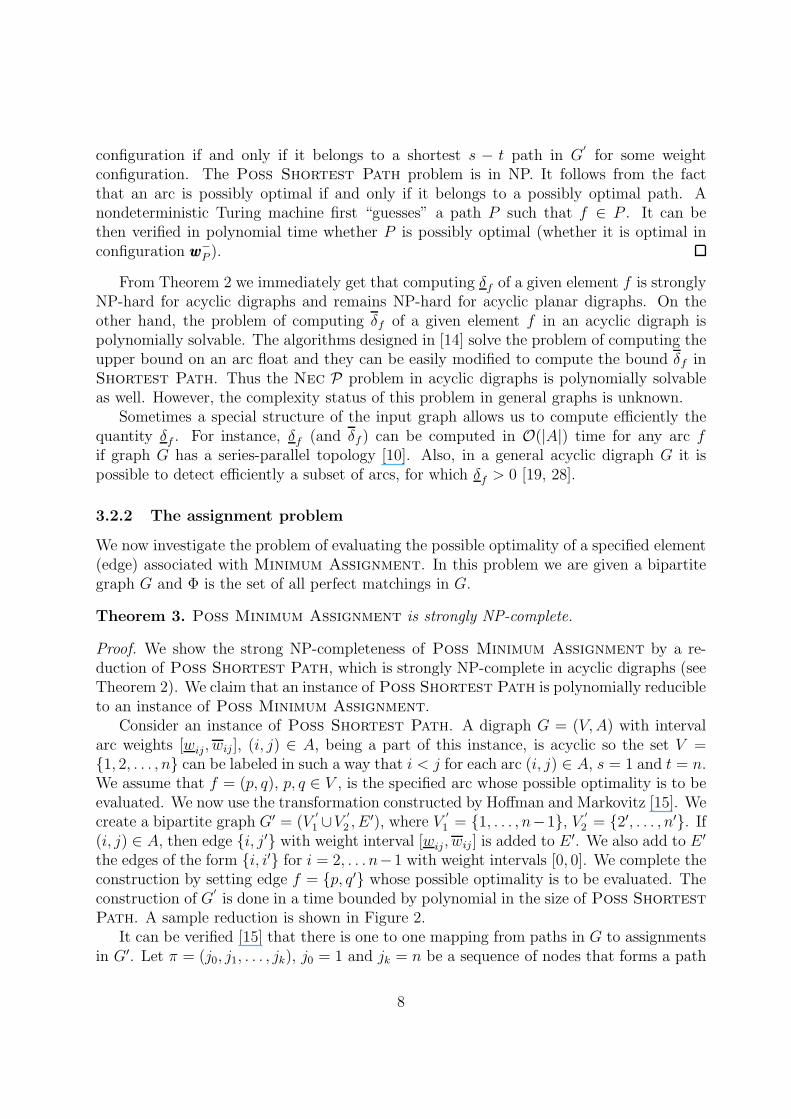
for some weightconfiguration. The Poss Shortest Path problem is in NP. It follows from the factthat an arc is possibly optimal if and only if it belongs to a possibly optimal path. Anondeterministic Turing machine first “guesses” a path P such that f ∈ P . It can bethen verified in polynomial time whether P is possibly optimal (whether it is optimal inconfiguration www−

P ).

From Theorem 2 we immediately get that computing δf of a given element f is stronglyNP-hard for acyclic digraphs and remains NP-hard for acyclic planar digraphs. On theother hand, the problem of computing δf of a given element f in an acyclic digraph ispolynomially solvable. The algorithms designed in [14] solve the problem of computing theupper bound on an arc float and they can be easily modified to compute the bound δf inShortest Path. Thus the Nec P problem in acyclic digraphs is polynomially solvableas well. However, the complexity status of this problem in general graphs is unknown.

Sometimes a special structure of the input graph allows us to compute efficiently thequantity δf . For instance, δf (and δf ) can be computed in O(|A|) time for any arc fif graph G has a series-parallel topology [10]. Also, in a general acyclic digraph G it ispossible to detect efficiently a subset of arcs, for which δf > 0 [19, 28].

3.2.2 The assignment problem

We now investigate the problem of evaluating the possible optimality of a specified element(edge) associated with Minimum Assignment. In this problem we are given a bipartitegraph G and Φ is the set of all perfect matchings in G.

Theorem 3. Poss Minimum Assignment is strongly NP-complete.

Proof. We show the strong NP-completeness of Poss Minimum Assignment by a re-duction of Poss Shortest Path, which is strongly NP-complete in acyclic digraphs (seeTheorem 2). We claim that an instance of Poss Shortest Path is polynomially reducibleto an instance of Poss Minimum Assignment.

Consider an instance of Poss Shortest Path. A digraph G = (V, A) with intervalarc weights [wij, wij ], (i, j) ∈ A, being a part of this instance, is acyclic so the set V =1, 2, . . . , n can be labeled in such a way that i < j for each arc (i, j) ∈ A, s = 1 and t = n.We assume that f = (p, q), p, q ∈ V , is the specified arc whose possible optimality is to beevaluated. We now use the transformation constructed by Hoffman and Markovitz [15]. Wecreate a bipartite graph G′ = (V

′

1 ∪V′

2 , E ′), where V′

1 = 1, . . . , n−1, V′

2 = 2′, . . . , n′. If(i, j) ∈ A, then edge i, j′ with weight interval [wij, wij ] is added to E ′. We also add to E ′

the edges of the form i, i′ for i = 2, . . . n−1 with weight intervals [0, 0]. We complete theconstruction by setting edge f = p, q′ whose possible optimality is to be evaluated. Theconstruction of G

′is done in a time bounded by polynomial in the size of Poss Shortest

Path. A sample reduction is shown in Figure 2.It can be verified [15] that there is one to one mapping from paths in G to assignments

in G′. Let π = (j0, j1, . . . , jk), j0 = 1 and jk = n be a sequence of nodes that forms a path

8

[1, 2]

[1, 2]

[1, 4]

[1, 4]

[0, 2]

[0, 2]

[3, 5]

[3, 5]

[0, 1][0, 1]

[0, 0]

[0, 0]2′

3′

4′

1

1

2

2

3

3

4

Figure 2: An instance of Poss Shortest Path and the corresponding instance of Poss

Minimum Assignment.

in G. The corresponding assignment A is constructed as follows: node ji is paired with j′i+1

for i = 0, . . . , k − 1; every node j /∈ π is paired with j′. On the other hand, let A ⊂ E bean assignment in G′. It must contain the subset of edges j0, j

′1, j1, j

′2, . . . , jk−1, j

′k,

where j0 < j1 < · · · < jk−1 < n, j0 = 1 and jk = n. Moreover, it is not difficult to verifythat if j /∈ j0, . . . , jk−1 and j 6= n, then edge j, j′ must belong to A. Observe that thesequence of nodes (j0, j1, . . . , jk) is a path from 1 to n in G.

From the construction of G′, it follows that one can use www to denote the same configu-ration of weights both in G and G′. It follows from the fact that all the additional edgesin G′ have degenerate weight intervals [0,0]. For any configuration www each path π from 1to n in G has a corresponding assignment A of the same weight in G′ and the converseis also true. Consequently, an optimal path π∗ in www gives an optimal assignment A∗ in wwwand vice versa. Moreover, (p, q) ∈ π∗ if and only if p, q′ ∈ A∗. Thus arc g = (p, q) ispossibly optimal in Shortest Path if and only if f = p, q′ is possibly optimal in thecorresponding Minimum Assignment. The Poss Minimum Assignment problem is inNP and the proof is similar to the proof in Theorem 2.

We can thus see that computing the value of δf in Minimum Assignment is strongly

NP-hard. However, the complexity status of the problems of computing δf and checkingthe necessary optimality of edge f is unknown.

3.2.3 The minimum s-t cut problem

Consider the problem of evaluating the optimality of a specified element (arc) f associatedwith Minimum s-t Cut. In this problem Φ consists of all s − t cuts in a given directedgraph G. If V1 ∪V2 is a partition of the node set V such that s ∈ V1 and t ∈ V2, then a cutis formed by all arcs that start in V1 and end in V2. We will show that Poss Minimum

s-t Cut is computationally intractable even if an input graph is planar. Recall that agraph is planar if it can be embedded in the plane without crossing arcs. An embedding ofa planar digraph partitions the plane into separate regions called faces. Exactly one suchface is unbounded and it is called the outer face. A right face of an arc a = (i, j) ∈ A is theface which is on the right hand side of (i, j) when traversing this arc from i to j. Similarlywe define the left face of a.

9

Suppose that G = (V, A) is a directed planar graph with two distinguished nodes sand t. We assume, without loss of generality, that no arc enters s and no arc leaves t.Such arcs can be removed from G because they cannot be a part of any cut in G. We alsoassume that G is given as a plane representation, in which s and t touch the outer face.The digraph G is associated with a digraph G∗ = (V ∗, A∗) called a dual digraph. The dualdigraph is constructed as follows. We first modify G by introducing an artificial arc (t, s)in the outer face of G, so that this arc is directed clockwise when looking from the insideof G. The nodes of G∗ are the faces of the modified digraph G. For every arc a ∈ A, exceptfor the artificial one, we add to A∗ arc a∗ that intersects a and joins the nodes in the faceson either side of it; arc a∗ = (i∗, j∗) is oriented in such a way that node i∗ is in the rightface of a = (i, j). Finally, s∗ ∈ V ∗ is the node corresponding to the face limited by theartificial arc (t, s) in G and t∗ ∈ V ∗ is the node that corresponds to the outer face of G. Itis easy to verify that G∗ is also a planar digraph and the dual of G∗ is G. An example ofa planar digraph and its dual are shown in Figure 3. The construction of the dual graphG∗ can be done in polynomial time (see, e.g.[1, 23]).

e1

e2

e3

e4

e5

s t

e∗1

e∗2

e∗3

e∗4

e∗5

s∗

t∗ G∗

G

Figure 3: Construction of a dual graph G∗ (dashed arcs).

Let V1 ∪ V2 be a partition of V such that s ∈ V1 and t ∈ V2. A cut C, that correspondsto this partition, is said to be uniformly directed s − t cut if no arcs in G lead from V2 toV1. The following theorem characterizes a planar digraph and its dual:

Theorem 4 ([1, 23]). Let G be a planar acyclic digraph and let G∗ be its dual. Then

P = a1, a2, . . . , ak is a simple path from s to t in G if and only if C = a∗1, a

∗2, . . . , a

∗k is

an uniformly directed s∗ − t∗ cut in G∗

Hence there is one-to-one correspondence between simple paths in a directed planargraph and uniformly directed cuts in its dual. We will use this fact to prove the followingresult:

Theorem 5. Poss Minimum s-t Cut is NP-complete for planar digraphs.

Proof. We will construct a polynomial time reduction from Poss Shortest Path foracyclic planar digraphs, which is known to be NP-complete (see Theorem 2). Let an

10

acyclic planar digraph G = (V, A), s ∈ V , t ∈ V , with interval arc weights [wa, wa], a ∈ A,and a specified arc f = (k, l) ∈ A be an instance of Poss Shortest Path. We constructthe corresponding instance of Poss Minimum s-t Cut as follows. We first construct adual digraph G∗ = (V ∗, A∗) for G. The interval weight of arc a∗ ∈ A∗ is the same as theinterval weight of the corresponding arc a ∈ A. Then for every arc a∗ = (i∗, j∗) ∈ A∗ wecreate the reverse arc b∗ = (j∗, i∗) with interval weight [M, M ]. This arc is called a dummy

arc. We fix M = |A|wmax + 1, where wmax = maxa∈A wa. We denote by G∗∗ the resultingdigraph with dummy arcs. Finally, we distinguish arc f ∗ in G∗∗. It is easily seen thatdigraph G∗∗ is planar and it can be constructed from G in polynomial time. A samplereduction is shown in Figure 4.

a1

f

a3a4

a5

a6

a7

s t

a∗1

b∗1

f∗ b∗2

a∗3

b∗3a∗5

b∗5

a∗6

b∗6

a∗7

b∗7

b∗4

a∗4

s∗

t∗

Figure 4: A sample reduction. Arcs a∗i have the same interval weights as ai and arcs b∗i

have interval weights [M, M ].

We claim that arc f ∗ belongs to a minimum cut in G∗∗ under some weight configurationif and only if f belongs to a shortest path in G under some weight configuration.

Observe first that every uniformly directed cut C in G∗ is a cut in G∗∗. It followsfrom the fact that adding dummy arcs to G∗ only backward arcs leading from V2 to V1

are created, where V1 ∪ V2 is a partition of nodes that corresponds to cut C. Considera configuration www in G∗∗. A minimum cut under www cannot use any dummy arc. Indeed,there is at least one cut in G∗∗ that does not use any dummy arc. To see this considera path from s to t in G. This path corresponds to a uniformly directed cut C in G∗ andobviously C is also the cut in G∗∗. Every cut C1 in G∗∗, that uses a dummy arc, has theweight of at least |A|wmax + 1, which is strictly greater than the weight of C under www.Consequently, C1 cannot be a minimum cut under www. Now from Theorem 4 we get thatpath P = a1, a2, . . . , ak is a shortest path in G under some weight configuration if andonly if cut C = a∗

1, a∗2, . . . , a

∗k is a minimum cut in G∗∗ under some weight configuration.

Moreover, f ∈ P if and only if f ∗ ∈ C. Poss Minimum s-t Cut is in NP and thereasoning is the same as for Poss Shortest Path in Theorem 2.

Similarly to Poss Minimum Assignment and Poss Shortest Path, computingδf for a given arc f in the considered problem is NP-hard. However, the problems of

11

computing δf and asserting whether f is necessarily optimal remain open.

4 Fuzzy combinatorial optimization problem

In this section, we discuss a fuzzy version of problem P, that is problem P with uncertainweights modeled by fuzzy intervals. We provide a possibilistic interpretation of the fuzzyproblem together with some solution concepts, which can be viewed as a generalization ofthe minmax regret approach.

4.1 Some basic notions of possibility theory

A fuzzy set (see [11]) A is a reference set Ω together with mapping µ eAfrom Ω into [0, 1],

called a membership function. The value of µ eA(v), v ∈ Ω, is interpreted as the degree

of membership of v in the fuzzy set A. A λ-cut, λ ∈ (0, 1], of A is a classical set, i.e.

Aλ = v ∈ Ω : µ eA(v) ≥ λ. The cuts of A form a family of nested sets, i.e if λ1 ≥ λ2, then

Aλ1 ⊆ Aλ2 . A fuzzy set in R, whose membership function is normal, quasi-concave andupper semi-continuous is called a fuzzy interval (see [11]). A support of a fuzzy interval A

is the set v : µ eA(v) > 0 together with its closure and it will be denoted as A0. We will

assume that the support of a fuzzy interval is bounded. It can be shown [11] that if A is

a fuzzy interval with a bounded support, then Aλ is a closed interval for every λ ∈ [0, 1].

We can thus represent a fuzzy interval A as a family of cuts Aλ = [aλ, aλ], λ ∈ [0, 1]. Onecan obtain the membership function µ eA from the family of λ-cuts in the following way:

µ eA(v) = supλ ∈ [0, 1] : v ∈ Aλ (3)

and µ eA(v) = 0 if v /∈ A0. Observe that a classical closed interval A = [a, a] is a special caseof a fuzzy one with membership function µA(v) = 1 if v ∈ A and µA(v) = 0 otherwise. Inthis case we have Aλ = [a, a] for all λ ∈ [0, 1]. Another class of fuzzy intervals is formedby trapezoidal fuzzy intervals, denoted as (a, a, αA, βA), αA, βA > 0. In this case we haveAλ = [a − (1 − λ)αA, a + (1 − λ)βA] for λ ∈ [0, 1].

Let us now recall a possibilistic interpretation of a fuzzy set. Possibility theory [11]is an approach to handle incomplete information with two dual measures: possibility andnecessity, which are used to model available information. Both measures are built froma possibility distribution. Let a fuzzy set A be attached with a single-valued variable a.The membership function µ eA is a possibility distribution, πa = µ eA, which describes theset of more or less plausible, mutually exclusive values of the variable a. It is similar to aprobability density. The value of πa(v) represents the possibility degree of the assignmenta = v, i.e. Π(a = v) = πa(v) = µ eA

(v). In particular, πa(v) = 0 means that a = vis impossible and πa(v) > 0 means that a = v is plausible. A degree of possibility canbe viewed as an upper bound of a degree of probability. A detailed interpretation of thepossibility distribution and some methods of obtaining it from the possessed knowledge are

12

described in [11]. The possibility of an event “a ∈ B”, denoted by Π(a ∈ B), is as follows:

Π(a ∈ B) = supv

minπa(v), µB(v), (4)

where B can be a fuzzy set. Π(a ∈ B) evaluates the extent to which “a ∈ B” is possiblytrue. If B is a subset of R, then µB is a characteristic function of B and thus Π(a ∈ B) =supv∈B πa(v). The necessity of an event “a ∈ B”, denoted by N(a ∈ B), is as follows:

N(a ∈ B) = 1−Π(a ∈ B) = 1−supv

minπa(v), 1−µB(v) = infv

max1−πa(v), µB(v), (5)

where B is the complement of B and its membership function is µB = 1 − µB. N(a ∈ B)evaluates the extent to which “a ∈ B” is certainly true. If B is a subset of R, thenN(a ∈ B) = infv 6∈B(1 − πa(v)).

4.2 Fuzzy combinatorial optimization problem in the setting of

possibility theory

We now present a possibilistic formalization of problem P, in which uncertainty of theelement weights is modeled by fuzzy intervals We, e ∈ E. A membership function ofWe is regarded as a possibility distribution for the values of the unknown weight we, i.e.πwe

= µfWe, e ∈ E. Thus the possibility degree of the assignment we = v is Π(we =

v) = πwe(v) = µfWe

(v). Let www = (ve)e∈E be a configuration of the element weights. Theconfiguration www represents a state of the world in which we = ve, for all e ∈ E. It definesan instance of problem P with the deterministic weights (ve)e∈E. Assuming that weightsare unrelated to one another, the degree of possibility of a configuration www = (ve)e∈E is

obtained by the following joint possibility distribution on configurations induced by We,e ∈ E (see [10, 12]):

π(www) = Π(∧e∈E(we = ve)) = mine∈E

Π(we = ve) = mine∈E

µfWe(ve).

Let us denote by Pλ, λ ∈ [0, 1], the interval-valued problem P with element weights W λe =

[wλe , w

λe ], e ∈ E. Note that the configuration set in Pλ is composed of all configurations

www such that π(www) ≥ λ, that is whose possibility of occurrence is not less than λ. In thenext sections we will show that the optimality evaluation and the problem of choosing asolution under fuzzy weights can be reduced to examining a family of interval problemsPλ, λ ∈ [0, 1]. In consequence, the results obtained for the interval-valued case can beapplied to the fuzzy problems as well.

4.2.1 The optimality evaluation and fuzzy deviation interval

According to possibility theory, the degrees of possibility and necessity that a solutionX ∈ Φ is optimal are defined as follows:

Π(X is optimal) = supwww:X is optimal to P for www

π(www), (6)

N(X is optimal) = 1 − Π(X is not optimal) = infwww:X is not optimal to P for www

(1 − π(www)).(7)

13

Similarly, the degrees of possibility and necessity that an element f ∈ E is optimal aredefined as follows:

Π(f is optimal) = supwww:f is optimal to P for www

π(www), (8)

N(f is optimal) = 1 − Π(f is not optimal) = infwww:f is not optimal to P for www

(1 − π(www)). (9)

It is easy to check that Π(X is optimal) ≤ mine∈X Π(e is optimal) and N(X is optimal) ≤mine∈X N(e is optimal).

We now show that, similarly to the interval-valued case (see Section 3), we can expressthe degrees of possible and necessary optimality in terms of a deviation interval. In thefuzzy case, however, the deviation interval becomes a fuzzy one and it represents a pos-sibility distribution for a solution (element) deviation. The possibility distribution thatrepresents more or less plausible values of deviation δX of a solution X is defined in thefollowing way:

Π(δX = v) = µ∆X(v) = sup

www: δX(www)=v

π(www), (10)

where Π(δX = v) stands for the possibility degree that δX = v. Since the statement“X is optimal under www” is equivalent to the condition δX(www) = 0, we get the followingrelationships between optimality degrees (6), (7) and deviation (10):

Π(X is optimal) = supwww:δX(www)=0

π(www) = Π(δX = 0) = µ∆X(0),

N(X is optimal) = 1 − supwww:δX(www)>0

π(www) = N(δX = 0) = 1 − supv>0

µ∆X(v).

Using (3) we can express µ∆Xin the following way:

µ∆X(v) = supλ : v ∈ ∆λ

X, (11)

where ∆λX = [δλ

X , δλ

X ], λ ∈ [0, 1], is the interval of possible values of deviation of solution

X in problem Pλ. It is easy to verify that δλX is a nondecreasing and δ

λ

X is a nonincreasingfunction of λ. We thus have

Π(X is optimal) = µ∆X(0) = supλ : 0 ∈ ∆λ

X = supλ : δλX = 0 (12)

and Π(X is optimal) = 0 if δ0X > 0. A similar reasoning leads to the following equality:

N(X is optimal) = 1 − infλ : δλ

X = 0 (13)

and N(X is optimal) = 0 if δ1

X > 0. Exactly the same reasoning can be applied to elements.It is enough to replace X with f in formulae (10)-(13).

Formulae (12) and (13) suggest a method for computing the optimality degrees. Inorder to compute the degree of possible optimality we need to find the largest value of

14

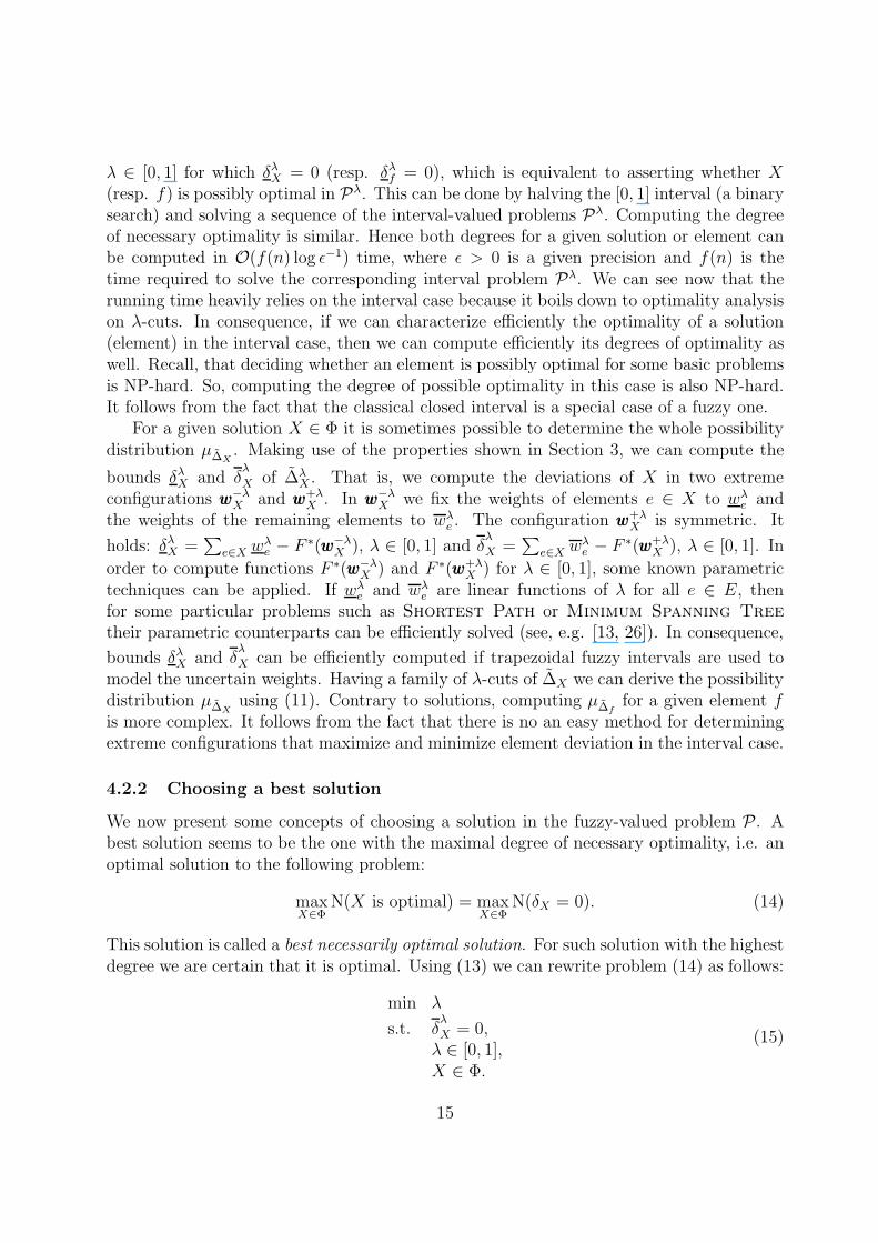
λ ∈ [0, 1] for which δλX = 0 (resp. δλ

f = 0), which is equivalent to asserting whether X(resp. f) is possibly optimal in Pλ. This can be done by halving the [0, 1] interval (a binarysearch) and solving a sequence of the interval-valued problems Pλ. Computing the degreeof necessary optimality is similar. Hence both degrees for a given solution or element canbe computed in O(f(n) log ǫ−1) time, where ǫ > 0 is a given precision and f(n) is thetime required to solve the corresponding interval problem Pλ. We can see now that therunning time heavily relies on the interval case because it boils down to optimality analysison λ-cuts. In consequence, if we can characterize efficiently the optimality of a solution(element) in the interval case, then we can compute efficiently its degrees of optimality aswell. Recall, that deciding whether an element is possibly optimal for some basic problemsis NP-hard. So, computing the degree of possible optimality in this case is also NP-hard.It follows from the fact that the classical closed interval is a special case of a fuzzy one.

For a given solution X ∈ Φ it is sometimes possible to determine the whole possibilitydistribution µ∆X

. Making use of the properties shown in Section 3, we can compute the

bounds δλX and δ

λ

X of ∆λX . That is, we compute the deviations of X in two extreme

configurations www−λX and www+λ

X . In www−λX we fix the weights of elements e ∈ X to wλ

e andthe weights of the remaining elements to wλ

e . The configuration www+λX is symmetric. It

holds: δλX =

∑e∈X wλ

e − F ∗(www−λX ), λ ∈ [0, 1] and δ

λ

X =∑

e∈X wλe − F ∗(www+λ

X ), λ ∈ [0, 1]. In

order to compute functions F ∗(www−λX ) and F ∗(www+λ

X ) for λ ∈ [0, 1], some known parametrictechniques can be applied. If wλ

e and wλe are linear functions of λ for all e ∈ E, then

for some particular problems such as Shortest Path or Minimum Spanning Tree

their parametric counterparts can be efficiently solved (see, e.g. [13, 26]). In consequence,

bounds δλX and δ

λ

X can be efficiently computed if trapezoidal fuzzy intervals are used tomodel the uncertain weights. Having a family of λ-cuts of ∆X we can derive the possibilitydistribution µ∆X

using (11). Contrary to solutions, computing µ∆ffor a given element f

is more complex. It follows from the fact that there is no an easy method for determiningextreme configurations that maximize and minimize element deviation in the interval case.

4.2.2 Choosing a best solution

We now present some concepts of choosing a solution in the fuzzy-valued problem P. Abest solution seems to be the one with the maximal degree of necessary optimality, i.e. anoptimal solution to the following problem:

maxX∈Φ

N(X is optimal) = maxX∈Φ

N(δX = 0). (14)

This solution is called a best necessarily optimal solution. For such solution with the highestdegree we are certain that it is optimal. Using (13) we can rewrite problem (14) as follows:

min λ

s.t. δλ

X = 0,λ ∈ [0, 1],X ∈ Φ.

(15)

15

If problem (15) is infeasible then N(X is optimal) = 0 for all X ∈ Φ. The constraint

δλ

X = 0 stands for the necessary optimality of X in the interval-valued problem Pλ. Theproblem (15) can be solved in polynomial time if problem P with deterministic weights ispolynomially solvable. An algorithm is based on a binary search, that is, we halve the unitinterval of possible values of λ to compute the minimum value of λ such that there exists anecessarily optimal solution in the interval-valued problem Pλ. At each iteration finding anecessarily optimal solution, if it exists, can be done in polynomial, say in f(n), time (seeSection 3). Thus the overall complexity of the algorithm is O(f(n) log ǫ−1), where ǫ > 0 isa given precision.

The criterion of choosing a solution used in (14) is very strong. Namely, a solution Xsuch that N(X is optimal) > 0 may not exist or even if it exists, its necessary optimalitydegree may be very small. We apply now a more soft solution concept originally proposedfor fuzzy linear programming in [17, 18]. The idea consists in replacing the optimalityrequirement for a solution (δX = 0) with a suboptimality one. Let us introduce a fuzzy

goal G on the value of the deviation of X, where µ eG : [0, +∞) → [0, 1] is a nonincreasingfunction such that µ eG

(0) = 1. Function µ eGis given in advance and the value of µ eG

(δX)expresses the degree to which deviation δX satisfies a decision maker. The degree ofnecessity that a solution X is soft optimal is defined as follows [17, 18]:

N(X is soft optimal) = infwww

max1 − π(www), µ eG(δX(www)). (16)

Using (5) we can check that N(X is soft optimal) = N(δX ∈ G). N(X is soft optimal) = αmeans that for all configurations www such that π(www) > 1 − α it holds µ eG

(δX(www)) ≥ α or

equivalently δX(www) ∈ Gα = [0, µ−1eG

(α)], which represents the suboptimality of X. Function

µ−1eG

: [0, 1] → R ∪ +∞ is a pseudo-inverse of µ eG that is µ−1eG

(α) = supv : µ eG(v) ≥ α.

Observe that if we define µ eG(0) = 1 and µ eG

(x) = 0 for x > 0, then N(X is soft optimal) =N(X is optimal). Now, a more reasonable solution is an optimal one to the followingproblem:

maxX∈Φ

N(X is soft optimal). (17)

This solution is called a best necessarily soft optimal solution. It can be shown (the proofis similar to that in [18]) that problem (17) is equivalent to the following one:

min λ

s.t. δλ

X ≤ µ−1eG

(1 − λ),

λ ∈ [0, 1],X ∈ Φ.

(18)

If problem (18) is infeasible then N(X is soft optimal) = 0 for all solutions X ∈ Φ. If λ∗ isthe optimal objective value of (18) and X is the best necessarily soft optimal solution, then

N(X is soft optimal) = 1 − λ∗. Since δλ

X is nonincreasing and µ−1eG

(1 − λ) is nondecreasing

function of λ, problem (18) can also be solved by a binary search on λ ∈ [0, 1]. We must

16

find the smallest value of λ for which condition δλ

X ≤ µ−1eG

(1 − λ) is satisfied for some

solution X ∈ Φ. Since δλ

X is the maximal regret of X in Pλ, a solution that minimizes δλ

X

is an optimal minmax regret solution in Pλ. We thus can see that problem (18) consistsof solving a family of minmax regret Pλ problems. Hence the concept of a necessarysoft optimality is a natural extension of the minmax regret approach to the fuzzy case.Therefore, solving (18) is more complex than solving (15) and it depends on the complexityof the minmax regret version of problem P.

5 Conclusions

In this paper, we have studied a general combinatorial optimization problem with ill-knownelement weights modeled by closed intervals and fuzzy intervals. Our aim was to presentsome general concepts and some relationships among them. We have discussed first theinterval-valued case and then we have shown how the notions introduced for the interval-valued problem can be naturally generalized to the fuzzy-valued one. We have also exploredsome computational aspects of the optimality evaluation. We have seen that characterizingthe optimality of elements is, in general, more complex than characterizing the optimalityof solutions.

The fuzzy problem has an interpretation in the setting of possibility theory. Applyingthis theory we can describe the notion of optimality and choose a robust solution underimprecision. The possibilistic analysis appears to be much easier than a probabilisticmodeling. In particular, the computation of the possibility distribution of a solution orelement deviation in a possibilistic framework is easier, than with a probabilistic model.

We have shown that the optimality evaluation and choosing a solution in the fuzzyproblem is not harder than in the interval-valued case. In fact, every fuzzy problem boilsdown to solving a small number of interval problems. Thus the interval uncertainty repre-sentation seems to be a core problem in which the combinatorial structure of problem Pplays a crucial role. Every result obtained for the interval problem can also be applied toits fuzzy counterpart as well. Furthermore, if some problem is hard in the interval case,then its fuzzy counterpart is not easier.

Acknowledgements

This work was partially supported by Polish Committee for Scientific Research, grant NN111 1464 33.

References

[1] V. Adlakha, B. Gladysz, J. Kamburowski, Minimum Flows in (s,t) Planar Networks,Networks 21 (1991) 767–773.

17

[2] H. Aissi, C. Bazgan, D. Vanderpooten, Complexity of the min-max (regret) versions ofcut problems, ISAAC 2005, LNCS 3827, pp. 789–798, 2005.

[3] H. Aissi, C. Bazgan, D. Vanderpooten, Complexity of the min-max and min-max regretassignment problems, Operations Research Letters 33 (2005) 634–640.

[4] H. Aissi, C. Bazgan, D. Vanderpooten, Min-max and min-max regret versions of com-binatorial optimization problems: A survey, European Journal of Operational Research

to appear 2009, doi:10.1016/j.ejor.2008.09.012.

[5] I. D. Aron, P. van Hentenryck, On the complexity of the robust spanning tree problemwith interval data, Operations Research Letters 32 (2004) 36–40.

[6] I. Averbakh, V. Lebedev, Interval data minmax regret network optimization problems,Discrete Applied Mathematics 138 (2004) 289–301.

[7] I. Averbakh, V. Lebedev, On the complexity of minmax regret linear programming,European Journal of Operational Research 160 (2005) 227–231.

[8] S. Chanas, P. Zielinski, The computational complexity of the criticality problems ina network with interval activity times, European Journal of Operational Research 136(2002) 541–550.

[9] S. Chanas, P. Zielinski, On the hardness of evaluating criticality of activities in a planarnetwork with duration intervals, Operations Research Letters 31 (2003) 53–59.

[10] D. Dubois, H. Fargier, V. Galvagnon, On latest starting times and floats in activ-ity networks with ill-known durations, European Journal of Operational Research 147(2003) 266–280.

[11] D. Dubois, H. Prade, Possibility theory: an approach to computerized processing of

uncertainty, Plenum Press, New York 1988.

[12] D. Dubois, H. Fargier, P. Fortemps, Fuzzy scheduling: modelling flexible constraintsvs. coping with incomplete knowledge, European Journal of Operational Research 147(2003) 231–252.

[13] D. Fernandez-Baca, G. Slutzki, D. Eppstein, Using sparsification for parametric min-imum spanning tree problems, SWAT 1996, LNCS 1097, pp. 149–160, 1996.

[14] J. Fortin, P. Zielinski, D. Dubois, H. Fargier, Interval analysis in scheduling, CP 2005,LNCS 3709, pp. 226–240, 2005.

[15] A.J. Hoffman, H. Markowitz, A note on shortest path, assignment and transportationproblems, Naval Research Logistics Quarterly 10 (1963) 375–379.

[16] M. Inuiguchi, Minimax regret solution to linear programming problems with an inter-val objective function, European Journal of Operational Research 86 (1995) 526–536.

18

[17] M. Inuiguchi, On Possibilistic / Fuzzy Optimization, IFSA 2007, LNAI 4527, pp.351–360, 2007.

[18] M. Inuiguchi, M. Sakawa, Robust optimization under softness in a fuzzy linear pro-gramming problem, International Journal of Approximate Reasoning 18 (1998) 21–34.

[19] O. E. Karasan, M. C. Pinar, H. Yaman, The robust shortest path problem with intervaldata. Industrial Engineering Department, Bilkent University, 2001.

[20] A. Kasperski, P. Zielinski, An approximation algorithm for interval data minmaxregret combinatorial optimization problems, Information Processing Letters 97 (2006)177–180.

[21] A. Kasperski, P. Zielinski, On combinatorial optimization problems on matroids withuncertain weights, European Journal of Operational Research 177 (2007) 851-864.

[22] P. Kouvelis, G. Yu, Robust Discrete Optimization and its applications. Kluwer Aca-demic Publishers, Boston 1997.

[23] E. L. Lawler, Combinatorial Optimization: Networks and Matroids. Holt, Rinehartand Winston, New York 1976.

[24] R. Montemanni, L. M. Gambardella, A. V. Donati, A branch and bound algorithmfor the robust shortest path problem with interval data, Operations Research Letters

32 (2004) 225–232.

[25] S. Okada, Fuzzy shortest path problems incorporating interactivity among paths,Fuzzy Sets and Systems 142 (2004) 335–357.

[26] N. Young, R. Tarjan, J. Orlin, Faster Parametric Shortest Path and Minimum BalanceAlgorithms, Networks 21 (1991) 205–221.

[27] H. Yaman, O. E. Karasan, M. C. Pinar, The robust spanning tree problem withinterval data, Operations Research Letters 29 (2001) 31–40.

[28] P. Zielinski, On computing the latest starting times and floats of activities in a networkwith imprecise durations, Fuzzy Sets and Systems 150 (2005) 53-76.

19