1

Sub-optimality of Treating Interference as

Noise in the Cellular Uplink with Weak

InterferenceSoheil Gherekhloo, Chen Di, Anas Chaaban, and Aydin Sezgin

Institute of Digital Communication Systems

Ruhr-Universitat Bochum

Email: soheyl.gherekhloo,di.chen,anas.chaaban,aydin.sezgin@rub.de

Abstract

Despite the simplicity of the scheme of treating interference as noise (TIN), it was shown to be sum-capacity

optimal in the Gaussian interference channel (IC) with very-weak (noisy) interference. In this paper, the 2-user IC is

altered by introducing a further transmitter that wants to communicate with one of the receivers of the IC. The resulting

network thus consists of a point-to-point channel interfering with a multiple access channel (MAC) and is denoted

PIMAC. The sum-capacity of the PIMAC is studied with main focus on the optimality of TIN. It turns out that TIN in

its naïve variant, where all transmitters are active and both receivers use TIN for decoding, is not the best choice for

the PIMAC. In fact, a scheme that combines both time division multiple access and TIN (TDMA-TIN) outperforms

the naïve TIN scheme. Furthermore, it is shown that in some regimes, TDMA-TIN achieves the sum-capacity for

the deterministic PIMAC and the sum-capacity within a constant gap for the Gaussian PIMAC. Additionally, it is

observed that, even for very-weak interference, there are some regimes where a combination of interference alignment

and TIN outperforms TDMA-TIN.

I. INTRODUCTION

Communicating nodes in most communication systems existing nowadays have several practical constraints. One

such constraint is the limited computational capability of the receiving nodes. This limitation demands communication

schemes which do not have a high decoding complexity. However, communication over networks where concurrent

transmissions takes place (interference networks) challenges the receivers with additional complexity, namely,

the complexity of interference management. Most near-optimal schemes in interference networks require some

computation at the receiver side, and thus, increase the computational complexity.

One common way to avoid this problem is the simple scheme of treating interference as noise (TIN). In this

scheme, the receivers’ strategy is the same as if there were no interference at all, i.e., interference is ignored. TIN

This paper is a revised and extended version of the conference paper [1].

February 3, 2014 DRAFT

arX

iv:1

401.

8265

v1 [

cs.I

T]

31

Jan

2014

2

over the interference channel (IC) has been studied by several researchers (see [2], [3] and references therein).

Although seemingly a very trivial scheme, TIN is optimal in the IC with very-weak interference. The very-weak

interference condition was identified in [4] as INR <√

SNR where it was shown that TIN achieves the sum-capacity

of the 2-user IC within a gap of 1 bit. This fact was refined in [5]–[7] where it was shown that TIN achieves the

exact sum-capacity of the 2-user IC with noisy interference, a smaller regime than the very-weak interference regime

introduced in [4]. In a similar spirit, the very-weak interference regime for the K-user (K > 2) IC was identified in

[8]. In [9] it was shown that TIN achieves the capacity region of the fully asymmetric K-user IC within a constant

gap as long as the sum of the powers of the strongest interference caused by a user plus the strongest interference

it receives is less than the power of its desired signal, on a logarithmic scale. Furthermore, the sum-capacity of the

K-user IC with noisy interference was characterized in [10].

In this paper, we study the impact of introducing one more transmitter (without introducing a new receiver) to the

2-user IC on TIN. We consider a network consisting of a point-to-point (P2P) channel interfering with a multiple

access channel (MAC). We call this network a PIMAC. Such a setup might arise if a P2P communication system

uses the same communication medium as a cellular uplink for instance. The PIMAC setup was studied in [11] where

its capacity region in strong and very strong interference cases was obtained and a sum-capacity upper bound was

derived, and in [12] where an achievable rate region for the discrete memoryless Z-PIMAC (partially connected

PIMAC) was provided, which achieves the capacity of the Z-PIMAC with strong interference.

The PIMAC was also considered in [13] where the sum-capacity of the deterministic PIMAC (under some

conditions on the channel parameters) was given. In more details, the work of Bühler and Wunder in [13] established

the sum-capacity of the deterministic PIMAC under the following symmetry consideration: The power of the

interference caused by the MAC transmitters at the P2P receiver is equal. For this case, the authors of [13] have

derived the sum-capacity of the deterministic PIMAC and have shown that it is larger than that of the deterministic

IC.

In this paper, we consider both the deterministic model and the Gaussian model of the PIMAC without the above

constraint of equal power of interference from the MAC transmitters to the P2P receiver. The main focus of the paper

is to study the performance of the simple scheme of TIN in the PIMAC in terms of achievable rates. The question

we would like to answer here is: Does TIN achieve the sum-capacity of the PIMAC in the noisy interference regime

as in the K-user IC? The difference between the PIMAC and the IC is in the existence of one more transmitter.

Moreover, TIN is optimal in the IC with noisy interference. Now by introducing one further transmitter to an IC

with noisy interference, one receiver (the P2P receiver of the PIMAC) experiences one more interferer. We focus

on the impact of this interferer under the condition above, i.e., the IC formed by removing one MAC transmitter

has noisy interference. Therefore, we put no restriction on the interference caused by the additional transmitter. The

performance of TIN is examined in the resulting PIMAC.

We distinguish between two variants of TIN: Naïve TIN and TDMA-TIN. Naïve TIN corresponds to the case

where each system (the MAC and the P2P) uses its interference free capacity achieving scheme. Notice that the

capacity achieving scheme in the interference free MAC is known (successive decoding), and so is that in the

February 3, 2014 DRAFT

3

interference free P2P channel [14]. In the presence of interference, the receivers proceed with decoding using their

interference-free optimal decoders while treating interference as noise. TDMA-TIN on the other hand corresponds

to the case where the MAC transmitters share the time resources, and the receivers treat interference as noise. Note

that in this case, the PIMAC is reduced into two 2-user IC’s operating over orthogonal resources (time slots).

We compare the two variants of TIN in the linear-deterministic [15] PIMAC first. By deriving new sum-capacity

upper bounds, we show that TDMA-TIN is sum-capacity achieving for a wide range of parameters, while naïve TIN

is optimal for a smaller range of channel parameters. Interestingly, we show that there exists a regime where one

MAC interference is noisy and the other interference is strong, where TIN is the optimal scheme. Intuitively, this

corresponds to the case where one MAC transmitter has a strong channel to the undesired receiver, and a weaker

channel to the desired receiver. In this case, it is better to silence this transmitter for the sake of achieving higher

sum-rates. The TDMA-TIN scheme achieves the sum-capacity in this case. It turns out also that there exists a sub-

regime where TDMA-TIN is not optimal and is outperformed by a scheme which exploits interference alignment.

Interestingly, this sub-regime includes cases where all interference links are very-weak but still TIN is not optimal.

Then, we consider the Gaussian PIMAC where we introduce new sum-capacity upper bounds. We identify regimes

where naïve TIN achieves the sum-capacity of the channel within a constant gap. Additionally, we show that although

naïve TIN achieves the sum-capacity of the channel within a constant gap for a range of channel parameters, it is

strictly outperformed by TDMA-TIN, and hence, is never sum-capacity optimal. This is in contrast to the K-user

IC where naïve TIN is optimal in the noisy interference regime. This clearly indicates that TDMA-TIN achieves

the sum-capacity within a constant gap in the same regimes where naïve TIN does. We also show that TDMA-

TIN achieves the sum-capacity of the channel within a constant gap in further regimes where naïve TIN does not.

Interestingly, while in the interference free MAC, successive decoding performs the same as TDMA in terms of

sum-capacity, the same is not true in the presence of interference with TIN. Next, we show there exist regimes of

the PIMAC with very-weak interference, where TDMA-TIN can not achieve the sum-capacity of the PIMAC within

a constant gap. We do this by extending the aforementioned schemes for the deterministic PIMAC to the Gaussian

PIMAC, deriving their achievable rates, and showing that the achievable rates are higher than those of TDMA-TIN

at high SNR.

The rest of the paper is organized as follows. In Section II, the PIMAC is introduced. Then the deterministic

PIMAC is studied in Section III where the sum-capacity is characterized under some conditions. Next, the Gaussian

PIMAC is discussed in Section IV with a comparison between different schemes and upper bounds. Finally, we

conclude with Section V.

Notation: Throughout the paper, we use F2 to denote the binary field and ⊕ to denote the modulo 2 addition. We

use normal lower-case, normal upper-case, boldface lower-case, and boldface upper-case letters to denote scalars,

scalar random variables, vectors, and matrices, respectively. x[a:b] denotes the vector formed by the a-th to b-th

components of vector x. We write X ∼ CN (0, P ) to indicate that the random variable X is distributed according

to a circularly symmetric complex normal distribution with zero mean and variance P . Furthermore, we define x+

as max{0, x}, and xn as the length-n sequence (x[1], · · · , x[n]). The vector 0q denotes the zero-vector of length

February 3, 2014 DRAFT

4

q, the matrix Iq is the q × q identity matrix, and xT denotes the transposition of a x.

II. SYSTEM MODEL

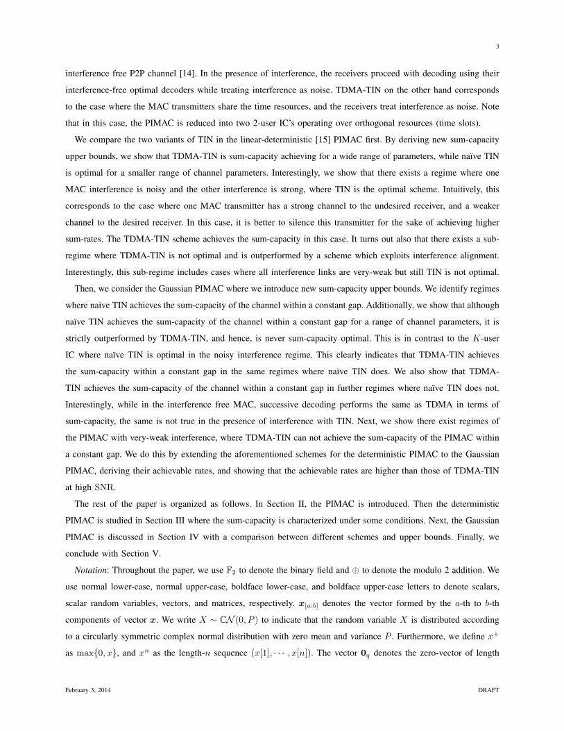
The system we consider consists of a P2P channel interfering with a MAC (PIMAC). As shown in Fig. 1, each

transmitter has a message to be sent to one receiver. Namely, transmitters 1 (TX1) and transmitter 3 (TX3) want

to send the messages W1 and W3, respectively, to receiver 1 (RX1), and transmitter 2 (TX2) wants to send the

message W2 to receiver 2 (RX2). The message Wi is a random variable, uniformly distributed over the message set

Wi = {1, · · · , b2nRic} where Ri denotes the rate of the message.

Fig. 1: The message flow in the PIMAC where the solid arrows indicate desired message flow and dashed arrows indicate interference.

To send its message, each transmitter uses an encoding function fi to map the message Wi into a codeword of

length n symbols Xni ∈ Cn. After the transmission of all n symbols of the codewords, RX1 has Y n1 and decodes

W1 and W3 by using a decoding function g1. RX1 thus obtains (W1, W3) = g1(Y n1 ). Similarly RX2 receives Y n2

and decodes W2 by using a decoding function g2, i.e., W2 = g2(Y n2 ). The messages sets, encoding functions, and

decoding functions constitute a code for the channel which is denoted an (n, 2nR1 , 2nR2 , 2nR3) code.

An error Ei occurs if Wi 6= Wi for some i ∈ {1, 2, 3}. A code for the PIMAC induces an average error probability

P(n) defined as

P(n) =1

2nRΣ

∑W∈W1×W2×W3

Prob

(3⋃i=1

Ei

), (1)

where RΣ =∑3i=1Ri and W = (W1,W2,W3). Reliable communication takes place if this error probability can

be made small by increasing n. This can occur if the rate triple (R1, R2, R3) satisfies some achievability constraints

which need to be found. The achievability of a rate triple (R1, R2, R3) is defined as the existence of a reliable

coding scheme which achieves these rates. In other words, a rate triple (R1, R2, R3) is said to be achievable if

there exists a sequence of (n, 2nR1 , 2nR2 , 2nR3) codes such that P(n) → 0 as n→∞. The set of all achievable rate

triples is the capacity region of the PIMAC denoted by C. In this paper, we focus is on the sum-capacity defined

as the maximum achievable sum-rate, i.e.,

CΣ = max(R1,R2,R3)∈C

RΣ. (2)

We consider a Gaussian PIMAC in this paper and study its sum-capacity. Next we introduce the specifics of the

Gaussian case.

February 3, 2014 DRAFT

5

A. Gaussian Model

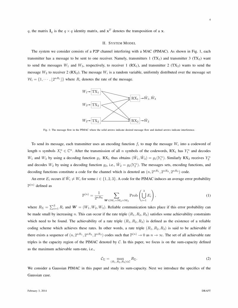
In the Gaussian PIMAC, the received signals of the two receivers at time index t ∈ {1, · · · , n} (denoted y1[t]

and y2[t]) can be written as1

y1[t] = hdx1[t] + hcx2[t] + hβx3[t] + z1[t], (3)

y2[t] = hcx1[t] + hdx2[t] + hαx3[t] + z2[t], (4)

where xi[t], i ∈ {1, 2, 3}, is a realization of the random variable Xi which represents the transmit symbol of

TXi, and zj [t], j ∈ {1, 2}, is a realization of random variable Zj ∼ CN (0, 1) which represents the additive white

Gaussian noise (AWGN), and the constants hd, hc, hβ , and hα represent the complex (static) channel coefficients.

We assume that global CSI is available to all nodes. Note that the noises Z1 and Z2 are independent from each

other and are both independent and identically distributed (i.i.d.) over time. The transmitters of the Gaussian PIMAC

have power constraints P which must be satisfied by their transmitted signals. Namely, the condition

1

n

n∑t=1

E[Xi[t]2] ≤ P,

must be satisfied for all i ∈ {1, 2, 3}.

W1 → Xn1 (W1)

W2 → Xn2 (W2)

W3 → Xn3 (W3)

hd

hc

hc

hβ hα

Y n1 → W

1 , W3

Y n2 → W

2

Z1

Z2

hd

⊕

⊕

Fig. 2: System model of the Gaussian PIMAC.

We consider the interference limited scenario, and hence, we assume that all signal-to-noise and interference-to-

noise ratios are larger than 1, i.e.,

min{|hd|2, |hc|2, |hβ |2, |hα|2}P > 1. (5)

For convenience, we denote the log2 of the signal-to-noise and interference-to-noise ratios as follows

md = log2(|hd|2P ), mc = log2(|hc|2P ), (6)

mβ = log2(|hβ |2P ), mα = log2(|hα|2P ). (7)

1The time index t will be suppressed henceforth for clarity unless necessary.

February 3, 2014 DRAFT

6

RX1

nd

nβ

nα

nc

RX2

1

2

3

1

2

3

Sq−ndx1 Sq−ncx2 Sq−nβx3 Sq−ncx1 Sq−ndx2 Sq−nαx30

Fig. 3: Block representation of received signal

Notice that all mi, i ∈ {d, c, α, β}, are non-negative. By defining SNR1 = |hd|2P = SNR, we can write

INR1 = |hc|2P = SNRmcmd , (8)

SNR2 = |hβ |2P = SNRmβmd , (9)

INR2 = |hα|2P = SNRmαmd . (10)

We denote the sum-capacity of the Gaussian PIMAC CG,Σ. Our approach towards the performance analysis

of TIN in the Gaussian PIMAC starts with the linear-deterministic (LD) approximation of the wireless network

introduced by Avestimehr et al. in [15]. Next, we introduce the LD PIMAC.

B. Deterministic Model

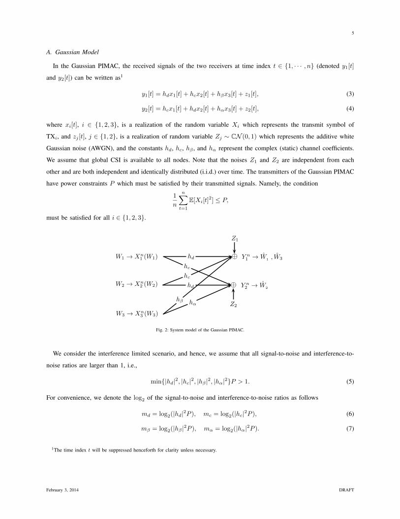
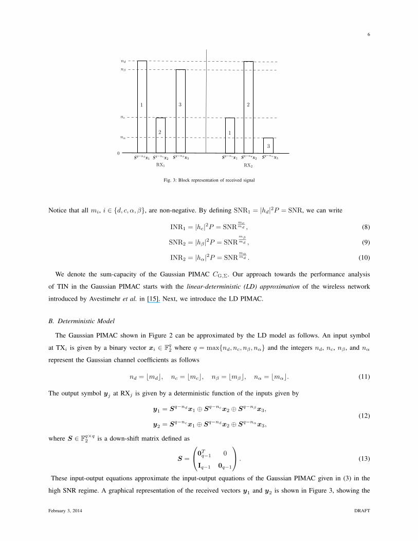
The Gaussian PIMAC shown in Figure 2 can be approximated by the LD model as follows. An input symbol

at TXi is given by a binary vector xi ∈ Fq2 where q = max{nd, nc, nβ , nα} and the integers nd, nc, nβ , and nα

represent the Gaussian channel coefficients as follows

nd = bmdc, nc = bmcc, nβ = bmβc, nα = bmαc. (11)

The output symbol yj at RXj is given by a deterministic function of the inputs given by

y1 = Sq−ndx1 ⊕ Sq−ncx2 ⊕ Sq−nβx3,

y2 = Sq−ncx1 ⊕ Sq−ndx2 ⊕ Sq−nαx3,(12)

where S ∈ Fq×q2 is a down-shift matrix defined as

S =

0Tq−1 0

Iq−1 0q−1

. (13)

These input-output equations approximate the input-output equations of the Gaussian PIMAC given in (3) in the

high SNR regime. A graphical representation of the received vectors y1 and y2 is shown in Figure 3, showing the

February 3, 2014 DRAFT

7

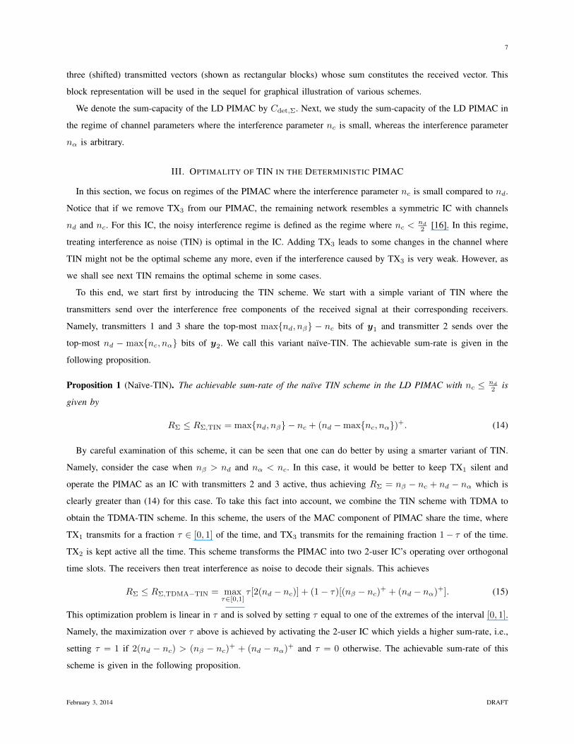
three (shifted) transmitted vectors (shown as rectangular blocks) whose sum constitutes the received vector. This

block representation will be used in the sequel for graphical illustration of various schemes.

We denote the sum-capacity of the LD PIMAC by Cdet,Σ. Next, we study the sum-capacity of the LD PIMAC in

the regime of channel parameters where the interference parameter nc is small, whereas the interference parameter

nα is arbitrary.

III. OPTIMALITY OF TIN IN THE DETERMINISTIC PIMAC

In this section, we focus on regimes of the PIMAC where the interference parameter nc is small compared to nd.

Notice that if we remove TX3 from our PIMAC, the remaining network resembles a symmetric IC with channels

nd and nc. For this IC, the noisy interference regime is defined as the regime where nc < nd2 [16]. In this regime,

treating interference as noise (TIN) is optimal in the IC. Adding TX3 leads to some changes in the channel where

TIN might not be the optimal scheme any more, even if the interference caused by TX3 is very weak. However, as

we shall see next TIN remains the optimal scheme in some cases.

To this end, we start first by introducing the TIN scheme. We start with a simple variant of TIN where the

transmitters send over the interference free components of the received signal at their corresponding receivers.

Namely, transmitters 1 and 3 share the top-most max{nd, nβ} − nc bits of y1 and transmitter 2 sends over the

top-most nd − max{nc, nα} bits of y2. We call this variant naïve-TIN. The achievable sum-rate is given in the

following proposition.

Proposition 1 (Naïve-TIN). The achievable sum-rate of the naïve TIN scheme in the LD PIMAC with nc ≤ nd2 is

given by

RΣ ≤ RΣ,TIN = max{nd, nβ} − nc + (nd −max{nc, nα})+. (14)

By careful examination of this scheme, it can be seen that one can do better by using a smarter variant of TIN.

Namely, consider the case when nβ > nd and nα < nc. In this case, it would be better to keep TX1 silent and

operate the PIMAC as an IC with transmitters 2 and 3 active, thus achieving RΣ = nβ − nc + nd − nα which is

clearly greater than (14) for this case. To take this fact into account, we combine the TIN scheme with TDMA to

obtain the TDMA-TIN scheme. In this scheme, the users of the MAC component of PIMAC share the time, where

TX1 transmits for a fraction τ ∈ [0, 1] of the time, and TX3 transmits for the remaining fraction 1− τ of the time.

TX2 is kept active all the time. This scheme transforms the PIMAC into two 2-user IC’s operating over orthogonal

time slots. The receivers then treat interference as noise to decode their signals. This achieves

RΣ ≤ RΣ,TDMA−TIN = maxτ∈[0,1]

τ [2(nd − nc)] + (1− τ)[(nβ − nc)+ + (nd − nα)+]. (15)

This optimization problem is linear in τ and is solved by setting τ equal to one of the extremes of the interval [0, 1].

Namely, the maximization over τ above is achieved by activating the 2-user IC which yields a higher sum-rate, i.e.,

setting τ = 1 if 2(nd − nc) > (nβ − nc)+ + (nd − nα)+ and τ = 0 otherwise. The achievable sum-rate of this

scheme is given in the following proposition.

February 3, 2014 DRAFT

8

Proposition 2 (TDMA TIN). The achievable sum-rate of the TDMA-TIN scheme in the LD PIMAC with nc ≤ nd2

is given by

RΣ ≤ RΣ,TDMA−TIN = max{2(nd − nc), (nβ − nc)+ + (nd − nα)+}. (16)

For some special cases of the LD PIMAC (specific ranges of the parameters nd, nc, nβ , and nα), the TIN schemes

above can achieve the sum-capacity as we shall show next. Before, we proceed, we divide the parameter space of

the LD PIMAC into several regimes as given in the following definition.

Definition 1. For an LD PIMAC with nc ≤ nd2 , define regimes 1 to 9 as follows:

• Regime 1: nβ ≤ nd − nc and nα > nc,

• Regime 2: nβ ≤ nd − nc and nα ≤ nc,• Regime 3: nβ > nd − nc ≥ nα and nβ − nα ≤ nd − 2nc,

• Regime 4: nβ − nα ≥ nd and nc < nα ≤ nd − nc,• Regime 5: nβ − nα ≥ nd and nα ≤ nc,• Regime 6: nβ − 2nα ≥ nd − nc and nβ − nα < nd,

• Regime 7: nβ > nd − nc and nα > nd − nc,• Regime 8: nα ≤ nd − nc ≤ nβ − nα < nd and nβ − 2nα < nd − nc,• Regime 9: nβ > nd − nc ≥ nα and nd − 2nc < nβ − nα < nd − nc.

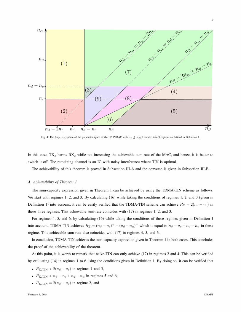
Figure 4 shows the (nβ , nα)-plane of the parameter space for an LD PIMAC with nc ≤ nd2 divided into the

regimes given in Definition 1. In what follows, we study the optimality of TIN over these sub-regimes.

Remark 1. We exclude the special case nβ − nα = nd − nc from our analysis for the following reason: In this

special case, the PIMAC can be modelled as an IC with inputs x1 = Sq−ndx1 ⊕ Sq−nβx3 and x2 and outputs

y1 = x1 ⊕ Sq−ncx2 and y2 = Snd−nc x1 ⊕ Sq−ndx2. The channel can then be treated similar to the IC. We

exclude this case to focus on the specifics of the PIMAC.

Next, we show that TIN is sum-capacity optimal in regimes 1 to 6, but strictly suboptimal in regimes 7 to 9. The

following theorem characterizes the sum-capacity of the LD PIMAC in regimes where TIN is optimal.

Theorem 1. The sum-capacity of the LD PIMAC in regimes 1 to 6 in Fig. 4 is given by

Cdet,Σ =

2(nd − nc), regimes 1, 2, and 3

nβ − nα + nd − nc, regimes 4, 5, and 6.(17)

This theorem shows that TDMA-TIN is sum-capacity optimal in regimes 1 to 6. The performance of TDMA-TIN

and naïve TIN is the same in regimes 2 and 4, and hence, naïve TIN is sum-capacity optimal in these two regimes.

Interestingly, we can notice that TDMA-TIN is optimal in case one MAC transmitter causes noisy interference

nc ≤ nd2 , and the other causes strong interference nα > max{nd, nβ}. This can be seen in regime 1. The intuition

here is that TX3 in this case causes strong interference to RX2, but has a weak channel to its desired receiver RX1.

February 3, 2014 DRAFT

9

Fig. 4: The (nβ , nα)-plane of the parameter space of the LD PIMAC with nc ≤ nd/2 divided into 9 regimes as defined in Definition 1.

In this case, TX3 harms RX2 while not increasing the achievable sum-rate of the MAC, and hence, it is better to

switch it off. The remaining channel is an IC with noisy interference where TIN is optimal.

The achievability of this theorem is proved in Subsection III-A and the converse is given in Subsection III-B.

A. Achievability of Theorem 1

The sum-capacity expression given in Theorem 1 can be achieved by using the TDMA-TIN scheme as follows.

We start with regimes 1, 2, and 3. By calculating (16) while taking the conditions of regimes 1, 2, and 3 (given in

Definition 1) into account, it can be easily verified that the TDMA-TIN scheme can achieve RΣ = 2(nd − nc) in

these three regimes. This achievable sum-rate coincides with (17) in regimes 1, 2, and 3.

For regimes 4, 5, and 6, by calculating (16) while taking the conditions of these regimes given in Definition 1

into account, TDMA-TIN achieves RΣ = (nβ − nc)+ + (nd − nα)+ which is equal to nβ − nc + nd − nα in these

regime. This achievable sum-rate also coincides with (17) in regimes 4, 5, and 6.

In conclusion, TDMA-TIN achieves the sum-capacity expression given in Theorem 1 in both cases. This concludes

the proof of the achievability of the theorem.

At this point, it is worth to remark that naïve-TIN can only achieve (17) in regimes 2 and 4. This can be verified

by evaluating (14) in regimes 1 to 6 using the conditions given in Definition 1. By doing so, it can be verified that

• RΣ,TIN < 2(nd − nc) in regimes 1 and 3,

• RΣ,TIN < nβ − nc + nd − nα in regimes 5 and 6,

• RΣ,TIN = 2(nd − nc) in regime 2, and

February 3, 2014 DRAFT

10

• RΣ,TIN = nβ − nc + nd − nα in regime 4.

This shows the inferiority of this naïve TIN scheme in comparison to the smarter TDMA-TIN which is sum-

capacity optimal for a wider range of channel parameters.

B. Converse of Theorem 1

The converse of Theorem 1 is based on the three lemmas that we provide next. The main idea of the following

lemmas is reducing the PIMAC by removing one interferer at RX2 into a channel that can be treated similar to the

IC.

Lemma 1. The sum-capacity of the LD PIMAC is upper bounded as follow

Cdet,Σ ≤ max{nd − nc, nc, nβ}+ max{nd − nc, nc}. (18)

Proof: The idea of the proof is to create a genie-aided channel where each receiver experiences one and only

one interference just as in the IC. By doing this, the resulting channel can be treated in a similar way as the IC

[16], and the given bound can be obtained. To this end, we give W3 to RX2 as side information. This enhances

the PIMAC to a channel where RX1 experiences interference from x2 and RX2 experiences interference from x1

only. Next, we treat the resulting enhanced channel as an IC and derive a bound similar to that of the IC with noisy

interference. Namely, we give the interference caused by TX1 given by Sq−ncxn1 to RX1 as side information, and

we give the interference caused by TX2 given by Sq−ncxn2 to RX2 as side information. The resulting PIMAC which

has been enhanced with side information is more capable than the original PIMAC, and hence the capacity of the

former serves as an upper bound for the capacity of the latter. Next, by using Fano’s inequality we can bound RΣ

as follows2

n(RΣ − εn) ≤ I(W1,W3;yn1 ,Sq−ncxn1 ) + I(W2;yn2 ,S

q−ncxn2 ,W3), (19)

where εn → 0 as n→∞. By using the chain rule, and the independence of the different messages, we can rewrite

this bound as

n(RΣ − εn) ≤ I(W1,W3;Sq−ncxn1 ) + I(W1,W3;yn1 |Sq−ncxn1 )

+ I(W2;Sq−ncxn2 |W3) + I(W2;yn2 |Sq−ncxn2 ,W3). (20)

Now we treat each of the mutual information terms in (20) separately. The first mutual information term can be

written as

I(W1,W3;Sq−ncxn1 ) = H(Sq−ncxn1 )−H(Sq−ncxn1 |W1,W3)

= H(Sq−ncxn1 ), (21)

2We abuse the notation by using x and y to denote random vectors.

February 3, 2014 DRAFT

11

since H(Sq−ncxn1 |W1,W3) = 0. The second mutual information term in (20) satisfies

I(W1,W3;yn1 |Sq−ncxn1 ) = H(yn1 |Sq−ncxn1 )−H(yn1 |Sq−ncxn1 ,W1,W3)

= H(yn1 |Sq−ncxn1 )−H(Sq−ncxn2 ), (22)

since given W1 and W3, the only randomness remaining in y1 is that of x2. The third mutual information term in

(20) satisfies

I(W2;Sq−ncxn2 |W3) = H(Sq−ncxn2 |W3)−H(Sq−ncxn2 |W2,W3)

= H(Sq−ncxn2 ) (23)

which follows since H(Sq−ncxn2 |W2,W3) = 0 and since x2 is independent of W3. Finally, the last mutual

information term in (20) satisfies

I(W2;yn2 |Sq−ncxn2 ,W3) = H(yn2 |Sq−ncxn2 ,W3)−H(yn2 |Sq−ncxn2 ,W2,W3)

= H(yn2 |Sq−ncxn2 ,W3)−H(Sq−ncxn1 ) (24)

since given W2 and W3, the only randomness in y2 is that of x1. Now by substituting (21)-(24) in (20), we obtain

n(RΣ − εn) ≤ H(Sq−ncxn1 ) +H(yn1 |Sq−ncxn1 )−H(Sq−ncxn2 ) +H(Sq−ncxn2 )

+H(yn2 |Sq−ncxn2 ,W3)−H(Sq−ncxn1 ) (25)

= H(yn1 |Sq−ncxn1 ) +H(yn2 |Sq−ncxn2 ,W3). (26)

Now notice that given Sq−ncxn1 , the top-most nc components of xn1 are known and can be subtracted from yn1

leaving max{nd − nc, nc, nβ} random components in y1. The entropy of a binary vector is maximized if its

components are i.i.d. with a Bernoulli distribution with probability 1/2, and the maximum entropy is equal to the

length of the vector. This leads to

H(yn1 |Sq−ncxn1 ) =

n∑t=1

H(y1[t]|Sq−ncxn1 ,yt−11 ) (27)

≤n∑t=1

max{nd − nc, nc, nβ} (28)

= nmax{nd − nc, nc, nβ}. (29)

Similarly,

H(yn2 |Sq−ncxn2 ,W3) ≤ nmax{nd − nc, nc}. (30)

Therefore, we can write

n(RΣ − εn) ≤ n(max{nd − nc, nc, nβ}+ max{nd − nc, nc}). (31)

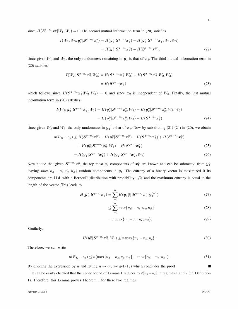
By dividing the expression by n and letting n→∞, we get (18) which concludes the proof.

It can be easily checked that the upper bound of Lemma 1 reduces to 2(nd−nc) in regimes 1 and 2 (cf. Definition

1). Therefore, this Lemma proves Theorem 1 for these two regimes.

February 3, 2014 DRAFT

12

The following is another upper bound on the sum-rate of the LD PIMAC obtained by removing the interference

from TX1 to RX2, i.e., giving W1 to RX2 as side information.

Lemma 2. The sum-capacity of the LD PIMAC is upper bounded as follows

Cdet,Σ ≤ max{nd, nc, nβ − nα}+ max{nd − nc, nα}. (32)

Proof: The proof of this lemma is similar to that of Lemma 1 where instead of W3, we give W1 to RX2 as

side information. Then, the resulting IC is treated similarly, and the desired upper bound is obtained. The details

are given in Appendix A.

By examining this upper bound and using the definitions of regimes 4 and 5 given in Definition 1, it can be

easily verified that the upper bound of Lemma 2 reduces to nβ − nc + nd − nα in regimes 4 and 5. Therefore, this

Lemma proves Theorem 1 for these two regimes.

It remains to prove Theorem 1 for regimes 3 and 6. For this purpose we need two new upper bounds derived

specifically for these two regimes. These bounds are given in the following lemma.

Lemma 3. The sum-capacity of the LD PIMAC with nc ≤ nd2 is upper bounded by

Cdet,Σ ≤ 2(nd − nc) in regime 3 (33)

Cdet,Σ ≤ nβ − nα + nd − nc in regime 6. (34)

Proof: We start by considering a sub-regime of regime 6 defined by

nβ − 2nα > nd − nc, nβ − nα < nd, nβ < nd. (35)

Then we use Fano’s inequality to write

n(RΣ − εn) ≤ I(xn1 ,xn3 ;yn1 ) + I(xn2 ;yn2 )

= H(yn1 )−H(yn1 |xn1 ,xn3 ) +H(yn2 )−H(yn2 |xn2 ) (36)

where εn → 0 as n→∞. Using the chain rule and dropping conditions, the first term can be upper bounded by

H(yn1 ) ≤ H(xn1,1,xn1,2 ⊕ xn3,1) +H

(yn1,[nd−nβ+nα+1:nd]

), (37)

where

xn1,1 = xn1,[1:nd−nβ ], xn1,2 = xn1,[nd−nβ+1:nd−nβ+nα], and xn3,1 = xn3,[1:nα], (38)

and where the first entropy term in (37) does not have any contribution from x2 since nβ − nα > nc from (35).

The third entropy term in (36) can be upper bounded by

H(yn2 ) ≤ H(xn2,[1:nc]

)+H

(yn2,[nc+1:nd]

), (39)

where the first entropy term in (40) does not have any contribution from x1 and x3 since nc < nd − nc and

nc < nd − nα (cf. (35)). For the second entropy term in (36), we have

−H(yn1 |xn1 ,xn3 ) = −H(Sq−ncxn2 ) = −H(xn2,[1:nc]

). (40)

February 3, 2014 DRAFT

13

Finally, for the fourth entropy term in (40), we write

−H(yn2 |xn2 ) = −H(yn2 ⊕ Sq−ndxn2 |xn2 ) = −H(Sq−ncxn1 ⊕ Sq−nαxn3 ) (41)

= −H(xn1,1,xn1,2,x

n1,3,x

n1,4 ⊕ xn3,1) (42)

where xn1,1, xn1,2, and xn3,1 are defined in (38), and xn1,3 = xn1,[nd−nβ+nα+1:nc−nα] and xn1,4 = xn1,[nc−nα+1:nc].

Next, we use the chain rule to write

−H(yn2 |xn2 ) = −H(xn1,1,xn1,2,x

n1,4 ⊕ xn3,1)−H(xn1,3|xn1,1,xn1,2,xn1,4 ⊕ xn3,1)

≤ −H(xn1,1,xn1,2,x

n1,4 ⊕ xn3,1) (43)

Substituting (37), (39), (40), and (43) in (36) yields

n(RΣ − εn) ≤ H(xn1,1,xn1,2 ⊕ xn3,1)−H(xn1,1,x

n1,2,x

n1,4 ⊕ xn3,1)

+H(yn1,[nd−nβ+nα+1:nd]

)+H

(yn2,[nc+1:nd]

)(44)

Using Lemma 4 given in Appendix B, the first two terms above can be upper bounded by 0, and (44) can be upper

bounded by

n(RΣ − εn) ≤ H(yn1,[nd−nβ+nα+1:nd]

)+H

(yn2,[nc+1:nd]

)≤ n(nβ − nα + nd − nc) (45)

by maximizing the entropy terms using the i.i.d. Bernoulli distribution with probability 1/2. So, by dividing by n

and letting n→∞, εn → 0 and the sum rate in this regime can be bounded as

RΣ ≤ nβ − nα + nd − nc, (46)

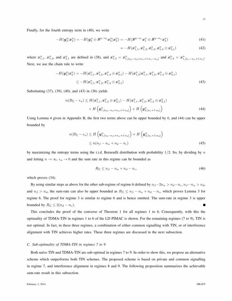
which proves (34).

By using similar steps as above for the other sub-regime of regime 6 defined by nβ−2nα > nd−nc, nβ−nα > nd,

and nβ > nd, the sum-rate can also be upper bounded as RΣ ≤ nβ − nα + nd − nc, which proves Lemma 3 for

regime 6. The proof for regime 3 is similar to regime 6 and is hence omitted. The sum-rate in regime 3 is upper

bounded by RΣ ≤ 2(nd − nc).

This concludes the proof of the converse of Theorem 1 for all regimes 1 to 6. Consequently, with this the

optimality of TDMA-TIN in regimes 1 to 6 of the LD PIMAC is shown. For the remaining regimes (7 to 9), TIN is

not optimal. In fact, in these three regimes, a combination of either common signalling with TIN, or of interference

alignment with TIN achieves higher rates. These three regimes are discussed in the next subsection.

C. Sub-optimality of TDMA-TIN in regimes 7 to 9

Both naïve TIN and TDMA-TIN are sub-optimal in regimes 7 to 9. In order to show this, we propose an alternative

scheme which outperforms both TIN schemes. The proposed scheme is based on private and common signalling

in regime 7, and interference alignment in regimes 8 and 9. The following proposition summarizes the achievable

sum-rate result in this subsection.

February 3, 2014 DRAFT

14

Proposition 3. The following sum-rate is achievable in a PIMAC with nc ≤ nd2

RΣ,c = max{min{nα, nβ}+ nd − nc, nβ} regime 7 (47)

RΣ,a = (nd − nc) + min{

2µ− ν, nd − (nc − nα)+, nβ − (nα − nc)+}

regimes 8 and 9 (48)

where µ = max{nβ − nα, nd − nc} and ν = min{nβ − nα, nd − nc}.

Now we describe the schemes that achieve the sum-rate given in this proposition. We start with regime 7 by

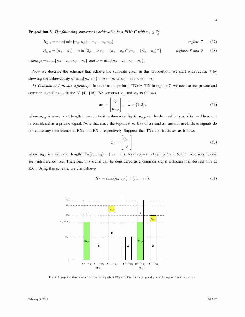
showing the achievability of min{nα, nβ}+ nd − nc if nβ − nα < nd − nc.1) Common and private signalling: In order to outperform TDMA-TIN in regime 7, we need to use private and

common signalling as in the IC [4], [16]. We construct x1 and x2 as follows

xk =

0

uk,p

, k ∈ {1, 2}, (49)

where uk,p is a vector of length nd−nc. As it is shown in Fig. 6, uk,p can be decoded only at RXk, and hence, it

is considered as a private signal. Note that since the top-most nc bits of x1 and x2 are not used, these signals do

not cause any interference at RX2 and RX1, respectively. Suppose that TX3 constructs x3 as follows

x3 =

u3,c

0

, (50)

where u3,c is a vector of length min{nα, nβ} − (nd − nc). As it shown in Figures 5 and 6, both receivers receive

u3,c interference free. Therefore, this signal can be considered as a common signal although it is desired only at

RX1. Using this scheme, we can achieve

RΣ = min{nα, nβ}+ (nd − nc). (51)

nd

nβ

nα

nd − nc

nc

Sq−ndx1 Sq−ncx2 Sq−nβx3 Sq−ncx1 Sq−ndx2 Sq−nαx3RX1 RX2

0

0

0 0 0

0

u1,p

u3,c

u2,p

u3,c

0

Fig. 5: A graphical illustration of the received signals at RX1 and RX2 for the proposed scheme for regime 7 with nα < nβ .

February 3, 2014 DRAFT

15

nd

nβ

nα

nd − nc

nc

Sq−ndx1 Sq−ncx2 Sq−nβx3 Sq−ncx1 Sq−ndx2 Sq−nαx3

RX1 RX2

0

0 0 0

0

0u1,p u2,p

u3,c

u3,c

0

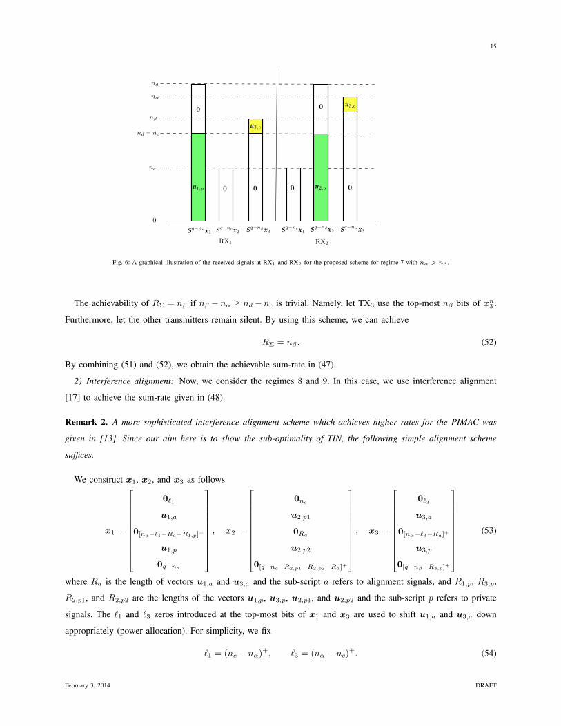
Fig. 6: A graphical illustration of the received signals at RX1 and RX2 for the proposed scheme for regime 7 with nα > nβ .

The achievability of RΣ = nβ if nβ − nα ≥ nd − nc is trivial. Namely, let TX3 use the top-most nβ bits of xn3 .

Furthermore, let the other transmitters remain silent. By using this scheme, we can achieve

RΣ = nβ . (52)

By combining (51) and (52), we obtain the achievable sum-rate in (47).

2) Interference alignment: Now, we consider the regimes 8 and 9. In this case, we use interference alignment

[17] to achieve the sum-rate given in (48).

Remark 2. A more sophisticated interference alignment scheme which achieves higher rates for the PIMAC was

given in [13]. Since our aim here is to show the sub-optimality of TIN, the following simple alignment scheme

suffices.

We construct x1, x2, and x3 as follows

x1 =

0`1

u1,a

0[nd−`1−Ra−R1,p]+

u1,p

0q−nd

, x2 =

0nc

u2,p1

0Ra

u2,p2

0[q−nc−R2,p1−R2,p2−Ra]+

, x3 =

0`3

u3,a

0[nα−`3−Ra]+

u3,p

0[q−nβ−R3,p]+

(53)

where Ra is the length of vectors u1,a and u3,a and the sub-script a refers to alignment signals, and R1,p, R3,p,

R2,p1, and R2,p2 are the lengths of the vectors u1,p, u3,p, u2,p1, and u2,p2 and the sub-script p refers to private

signals. The `1 and `3 zeros introduced at the top-most bits of x1 and x3 are used to shift u1,a and u3,a down

appropriately (power allocation). For simplicity, we fix

`1 = (nc − nα)+, `3 = (nα − nc)+. (54)

February 3, 2014 DRAFT

16

nd

nd − nc

nc

nα

nβ

nβ − nα

nd − ℓ1

0

0

0 0

0

0

0

0

0 ℓ1

Ra

ℓ1

nα −Ra

u1,a

u3,a

u1,a u3,a

0

Sq−ndx1 Sq−ncx2 Sq−nβx3 Sq−ncx1 Sq−ndx2 Sq−nαx3

RX1 RX2

u1,p

u3,p

u2,p1

u2,p2

0

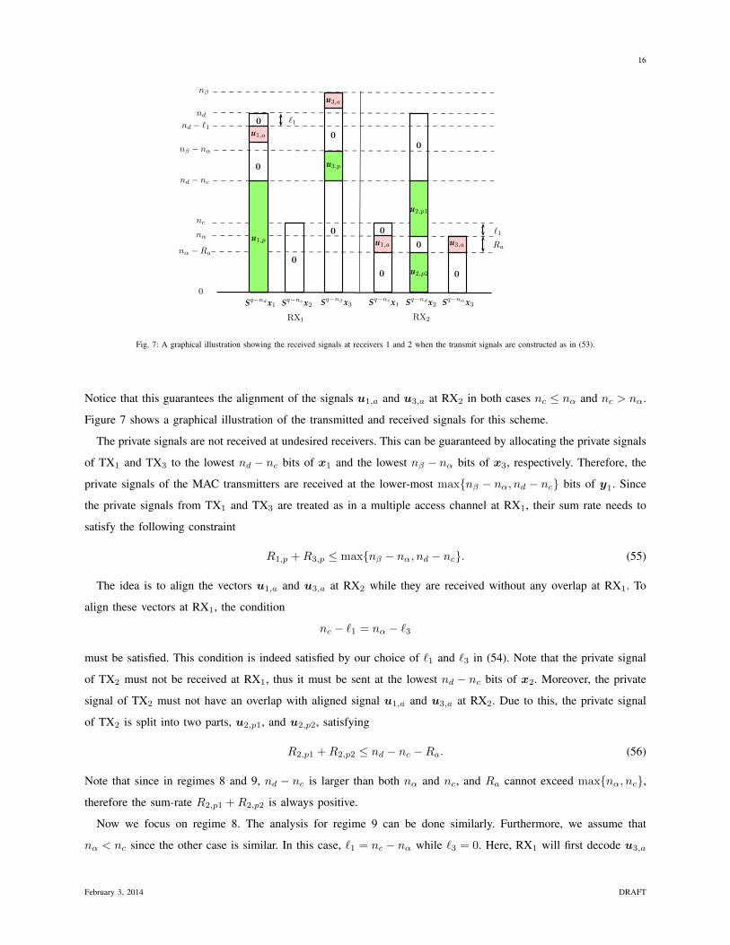
Fig. 7: A graphical illustration showing the received signals at receivers 1 and 2 when the transmit signals are constructed as in (53).

Notice that this guarantees the alignment of the signals u1,a and u3,a at RX2 in both cases nc ≤ nα and nc > nα.

Figure 7 shows a graphical illustration of the transmitted and received signals for this scheme.

The private signals are not received at undesired receivers. This can be guaranteed by allocating the private signals

of TX1 and TX3 to the lowest nd − nc bits of x1 and the lowest nβ − nα bits of x3, respectively. Therefore, the

private signals of the MAC transmitters are received at the lower-most max{nβ − nα, nd − nc} bits of y1. Since

the private signals from TX1 and TX3 are treated as in a multiple access channel at RX1, their sum rate needs to

satisfy the following constraint

R1,p +R3,p ≤ max{nβ − nα, nd − nc}. (55)

The idea is to align the vectors u1,a and u3,a at RX2 while they are received without any overlap at RX1. To

align these vectors at RX1, the condition

nc − `1 = nα − `3

must be satisfied. This condition is indeed satisfied by our choice of `1 and `3 in (54). Note that the private signal

of TX2 must not be received at RX1, thus it must be sent at the lowest nd − nc bits of x2. Moreover, the private

signal of TX2 must not have an overlap with aligned signal u1,a and u3,a at RX2. Due to this, the private signal

of TX2 is split into two parts, u2,p1, and u2,p2, satisfying

R2,p1 +R2,p2 ≤ nd − nc −Ra. (56)

Note that since in regimes 8 and 9, nd − nc is larger than both nα and nc, and Ra cannot exceed max{nα, nc},therefore the sum-rate R2,p1 +R2,p2 is always positive.

Now we focus on regime 8. The analysis for regime 9 can be done similarly. Furthermore, we assume that

nα < nc since the other case is similar. In this case, `1 = nc − nα while `3 = 0. Here, RX1 will first decode u3,a

February 3, 2014 DRAFT

17

and then u1,a. Thus, we obtain the following condition

Ra ≤ (nβ − nd)+ + `1. (57)

Substituting `1 = nc − nα into (57), we get

Ra ≤

nβ − nα − nd + nc if nd ≤ nβ

nc − nα if nβ < nd.

Note that in second case where nβ < nd, the expression nβ − nα − nd + nc is smaller than nc − nα. Therefore,

the following rate for Ra is also achievable

Ra ≤ nβ − nα − nd + nc. (58)

In addition to this, vector u1,a must not have any overlap with private vectors u1,p and u3,a. Due to this, the

following condition has to be satisfied

Ra ≤ nd − `1 −max{nβ − nα, nd − nc}.︸ ︷︷ ︸R1,p+R3,p

(59)

Considering the conditions of regime 8, and substituting `1 = nc − nα, we obtain

Ra ≤ nd − nc − nβ + 2nα. (60)

Note that the expression nd − nc − nβ + 2nα = 0 represents the border line of regime 8 when nα < nc. As shown

in Fig. 4, the right-hand side of the inequality in (60) is positive in this regime. Combining the conditions in (58)

and (59), we will get

Ra ≤ min{nβ − nα − nd + nc, nd − `1 − (R1,p +R3,p)}. (61)

This is the rate of the alignment message in regime 8 with nc > nα. For the other case where nc < nα, we can

show that the same rate given in (61) is achievable for the alignment messages. Note that in this case `1 = 0 and

`3 = nα − nc.The presented transmission scheme for regime 8 can be extended for regime 9 as well, with a slight difference,

namely in the order of decoding u1,a and u3,a at RX1. The decoding order of these signals is opposite to the one

used in regime 8. Consequently, the condition on Ra will be different in regime 9 than (61), but can be calculated

similarly.

The following is the achievable rate for the alignment messages for both regimes 8 and 9 combined

Ra ≤ min {|nβ − nα − nd + nc|, nd − `1 −R1,p −R3,p, nβ − `3 −R1,p −R3,p} . (62)

For both regimes 8 and 9 (excluding the case where nβ − nα = nd − nc discussed in Remark 1), we can show

that the right-hand side of (62) is positive (cf. Definition 1). By adding the achievable rates of the private messages

(55) and (56) and that of the alignment messages (62), and substituting the values of `1 and `3, we conclude that

the sum-rate given by

RΣ ≤ (nd − nc) + min{

2µ− ν, nd − (nc − nα)+, nβ − (nα − nc)+}, (63)

February 3, 2014 DRAFT

18

is achievable, where µ = max{nβ − nα, nd − nc} and ν = min{nβ − nα, nd − nc}. This proves the achievability

of (48) in Proposition 3

3) Comparison with TDMA-TIN: The achievable rates provided in Proposition 3 are larger than the rates achiev-

able using TIN. Namely, for regime 7, TDMA-TIN achieves

RΣ,TDMA−TIN = max{2(nd − nc), (nβ − nc)+ + (nd − nα)+} (64)

= max{2(nd − nc), nβ − nc + (nd − nα)+} (65)

< max{2(nd − nc), nβ} (66)

< max{min{nα, nβ}+ nd − nc, nβ}, (67)

where the first inequality follows since −nc + (nd − nα)+ = −nc + max{0, nd − nα} < 0 since nα > nd − ncin regime 7, and the second inequality follows since both nα and nβ are greater than nd − nc in this regime. Note

that (67) is the achievable rate given in Proposition 3 in regime 7, and therefore, the proposed scheme outperforms

TDMA-TIN and consequently, naïve TIN in this regime.

Considering the definition of regimes 8 and 9, in these regimes, RΣ,TDMA-TIN = (nd−nc)+max{nβ−nα, nd−nc}.In regimes 8 and 9, the achievable rate of the alignment scheme is

RΣ = (nd − nc) + min{

2µ− ν, nd − (nc − nα)+, nβ − (nα − nc)+}, (68)

where µ = max{nβ − nα, nd − nc} and ν = min{nβ − nα, nd − nc}. This can be rewritten as

RΣ = (nd − nc) + µ+ min{µ− ν, nd − (nc − nα)+ − µ, nβ − (nα − nc)+ − µ

}(69)

= RΣ,TDMA−TIN + min{µ− ν, nd − (nc − nα)+ − µ, nβ − (nα − nc)+ − µ

}, (70)

which is larger than RΣ,TDMA−TIN since, as mentioned in proof of Proposition 3, the min expression above is

non-negative. Thus, the alignment scheme outperforms both TDMA-TIN and naïve TIN in both regimes 8 and 9.

In conclusion, combining TIN with common signalling (regime 7) and with interference alignment (regimes 8

and 9) leads to a better performance than using plain TIN. This conclusion is particularly interesting in regimes

where both receivers experience ‘very-weak’ interference in the sense that the interference parameter is smaller than

half the desired channel parameter, i.e.,

nc ≤ max{nd

2,nβ2

}(71)

max{nc, nα} ≤nd2. (72)

While the first condition is guaranteed by our consideration of nc ≤ nd2 , the second condition is not guaranteed.

If the second condition holds, then both receivers have interference that is weaker than half their desired channel

(very-weak interference). In this case, one would expect that TIN is optimal. However, even in this case it can

occur that IA is better than TIN although the channel satisfies (71). For instance, if (nd, nc, nβ , nα) = (5, 2, 6, 2),

then while conditions (71) and (72) are satisfied, the channel is in regime 8 where combining TIN with IA is better

than using TDMA-TIN. Interestingly, the given example is also noisy according to [9] where the noisy interference

February 3, 2014 DRAFT

19

regime of the IC is defined as the case where the desired signal of each user is stronger than the sum of the strongest

interference it receives and the strongest interference it causes3. If we apply this condition to the PIMAC in this

example, we can see that the sum of the strongest produced and received interference is nc + max{nc, nα} = 4

which is smaller than both direct channel parameters nd and nβ , but still TIN is sub-optimal.

IV. EXTENSION TO THE GAUSSIAN PIMAC

For the linear deterministic PIMAC, we have shown that the naïve TIN scheme is optimal only in regimes 2 and

4 and TDMA-TIN in regimes 1-6. In this section, we assess the optimality of naïve TIN and TDMA-TIN in the

Gaussian case by finding the gap between the upper bound and the achievable sum-rates in the regimes where this

gap can be upper bounded by a constant. Note that in the Gaussian case, the regimes are defined similar to the

deterministic case, with ni replaced by mi for i ∈ {d, c, α, γ}. Using the insights from linear deterministic PIMAC,

we establish the upper bounds for the Gaussian case, as follows.

Theorem 2. The sum-capacity of the Gaussian PIMAC is upper bounded by

CG,Σ ≤ log2

(1 + SNR

mcmd + SNR

mβmd +

SNR

1 + SNRmcmd

)+ log

(1 + SNR

mcmd +

SNR

1 + SNRmcmd

)(73)

CG,Σ ≤ log2

(1 + SNR + SNR

mcmd +

SNRmβmd

1 + SNRmαmd

)+ log

(1 + SNR

mαmd +

SNR

1 + SNRmcmd

)(74)

Proof: The proof for these two upper bounds is essentially similar to the proofs of Lemmas 1 and 2, but with

some steps in the proof adapted to the Gaussian PIMAC. Details can be found in Appendix C.

The naïve TIN scheme achieves these bounds within a constant gap in regimes 2 and 4. This is shown in the

next subsection.

A. Naïve TIN is optimal within a constant gap in regimes 2 and 4

In naïve TIN, all transmitters send with the full power. This causes interference at undesired receivers. At the

receiver side, the strategy is the same as if there were no interference. Therefore, the receivers decode their desired

signals while the interference is treated as noise. Hence, RX1 decodes W1 and W3 as in a multiple access channel

(successive decoding) with noise variance 1 + |hc|2P , and RX2 decodes W2 as in a point-to-point channel with

noise variance 1 + |hc|2P + |hα|2P . Hence, we obtain the following result.

Proposition 4. The achievable sum-rate of the naïve-TIN in the Gaussian PIMAC is given by

RΣ,TIN ≤ log2

(1 +

SNR + SNRmβmd

1 + SNRmcmd

)+ log2

(1 +

SNR

1 + SNRmcmd + SNR

mαmd

). (75)

By comparing the achievable sum rate in (75) with the upper bounds in (73) and (74), we can show that naïve

TIN can achieve the sum-capacity within a constant gap in regimes 2 and 4 (where naïve TIN is optimal for the

LD PIMAC). The following corollary summarizes this result.

3It does not follow from [9] that the same TIN optimality condition has to hold of the PIMAC.

February 3, 2014 DRAFT

20

Corollary 1. The achievable sum-rate of naïve-TIN is within a gap of 3 + 2 log2 3 bits of the sum-capacity of the

Gaussian PIMAC in regimes 2 and 4.

Proof: The gap calculation is given in Appendix D.

TDMA-TIN is also optimal within a constant gap in these two regimes. In fact, TDMA-TIN outperforms TIN as

we show next.

B. TDMA-TIN strictly outperforms naïve TIN

In contrast to naïve-TIN, in TDMA-TIN not all transmitters are active at the same time. The transmitting scheme

for TDMA-TIN is as follows. TX1 sends X1 ∼ CN (0, Pτ ), where τ denotes the portion of time τ ∈ [0, 1] in which

TX1 is active. In the remaining (1− τ) fraction of time, TX3 transmits X3 ∼ CN (0, P1−τ ). Note that TX2 is active

all the time and its transmit signal is X2 ∼ CN (0, P ). The achievable sum-rate by using TDMA-TIN is presented

in the following proposition.

Proposition 5. The achievable sum-rate of TDMA-TIN in the Gaussian PIMAC is given by

RΣ,TDMA−TIN ≤ maxτ∈[0,1]

τlog2

1 +

SNR

τ

1 + SNRmcmd

+ log2

1 +SNR

1 +SNR

mcmd

τ

+ (1− τ)

log2

1 +

SNRmβmd

1− τ1 + SNR

mcmd

+ log2

1 +SNR

1 +SNR

mαmd

1− τ

. (76)

As we have seen in the LD PIMAC, TDMA-TIN also outperforms naïve TIN in the Gaussian case. This interesting

statement is given in the following corollary.

Corollary 2. TDMA-TIN strictly outperforms naïve TIN, i.e.,

RΣ,TDMA−TIN > RΣ,TIN

for all values of channel parameters except for the case where |hd||hβ | = |hc||hα| .

Proof: The proof is given in Appendix E. Note that the excluded case corresponds to the special case discussed

in Remark 1 where the PIMAC can be modelled as an IC.

Remark 3. The difference between TDMA-TIN and naïve TIN is that while all transmitters are simultaneously

active in the latter, the same is not true in the former. In TDMA-TIN, one transmitter is switched of, leading to

a larger sum-rate than naïve TIN. A similar behaviour was observed in the K-user IC in [9, Example 2] where

higher rates can be achieved by switching one transmitter off and using TIN at the receivers.

This means that although naïve TIN achieves the sum-capacity of the PIMAC within a constant gap in regimes 2

and 4, it can not be sum-capacity optimal since it is strictly outperformed by TDMA-TIN. Clearly, since naïve TIN

February 3, 2014 DRAFT

21

achieves the sum-capacity of the Gaussian PIMAC within a constant gap in regimes 2 and 4, so does TDMA-TIN.

Additionally, TDMA-TIN also achieves the sum-capacity of the Gaussian PIMAC within a constant gap in regimes

1 and 5 (contrary to naïve TIN which does not). The gap between the achievable sum-rate of TDMA-TIN and the

sum-capacity upper bound is given in the following corollary.

Corollary 3. The achievable sum-rate of TDMA-TIN is within a gap of 4 + log2 3 bits of the sum-capacity of the

Gaussian PIMAC in regimes 1, 2, 4 and 5.

Proof: The proof is given in Appendix F.

Although TDMA-TIN achieves the sum-capacity of the LD PIMAC in regimes 3 and 6, we do not show that it

achieves the sum-capacity within a constant gap in regimes 3 and 6 of the Gaussian PIMAC. The reason is that the

upper bounds derived in Lemma 3 can not be extended to the Gaussian PIMAC, since they are based on Lemma 4

which applies only of the linear deterministic model. However, we claim that TDMA-TIN is also optimal within a

constant gap in these two regimes, i.e., 3 and 6.

C. Sub-optimality of TDMA-TIN in regimes 7 to 9

Although TDMA-TIN always outperforms naïve TIN, it is sub-optimal in regimes 7 to 9. As discussed in Sections

III-C1 and III-C2, a combination of common signalling and private signalling outperforms TDMA-TIN in regime

7, and a combination of interference alignment and TIN outperforms it in regimes 8 and 9. This is also true in the

Gaussian PIMAC at high SNR as we show next. We start by deriving the achievable rate of common and private

signalling. The details of the scheme are given in Appendix G.

Proposition 6. The following sum-rate is achievable in regime 7 of the Gaussian PIMAC with high SNR

RΣ,c =

3∑i=1

(Ri,p +Ri,c) , (77)

where

R1,p ≤ [md + r1,p − (mc + r2,p)+]+, (78)

R2,p ≤ [md + r2,p −max{0,mc + r1,p,mα + r3,p}]+, (79)

R3,p ≤ [mβ + r3,p −max{0,md + r1,p,mc + r2,p}]+, (80)

R1,c ≤ min{

[md + r1,c −max{0,md + r1,p,mc + r2,p,mβ + r3,p}]+,

[mc + r1,c −max{0,mc + r1,p,md + r2,p,md + r2,c,mα + r3,p}]+}

(81)

R2,c ≤ min{

[mc + r2,c −max{0,md + r1,p,md + r1,c,mc + r2,p,mβ + r3,p,mβ + r3,c}]+,

[md + r2,c −max{0,mc + r1,p,md + r2,p,mα + r3,p}]+}, (82)

R3,c ≤ min{

[mβ + r3,c −max{0,md + r1,p,md + r1,c,mc + r2,p,mβ + r3,p}]+

[mα + r3,c −max{0,mc + r1,p,mc + r1,c,md + r2,p,md + r2,c,mα + r3,p}]+}, (83)

February 3, 2014 DRAFT

22

A1 = min{[mc + r1,a −max{0,mc + r1,p,mα + r3,p,md + r2,p2}]+,

[mβ + r3,a −max{0, 2md + r1,p + r1,a,mβ + r3,p, 2mc + r2,p1 + r2,p2}]+,

[md + r1,a −max{0,mβ + r3,p,md + r1,p, 2mc + r2,p1 + r2,p2}]+} (91)

A2 = min{[mc + r1,a −max{0,mc + r1,p,mα + r3,p,md + r2,p2}]+,

[md + r1,a −max{0,md + r1,p, 2mβ + r3,p + r3,a, 2mc + r2,p1 + r2,p2}]+,

[mβ + r3,a −max{0,md + r1,p,mβ + r3,p, 2mc + r2,p1 + r2,p2}]+} (92)

and ri,p, ri,c ≤ 0, 2ri,p + 2ri,c ≤ 1.

The parameters ri,p and ri,c play the role of power allocation parameters, and are defined as log2

(Pi,pP

)and

log2

(Pi,cP

)where Pi,p and Pi,c are the powers of the private and the common signals, respectively. Note that by

varying ri,p (or ri,c) from −∞ to 0, we can vary Pi,p (or Pi,c) from 0 to P . The condition 2ri,p + 2ri,c ≤ 1

guarantees the satisfaction of the power constraint at the transmitters.

The achievable sum-rate of the interference alignment scheme presented in Section III-C2 can be also extended

to the Gaussian PIMAC, leading to the following proposition.

Proposition 7. The following sum-rate is achievable in regimes 8 and 9 of the the Gaussian PIMAC with high SNR

RΣ,a = R1,p + 2Ra +R2,p1 +R2,p2 +R3,p, (84)

where

R1,p ≤ [md + r1,p − (2mc + r2,p1 + r2,p2)+]+ (85)

R3,p ≤ [mβ + r3,p − (2mc + r2,p1 + r2,p2)+]+ (86)

R3,p +R1,p ≤ [max{mβ + r3,p,md + r1,p} − (2mc + r2,p1 + r2,p2)+]+ (87)

R2,p1 ≤ [md + r2,p1 −max{0, 2mc + r1,p + r1,a, 2mα + r3,p + r3,a,md + r2,p2}]+ (88)

R2,p2 ≤ [md + r2,p2 −max{0,mc + r1,p,mα + r3,p}]+ (89)

Ra ≤

A1 if |hβ ||hα| <

|hd||hc|

A2 otherwise(90)

where A1 and A2 are defined in (91) and (92) at the top of the page, and for i ∈ {1, 3}, ri,p, ri,a, r2,p1, r2,p2 ≤ 0,

and 2r1,p + 2r1,a ≤ 1, 2r3,p + 2r3,a ≤ 1, 2r2,p1 + 2r2,p2 ≤ 1.

The details of the scheme are given in Appendix H. By varying the power allocation parameters (r’s) of these

schemes, different rates can be achieved. In order to obtain the highest acheivable sum-rates of these schemes, one

February 3, 2014 DRAFT

23

has to optimize over the various power allocations. Next, we show that there exists power allocations that lead to

higher achievable sum-rates than that of TDMA-TIN in regimes 7 to 9.

Corollary 4. The achievable sum-rate of TDMA-TIN is not within a constant gap of the sum-capacity of the Gaussian

PIMAC in regimes 7, 8, and 9.

To prove this corollary, we need to find power allocations for the rates in Propositions 6 and 7 that outperform

TDMA-TIN at high SNR. We start by identifying the achievable sum-rate of TDMA-TIN at high SNR in regimes

7-9.

RΣ,TDMA−TIN ≈ maxτ∈[0,1]

{τ

[log2

(1 +

SNR

τSNRmcmd

)+ log2

(1 +

τSNR

SNRmcmd

)]

(1− τ)

[log2

(1 +

SNRmβmd

(1− τ)SNRmcmd

)+ log2

(1 +

(1− τ)SNR

SNRmαmd

)]}(a)≈ max

τ∈[0,1]

{τ

[log2

(SNR

τSNRmcmd

)+ log2

(τSNR

SNRmcmd

)]

(1− τ)

[log2

(SNR

mβmd

(1− τ)SNRmcmd

)+ log2

((1− τ)SNR

SNRmαmd

)]}

= maxτ∈[0,1]

{τ [2(md −mc)] + (1− τ)[mβ −mc + (md −mα)+]}. (93)

Note that (a) is due to the fact that in regimes 7 to 9, both mβ and md are larger than mc, and in the high SNR

regime, SNRmd−mcmd ,SNR

mβ−mcmd � 1. Therefore, the achievable rate of TDMA-TIN can be approximated as

RΣ,TDMA−TIN = maxτ∈[0,1]

{τ [2(md −mc)] + (1− τ)[mβ −mc + (md −mα)+]}. (94)

Since this maximization is linear in τ , the optimal solution is to set τ = 0 if (mβ−mc)+(md−mα)+ > 2(md−mc)

and τ = 1 otherwise. Thus TDMA-TIN achieves

RΣ,TDMA−TIN = max{2(md −mc),mβ −mc + (md −mα)+}, (95)

at high SNR in regimes 7-9.

Now, we fix the power allocation parameters of the common plus private signalling scheme (Proposition 6) as

follows

r1,p = r2,p = − log2(|hc|2P ) = −mc, r3,c = 0, and r1,c = r2,c = r3,p = −∞, (96)

and we consider regime 7 with the condition mα,mβ > md −mc and mβ −mα < md −mc, i.e., the region of

regime 7 that is on the left of the line mβ −mα = md −mc in Figure 4. This is equivalent to setting the powers

of the private and common signals in Appendix G to P1,p = P2,p = 1|hc|2 (note that 1

|hc|2 < P according to (5)),

P3,c = P , and P1,c = P2,c = P3,p = 0 (which satisfies the power constraint). Next, we substitute these parameters

February 3, 2014 DRAFT

24

in Proposition 6 to obtain

R1,p, R2,p ≤ md −mc, (97)

R3,p, R1,c, R2,c ≤ 0, (98)

R3,c ≤ min{mα,mβ} −md +mc, (99)

for an achievable sum-rate of

RΣ,c = min{mα,mβ}+md −mc. (100)

By comparing RΣ,TDMA−TIN from (95) with RΣ,c in (100) in this regime, we observe that

RΣ,TDMA−TIN = max{2(md −mc),mβ −mc + (md −mα)+} (101)

= 2(md −mc) (102)

< min{mα,mβ}+md −mc (103)

= RΣ,c (104)

which follows since in regime 7, both mα and mβ are greater than md −mc. Therefore, at high SNR, the scheme

of Proposition 6 strictly outperforms TDMA-TIN in this subregime of regime 7.

For the other sub-regime of regime 7, which is defined by mα,mβ > md −mc and mβ −mα ≥ md −mc, i.e.,

the region of regime 7 that is on the right of the line mβ −mα = md −mc in Figure 4, we set

r1,p = r1,c = r2,p = r2,c = r3,c = −∞, and r3,p = 0. (105)

Thus, according to Proposition 6, the achievable rates become

R1,p, R1,c, R2,p, R2,c, R3,c ≤ 0, (106)

R3,p ≤ mβ , (107)

for an achievable sum-rate of

RΣ,c = mβ . (108)

In the high SNR regime, we have

RΣ,TDMA−TIN = max{2(md −mc),mβ −mc + (md −mα)+} (109)

≤ max{2(md −mc),mβ −mc +md −mα} (110)

= mβ −mc +md −mα (111)

< mβ (112)

= RΣ,c (113)

where we used mβ −mα ≥ md −mc and mα > md −mc which are satisfied in regime 7. Therefore, in this case

also, the scheme in Proposition 6 strictly outperforms TDMA-TIN in at high SNR.

February 3, 2014 DRAFT

25

Therefore, in regime 7 the achievable sum-rate of private and common signalling with power control is strictly

larger than that of the TDMA-TIN scheme at high SNR. Therefore, TDMA-TIN (as well as TIN) can not achieve

the sum-capacity of the PIMAC within a constant gap in regime 7. Next, we show the same for regimes 8 and 9.

We want to show that the interference alignment scheme whose achievable sum-rate is given in Proposition 7

outperforms TDMA-TIN at high SNR. To this end, we need to choose the power allocation parameters of the

scheme accordingly. We give the power allocation for an example chosen in regime 8. A similar procedure can done

for other cases in regimes 8 and 9.

Consider the case when mα < mc, md −mc < mβ −mα, and mβ − 2mα < md −mc. We choose the power

allocation parameters as follows

r3,a = −1

r1,a = mα −mc − 1

r3,p = −mα − 1

r1,p, r2,p1 = −mc − 1

r2,p2 = max {mβ +mc − 2md −mα, 2mα −mβ −mc} − 1,

which corresponds to setting P3,a = P/2, P1,a = P3,a|hα|2|hc|2 , P3,p = 1

2|hα|2 , P1,p = 12|hc|2 , P2,p1 = 1

2|hc|2 , and

P2,p2 = max{|hβ |2|hc|2

2|hd|4|hα|2 ,P |hα|2|hα|22|hβ |2|hc|2

}which can be verified to satisfy the power constraint.

By substituting these power allocation parameters in the rate constraints in Proposition 7, we obtain the achievable

rates

R1,p ≤ md −mc − 1 (114)

R3,p ≤ mβ −mα − 1 (115)

R3,p +R1,p ≤ mβ −mα − 1 (116)

R2,p1 ≤ md −mc −mα (117)

R2,p2 ≤ max {mβ +mc −md −mα − 1, 2mα −mβ −mc +md − 1} (118)

Ra ≤ min{2mα +md −mβ −mc,mβ +mc −md −mα}. (119)

By summing up these achievable rates we get

RΣ,a = 2Ra +R1,p +R3,p +R2,p1 +R2,p2 (120)

= Ra +mβ −mα +md −mc︸ ︷︷ ︸RΣ,TDMA-TIN

> RΣ,TDMA-TIN (121)

since in this regime Ra is positive. As a conclusion, the scheme in Proposition 7 strictly outperforms TDMA-TIN

at high SNR in this sub-regime of regime 8. The same behaviour can be shown similarly for the remaining cases

in regimes 8 and 9.

February 3, 2014 DRAFT

26

Since TDMA-TIN is outperformed by the common and private signalling scheme in regime 7, and by the

interference alignment scheme in regimes 8 and 9, it can not achieve the sum-capacity of the PIMAC within a

constant gap in these regimes. This proves corollary 4.

V. CONCLUSIONS

We examined the optimality of the simple scheme of treating interference as noise (TIN) in a network consisting

of a P2P channel interfering with a MAC (PIMAC). We derived some upper bounds on the sum-rate for both the

deterministic PIMAC and the Gaussian PIMAC. Then, we characterized regimes of channel parameters where TIN is

sum-capacity optimal for the deterministic PIMAC, and sum-capacity optimal within a constant gap for the Gaussian

one. It turns out that one has to combine TIN with TDMA in order to improve the performance of TIN, and make it

optimal for a wider range of parameters. This combination, denoted TDMA-TIN, strictly outperforms naïve TIN in

the Gaussian PIMAC. This leads to the following conclusion: The naïve TIN scheme where all transmitters transmit

simultaneously and all receivers treat interference as noise is always a sub-optimal scheme in the PIMAC (except

for a special case). This conclusion is in contrast to the 2-user interference channel where naïve TIN is sum-capacity

optimal. We have also shown that TDMA-TIN is outperformed by a combination of TIN interference alignment in

some cases. Interestingly, this includes cases where both receivers experience very-weak interference.

The results of the paper can be summarized as follows: Althouth TIN is optimal (within a constant gap) in some

regimes of the Gaussian PIMAC with very-weak interference, there exists regimes also with very-weak interference

where TIN is not optimal. In these regimes, interference alignment leads to rate improvement. Furthermore, there

exist regimes where not all interference is very-weak, but still TIN is optimal.

APPENDIX A

PROOF OF LEMMA 2

For establishing the upper bound in Lemma 2, we give Sq−nαx3 and (Sq−ncx2,W1) as side information to RX1

and RX2, respectively. Then, by using Fano’s inequality we may write

n(RΣ − εn) ≤ I(W1,W3;yn1 ,Sq−nαxn3 ) + I(W2;yn2 ,S

q−ncxn2 ,W1) (122)

(a)= I(W1,W3;Sq−nαxn3 ) + I(W1,W3;yn1 |Sq−nαxn3 )

+ I(W2;Sq−ncxn2 |W1) + I(W2;yn2 |Sq−ncxn2 ,W1) (123)

(b)= H(Sq−nαxn3 ) +H(yn1 |Sq−nαxn3 )−H(yn1 |Sq−nαxn3 ,W1,W3)

+H(Sq−ncxn2 ) +H(yn2 |Sq−ncxn2 ,W1)−H(yn2 |Sq−ncxn2 ,W2,W1) (124)

= H(Sq−nαxn3 ) +H(yn1 |Sq−nαxn3 )−H(Sq−ncxn2 )

+H(Sq−ncxn2 ) +H(yn2 |Sq−ncxn2 ,W1)−H(Sq−nαxn3 ) (125)

= H(yn1 |Sq−nαxn3 ) +H(yn2 |Sq−ncxn2 ,W1) (126)

February 3, 2014 DRAFT

27

where step (a) follows by using the chain rule and the independence of the messages, and step (b) follows from the

fact that x3 and x2 can be reconstructed knowing W3 and W2, respectively, and since x2 is independent of W1.

Next, by proceeding similar to the proof of Lemma 2, we can show that

n(RΣ − εn) ≤ n(max{nd, nc, nβ − nα}+ max{nd − nc, nα}). (127)

By dividing this inequality by n and letting n→∞, we get the upper bound in (32) which concludes the proof of

Lemma 2.

APPENDIX B

The following lemma is necessary for establishing the upper bounds of regimes 3 and 6 in Fig. 4.

Let A and B be two independent `×n random binary matrices representing the transmit signals of two transmitters,

say A and B, over n channel uses, where

A =

A1

A2

A3

, B =

B1

B2

,A2,B1,A3 ∈ F`1×n2 , A1 ∈ F`2×n2 , and B2 ∈ F`−`1×n2 , with `1, `2, n ∈ N and ` = 2`1 + `2. Let YA be a received

signal at receiver A given by

YA = S`−`1−`2A⊕ S`−`1B, (128)

and YB be the received signal at receiver B given by

YB = A⊕ S`−`1B. (129)

Then, the following lemma bounds for the difference between the entropies of4 YA and YB .

Lemma 4. The difference between the entropies of yA and yB satisfies

H(YA)−H(YB) ≤ 0. (130)

4A lemma which bounds the difference between two discrete entropies of signals with a slightly different structure than (128) and (129) was

given in [13].

February 3, 2014 DRAFT

28

Proof: To prove this statement, we lower bound H(YB) as follows

H(YB) = H(A1,A2,A3 ⊕B1) (131)

= H(A1) +H(A2|A1) +H(A3 ⊕B1|A1,A2) (132)

(a)

≥ H(A1) +H(A2|A1) +H(A3 ⊕B1|A1,A2,A3) (133)

(b)= H(A1) +H(A2|A1) +H(B1|A1,A2) (134)

(a)= H(A1) +H(A2,B1|A1) (135)

(c)

≥ H(A1) +H(f(A2,B1)|A1) (136)

(d)= H(A1) +H(A2 ⊕B1|A1) (137)

(a)= H(A1,A2 ⊕B1) (138)

= H(YA) (139)

where (a) follows by using the chain rule, (b) follows due to the independence of the matrices B1, A1, and A2 of

A3, (c) follows using the data processing inequality, and (d) follow by setting f(A2,B1) = A2 ⊕B1. Therefore,

H(YB) ≥ H(YA) which leads to H(YA)−H(YB) ≤ 0.

APPENDIX C

PROOF OF THEOREM 2

In order to derive the first upper bound in Theorem 2, S1 = hcX1 +Z2 is given to RX1 as side information, and

S2 = hcX2 + Z1 and X3 are given to RX2 as side information. Then, by Fano’s inequality, we have

n(RΣ − εn) ≤ I(Xn1 , X

n3 ;Y n1 , S

n1 ) + I(Xn

2 ;Y n2 , Sn2 , X

n3 ), (140)

where εn → 0 as n→∞. Then, we proceed by using the chain rule to write

n(RΣ − εn) ≤ I(Xn1 , X

n3 ;Sn1 ) + I(Xn

1 , Xn3 ;Y n1 |Sn1 ) + I(Xn

2 ;Xn3 ) + I(Xn

2 ;Sn2 |Xn3 ) + I(Xn

2 ;Y n2 |Sn2 , Xn3 ).

(141)

Since, X2 and X3 are independent, then I(Xn2 ;Xn

3 ) = 0 and we get

n(RΣ − εn) ≤ I(Xn1 , X

n3 ;Sn1 ) + I(Xn

1 , Xn3 ;Y n1 |Sn1 ) + I(Xn

2 ;Sn2 |Xn3 ) + I(Xn

2 ;Y n2 |Sn2 , Xn3 ) (142)

= h(Sn1 )− h(Sn1 |Xn1 , X

n3 ) + h(Y n1 |Sn1 )− h(Y n1 |Xn

1 , Xn3 , S

n1 ) (143)

+ h(Sn2 |Xn3 )− h(Sn2 |Xn

3 , Xn2 ) (144)

+ h(Y n2 |Sn2 , Xn3 )− h(Y n2 |Sn2 , Xn

2 , Xn3 ) (145)

= h(Sn1 )− h(Zn2 ) + h(Y n1 |Sn1 )− h(Sn2 ) + h(Sn2 )− h(Zn1 ) (146)

+ h(Y n2 |Sn2 , Xn3 )− h(Sn1 ) (147)

= h(Y n1 |Sn1 ) + h(Y n2 |Sn2 , Xn3 )− h(Zn1 )− h(Zn2 ). (148)

February 3, 2014 DRAFT

29

Now, by using the chain rule, keeping in mind that the noise is i.i.d., we can continue with

n(RΣ − εn)

n∑t=1

h(Y1[t]|Y t−11 , Sn1 ) +

n∑t=1

h(Y2[t]|Xn3 , Y

t−11 , Sn2 )−

n∑t=1

h(Z1[t])−n∑t=1

h(Z2[t]). (149)

Since the noise is circularly symmetric complex Gaussian with unit variance, we have h(Z1[t]) = h(Z2[t]) =

log2(πe). On the other hand,

1

n

n∑t=1

(h(Y1[t]|Y t−11 , Sn1 )− h(Z1[t]))

≤ 1

n

n∑t=1

(h(Y1[t]|S1[t])− h(Z1[t])) (150)

(a)

≤ 1

n

n∑t=1

log2

(1 + |hc|2P2[t] + |hβ |2P3[t] +

|hd|2P1[t]

1 + |hc|2P1[t]

)(151)

(b)

≤ log2

1 + |hc|2(

1

n

n∑t=1

P2[t]

)+ |hβ |2

(1

n

n∑t=1

P3[t]

)+

|hd|2(

1

n

∑nt=1 P1[t]

)1 + |hc|2

(1

n

∑nt=1 P1[t]

) (152)

= log2

(1 + |hc|2P2 + |hβ |2P3 +

|hd|2P1

1 + |hc|2P1

)(153)

= log2

(1 + SNR

mcmd + SNR

mβmd +

SNR

1 + SNRmcmd

), (154)

where (a) follows from the fact that Gaussian distribution maximizes the conditional differential entropy for a given

covariance constraint with Pi[t] being the transmit power of TXi at time instant t, and (b) follows from Jensen’s

inequality. Similarly

1

n

n∑t=1

(h(Y2[t]|Y t−12 , Sn2 )− h(Z2[t])) ≤ log2

(1 + SNR

mcmd +

SNR

1 + SNRmcmd

). (155)

Therefore, we obtain

RΣ − εn ≤ log2

(1 + SNR

mcmd + SNR

mβmd +

SNR

1 + SNRmcmd

)+ log2

(1 + SNR

mcmd +

SNR

1 + SNRmcmd

), (156)

which concludes the proof of the first bound in Theorem 2.

For the second upper bound, the side information S1 = hαX3 + Z2 is given to RX1, and the side information

S2 = hcX2 +Z1 and X1 are given to RX2. Then by proceeding with similar steps as above, we obtain the desired

bound.

February 3, 2014 DRAFT

30

APPENDIX D

GAP ANALYSIS FOR NAÏVE TIN: PROOF OF COROLLARY 1

We focus on regimes 2 and 4. In regime 2 where mβ < md −mc and mα < mc, the upper bound given in (73)

can be further upper bounded as follows

CG,Σ ≤ log2

(1 + SNR

mcmd + SNR

mβmd +

SNR

1 + SNRmcmd

)+ log2

(1 + SNR

mcmd +

SNR

1 + SNRmcmd

)(157)

< log2

(1 + SNR

mcmd + SNR

mβmd +

SNR

SNRmcmd

)+ log2

(1 + SNR

mcmd +

SNR

SNRmcmd

)(158)

< log2

(4SNR

md−mcmd

)+ log2

(3SNR

md−mcmd

)(159)

=2(md −mc)

mdlog2 SNR + 2 + log2 3, (160)

where we used the fact that in regime 2, max{0, mcmd ,mβmd, md−mcmd

} = md−mcmd

, and SNRmd−mcmd > 1 due to (5).

On the other hand, for the achievable rate of naïve TIN, we have

RΣ,TIN = log2

(1 +

SNR + SNRmβmd

1 + SNRmcmd

)+ log2

(1 +

SNR

1 + SNRmcmd + SNR

mαmd

)(161)

≥ log2

(SNR

2SNRmcmd

)+ log2

(SNR

3SNRmcmd

)(162)

=2(md −mc)

mdlog2 SNR− 1− log2 3, (163)

where we used SNRmcmd > 1 (cf. (5)).

Comparing (160) with (163) in this regime, we see that naïve TIN is within a gap of GTIN,1 = 3 + 2 log2 3 bits

to the sum-capacity.

Similarly, for regime 4 where mβ −mα > md and mc < mα < md −mc, the upper bound (74) can be upper

bounded as

CG,Σ ≤ log2

(1 + SNR + SNR

mcmd +

SNRmβmd

1 + SNRmαmd

)+ log2

(1 + SNR

mαmd +

SNR

1 + SNRmcmd

)(164)

<mβ −mα +md −mc

mdlog2 SNR + 2 + log2 3, (165)

whereas for the achievable rate of the naïve TIN scheme in this regime, we have

RΣ,TIN = log2

(1 +

SNR + SNRmβmd

1 + SNRmcmd

)+ log2

(1 +

SNR

1 + SNRmcmd + SNR

mαmd

)(166)

≥ mβ −mα +md −mc

mdlog2 SNR− 1− log2 3. (167)

Therefore, naïve TIN is within a constant gap GTIN,2 = 3 + 2 log2 3 bits to the sum-capacity.

February 3, 2014 DRAFT

31

APPENDIX E

TDMA-TIN OUTPERFORMS NAÏVE TIN: PROOF OF COROLLARY 2

In this appendix, we show that naïve TIN can never be an optimal scheme for the Gaussian PIMAC (except for

the special case where mβ −mα = md −mc). The achievable rate of TDMA-TIN in (185) can be expressed as

RΣ,TDMA−TIN = maxτ∈[0,1]

A(τ) +B(τ), (168)

where

A(τ) = τ log2

1 +

SNR

τ

1 + SNRmcmd

+ (1− τ) log2

1 +

SNRmβmd

1− τ1 + SNR

mcmd

, (169)

B(τ) = τ log2

1 +SNR

SNRmcmd

τ

+ (1− τ) log2

1 +SNR

1 +SNR

mαmd

1− τ

. (170)

A(τ) is the achievable sum-rate using TDMA with a time sharing parameter τ in a multiple access channel with a

noise variance of 1 + SNRmcmd . This sum-rate is maximized by setting

τ =SNR

SNR + SNRmβmd

, τ?, (171)

Substituting τ? into A(τ), we obtain

maxτ∈[0,1]

A(τ) = A(τ?) = log2

(1 +

SNR + SNRmβmd

1 + SNRmcmd

). (172)

On the other hand, function B(τ) can be shown to satisfy the following

dB(τ)

dτ

∣∣∣∣τ=τ ′

= 0, andd2B(τ)

dτ2≥ 0, ∀τ ∈ [0, 1], (173)

where

τ ′ =SNR

mcmd

SNRmcmd + SNR

mαmd

. (174)

Thus, B(τ) is convex and achieves its minimum at τ ′, with minimum value

minτ∈[0,1]

B(τ) = B(τ ′) = log2

(1 +

SNR

1 + SNRmcmd + SNR

mαmd

). (175)

Now, if τ? 6= τ ′, we have

RΣ,TDMA−TIN = maxτ∈[0,1]

A(τ) +B(τ) (176)

≥ A(τ?) +B(τ?) (177)

(a)> A(τ?) +B(τ ′) (178)

= log2

(1 +

SNR + SNRmβmd

1 + SNRmcmd

)+ log2

(1 +

SNR

1 + SNRmcmd + SNR

mαmd

)(179)

= RΣ,TIN, (180)

February 3, 2014 DRAFT

32

where (a) follows since τ? 6= τ ′ and since B(τ) is minimum at τ ′.

Therefore, TDMA-TIN always outperforms naïve TIN if τ? 6= τ ′. This corresponds to

mβ −mα 6= md −mc. (181)

Otherwise, if τ? = τ ′, we have

mβ −mα = md −mc, (182)

and in this case, both TDMA-TIN and naïve TIN perform similarly.

APPENDIX F

GAP ANALYSIS FOR TDMA-TIN: PROOF OF COROLLARY 3

Here, we consider TDMA-TIN and show that it achieves the sum-capacity of the Gaussian PIMAC within a

constant gap for regimes 1, 2, 4 and 5. In regimes 1 and 2, by setting τ = 1, the achievable rate of TDMA-TIN

satisfies

RΣ,TDMA−TIN ≥ 2 log2

(1 +

SNR

1 + SNRmcmd

)(183)

≥ 2 log2

(SNR

2SNRmcmd

)(184)

=2(md −mc)

mdlog2 SNR− 2. (185)

In these regimes, comparing (160) with (185), we see that TDMA-TIN is within a constant gap of GTDMA−TIN,1 =

4 + log2 3 bits to the sum-capacity.

For regimes 4 and 5, by setting τ = 0, we have

RΣ,TDMA−TIN ≥ log2

(1 +

SNRmβmd

1 + SNRmcmd

)+ log2

(1 +

SNR

1 + SNRmαmd

)(186)

≥ mβ −mα +md −mc

mdlog2 SNR− 2. (187)

Comparing (165) and (187) in these regimes, we see that TDMA-TIN achieves a sum-rate within a constant gap of

GTDMA−TIN,2 = 4 + log2 3 bits to the sum-capacity.

APPENDIX G

TRANSMISSION SCHEME OF PROPOSITION 6

In this appendix, we introduce a transmission scheme for the Gaussian PIMAC based on private and common

signalling as Section III-C1.

For transmitter i ∈ {1, 2, 3}, we split the message Wi into a private message Wi,p = {1, , ..., b2nRi,pc} and a

common message Wi,c = {1, , ..., b2nRi,cc} where

Ri = Ri,p +Ri,c, ∀i ∈ {1, 2, 3}. (188)

February 3, 2014 DRAFT

33

The private message Wi,p is then encoded into a private signal Xni,p consisting of i.i.d. CN (0, Pi,p) symbols.

Similarly, the common message Wi,c is encoded into a common signal Xni,c consisting of i.i.d. CN (0, Pi,c) symbols.

The private signal is only decoded at the desired receiver, while the common signal is decoded at both the desired

receiver and the undesired receiver. Here, Pi,p and Pi,c are the powers allocated to the private and common signals

of TXi, respectively, where

Pi,p + Pi,c ≤ P, ∀i ∈ {1, 2, 3}, (189)

so that the power constraint is satisfied at the transmitter. At RX1, we decode the messages successively in the

following order: W2,c → W3,c → W1,c → W3,p → W1,p, while the message W2,p is treated as noise. After

each decoding step, the contribution of the last decoded message will be removed. This leads to the following rate

constraints

R2,c ≤ log2

(1 +

|hc|2P2,c

1 + |hd|2(P1,p + P1,c) + |hc|2P2,p + |hβ |2(P3,p + P3,c)

), (190)

R3,c ≤ log2

(1 +

|hβ |2P3,c

1 + |hd|2(P1,p + P1,c) + |hc|2P2,p + |hβ |2P3,p

), (191)

R1,c ≤ log2

(1 +

|hd|2P1,c

1 + |hd|2P1,p + |hc|2P2,p + |hβ |2P3,p

), (192)

R3,p ≤ log2

(1 +

|hβ |2P3,p

1 + |hd|2P1,p + |hc|2P2,p

), (193)

R1,p ≤ log2

(1 +

|hd|2P1,p

1 + |hc|2P2,p

). (194)

At RX2, we decode the messages successively in the following order: W3,c → W1,c → W2,c → W2,p, while the

messages W1,p and W3,p are treated as noise. This leads to the following rate constraints

R3,c ≤ log2

(1 +

|hα|2P3,c

1 + |hc|2(P1,p + P1,c) + |hd|2(P2,p + P2,c) + |hα|2P3,p

), (195)

R1,c ≤ log2

(1 +

|hc|2P1,c

1 + |hc|2P1,p + |hd|2(P2,p + P2,c) + |hα|2P3,p

), (196)

R2,c ≤ log2

(1 +

|hd|2P2,c

1 + |hc|2P1,p + |hd|2P2,p + |hα|2P3,p

), (197)

R2,p ≤ log2

(1 +

|hd|2P2,p

1 + |hc|2P1,p + |hα|2P3,p

). (198)

Now we derive the achievable rate of this scheme at high SNR. We start by defining

ri,p = log2

(Pi,pP

), ri,c = log2

(Pi,cP

). (199)

Note that since Pi,p, Pi,c ≤ P , and since Pi,p + Pi,c ≤ P , then we have ri,p, ri,c ≤ 0 and 2r1,p + 2r1,c ≤ 1. Now

we substitute these parameters in the rate constraints above. Consider the rate constraint (194). This can be written

February 3, 2014 DRAFT

34

as

R1,p ≤ log2

(1 +

|hd|2P1,p

1 + |hc|2P2,p

)(200)

= log2

(1 +

|hd|2P P1,p

P

1 + |hc|2P P2,p

P

)(201)

= log2

(1 +

2md+r1,p

1 + 2mc+r2,p

)(202)

≈ log2

(2md+r1,p

2(mc+r2,p)+

)(203)

= [md + r1,p − (mc + r2,p)+]+ (204)

where the approximation follows by considering SNR high enough so that the additive constants can be neglected.

By following a similar procedure, we can show that the rate constraints (190)-(198) translate to

R1,p ≤ [md + r1,p − (mc + r2,p)+]+, (205)

R2,p ≤ [md + r2,p −max{0,mc + r1,p,mα + r3,p}]+, (206)

R3,p ≤ [mβ + r3,p −max{0,md + r1,p,mc + r2,p}]+, (207)

R1,c ≤ min{

[md + r1,c −max{0,md + r1,p,mc + r2,p,mβ + r3,p}]+,

[mc + r1,c −max{0,mc + r1,p,md + r2,p,md + r2,c,mα + r3,p}]+}

(208)

R2,c ≤ min{

[mc + r2,c −max{0,md + r1,p,md + r1,c,mc + r2,p,mβ + r3,p,mβ + r3,c}]+,

[md + r2,c −max{0,mc + r1,p,md + r2,p,mα + r3,p}]+}, (209)

R3,c ≤ min{

[mβ + r3,c −max{0,md + r1,p,md + r1,c,mc + r2,p,mβ + r3,p}]+

[mα + r3,c −max{0,mc + r1,p,mc + r1,c,md + r2,p,md + r2,c,mα + r3,p}]+}. (210)

Therefore, at high SNR, the achievable sum-rate should satisfy

RΣ ≤3∑i=1

(Ri,p +Ri,c) , (211)

where Ri,p and Ri,c need to fulfil (205)-(210).

APPENDIX H

TRANSMISSION SCHEME OF PROPOSITION 7

The transmission scheme is based on interference alignment in combination with private signalling. First, the

transmitters split their messages as follows:

• TX1 splits its message W1 into W1,a and W1,p with rates Ra and R1,p, respectively.

• TX2 splits its message W2 into W2,p1 and W2,p2 with rates R2,p1 and R2,p2, respectively.

• TX3 splits its message W3 into W3,a and W3,p with rates Ra and R3,p, respectively.

February 3, 2014 DRAFT

35

A. Encoding:

The alignment messages W1,a and W3,a are encoded into xn1,a and xn3,a using nested-lattice codes. Note that TX1

and TX3 use the same nested-lattice codebook (Λf ,Λc) with rate Ra and power 1, where Λc and Λf denote the

coarse and fine lattices, respectively. For more details about nested-lattice codes, the reader is referred to [18]–[20].

TXj , j ∈ {1, 3}, encodes its message Wj,a into a length-n codeword λj,a from the nested lattice codebook (Λf ,Λc).

Then, it constructs the following signal

xnj,a =√Pj,a[(λj,a − dj,a) mod Λc] (212)

where√Pj,a is the power of the alignment signal xj,a and dj,a is n-dimensional random dither vector [18]. Since

the length of all sequences in this section is n, we drop the superscript n is the rest of the section.

The private messages Wj,p, W2,p1, and W2,p2 are encoded into xj,p, x2,p1, and x2,p2, with powers Pj,p, P2,p1,

and P2,p2, respectively, using Gaussian random codebooks. Then the transmitters send the signals

xj = xj,a + xj,p j ∈ {1, 3} (213)

x2 = x2,p1 + x2,p2. (214)

Note that the assigned powers must fulfil the given power constraints, hence,

Pj,a + Pj,p = Pj ≤ P (215)

P2,p1 + P2,p2 = P2 ≤ P. (216)

Using 3, we can write the received signals of the receivers as follows

y1 = hd(x1,a + x1,p) + hβ(x3,a + x3,p) + hc(x2,p1 + x2,p2) + z1, (217)

y2 = hd(x2,p1 + x2,p2) + hc(x1,a + x1,p) + hα(x3,a + x3,p) + z2. (218)

Recall from our discussion on Section III-C2 that the alignment signals x1,a and x3,a must be aligned at RX2.

Therefore, the powers of these two signals must be adjusted such that

|hc|2P1,a = |hα|2P3,a, (219)

which guarantees that the two alignment signals are received at RX2 at the same power. Namely, the alignment

signals are received at RX2 as

hcx1,a + hαx3,a = hc√P1,a[(λ1,a − d1,a) mod Λc] + hα

√P3,a[(λ3,a − d3,a) mod Λc] (220)

= hc√P1,a[(λ1,a − d1,a) mod Λc + (λ3,a − d3,a) mod Λc]. (221)

B. Decoding

Since the PIMAC is not symmetric, the decoding process is not the same for both receives. Therefore, we discuss

the decoding at the two receivers separately.

February 3, 2014 DRAFT

36

1) Decodign at RX1: The decoding order at RX1 depends on the channel strength. Therefore, we distinguish

between two different cases

• |hβ ||hα| <|hd||hc| : The decoding order at RX1 is W3,a →W1,a → {W1,p,W3,p}. The receiver decodes each of these

signals while treating the remaining signals as noise, then it subtracts the contribution of the decoded signal,

and proceeds with decoding the next one. Since nested-lattice codes achieve the capacity of the point-to-point

AWGN channel [20], the rate constraints for successive decoding of messages W3,a and W1,a at RX1 are given

by

Ra ≤ log2

(1 +

|hβ |2P3,a

1 + |hd|2P1 + |hβ |2P3,p + |hc|2P2

)(222)

Ra ≤ log2

(1 +

|hd|2P1,a

1 + |hβ |2P3,p + |hd|2P1,p + |hc|2P2

). (223)

• |hd||hc| <|hβ ||hα| : In this case, the decoding order at RX1 is W1,a →W3,a → {W1,p,W3,p}. Similar to the previous

case, we can write the rate constraints as follows

Ra ≤ log2

(1 +

|hd|2P1,a

1 + |hd|2P1,p + |hβ |2P3 + |hc|2P2

)(224)

Ra ≤ log2

(1 +

|hβ |2P3,a

1 + |hd|2P1,p + |hβ |2P3,p + |hc|2P2

). (225)

The remaining desired signals x1,p and x3,p are treated the same for both cases. RX1 decodes W1,p and W3,p as

in a multiple access channel while treating W2,p1 and W2,p2 as noise. Therefore, the following rate constraints are

obtained

R1,p ≤ log2

(1 +

|hd|2P1,p

1 + |hc|2P2

)(226)

R3,p ≤ log2

(1 +

|hβ |2P3,p

1 + |hc|2P2

)(227)

R3,p +R1,p ≤ log2

(1 +|hβ |2P3,p + |hd|2P1,p

1 + |hc|2P2

). (228)

2) Decoding at RX2: The decoding order at RX2 is W2,p1 → f(W1,a,W3,a)→W2,p2, where f(W1,a,W3,a) is

a function of W1,a and W3,a. Namely, RX2 decodes the sum of the lattice codewords corresponding to W1,a and

W3,a. The receiver decodes W2,p1 while treating the other signals as noise, this leads to the rate constraint

R2,p1 ≤ log2

(1 +

|hd|2P2,p1

1 + |hc|2P1 + |hα|2P3 + |hd|2P2,p2

). (229)

Next the receiver decodes the sum (λ1,a + λ3,a) mod Λc. Decoding this sum is possible as long as [18]

Ra ≤[log2

(1

2+

|hc|2P1,a

1 + |hc|2P1,p + |hα|2P3,p + |hd|2P2,p2

)]+

. (230)

The receiver can then construct the received sum of alignment signals hcx1,a + hαx3,a from the decoded sum of

codewords (λ1,a + λ3,a) mod Λc (cf. [21]). After reconstructing the sum, this sum is subtracted from the received

signal (in addition to the contribution of x2,p1) and then W2,p2 is decoded. Decoding W2,p2 is possible reliably if

R2,p2 ≤ log2

(1 +

|hd|2P2,p2

1 + |hc|2P1,p + |hα|2P3,p

). (231)

February 3, 2014 DRAFT

37

C. Achievable rate

Therefore, the sum-rate given by

RΣ = 2Ra +R1,p +R2,p1 +R2,p2 +R3,p, (232)

where the summands above satisfy (222)-(231). Now we write these achievable rates at high SNR as we have done

for regime 7 in Appendix G. We start by defining

ri,a = log2

(Pi,aP

), ri,p = log2

(Pi,pP

), r2,p1 = log2

(P2,p1

P

), r2,p2 = log2

(P2,p2

P

), (233)

where i ∈ {1, 3}, ri,p, ri,a, r2,p1, r2,p2 ≤ 0, and 2r1,p +2r1,a ≤ 1, 2r3,p +2r3,a ≤ 1, 2r2,p1 +2r2,p2 ≤ 1. We substitute

these parameters in the rate constraints (222)-(231) and approximate the expression in the high SNR regime. We

obtain

R1,p ≤ [md + r1,p − (2mc + r2,p1 + r2,p2)+]+ (234)

R3,p ≤ [mβ + r3,p − (2mc + r2,p1 + r2,p2)+]+ (235)

R3,p +R1,p ≤ [max{mβ + r3,p,md + r1,p} − (2mc + r2,p1 + r2,p2)+]+ (236)

R2,p1 ≤ [md + r2,p1 −max{0, 2mc + r1,p + r1,a, 2mα + r3,p + r3,a,md + r2,p2}]+ (237)

R2,p2 ≤ [md + r2,p2 −max{0,mc + r1,p,mα + r3,p}]+, (238)

and

Ra ≤ min{[mc + r1,a −max{0,mc + r1,p,mα + r3,p,md + r2,p2}]+,

[mβ + r3,a −max{0, 2md + r1,p + r1,a,mβ + r3,p, 2mc + r2,p1 + r2,p2}]+,

[md + r1,a −max{0,mβ + r3,p,md + r1,p, 2mc + r2,p1 + r2,p2}]+} (239)

if |hβ ||hα| <|hd||hα| , and

Ra ≤ min{[mc + r1,a −max{0,mc + r1,p,mα + r3,p,md + r2,p2}]+,

[md + r1,a −max{0,md + r1,p, 2mβ + r3,p + r3,a, 2mc + r2,p1 + r2,p2}]+,

[mβ + r3,a −max{0,md + r1,p,mβ + r3,p, 2mc + r2,p1 + r2,p2}]+} (240)

if |hd||hc| <|hβ ||hα| . This proves the achievability of the rate given in Proposition 7.

REFERENCES

[1] A. Chaaban and A. Sezgin, “Sub-optimality of Treating Interference as Noise in the Cellular Uplink,” in Proc. of the 16th International

ITG Workshop on Smart Antennas WSA, Dresden, Germany, March 2012.

[2] M. Charafeddine, A. Sezgin, and A. Paulraj, “Rate region frontiers for n-user interference channel with interference as noise,” in Proc. of

the Forty-Fifth Annual Allerton Conference on Communication, Control, and Computing, Monticello , Illinois, Sep. 2007.

[3] M. Charafeddine, A. Sezgin, Z. Han, and A. Paulraj, “Achievable and Crystallized Rate Regions of the Interference Channel with Interference

as Noise,” IEEE Trans. on Wireless Comm., vol. 11, no. 3, pp. 1100–1111, Mar. 2012.

[4] R. H. Etkin, D. N. C. Tse, and H. Wang, “Gaussian interference channel capacity to within one bit,” IEEE Trans. on Info. Theory, vol. 54,

no. 12, pp. 5534–5562, Dec. 2008.

February 3, 2014 DRAFT

38

[5] X. Shang, G. Kramer, and B. Chen, “A new outer bound and the noisy-interference sum-rate capacity for Gaussian interference channels,”

IEEE Trans. on Info. Theory, vol. 55, no. 2, pp. 689–699, Feb. 2009.

[6] A. S. Motahari and A. K. Khandani, “Capacity bounds for the Gaussian interference channel,” IEEE Trans. on Info. Theory, vol. 55, no. 2,

pp. 620–643, Feb. 2009.

[7] V. S. Annapureddy and V. V. Veeravalli, “Gaussian interference networks: Sum capacity in the low interference regime and new outer

bounds on the capacity region.” IEEE Trans. on Info. Theory, vol. 55, no. 7, pp. 3032–3050, Jul. 2009.

[8] S. A. Jafar and S. Vishwanath, “Generalized degrees of freedom of the symmetric Gaussian K user interference channel,” IEEE Trans. on

Info. Theory, vol. 56, no. 7, pp. 3297–3303, Jul. 2010.

[9] C. Geng, N. Naderializadeh, S. Avestimehr, and S. A. Jafar, “On the Optimality of Treating Interference as Noise,” e-print ArXiv:1305.4610,

May 2013.

[10] X. Shang, G. Kramer, and B. Chen, “Throughput optimization in multi-user interference channels,” in Proc. of IEEE Military

Communications Conference (MILCOM), San Diego, CA, Nov. 2008, pp. 1–7.

[11] A. Chaaban and A. Sezgin, “On the capacity of the 2-user Gaussian MAC interfering with a P2P link,” in European Wireless 2011, Vienna,

Austria, 27-29 Apr. 2011.

[12] F. Zhu, X. Shang, B. Chen, and H. V. Poor, “On the capacity of multiple-access-Z-interference channels,” in IEEE International Conference

on Communications (ICC), June 2011.

[13] J. Bühler and G. Wunder, “Multiple Access Channel Interfering with a Point to Point Link: Linear Deterministic Sum Capacity,” in Proc.

of IEEE International Conference on Communications (ICC), Ottawa, Canada, 2012.

[14] T. Cover and J. Thomas, Elements of information theory (Second Edition). John Wiley and Sons, Inc., 2006.

[15] A. S. Avestimehr, S. N. Diggavi, and D. N. C. Tse, “Wireless network information flow: A deterministic approach,” IEEE Trans. on Info.

Theory, vol. 57, no. 4, pp. 1872–1905, Apr. 2011.

[16] G. Bresler and D. Tse, “The two-user Gaussian interference channel: A deterministic view,” European Trans. in Telecommunications,

vol. 19, pp. 333–354, Apr. 2008.

[17] V. R. Cadambe and S. A. Jafar, “Interference alignment and the degrees of freedom for the K user interference channel,” IEEE Trans. on

Info. Theory, vol. 54, no. 8, pp. 3425–3441, Aug. 2008.

[18] B. Nazer and M. Gastpar, “Compute-and-forward: Harnessing interference through structured codes,” IEEE Trans. on Info. Theory, vol. 57,

no. 10, pp. 6463 – 6486, Oct. 2011.

[19] M. P. Wilson, K. Narayanan, H. D. Pfister, and A. Sprintson, “Joint Physical Layer Coding and Network Coding for Bidirectional Relaying,”

IEEE Trans. on Info. Theory, vol. 56, no. 11, pp. 5641 – 5654, Nov. 2010.

[20] U. Erez and R. Zamir, “Achieving 1/2 log(1 + SNR) on the AWGN channel with lattice encoding and decoding,” IEEE Trans. on Info.

Theory, vol. 50, no. 10, pp. 2293–2314, Oct. 2004.

[21] B. Nazer, “Successive compute-and-forward,” in Proc. of the 22nd International Zurich Seminar on Communication (IZS 2012), Zurich,

Switzerland, March 2012.

February 3, 2014 DRAFT