Optimality of high resolution array processing using the eigensystem approach

IEEE TRANSACTIONS ON ACOUSTICS, SPEECH, AND SIGNAL PROCESSING, VOL. ASSP-31, NO. 5, OCTOBER 1983 1235

Optimality of High Resolution Array Processing Using the Eigensystem Approach

GEORGES BIEWENU, MEMBER, IEEE, AND LAURENT KOPP

Absrract-In the classical approach to underwater passive listening, the medium is sampled in a convenient number of “look-directions” from which the signals are estimated in order to build an image of the noise field. In contrast, a modern trend is to consider the noise field as a global entity depending on few parameters to be estimated simultaneously. In a Gaussian context, it is worthwhile t o consider the application of likelihood methods in order to derive a detection test for the number of sources and estimators for their locations and spectral levels. This paper aims to compute such estimators when the wavefront shapes are not assumed known a priori. This justifies results previously found using the asymptotical properties of the eigenvalue-eigenvector decomposition of the estimated spectral density matrix of the sensor signals: they have led to a variety of “high resolution” array processing methods. More specifically, a covariance matrix test for equality of the smallest eigenvalues is presented for source detection. For source local- ization, a “best fit” method and a test of orthogonality between the “smallest” eigenvectors and the “source” vectors are discussed.

I. INTRODUCTION

I N the classical approach to underwater passive listening, the medium is sampled in a convenient number of “look direc-

tions” and one attempts to estimate the signal coming from each of them.

For each given look direction, the optimal estimator has been derived (Gaussian context) and this has led to “adaptive” array processors, The kind of optimality achieved by this approach might be called “local optimality,” but it is not likely to best answer the basic questions: how many sources are present and what are their locations and spectral levels? Modeling the noise field as an entity which depends on a few parameters to be estimated simultaneously appears to be the suitable approach in order to achieve “global optimality.” This modern trend [ l ] has led to several array processing methods which are characterized by a significant improvement in resolution over conventional methods.

The reasons for the improvement in resolution achieved by these “high resolution” methods, besides the approach itself, lie essentially in a more accurate modeling of the noise field features, and specifically a more accurate modeling of the background noise [2]. Such a requirement may seem to bring severe restrictions to the applicability of these methods, but in fact, similar assumptions are needed in the conventional approach.

The conventional processors provide noise field power esti-

Manuscript received February 26, 1982; revised February 2, 1983. This work was supported by Direction des Recherches et Moyens d’Essais, Paris, France.

The authors are with Thornson-CSF ASM Division, 06801 Cagnes- Sur-Mer, France.

mates as a function of location, generally bearing angle. These estimates need further processing to provide answers concerning the number of sources, their locations and spectral levels. In order to make valid comparisons between the high resolution approach and the conventional approach, this last “de- convolution” step should be described. In practice, this operation is performed- either by a human operator or by a computer. In either case, some specific assumptions will be made about the background noise. The way these assumptions are handled in the high resolution approach is probably the most suitable.

This paper is concerned with several questions about the optimality of these “high resolution” methods. So far, these methods have been justified only on the basis .of algebraic properties of the spectral density matrix of the sensor signals “heuristically” extended to the finite estimation time situation. Some of the results presented in this paper have already been anticipated. For instance, in the study of the detection of one source in the presence of incoherent background noise, estimating the wavefront shape by the eigenvector of the estimated spectral density matrix related to the largest eigenvalue has been suggested [3].

Here, we shall be concerned with the problem of detecting an a priori unknown number of sources with unknown wavefront shapes.

Let us first recall how the high resolution methods have been justified.

Let $(t) be the signal vector for which the kth component is the signal received on the kth of K sensors in an array. Its correlation matrix (stationarity being assumed) is

R(7) = E[ j f ( t ) 3’(t + T ) ] . (1)

E { - } is the statistical expectation and 3’ is the complex con- jugate and transpose of $.

In a linear medium $(t) may be written

P q t ) = 2(t) + 3,(t)

i= 1

where ?i(t) is the signal due to the ith source alone and Zf(t) is the background noise contribution.

Assuming mutual decorrelation between the various contri- butions, the correlation matrix (1) becomes

~ ( T ) = ~ [ i f ( t ) 8+(t + 7)1 + E[:i(t) z;(t + 7)1. P

i=l

0096-3518/83/1000-1235$01.00 0 1983 IEEE

1236 IEEE TRANSACTIONS ON ACOUSTICS, SPEECH, AND SIGNAL PROCESSING, VOL. ASSP-31, NO. 5 , OCTOBER 1983

The sources are assumed to be point-like, and to have perfect spatial coherence. The wavefront shape is a generally assumed known function of the source position (an essential assumption for beamforming which will be dropped in later sections). The so-called spectral density matrix is the Fourier transform of the correlation matrix and, with the above assumptions, may be written as

P r(f) = rb (f) + r i ( f )

i=1

where ri(f) is the spectral density matrix of the ith source alone, and r b ( f ) is the spectral density matrix of the background noise. These matrices take the form

r i ( f ) = 7 : ~ ) J~u) Jz’(f) wherein 7: (f) is the power spectral density of the ith source signal, and Ji(f) is the ith source “position vector” which de- scribes the propagation “transfer function” between the ith source and the various sensors. This vector actually represents the wavefront shape as sampled by the array geometry and is a function of the source position, including direction and range. In the general case, these p vectors are linearly independent.

r i ( f ) has a dyadic form and is of rank one which is a char- acteristic feature of a perfectly coherent source.

To measure the power spectral densities a convention has to be taken. For instance, the first sensor may be taken as a spatial reference but any other choice is suitable.

By measuring similarly the power due to the background noise, its coherence matrix is defined as

r b = a2(f> J(f) where J(f) is the “background noise spatial coherence matrix,” a full rank matrix, and a2(f) is the power spectral density of the background noise.

The total noise field spectral density matrix takes the final form

r(f) = 7: (f) Ji(f) L’u) -t a2 (f) JU>- P

( 2 ) i= 1

In conventional beamforming or adaptive array processing, the only assumptions needed concern the wavefront shapes rep- resented by J i ( f ) . However, as mentioned previously, it will be necessary to assume something about J(f) for further processing.

The additional assumptions needed for high resolution processing are that J(f) is known and the noise field solvable

Generally, the background noise is assumed to be incoherent, that is, independent between sensors such that J(f) = I , the identity matrix. This is not restrictive since it has been shown [5] that if J ( f ) is known, it is possible to “spatially whiten” the noise by using a matrix C(f) such that

(P < K ) .

C(f) J ( f ) C+(f) = I.

Thus, if the input signal vector is linearly transformed by C(f), the spectral density matrix becomes

rdf) = C(f) r(f) C+(f)

= Q2 (f) I -t 7: (f) &(f> q f ) P

i=1

= 02(f) I+ rCs(f)

with

J c i ( f > = ~ ( f ) J i ( f ) .

The “source” term in the covariance matrix is now equal to

P r,(f> = c $(f) (i,Cf) ;,:(f>.

i=l

High resolution methods are based on the eigensystem decomposition of r,(f).

For eigenvector ;(f) related to an eigenvalue h(f) we have either

rdf) W ) = h (f) ;(f)

r,(f) ;(f) -t a”f) ;(f) = Vf) W ) .

or

Now r,(f) and r,(f) have the same eigenvectors, the set of eigenvalues of r,(f) being translated by (r2(f) to provide those of Fc(f).

It can be shown that r,(f) is a rank p matrix with p nonzero eigenvalues where the p eigenvectors i& (f) (k E [ 1, p ] ) are the eigenvectors of the matrix r,(f) corresponding to p nonzero eigenvalues h&(f) of the signal only spectral density matrix r,(f) shifted by 02(f)

hck (f) = hcsk (f) -t (f). These p eigenvectors are an orthogonal basis of the p-dimen-

sjonal source subspace spanned by the p position vectors dCi ( f ) , and the other eigenvalues of r,(f) are zero. Thus, there results

P P $bf) ;c i ( f ) ;;(f> = hcslc(f) ;k(f> ;k+(f). (3)

i=l k=l

The remaining K - p eigenvectors &(f) are orthogonal to the previous ones (r,(f) Hermitian) and therefore to each position vector

;;(f> Jci(f) = o V I E [ p -t 1, K I , vi E [ I , P I . (4)

These vectors constitute a basis for the ( K - p)-dimensional noise subspace orthogonal to the source subspace.

The corresponding eigenvalues are all equal to 02(f) and, therefore, are smaller than those corresponding to the source subspace. From the above results the following are deduced:

a) The number q of equal and minimum eigenvalues provides the number of sources by p = K - 4 .

b) Two procedures may be applied to achieve source local- ization:

i) Either utilizing the source subspace and (3) (“model fitting” methods [ 11 and processing derived from con-

BIENVENU AND KOPP: HIGH RESOLUTION ARRAY PROCESSING 1237

ventional minimum variance and maximum entropy methods [6] have been proposed), or

ii) utili5ing the noise subspace [2] , [4], and (4). Let Zc (f, 6 ) be the model for a source position vector, according to the hypothesis derived for the relationship tetween the wavefront shape and the source position 6 , and transformed by C ( f ) . Because the eigenvectors of the noise subspace are orthogonal to each source position vector &(f), the values of $ for which the function

G(f, e') = 5 I a f , e') Gl<f l2 ( 5 ) I=p+l

is equal to zero give the positions of the sources. In practiF, the limited observation time provides only an

estimation r(f) of I?( f) . This affects th5previous results because the set of minimum eigenvalues of l?,( f ) will not all be equal but will suffer some dispersion which depends on the observation time.

The question of optimality of these high resolution methods remains open and it is the intent herein to show the context in which they are optimal.

In addition to knowledge of background noise spatial coherence, an important requirement is a detection test for the number of sources. This information is important in itself, and is necessary to derive the source parameter estimates. The intent of this paper is to obtain an optimal detection test, based on generalized likelihood ratio philosophy. The wavefront shapes are not assumed known in this likelihood ratio approach; rather an attempt is made to estimate them.

11. PROBLEM FRAMEWORK The main objective is to derive a detection test for the num-

ber of sources p , when neither the background noise spectral density a2(f), the souye spectral densitiesJf(f), nor the source position vectors di( f ) are knovp. By d i ( f ) unknown, it is meant that each component of d i ( f ) is unknown. We suppose only that the sources have perfect spatial coherence. As an important byproduct we shall compute estimates for these parameters which will allow us to appreciate optimality of high resolution methods.

As indicated above, the generalize; likelihood ratio test procedure is used [7] .. Accordingly, if X is the obseyation vector which depends on a set of unknown parameters 0, the generalized likelihood ratio test is given by

Maxil PH1 (21 $1 )lMaxjjoPHo (21 i o )

where pHi(2/&) is the conditional probability density of the observation 2 when p'= ii in the ith hypothesis. This ratio is equivalently written

PHI $1 ) / p H 0 (21 $0) n

where ii is the maximum likelihood estimate of 8. We then Teed to derive the optimal estimators for o(f),

ri( f ) , and d i ( f ) for every fixed number of sources. The background noise spatial coherence J( f ) is assumed

known so that it may be taken as incoherent without loss of

-'E=: x(t) I 5 K D F T

Fig. 1. The observation space is defined by the complex vector Fourier transform (DFT) of the sensor signals.

generality

J( f ) = I.

In this section, the computation of the likelihood function is detailed. An accurate description of the observation space, the statistic of the observations in this space, and the relations between the parameters and this statistic are specified. In the following, the frequency fwill be omitted from the equations.

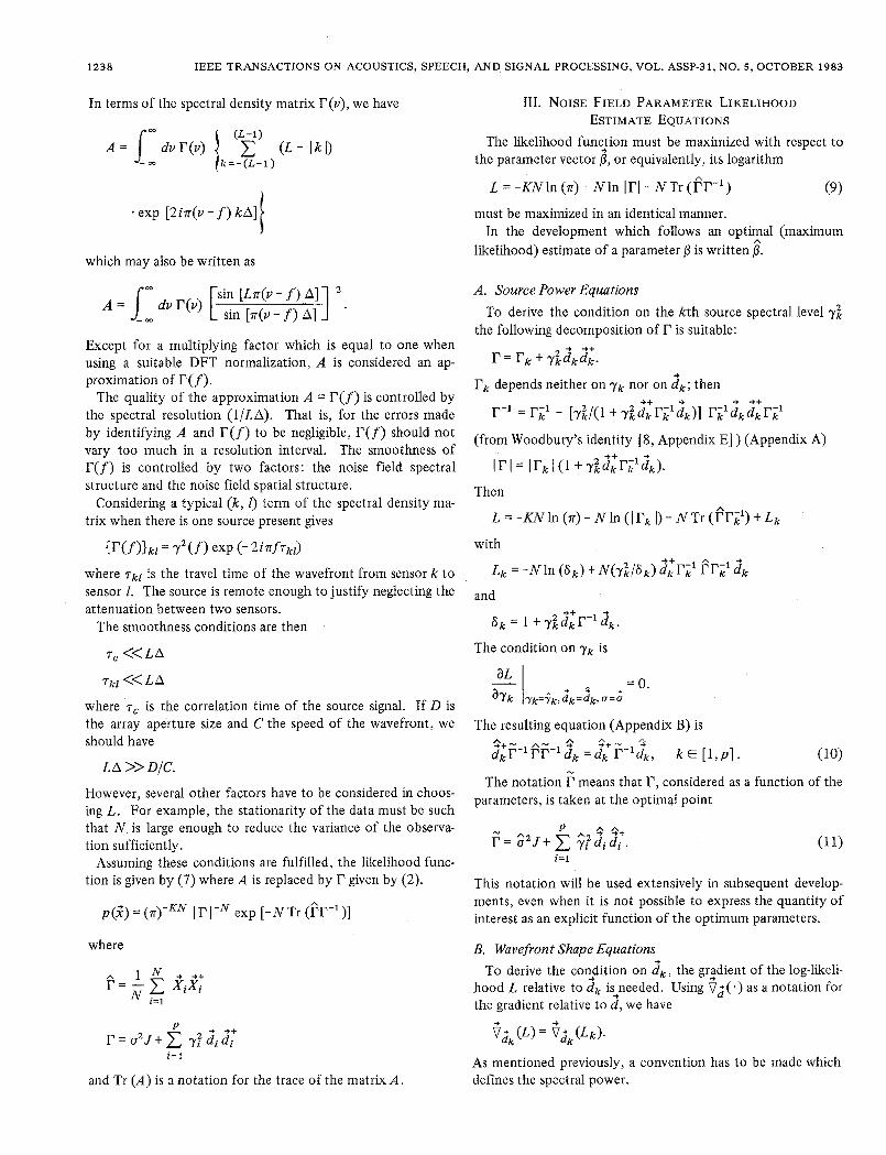
A. The Observation Space The observation vector space is spanned by the set of N out-

put samples of the system illustrated in Fig. 1. The K sensors signals ?(t) are digitized (A/D) and Fourier transformed (DFT) at frequency f into the complex N-vector of DFT coefficients

L t = C?[kA+( i - l )LA)exp( -2 in fkA)

k=l

where A is the samplingperiod and 1/LA is the spectra! resolution. An observation X will ,be iefined as the set ( X , , * * , X,) of N of the complex vectors X i .

B. Statistical Properties of the Observation The time sample vector 3(t) is assumed to be stationary,

zero-mean, and Gaussian. Thus, neglecting the digitgation errors (which introduce nonlinearities), each vector Xi will then be zero-mean and Gaussian (complex). It will be further assumed that successive samples are not correlated. The observation is then distributed according to the density

p ( 2 ) = (+KN I A exp (- 5 i;A-'?,) (7) t = l

where A is the covariance matrix + -++

A = E [ X i X i ] V i € [1 ,N] . (8)

1.4 I is the matrix A determinant and A-l its inverse.

C. Computation of the Likelihood Function Using (6) and (8), the covariance matrix A can be written

L A = exp [- 2inf(k - I> A] E[?(kA) ;'(/A)].

k , 1= 1

From (l), it is deduced

L A = exp[-2 inf (k- I>A] R[(k- I>A] .

k, 1=1

Thus, A is equal to

( L - 1 ) A = (L - I kl) exp [- 2infkAl R(kA).

k=-(L-1)

1238 IEEE TRANSACTIONS ON ACOUSTICS, SPEECH, AND SIGNAL PROCESSING, VOL. ASSP-31, NO. 5 , OCTOBER 1983

In terms of the spectral density matrix r ( v ) , we have

exp [2in(v - f ) kA] 1 which may also be written as

A =

Except for a multiplying factor which is equal to one when using a suitable DFT normalization, A is considered an approximation of I?( f ) .

The quality of the approximation A = r( f ) is controlled by the spectral resolution ( l /LA) . That is, for the errors made by identifying A and r(f) to be negligible, r( f ) should not vary too much in a resolution interval. The smoothness of r(f) is controlled by two factors: the noise field spectral structure and the noise field spatial structure.

Considering a typical ( k , I) term of the spectral density matrix when there is one source present gives

{ r ( f ) ) k l = ? ( f ) exp (-2infrkZ)

where 781 is the travel time of the wavefront from sensor k to sensor 1. The source is remote enough to justify neglecting the attenuation between two sensors.

The smoothness conditions are then

r, <<LA

rk1<< L A

where T, is the correlation time of the source signal. If D is the array aperture size and C the speed of the wavefront, we should have

L A >> DIC. However, several other factors have to be considered in choosing L . For example, the stationarity of the data must be such that N is large enough to reduce the variance of the observation sufficiently.

Assuming these conditions are fulfilled, the likelihood function is given by (7) where A is replaced by given by (2).

p(2) = ( T ) - ~ ~ I r I - N exp [ - N Tr (?T1)]

where

P r = a 2 J t C $C?i&:

i= 1

and Tr (A) is a notation for the trace of the matrix A .

111. NOISE FIELD PARAMETER LIKELIHOOD ESTIMATE EQUATIONS

The likelihood funcjion must be maximized with respect to

L = -KNln (T) - N l n Irl - N T r (i?') (9)

the parameter vector 0, or equivalently, its logarithm

must be maximized in an identical manner. In the development which follows an optimal (maximum

likelihood) estimate of a parameter /3 is written /3. n

A. Source Power Equations To derive the condition on the kth source spectral level y i

the following decomposition of I7 is suitable:

r = r& t Y i d k d k . + ++

-+ rk depends neither on Yk nor on d k ; then

r-1 = r-1 - k [ T i / ( 1 i; rL1 i k ) ] ril dk dk r,'

+ ++

(from Woodbury's identity (8, Appendix E] ) (Appendix A)

l r l = I r k l ( l t Y k k k k ) . 2 ;+r-l 2

Then

L=-KNln(n ) -Nln ( l rk I ) -NTr ( r^ rk l )+Lk

with

Lk = -N In (6,) t N ( y $ / 6 k ) 2;I-i' r^ril J k

and

6 k = 1 t Y , $ c i i r l J k .

The condition on Yk is

= 0. h k ^(k=+k,dk=dk,U=U

+ + A

The resulting equation (Appendix B) is A ++- A- 3 + - A

d k r - l r r - l ; k = d k r-'&, k E [ l , p ] . (10)

The notation r means that I?, considered as a function of the parameters, is taken at the optimal point

Y

r = G2Jt ??didi. rz rz+

i=1

This notation will be used extensively in subsequent develop- ments, even when it is not possible to express the quantity of interest as an explicit function of the optimum parameters.

B. Wavefront Shape Equations To derive the con$tion on cik, the gr2dient of the log-likeli-

hood L relative to dk is+needed. Using V;(.) as a notation for the gradient relative to d , we have

As mentioned previously, a convention has to be made which defines the spectral power.


Consider the- total power received by the array coming from a source

y2h+h.

This quantity may be measured, but to decide which is y2 and which is d d is a matter of convention. We retain

++ +

h+2 = K. (12)

Any other convention is suitable. For instance, [l 11 uses the convention y2 = 1, which leads to equivaient results. Equation (12) makes the computation easier. The optimal estimation of dk is then constrained optimization problem

( maximize Lk with respect to hk

This may be turned,into an unconstrained optimization problem using Lagrange's multiplier technique

which may be written at the optimum point as

?ik (Lk) = 2filchk

where fik is a Lagrange's multiplier.

conditions The computation of the gradient (Appendix C) leads to the

Equation (10) is easily deduced fro+m (13) (Appendix C ) . Notice that the various vectors dk are not parameterized (as

they would be if the propagation model was known). Each one of their components is free to take any value provided the constraint (12) is respected. Later on (see Section VI) it will be seen that, except for p = lJ the solution of (13) is not unique; at best, we can localize dk in a linear subspa_ce.A

Notice also that, in general, r is not equal to r. is the maximum likelihood estimate of the observation covariance matrix [see (S)] and F is a noiation [see (1 l)] . However, if p = K - 1, it will be seen that r = F, so that (13) provides no information (see Section VI).

C. Background Noise Level Equation Similarly, the maximum likelihood estimate of a requires the

solution of

The resulting equation (Appendix D) is

Tr (PF-') = K. (14)

IV. BASIC PROPERTIES OF THE NOISE FIELD PARAMETER ESTIMATES

It will now be shown, from the previous set of equations, that it is possible to derive a relationship between the noise

field maximum likelihood parameter estimate5and the eigensystem of the spectral density matrix estimate r.

This relationship is exactly the same as that between the actual noise field parameters and the eigensystem of r which have been referred to in the Introduction and are the basis of high resolution methods. That important property justifies the utilization of an estimate of the spectral density matrix instead of the spectral density matrix itself as stated by the existing asymptotical theory.

A. Property 1 The maximum likelihood estimate ? of the spectral density

matrix of the received signals I? has the same eigenvectors as the matrix F formed with the maximum likelihood estimates of the noise field parameters (1 1).

Moreover, p of these eigenvectors are in the p-dimensional linear subspace' & spanned by the maximum likelihood estimates of the p position vectors ( d l , * dp) . Th,e (K - p ) remaining eigenvectors are orthogonal to ( d l , - * , dp).

Q rz + +

Proof: First notice that & is also spanned by

Indeed, from the generalized Woodbury's identity (Appendix E), F-' can be written

The actual expression for Zii is not needed explicitly. Post- multiplying ?-' by hk gives the vector i;k:

-

Thus, Gk is a linear combination of the source position vector estimates and lies in_&. Therefore, the p vectors i$k also span &. An eigenvector of r and its related eigenvalue are such that

- . . -

From (1 1)

"2 a r- v - p yhf(di Q+r v ) di rz = x:. (1 5 )

i=1 Y

If 3 belongs to b1 the linear subspace orthogonal to b, the various scalar products in (1 5) are zero so that

"2 7- - 3 a v - h v .

Therefore, any vector in &' is an eigenvector of F, and the related eigenvalue is equal to G 2 . Since we may find (K - p ) linearly independent vectors in $I, there are (K - p ) eigenvectors of I' orthogonal to b, with the same eigenvalue G 2 . Since F is Hermitian,, its eigenvectors can be chosen orthogonal so that the remaining p eigenvectors are orthogonal to 8' and

-

1240 IEEE TRANSACTIONS ON ACOUSTICS, SPEECH, AND SIGNAL PROCESSING, VOL. ASSP-31, NO. 5, OCTOBER 1983

are then lying in 8. Let 3k be such an eigenvector. Since the vectors iCl span b, ;k can be written

'"

.., ..,

n

1=1

in terms of its-components x:. We may now write

\z=1 / 1=1

Equation (1 S),

written in terms of i i l gives -

fa, = FZ1. Using (1 7), (1 6 ) becomes

1=1

w

showing that ;k is an eigenvector Of r with the same eigenvalue. Therefore, the p eigenvectors of r lying in b are also eigenvectors of r. Because I' is Hermitian, its eigenvectors are orthogonal, thus its (K - p ) remaining eigenvectors are in bl. In other words, they are orthogonal to the maximum likelihood estimates of the source position vectors.

Moreover, we shall show that the p eigenvalues x k of i; corresponding to the eigenvectors lying in d are the largest eigenvalues of i;. ..,.., .., Taking (15) (in which 3 = & ) and left-multiplying it by i?; gives

A

A h

P ;2;;:k + r̂ ; I$+Zk12 = xkz;zk

I=1

so that (the eigenvectors are normalized)

i=l

AS ;k is lying in the dot products ( & $ ) are not all equal to zero, so that

'" A

.., hk > ;', k E [ l , p ] .

As shown above, the (K - p ) eigenvalues of i; related to the eigenvectors lying in g1 are all equal to 2 .

Finally, the eigenvalues of are split in two sets, namely the first (K - p ) all equal to ?, the eigenvectors of which are in dl, and the last p , all strictly larger than G 2 , the eigenvectors of which are in 8.

B. Property 2 The p eigenvectors of r lying in the space 8 spanned by the

p maxlmum likzlihood estimates of the sources positions vectors ( d l , . * , d p ) are related to the p largest eigenvalues of f . Thus the (K - p ) eigenvectors of r̂ related to the (K - p ) smallest eigenvalues are orthogonal to the maximum likelihood estimates of the source position vectors. The maximum likelihood estimate of the background noise spectral density G2 is given by

A

* +

which is the average of the (K - p ) smallest eigenvalues. Fi- nally, the maximum likelihood estimates of the noise field parameters are such that

i=l i=l

A 2 where Xi and wi (i E [ 1, p ] ) are the p largest eigenvalues and related eigenvectors of f . This corresponds to the asymptotical (3).

Proof: It has been shown in the precehding section that the eigenvectors of are eigenvectors of I?. It has also been shown that the p largest eigenvalues of F are r%lated to eigenvectors lying in b and that p eigenvalues of r are equal to those, but it is not clear that they are the largest.

h Let us rank the eigenvalues of r in decreasing order:

A

$1 2 x 2 X k > o .

From (18), if & is an eigenvector of i; lying in E , .-d

i;Z k - x - k u k *

Then A'" - r ; k = hk ;k

so that there exists an index e(k) such that A

he(k) = hk Y

and A '"

;e(k) = ;k*

However, all that is known is that e(k) > k and that e(1) <

Let E ( p ) be the set of in$exes e(k) , k E [ 1, p ] , so that the e(2) < . . . < e(p) . We are going to show that e(k) = k.

corresponding eigenvectors Ge(k) are in 8.

m ) = [e(l), * * * > 4P)I .

The problem is to find this set. As the maximum likelihood estimates of the noisefield pa-

rameters are such that the likelihood function or equivalently its logarithm is maximum, the set E ( p ) should be such that L is a maximum. From (9) we have

,-

L = - K N l n ( n ) - N l n ( l F l ) - N T r ( F F - ' )


and using (14), we deduce

i = - m l n ( n ) - N l n (IFI)- KN. (20)

I F I can be written in terms of the eigenvalues of e: Thus, we see that I I should be minimum.

IF1 = ( 2 ) f C - P n ^hi. i E E ( p )

It is shown in Appendix F that

~ [ p , E ( ~ ) I = x i / ( K - K - p n :i (23) L P ) i E E ( P )

such that z will be maximized by minimizing F [ p , E(p)] . are such that

The eigenvalues xi of F related to eigenvectors lying in &

"d

hj > $2.

^hi > $2 v i E E ( p ) .

h i > ' & / i ~ ( ~ - p ) v i E E ( p ) (24)

Using (19) we have

In other words, from (22) A

j @ ( p )

where e ( p ) is the largest index of E@). Thus, is the smallest eigenvalue of the set i E [l , p]}. Let E ( p ) be written

n

E ( p ) = [E(P - 117 e@>l

with

E ( p - 1) = W ) , * * * , e(P - 111 F [ p , E@)] can be written

which can be rewritten as

w h e r e \ k ( x , K - p ) = x ( l - ~ ) ~ - ~ ; x E ( O , l ] . It is shown in Appendix G .that \k is decreasing for

x > l / ( K - p + 1).

However, because

and [from (24)] A

h e ( p ) > ^hi/(K- P I ,

we have

a - ^hi<(K- p + 1 ) i E E ( p - 1 )

This results in

This implies that L is maximum only if E ( p ) is such that i e ( p )

is larger than any eigenvalue sf; j EE(p) . Indeed, if we could find 4 $ZE(p) such that ^hq > ̂ he(p) by permuting e(p) and 4, E ( p - 1 ) would not be changed. Moreover, \k would be decreased as would ,be F(p , E(p ) ) . This means that the (K - p ) eigenvectors hi; j E E ( p ) are the smallest ones, and so e ( k ) = k , k E [ l ,p] .

[ 1 , * . . , P l .

Consequently, the (K - p ) eigenvectors of ? related to the (K - p ) smallest eigenvalues are orthogonal to ( d l , * . * , d p ) .

Using (22), we obtain

rz rz

n where now ( h p + l , * , X,) are the smallest eigenvalues of r. A n

From ( F l ) we deduce

i= 1 i=l

V. DETECTION TEST FOR THE NUMBER OF SOURCES

To find the number of sources p is a multiple testing problem; p has to be chosen between 0 and (K - 1) where (K - 1) is the maximum allowed number of sources in the model. The method used is the generalized likelihood ratio test, as intro- duced in Section 11.

1242 IEEE TRANSACTIONS ON ACOUSTICS. SPEECH, AND SIGNAL PROCESSING, VOL. ASSP-3 1, NO. 5 , OCTOBER 1983

Symbolizing ;he set of unknown parameters in the p source assumption by p p , we have

iP = (0; (Yk, k E [ I , PI 1. To test a “p-sources’’ assumption against a “q-sources” assumption we use

In other words,

where f a is the false alarm probability and qp, (fa) the corresponding threshold fixed by

A

Pr MTI~, $p)/p(i~uj / 3 ~ 2 v p q ~ f u ) ~ ~ q > =fa- This method would be suitable if we are sure to be in either of these situations, but in general this is not the case.

The various quantities p ( X l p , p P ) have been computed in + r :

i(<p> = p (2 I p , FP) = (ne>-KN [F(P)] -N. (27)

the previous section. Using (9), (14), and (23) gives

F ( p ) is given by (23) where E ( p ) is now known:

To define a detection test for multiple hypothesis is possible from the theoretical point of view, when we are able to attach a cost to any decision H p (given that Hq is true) and when the a priori probabilities of the various assumptions are known. However, in practice, it is almost impossible to evaluate the cost of H p given Hq when the a priori probabilities are unknown. A suitable criterion would be a generalization of the Neyman-Pearson approach to multiple testing. However, few results are available in this field and even the concept of false alarm is not quite clear in this case. Despite the problem of choosing a reasonable criterion, the procedure always leads to a comparison of likelihood ratios (or a linear combination of likelihood ratios) to thresholds. Therefore, these are the important quantities to compute. Thus, we want to evaluate the form

[L (PYL (411 = [F(q)/F(p)l N . (29)

Finally, the detection tests have the following important properties: dependence only on the eigenvalues of the estimated spectral density matrix (whatever the criterion), and invariance with respect to the total received power for the noisefield. This latter property follows because if the signals received by the sensors are all multiplied by G, then the estimated spectral density is multiplied by G 2 , as are its eigenvalues. Thus, (29) is unchanged. These tests will only be sensitive to the distribution of the total received power between the various eigenvalues. The set of eigenvalues is a “mirror” of the power distribution between the sources and the background noise.

An interesting test which makes use of a false alarm criterion can be established. A sequence of binary (composite) tests is performed for each value of p to decide between the following two hypotheses. The first hypothesis is the most likely of the (K - p - 1) assumptions to have more than p sources.

The likelihood of this situation is

M a x p < q < ~ - l L ( 4 ) (situationgp). A

The second hypothesis is the most likely of the p assumptions to have a maximum of p sources. Its likelihood is

A

MaxqGp L(q) (situation H p ) .

The test, being the generalized likelihood ratio test, is given by

where the threshold is defined by

P r IA(p)>vp[ fa (p )1 I~ , (no source)} =f , (p ) . (30)

fa@) may depend on p or not (“false alarm” policy). ^p is the value of p such that

N p ^ > 77; If, (PI1

Np̂ + 1) < 7); [fu (PI1 .

and

Due to the monotonic form of ?(q) as a function of q (Ap- pendix G), we have

Starting sequentially from p = 0, the likelihood of having one more source than in the preceding step is tested. The decision is controlled by the probability of detecting one more source in background noise only.

This is actually a test which concerns the repartition of the smallest eigenvalues of a covariance matrix. As the test function (31) at step p depends only on the (K - p ) smallest eigenvalues, the actual hypothesis tested is that the ( K - p ) smallest eigenvalues are likely to be distributed as the eigenvalues of a “noise-only’’ situation. This, together with the way the thresholds are adjusted, is justified only if the distribution of the (K - p ) smallest eigenvalues does not depend on the p largest eigenvalues (when there are actually p sources). To a first order approximation, this seems to be justified [ 101 .

The above test can be written equivalently as

This test, known in the time series analysis literature as a “covariance matrix test for the equality of the (K - p ) smallest eigenvalues,” has been proposed in the underwater passive listening domain by Ligget [ I ] on a “heuristic” ground. We can see now in which context it can be justified.


Establishing the thresholds defined by (30) is difficult. is distributed according to the complex Wishart distribution (if N>,K - 1) and the theoretical distribution of the eigenvalues of F has been worked out [9] so that it is theoretically possible to solve the problem. Unfortunately, the expressions are quite untractable for practical use.

An asymptotical (approximate) theory has been developed in [ lo] . This approach is only valid for large N with well separated largest eigenvalues. This is not the case for low signal-to-noise ratios or close1y"spaced sources.

As has been pointed out above, the likelihood ratios are in- variant with the total power. Thus, the decision thresholds can always be determined empirically for a given false alarm probability.

VI. COMMENTS 3

Estimators for the wavefront dk and sources spectral levels ;: have not been found explicitly and we shall now show that the problem is ambiguous by nature. Fortunately (but quite naturally), this ambiguity does not affect the derivation of a detection test.

It has been shown that

i=l i=l

with

2 There w i is the eigenvector of r related to the eigenvalue hi (ith largest).

Equations (25) and (26) summarize the conditions which must be checked by the various estimators in order to fulfill the initial requirements.

It is known [ l ] , [ l l ] , [12] that (26) cannot be solved completely without a priori information about the wavefront shapes. But the problem would be of a different nature if such information were available, since it should have been used in the model to derive the optimal conditions [ 131 .

A

The solution of (26) is given by

where A is the diagonal ( p X p) matrix

and V the (K X p ) matrix of eigenvectors h

The p unknown vectors (;k) k = 1, p are p-component vectors which form an orthonormal system. The derivation of this result may be found in [14]. A better proof is given in Appendix H.

Provided the stipulated, conditions are satisfied, any choice on ik is suitable to optimize the likelihood. We say the problem is ambiguous.

An equation may ,be found relating the maximum likelihood estimates of yk and dk [14] .

which is independent of Gk (k = 1, p). However, there is an important exception to this ambiguity

situation, namely when only one source is present in the medium. In this case, the only vector Ck is reduced to a scalar which may be taken equal to one.

The optimal esti%ate of the only position vector dl is then the eigenvector of r related to the largest eigenvalue. We have been able to estimate this shape with no a priori assumptions on the wavefront shape. This may be useful in studies of propagation models.

In the peculiar case p = K - 1, (25) and (26), which summarize the problem conditions, take a very compact form. From (25)

-+

A A

a2 = hk.

From (26)

then

yielding to

F = P. VII. CONCLUSION

The general conclusion of the present study is that with a priori hypotheses made on the noise field, the optimum processing obtained by using a generalized maximum likelihood strategy leads to the utilization of the eigenvalues and eigenvectors of the spectral density matrix estimate. More specifically, two important results have been obtained.

First, a justification has been developed for the optimality of high resolution methods. Previously, only heuristic argu- ments in the asymptotical case have been proposed, stating that the eigensystem of the spectral density matrix is algebra- ically related to the noise field parameters. It has been proved that the same relationship exists between the maximum likelihood estimates of the noise field parameters and the eigensystem of the maximum likelihood estimate of the spectral density matrix.

Secondly, detection tests for the number of sources are proposed which are independent of any assumption about the wavefront shapes. They depend only on the eigenvalues of the spectral density matrix estimate. These tests are useful for detection in complex propagation conditions as in coherent multipath situations. The determination of the number of sources is compulsory for high resolution methods to be applied. A covariance matrix test suggested by Ligget [ l ] for equality of the eigenvalues of the spectral density matrix has


been derived exactly and the conditions in which it is justified have been made clear.

Numerous issues remain to be considered. The criterion which has been obtained for detection seems reasonable particularly in view of preliminary performance results [15] . However, at this stage, the criterion is still somewhat arbi- trary due to a conceptual difficulty encountered in any multiple hypothesis testing situation. Specifically, it is necessary to define practical decision costs. A feasible way to set the decision thresholds would also need further investigation. This requires the development of good quality approximations of the eigenvalue statistics. It should be kept in mind that a small loss [ 151 of detection performance over conventional methods when working on undistorted wavefronts is an unescapable price of robustness. Moreover, the value of these methods is in the high spatial resolution exhibited compared to conventional methods.

APPENDIX A A MATRIX DETERMINANT IDENTITY

It is desired to prove that

l r l = I r k I ( 1 ' Y k k k k ) . 2 ;+p-1 ;

The matrix r k is a Hermitian, positive matrix, which is therefore reducible under the Cholesky rule to

r k = cc'. Now

r = r k t y$;k;l

= c(It y$c-l;kjk+c-l+) c+ so that

Irl= ICI l z t $ G + l IC+I

= ICC+( I I t

with

;= C-';k.

The matrix I t y i ;;+ has (K - 1 ) eigenvalues equal to 1 ; the last, largest eigenvalue is (1 t y i ;+ since

(1ty;Uu ) u = ; t y $ ( u u ) u +++ + +++ -t

2 + + + + = ( I +YkU u ) u .

The determinant of any matrix is the product of its eigenvalues, so that

IIt y;;;+1= 1 + T i ; + ;

= 1 t 7; (e-' 2k )+ (c-' J k )

= l t Y k k 2 (j+c-l+c-l (jk

since

r k = cc+ ril = (c+)-l c

and

?$;;+I= 1 t Y i & r i 1 2 k .

APPENDIX B SOURCE POWER EQUATIONS

+ The maximum likelihood estimates of ( y k , u, d k ) are such

that

%I + s = 0.

'yk=$k,U=a^,dk=dk

The quantities r, r k , 8 k are functions of the noisefield parameters, In order to simplify the notation, the values of these functions - at the optimal point are simply written ?, F k , and 8 k , respectively. This general notation with the "wiggle" is used throughout the main text. Thus,

can be written, after multiplying by 8 k / 2 y k , at the optimal point as

From the expression for $k there results

so that

APPENDIX C WAVEFRONT SHAPE EQUATIONS

The maximum likelihood estimates of the noise field parameters are such that

+ The gradient of Lk relative to dk is

BIENVENU. AND KOPP: HIGH RESOLUTION ARRAY PROCESSING 1245

At the optimal point, using (Bl) for the second term yields with

. - T i - 5 3

= -2 - (NSkri ldk - N?il r r i ' d k ) = Pkdk (cl) To compute I T 1 Woodbury's identity may be applied (Ap- A - f ,$

6 k pendix E). This takes the form and using (B2) yields

A h - A

A

-2y^gFk1N(dk - m-'&)= G k z k . (c2) r-l = - - aiididi . (D2) I * + + +

I o2 i,i=1

Multiplying (C2) on the left by 2; and using (10) gives An explicit expression of aii is not needed. Now A

Gk = 0 P

so that Pr-2 = ?r-l(z/O2 - aiiciiiil?) A - 2 ' 3 i , j = 1 r r - l d k = d k . (13) fr-1 P

++ -_ u2 i,i=1 Equgion (13) implies (10) after a left multiplication of (13) - --- x aii Pr-l di& by ( d k r 1.

APPENDIX D NOISE POWER EQUATION

The maximum likelihood estimates of the noise field parameters are such that

Since

Irl=(02)>K-p(02 +hl)...(02 +AP) where hl , . . , hp do not depend on 0, then

Moreover, since

rr-l = I

and

ar - = 20Z) a0

At the optimal point, using (13), A - f f rr-' di = di

[from (D2)] . Finally,

and, from (Dl), the equation a L / h = 0 leads to

Tr (PF-l) = K . (14)

APPENDIX E WOODBURY'S IDENTITY [SI

The inversion identity is

(A t UV+)-' = A -' - A -' U(Zp t V'A-' U>-l V"A-' ,

an expression which may be easily checked for:

A = K X K matrix

U , V any K X p matrix

Zp : p X p identity matrix.

This expression is particularly useful when p = 1 (U, V are vectors) wherein

If

A t U V + = 0 2 I t , , , +

a= (zl, * * , dP) a (K X p ) matrix

y = diag (T: ) * . * , y;) a ( p X p ) diagonal matrix

with


defining U = 9 y and V =a The inverse of F can be written as

I 1 IT2 u2

(A t uv+)-' = - - - a y(u21p t e, +e,y)-' a +

Defining

Y a = - (a21p t a +a,>-, , U2

it may be written

I (a21 t a ye,+)-l = (T2 - a y a +

or, in terms of the coefficients of the matrix a

Therefore,

This expression is used in the main text. and

APPENDIX F K MATRIX IN TERMS OF ITS EIGENSYSTEM T r ( e ) = E ^xi= E ^xi+ E hi.

A

The matrix f' (1 1) can be written in term of its eigensys- i=1 i E E ( P ) i @ ( P )

tem as

i=l i=p+l

Since the eigenvectors form an orthonormal base

i=l

so

7 % + 7 % + 2 v iv i = I - E vivi i=p+l i=l

and

i=l

Therefore,

From (Fl) we get

Equation (F2) becomes

K Tr ( f ? - ' ) = (%;' - $ - 2 ) ^xi+ E ̂x i / $ 2

if=E(P) i=l

1 = p t - E hi. A

G 2 i $ E ( p )

From (14)

Tr ( ? F - ' ) = K

which combined with (F3) leads to

1 $2 =- C hi. A

K - P i e E ( p )

APPENDIX G MONOTONICITY OF THE GENERALIZED LIKELIHOOD

The function Q(x, K - p) = x ( l - x)"-" is defined on the ( ~ 1 ) domain x E [0, 13 . Its maximum value is reached when x = x.

for which

* ' ( x o ) = (1 - xo)"-"-' [ I - ( K - p t l ) x o ] =o.

x0 = (K - p t l)-l

Then with

and since ( 1 - X ~ ) ~ - P - ' > 0 , it follows that $ is decreasing for x>xo .

The maximum value of * is then

* ( X , ) = (K - P ) ( ~ - P ) / ( K - p t l ) (K-p+l)


so that

9 (x) < ( K - p ) K - p V x E [O, l [ . (K - p t 1)K-p+*

The function F ( p ) = F [ p , E ( p ) ] with E ( p ) = (1, . - , p ) in- troduced in the main text was such that

In other words

with

But *(x) < *(xo), then F ( p ) < F ( p - l), so that since the likelihood is

2 ( p ) = (ne)-KN [F(P)I - N 2

there results

2 ( p > > 2 ( q ) if p > q .

APPENDIX H PROOF OF (27) BY THE SVD THEOREM

Let us define the K rows, p columns matrix D

and the diagonal ( p X p ) matrix

y = diag ( y?) z i = l , p . A

We may then define the (K X p ) , rank p matrix

A = Dyllz

and apply the SVD (singular value decomposition) theorem to A , which says that we may write

A = UA W c (HI)

where U is a(K X K ) unitary matrix,, W is a ( p X p ) unitary matrix, and A is a(K X p ) “diagonal” matrix

(A),,=O V k f l .

Equation (26) may be written as

AA” = VAV’

where Vis a (K X p ) matrix ?5 Q v = (w1, * . * , op)

and A is a ( p X p ) diagonal matrix A A

A = diag ( X i - u ’ ) ~ = ~ , ~ .

Comparing ( H I ) to (Hz),

AA’ = UAA+U’

= VAV’

yields to

U A = VA1/’.

. So that we get finally D = VA1/2 W + Y

which can be written column by column as (32). Notice that ’ there are no conditions on W except that it be unitary. This is

because there is nothing like condition (H2) concerning the product A+A.

Previous derivation of (32) (as in [14]) may now be seen as proof of the SVD theorem.

ACKNOWLEDGMENT The authors wish to thank the reviewers for their fruitful

help in reaching the final form of this paper.

REFERENCES [ l ] W. S . Ligget, “Passive sonar: Fitting models to multiple time

series,” in Proc. NATO ASZ Signal Processing, Loughborough, England, 1972, pp. 327-345.

[2] G. Bienvenu, “Influence of the spatial coherence of the background noise on high resolution passive methods,” in Proc. ZCASSP ’79, Washington, DC, Apr. 2-4, 1979, pp. 306-309.

[3] N. L. Owsley, “An adaptive search and track array (ASTA),” NUSL Tech. Memo. 2242-166-69, July 7, 1969.

141 R. 0. Schmidt, “Multiple emitter location and signal parameters estimation,” in Proc. RADC Spectrum Estimation Workshop, Oct. 1979.

[5] G. Bienvenu and L. Kopp, “Adaptivity to background noise spatial coherence for high resolution passive methods,” in Proc. ICASSP ’79, Washington, DC, Apr. 2-4,1379, pp. 306-309.

[6] N. L. Owsley and J. F. Law, “Dominant mode power spectrum estimation,” in Proc. ZCASSP’82, Paris, France, May 3-5, 1982, pp. 775-778.

[7] H. L. Van Trees, Detection, Estimation and Modulation Theory, Part Z. New York: Wiley, 1968.

[8] A. S . Householder, The Theory of Matrices in Numerical Analy- sis. New York: Blaisdell, 1964.

[9] P. T. James, “Distributions of matrix variates and latent roots derived from normal samples,” Ann. Math. Statist., vol. 35, pp.

[ 101 -, “Test of equality of latent roots of the covariance matrix,” in Multivariate Analysis, P. R. Krishnaiah, Ed. New York: Academic, 1969, pp. 205-208.

[ 111 H. Mermoz, “Imagerie, correlation et mod&,” Ann. TiMcom- mun., vol. 31, pp. 17-36, Jan.-Feb. 1976.

[12] G. Bienvenu and L. Kopp, “Adaptive high resolution passive methods,” in Proc. EUSZPCO ’80, Lausanne, Switzerland, Sept.

[ 131 F. C . Schweppe, “Sensor-array data processing for multiple-signal sources,”ZEEE Trans. Inform. Theory, vol. IT-14, pp. 294-305, Mar. 1968.

[ 141 G . Bienvenu and L. Kopp, “Source power estimation method as- sociated with high resolution bearing estimation,” inProc. ICASSP ’81, Atlanta,GA, Mar. 30-Apr. 2, 1981, pp. 153-156.

[15] L. Kopp, G. Bienvenu, and M. Aiach, “New approach to source detection in passive listening,” in Proc. ZCASSP ’82, Paris, France, May 3-5,1982, pp. 779-782.

475-501,1964.

16-19,1980, pp. 715-721.

Georges Bienvenu (AY82-M’83) was born in Perpignan, France, in 1941. He graduated from the Ecole SupBrieure d’Electricit6, Paris, France, in 1964, and received the Ing6nieur Docteur degree from the Facult6 des Sciences d’Orsay, Orsay, France, in 1973.


A Fast Kalman Filter for images Degraded by Both Blur and Noise

Abstract-In this paper a fast Kalman filter is derived for the nearly optimal recursive restoration of images degraded in a deterministic way by blur and in a stochastic way by additive white noise. Straightfor- wardly implemented optimal restoration schemes for two-dimensional images degraded by both blur and noise create dimensionality problems which, in turn, lead to large storage and computational requirements. When the band-Toeplitz structure of the model matrices and of the distortion matrices in the matrix-vector formulations of the original image and of the noisy blurred observation are approximated by circulant matrices, these matrices can be diagonalized by means of the FFT. Consequently, a parallel set of N dynamical models suitable for the derivation of N lowarder vector Kalman filters in the transform domain is obtained. In this way, the number of computations is reduced from the order of U(N 4, to that of U(N log2 N ) for N X N images.

I I. INTRODUCTION

N the recent past, considerable attention has been devoted to the application of the recursive Kalman filter to restore

images degraded by both blur and additive noise. In the early paper of Aboutalib and Silverman [ I ] , the case of linear motion blur and additive noise is discussed. Their approach is based on modeling the one-dimensional (I-D) blurring process by a linear dynamic model, while the original image is modeled as the output of a line scanner as described by Nahi and Assefi [2] . The periodic nature of the scanning procedure results in a nonstationary output. This introduces complexities in the design of a stationary model which, in turn, necessitates additional approximations. The resulting model is basically a 1-D

Manuscript received May 25, 1982; revised March 23, 1983. The authors are with the Information Theory Group, Department of

Electrical Engineering, Delft University of Technology, P.O. Box 5031, 2600 GA Delft, The Netherlands.

model. Aboutalib, Murphy, and Silverman [3] have extended this approach to the case of general motion blur.

In this paper we want to use explicitly 2-D models for both the original image and the blur so that we take into account their two-parameter dependence. Two different approaches may be distinguished in the literature. Woods and Ingle [4] derive a Kalman filter for scalar observations based on a non- symmetric half-plane model for the original image. The image is filtered a pixel at a time. The second approach stems from Panda and Kak [ 5 ] , who derive an optimal Kalman filter for vector observations based on a DPCM-image model. Murphy and Silverman [6] have extended this approach to a vector Kalman filter based on a general semicausal image description. Both filters process the image one line at a time.

However, the optimal Kalman filter for the scalar observations of Woods and Ingle as well as the one for the vector observations of Murphy and Silverman are characterized by large computational and storage requirements. Therefore, Woods and Ingle introduce the ‘“reduced update” Kalman filter. By limiting the update procedure to the elements near the present point, the efficiency of the algorithm can be in- creased. To avoid large computational and storage requirements, Murphy and Silverman propose two suboptimal restoration schemes related to their optimal solution, namely, strip restoration and constrained optimal restoration, i.e., the gain matrix is constrained to be sparse.

Here we follow the line-by-line approach of [5] and [ 6 ] . We intend to exploit the specific matrix structures to reduce the number of computations. This is also done by Jain [7 ] for the nonblur case. Jain made use of a semicausal image model which introduces symmetric tridiagonal matrices. He proposes the sine transform to obtain a parallel set of scalar Kalman

0096-3518/83/1000-1248$01.00 0 1983 IEEE

Optimality of high resolution array processing using the eigensystem approach

Documents

Transcript of Optimality of high resolution array processing using the eigensystem approach