J. Math. Anal. Appl. 323 (2006) 441–455

www.elsevier.com/locate/jmaa

Lagrange multipliers theorem and saddle pointoptimality criteria in mathematical programming

Duong Minh Duc ∗, Nguyen Dinh Hoang, Lam Hoang Nguyen

National University of Hochiminh City, Viet Nam

Received 16 July 2005

Available online 28 November 2005

Submitted by B.S. Mordukhovich

Abstract

We prove a version of Lagrange multipliers theorem for nonsmooth functionals defined on normedspaces. Applying these results, we extend some results about saddle point optimality criteria in mathe-matical programming.© 2005 Elsevier Inc. All rights reserved.

Keywords: Lagrange multipliers theorem; Saddle point; Mathematical programming

1. Introduction

Let U be an open neighborhood of a vector x in a normed space E,g1, . . . , gN and f be realfunctions on U . We consider the following optimization problem with inequality constraints:

(PI)minf (y)

s.t. gi(y) � 0 ∀i = 1, . . . ,N.

If E is a Banach space, x is a solution of (PI), g1, . . . , gN and f are Fréchet differentiableat x and D((g1, . . . , gN))(x)(E) = RN , Ioffe and Tihomirov in [7] proved that there are a realnumber a0 and nonpositive real numbers a1, . . . , aN such that (a0, . . . , aN) �= 0 ∈ RN+1 and

a0Df (x) = a1Dg1(x) + · · · + aNDgN(x).

* Corresponding author.E-mail address: dmduc@hcmc.netnam.vn (D.M. Duc).

0022-247X/$ – see front matter © 2005 Elsevier Inc. All rights reserved.doi:10.1016/j.jmaa.2005.10.038

442 D.M. Duc et al. / J. Math. Anal. Appl. 323 (2006) 441–455

In [4], Halkin extended this result to the following optimization problem:

(PIE)

minf (y)

s.t. gi(y) � 0 ∀i = 1, . . . , n,

gn+j (y) = 0 ∀j = 1, . . . ,N − n.

Halkin also proved that a1, . . . , an are nonpositive. Furthermore, if g1, . . . , gN are not onlyFréchet differentiable but also C1 at x, that is the Fréchet derivatives of g1, . . . , gN exist on aneighborhood of x and are continuous at x, Ioffe and Tihomirov in [7, p. 73] proved that a0 intheir cited result is not equal to 0.

Using the notation of generalized gradients, Clarke, Ioffe, Michel and Penot, Mordukhovich,Rockafellar and Treiman have extended the above results for Lipschitz constraint functions in[3,5,6,10,11,17,19,20]. In [21,22], Ye considered the problem (PIE) with mixed assumptions ofGâteaux, Fréchet differentiability and Lipschitz continuity of constraint functions. In [8,9,12–16], using the extremal principle, Kruger, Mordukhovich and Wang consider the problem (PIE)

for locally Lipschitzian constraint functions on subsets in Asplund spaces.If N = 1, we reduced the Lagrange multipliers rule to a two-dimensional problem in [1] and

obtained a version of Lagrange multipliers theorem, in which we only required the smoothness ofthe restrictions of f and g on F ∩U , where F is any two-dimensional vector subspace containingx of E. This smoothness is very weak and may not imply the continuity of the functions.

In the next section of the present paper, we prove a discrete implicit mapping theorem (seeLemma 2.1) and apply it to extend the results in [1] to the case N > 1 for f and g, whoserestrictions on F ∩ U are smooth for any (N + 1)-dimensional vector subspace F containing x

of E. We note that our results can be applied to functions which are not C1-Fréchet differentiableneither Lipschitz continuous, even they are not continuous at x (see Remark 2.3). Applying theseresults, we extend some results of Bector et al. [2] in the last section.

2. Lagrange multipliers rule

Let U be a nonempty open subset of a normed space (E,‖ · ‖E), X be a linear subspace ofE, Z be a finite-dimensional linear subspace of X and J be a mapping from U into a normedspace Y . We consider Z as a normed subspace of X. Let v be a vector in X and x be in U . Denoteby Z(v) and Z(x, v) the vector subspaces of E generated by Z ∪{v} and Z ∪{x, v}, respectively.We put

Ux,Z = {y ∈ Z: x + y ∈ U},Jx,Z(y) = J (x + y) ∀y ∈ Ux,Z.

Then Ux,Z is an open subset of Z. We say

(i) J is (X,Z)-continuous at x on U if and only if for every v in X, there is a positive realnumber ηv such that Ju,Z is continuous at 0 for any u in Z(x, v) ∩ BE(x,ηv);

(ii) J is X-differentiable at x if and only if there exists a linear mapping DJ(x) from X into Y

such that

limt→0

J (x + th) − J (x)

t= DJ(x)(h) ∀h ∈ X;

D.M. Duc et al. / J. Math. Anal. Appl. 323 (2006) 441–455 443

(iii) J is (X,Z)-differentiable at x if and only if J is X-differentiable at x and for any v in X, ifthe sequence {(hm, tm)}m∈N ⊂ Z(v) × R converges to (h,0) in Z(v) × R then

limm→∞

J (x + tmhm) − J (x)

tm= DJ(x)(h).

Remark 2.1. Let J be a linear mapping from E into Rn, X be a linear subspace of E and Z bea finite-dimensional vector subspace of X. It is clear that J is (X,Z)-continuous at any x in E

and (X,Z)-differentiable at any x in E although it may not be continuous on E.

Remark 2.2. If J is (X,F )-differentiable at x then there are a positive real number εv and amapping φv from BE(0, εv) ∩ Z(v) into Y such that BE(x, εv) ⊂ U , limz→0 φv(z) = 0 and

J (x + z) = J (x) + DJ(x)(z) + ‖z‖Eφv(z) ∀z ∈ BE(0, εv) ∩ Z(v).

Indeed, it is sufficient to prove that

limz∈Z(v), z→0

J (x + z) − J (x) − DJ(x)(z)

‖z‖E

= 0.

We assume by contradiction that there exist a sequence {zm}m∈N in Z(v) and a positive realnumber ε such that 0 < ‖zm‖E < m−1 and∥∥∥∥J (x + zm) − J (x) − DJ(x)(zm)

|zm|E∥∥∥∥

Y

> ε ∀n ∈ N. (∗)

We put sm = ‖zm‖−1E zm ∈ Z(v). Because Z(v) is a finite-dimensional subspace of X, there

exists a subsequence {smk}k∈N of {sm}m∈N such that limk→∞ smk

= s in Z(v). Because J is(X,F )-differentiable at x then

limk→∞

J (x + zmk) − J (x)

‖zmk‖E

= limk→∞

J (x + ‖zmk‖Esmk

) − J (x)

‖zmk‖E

= DJ(x)(s).

Since Z(v) is finite-dimensional, Df (x) is continuous on Z(v) and

limk→∞DJ(x)

(zmk

‖zmk‖E

)= lim

k→∞DJ(x)(smk) = DJ(x)(s).

Then we have

limk→∞

J (x + zmk) − J (x) − DJ(x)(zmk

)

‖zmk‖E

= 0,

we get the contradiction with (∗) and we get the result.We have the following result:

Lemma 2.1 (Discrete Implicit Mapping Theorem). Let U be an open neighborhood of a vectorx in a normed linear space E, X be a vector subspace of E, F be a n-dimensional vectorsubspace of X and g be a mapping from U into Rn with g = (g1, . . . , gn). Assume that g is(X,F )-continuous and (X,F )-differentiable at x.

Put M = {y ∈ U : g(y) = g(x)} and ei = (δ1i , . . . , δ

ni ) for any i in {1, . . . , n}, where δ

ji is the

Kronecker number.Let v be in X and h1, . . . , hn be n vectors in F such that Dg(x)(v) = 0 and Dg(x)(hi) = ei

for any i in {1, . . . , n}.

444 D.M. Duc et al. / J. Math. Anal. Appl. 323 (2006) 441–455

Then there exist a sequence {sm = (s1m, . . . , sn

m)}m∈N converging to 0 in Rn and a sequence ofpositive real numbers {αm}m∈N converging to 0 in R such that

um ≡ αm

(s1mh1 + · · · + sn

mhn

) + αmv + x ∈ M ∀m ∈ N.

Proof. We can assume without loss of generality that x = 0 and g(x) = 0. Fix a vector v in X

such that Dg(0)(v) = 0. By Remark 2.1 about the (X,F )-continuity and (X,F )-differentiabilityof g at 0, there is a positive real number εv and a mapping φv from BF(v)(0, εv) ≡ F(v) ∩BE(0, εv) to Rn such that: BE(x, εv) ⊂ U , gy,F is continuous at 0 for every y ∈ BF(v)(0, εv),limy→0 φv(y) = 0 and

g(z) = Dg(0)(z) + ‖z‖Eφv(z) ∀z ∈ BF(v)(0, εv).

There is a real positive number r such that α(s1h1 + · · · + snhn + v) belongs to BF(v)(0, εv)

for any (α, s1, . . . , sn) ∈ (0, r) × Bn(0, r), where Bk(0,p) = {t = (t1, . . . , tk) ∈ Rk: ‖t‖Rk ≡√(t1)2 + · · · + (tk)2 < p}.We put

η(s) = s1h1 + · · · + snhn ∀s = (s1, . . . , sn

) ∈ Bn(0, r),

Gα(s) = α−1g(α(η(s) + v

)) ∀(α, s) ∈ (0, r) × Bn(0, r).

Because gy,F is continuous at 0 for every y in BF(v)(0, εv), we see that Gα is continuous onBn(0, r) for any fixed α in (0, r) and

Gα(s) = α−1g(α(s1h1 + · · · + snhn + v

)) = α−1g(α(η(s) + v

))= α−1Dg(0)

(α(η(s) + v

)) + α−1∥∥α

(η(s) + v

)∥∥Eφv

(α(η(s) + v

))= Dg(0)

(η(s)

) + ∥∥η(s) + v∥∥

Eφv

(α(η(s) + v

))= (

s1, . . . , sn) + ∥∥η(s) + v

∥∥Eφv

(α(η(s) + v

)) ∀s = (s1, . . . , sn

) ∈ Bn(0, r).

Note that there is a positive real number M such that ‖η(s) + v‖E � M for any s =(s1, . . . , sn) in Bn(0, r). Thus

limα→0

[sup

{∥∥φv

(α(η(s) + v

))∥∥E

:(s1, . . . , sn

) ∈ Bn(0, r)}] = 0

and ⟨Gα(s), s

⟩ = 〈s, s〉 + ∥∥η(s) + v∥∥

E

⟨φv

(α(η(s) + v

)), s

⟩� m−2{1 − mM

∥∥φv

(α(η(s) + v

))∥∥E

} ∀s ∈ ∂Bn

(0,m−1),

where m is an integer greater than r−1.Thus there is a real number αm in (0,m−1) such that⟨

Gαm(s), s⟩> 0 ∀s ∈ ∂Bn

(0,m−1).

By Lemma 4.1 in [18, p. 14], we have a solution sm in Bn(0,m−1) to the equation Gαm(s) = 0for any integer m greater than r−1, which yields the lemma. �Remark 2.3. If E is a Banach space, U is an open subset of E, g is Fréchet differentiable onU and Dg is continuous at x, then by the Ljusternik theorem (see [7, p. 41]), M is a manifoldand the tangent space T Mx = Dg(x)−1({0}). Moreover, M is a C1-manifold if g is C1-Fréchet

D.M. Duc et al. / J. Math. Anal. Appl. 323 (2006) 441–455 445

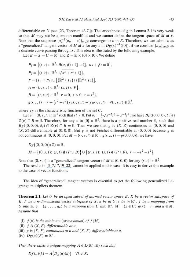
differentiable on U (see [23, Theorem 43.C]). The smoothness of g in Lemma 2.1 is very weakso that M may not be a smooth manifold and we cannot define the tangent space of M at x.Note that the sequence {α−1

m (um − x)}m∈N converges to v in E. Therefore, we can admit v asa “generalized” tangent vector of M at x for any v in Dg(x)−1({0}), if we consider {um}m∈N asa discrete curve passing through x. This idea is illustrated by the following example.

Let E = X = U = R3 and Z = R × {0} × {0}. We define

P1 = {(s, t) ∈ R2: ∃(α,β) ∈ Q × Q, αs + βt = 0

},

P2 = {(s, t) ∈ R2:

√s2 + t2 ∈ Q

},

P = [P1 ∩ P2] ∪ [(R2 \ P1

) ∩ (R2 \ P2

)],

A = {(r, s, t) ∈ R3: (s, t) ∈ P

},

B = {(r, s, t) ∈ R3: r = 0, s > 0, t = s2},

g(r, s, t) = r + (s2 + t2)χA(r, s, t) + χB(r, s, t) ∀(r, s, t) ∈ R3,

where χC is the characteristic function of the set C.Let v = (0, s, t) in R3 such that st �= 0. Put δv = 1

2

√s−2t2 + s−4t4, we have BE((0,0,0), δv)∩

Z(v) ∩ B = ∅. Therefore, for any v in {0} × R2, there is a positive real number δv such thatBE((0,0,0), δv) ∩ Z(v) ∩ B = ∅. Thus we see that g is (X,Z)-continuous at (0,0,0) and(X,Z)-differentiable at (0,0,0). But g is not Fréchet differentiable at (0,0,0) because g isnot continuous at (0,0,0). Put M = {(r, s, t) ∈ R3: g(r, s, t) = g(0,0,0)}, we have

Dg((0,0,0)

)(Z) = R,

M = {(0, s, t): (s, t) /∈ (P ∪ B)

} ∪ {(r, s, t): (s, t) ∈ (P \ B), r = −s2 − t2}.

Note that (0, s, t) is a “generalized” tangent vector of M at (0,0,0) for any (s, t) in R2.The results in [3–7,17,19–22] cannot be applied to this case. It is easy to derive this example

to the case of vector functions.

The idea of “generalized” tangent vectors is essential to get the following generalized La-grange multipliers theorem.

Theorem 2.1. Let U be an open subset of normed vector space E, X be a vector subspace ofE, F be a n-dimensional vector subspace of X, u be in U , r be in Rn, f be a mapping fromU into R, g = (g1, . . . , gn) be a mapping from U into Rn, M = {x ∈ U : g(x) = r} and u ∈ M .Assume that

(i) f (u) is the minimum (or maximum) of f (M),(ii) f is (X,F )-differentiable at u,

(iii) g is (X,F )-continuous at u and (X,F )-differentiable at u,(iv) Dg(u)(F ) = Rn.

Then there exists a unique mapping Λ ∈ L(Rn,R) such that

Df (u)(k) = Λ(Dg(u)(k)

) ∀k ∈ X.

446 D.M. Duc et al. / J. Math. Anal. Appl. 323 (2006) 441–455

Proof. Assume f (u) is the minimum of f (M). Choose n vectors h1, . . . , hn in F such thatDg(u)(hi) = ei ≡ (δ1

i , . . . , δni ) for any i in {1, . . . , n}. We define a real linear mapping Λ on Rn

as follows:

Λ(ei) = Df (u)(hi) ∀i = 1, . . . , n.

Now fix a vector k in X. Put

v = k −n∑

i=1

Dgi(u)(k)hi ∈ X.

Then Dg(u)(v) = 0. By Lemma 2.1, there are a sequence {αm}m∈N of positive real numbersand a sequence {sm = (s1

m, . . . , snm)}m∈N in Rn such that {αm}m∈N and {sm}m∈N converge to 0 in

R and Rn respectively, um ∈ U , and g(um) = g(u), where

um = u + αm

(s1mh1 + · · · + sn

mhn

) + αmv ∀m ∈ N,

or um ∈ M for every m ∈ N.Since f (u) is the minimum of f (M) and f is (X,F )-differentiable at u, we have

Df (u)(k) − Λ(Dg(u)(k)

)= Df (u)(k) − Λ

(n∑

i=1

Dgi(u)(k)ei

)

= Df (u)(k) −n∑

i=1

Di(u)(k)Λ(ei) = Df (u)(k) −n∑

i=1

Dgi(u)(k)Df (u)(hi)

= Df (u)(k) − Df (u)

(n∑

i=1

Dgi(u)(k)hi

)= Df (u)

(k −

n∑i=1

Dgi(u)(k)hi

)

= Df (u)(v) = limm→∞

[f (u + αm(s1mh1 + · · · + sn

mhn + v)) − f (u)]αm

� 0.

Therefore, Df (u)(k) � Λ(Dg(u)(k)) for any k in X. Replacing k in the above inequalityby −k, we get the theorem.

Since Dg(u)(F ) = Rn, we can get the uniqueness of Λ.The proof for the case f (u) = maxf (M) is similar and omitted. �

Remark 2.4. If E is a Banach space, g is Fréchet differentiable on U and Dg is continuous at u,then Theorem 2.1 has been proved in [7, p. 73]. Here we only need the differentiability of f andg at u. If n = 1, Theorem 2.1 has been proved in [1].

Theorem 2.2. Let U be an open subset of normed vector space E, X be a vector subspace of E,F be a (n + m)-dimensional vector subspace of X, u be in U , f be a mapping from U into R,g = (g1, . . . , gn+m) be a mapping from U into Rn+m and

M = {x ∈ U : gi(x) � 0, gn+j (x) = 0 ∀i ∈ {1, . . . , n}, j ∈ {1, . . . ,m}}.

Assume that

(i) u ∈ M and f (u) is the minimum of f (M),

D.M. Duc et al. / J. Math. Anal. Appl. 323 (2006) 441–455 447

(ii) f is (X,F )-differentiable at u,(iii) g is (X,F )-continuous at u and (X,F )-differentiable at u,(iv) Dg(u)(F ) = Rn+m.

Then g(u) = 0 and there exists a unique (a1, . . . , an+m) in Rn+m such that a1, . . . , an are nega-tive and

Df (u)(k) =n+m∑i=1

aiDgi(u)(k) ∀k ∈ X.

Proof. We prove the theorem by the following steps.

Step 1. Put α = (α1, . . . , αn+m) = g(u) and S = {x ∈ U : g(x) = α} we see that S ⊂ M . Sincef (u) = minf (S), by Theorem 2.1, there exists a unique (a1, . . . , an+m) in Rn+m such that

Df (u)(k) =n+m∑i=1

aiDgi(u)(k) ∀k ∈ X.

Step 2. We prove that ai < 0 for every i ∈ {1, . . . , n}. First, we prove that a1 < 0. SinceDg(u)(F ) = Rn+m, there is k in F such that Dg1(u)(k) = −1 and Dg2(u)(k) = · · · =Dgn(u)(k) = −ε < 0 and Dgn+j (u)(k) = 0 for any j in {1, . . . ,m}.

Let {hi}i=1,...,n+m be in F such that Dg(u)(hi) = (δ1i , . . . , δ

n+mi ) for any i ∈ {1, . . . , n + m},

we have

D(gn+1, . . . , gn+m)(u)(hi) = (δn+1i , . . . , δn+m

i

) ∀i ∈ {n + 1, . . . , n + m}.By Lemma 2.1, there are a sequence {sl = (sn+1

l , . . . , sn+ml )}l∈N converging to 0 in Rm and a

sequence of positive real numbers {αl}l∈N converging to 0 in R such that

ul ≡ αl

(sn+1l hn+1 + · · · + sn+m

l hn+m

) + αlk + u,

(gn+1, . . . , gn+m)(ul) = (gn+1, . . . , gn+m)(u) = 0 ∀l ∈ N.

Note that

liml→∞

gi(ul) − gi(u)

αl

= liml→∞

gi(αl(sn+1l hn+1 + · · · + sn+m

l hn+m) + αlk + u) − gi(u)

αl

= Dgi(u)(k) < 0 ∀i ∈ {1, . . . , n}.Thus there exists l0 ∈ N such that

gi(ul) < gi(u) ∀i ∈ {1, . . . , n}, ∀l � l0,

which implies that ul is in M for any l � l0 and

−a1 − ε

n∑i=2

ai = Df (u)(k) = liml→∞

f (ul) − f (u)

αl

� 0 ∀ε > 0.

Let ε tend to 0, we have −a1 � 0 or a1 � 0. Since Dg(u)(F ) = Rn+m, we have a1 < 0.Similarly, we have

ai < 0 ∀i = 1, . . . , n.

448 D.M. Duc et al. / J. Math. Anal. Appl. 323 (2006) 441–455

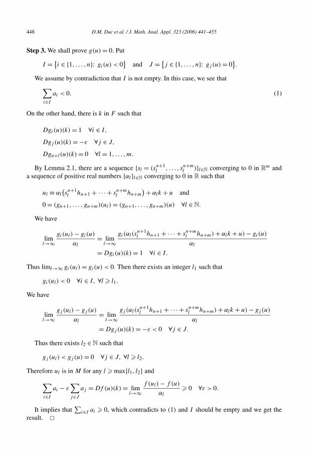
Step 3. We shall prove g(u) = 0. Put

I = {i ∈ {1, . . . , n}: gi(u) < 0

}and J = {

j ∈ {1, . . . , n}: gj (u) = 0}.

We assume by contradiction that I is not empty. In this case, we see that∑i∈I

ai < 0. (1)

On the other hand, there is k in F such that

Dgi(u)(k) = 1 ∀i ∈ I,

Dgj (u)(k) = −ε ∀j ∈ J,

Dgn+l(u)(k) = 0 ∀l = 1, . . . ,m.

By Lemma 2.1, there are a sequence {sl = (sn+1l , . . . , sn+m

l )}l∈N converging to 0 in Rm anda sequence of positive real numbers {αl}l∈N converging to 0 in R such that

ul ≡ αl

(sn+1l hn+1 + · · · + sn+m

l hn+m

) + αlk + u and

0 = (gn+1, . . . , gn+m)(ul) = (gn+1, . . . , gn+m)(u) ∀l ∈ N.

We have

liml→∞

gi(ul) − gi(u)

αl

= liml→∞

gi(αl(sn+1l hn+1 + · · · + sn+m

l hn+m) + αlk + u) − gi(u)

αl

= Dgi(u)(k) = 1 ∀i ∈ I.

Thus liml→∞ gi(ul) = gi(u) < 0. Then there exists an integer l1 such that

gi(ul) < 0 ∀i ∈ I, ∀l � l1.

We have

liml→∞

gj (ul) − gj (u)

αl

= liml→∞

gj (αl(sn+1l hn+1 + · · · + sn+m

l hn+m) + αlk + u) − gj (u)

αl

= Dgj (u)(k) = −ε < 0 ∀j ∈ J.

Thus there exists l2 ∈ N such that

gj (ul) < gj (u) = 0 ∀j ∈ J, ∀l � l2.

Therefore ul is in M for any l � max{l1, l2} and

∑i∈I

ai − ε∑j∈J

aj = Df (u)(k) = liml→∞

f (ul) − f (u)

αl

� 0 ∀ε > 0.

It implies that∑

i∈I ai � 0, which contradicts to (1) and I should be empty and we get theresult. �

D.M. Duc et al. / J. Math. Anal. Appl. 323 (2006) 441–455 449

3. Applications in programming problems

Let X ≡ Rn denote the n-dimensional Euclidean space and let Rn+ be its nonnegative or-thant. Let f,h1, . . . , hm be real functions on an open subset S of Rn. We consider the followingnonlinear programming problem

(P )minf (x)

subject to hj (x) � 0 ∀j ∈ {1,2, . . . ,m}.Put J = {1, . . . , r} and K = {r + 1, . . . ,m}, hJ (x) = (h1(x), . . . , hr (x)) and hK(x) =

(hr+1(x), . . . , hm(x)) for any x in S. Let h(x) denote the column vector (h1(x), h2(x), . . . ,

hm(x))T and be partitioned as h(x) = (hJ (x),hK(x))T . We denote

Sh = {x ∈ S: hj (x) � 0, j ∈ {1, . . . ,m}},

SK = {x ∈ S: hk(x) � 0, k ∈ K

}.

Let a = (a1, . . . , aN) ∈ RN with N ∈ N. We say a � 0 (or � 0) if and only if ai � 0 (or � 0)for every i ∈ {1, . . . ,N}.

Definition 3.1. Let S be an open subset of Rn, u be in S, g be a real function on S and Gâteauxdifferentiable at u, and η is a function from S × S to Rn. We say

(i) the function g is said to be invex at u with respect to the function η, if for every x ∈ S, wehave

g(x) − g(u) � η(x,u)T ∇g(u);(ii) the function g is said to be pseudo-invex at u with respect to the function η, if for every

x ∈ S, we have

η(x,u)T ∇g(u) � 0 ⇒ g(x) � g(u);(iii) the function g is said to be quasi-invex at u with respect to the function η, if for every x ∈ S,

we have

g(x) � g(u) ⇒ η(x,u)T ∇g(u) � 0.

Applying results in the first section, we study the following programming problems.

Problem 1: Nonlinear programming problem

Let f , g, h1, . . . , hm be real functions on an open subset S of Rn. Let J , K , hJ and hK be asin the beginning of this section.

Put L(x,λJ ) = f (x) + (λJ )T hJ (x) for any (x,λJ ) in SK × R|J |+ . The map L is called the

incomplete Lagrange function of the problem (P ).

Definition 3.2. A point (x, λJ ) ∈ SK × R|J |+ is called a saddle point of the incomplete Lagrange

function L if

L(x, λJ ) � L(x, λJ ) � L(x, λJ ) ∀(x,λJ ) ∈ SK × R|J |+ .

450 D.M. Duc et al. / J. Math. Anal. Appl. 323 (2006) 441–455

Theorem 3.1. Let S be an open subset of X ≡ Rn, f and h1, . . . , hm be real functions on S andGâteaux differentiable at x with x ∈ S. F be a m-dimensional vector subspace of X and x beoptimal for (P ). Assume that

(i) L(·, λJ ) is pseudo invex and (λK)T hK(·) is quasi invex at x with respect to a function η forany (λJ ,λK) in Rm+;

(ii) f is (X,F )- differentiable at x;(iii) h is (X,F )-differentiable at x and (X,F )-continuous at x;(iv) Dh(x)(F ) = Rm.

Then there exists λJ ∈ R|J |+ such that (x, λJ ) is a saddle point of the incomplete Lagrange func-

tion L.

Proof. Applying Theorem 2.2 in case E = X = Rn, U = S for f and {hj }j=1,m, there exists

λ = (λJ , λK) ∈ Rm, λJ ∈ R|J |+ , λK ∈ R

|K|+ , such that

∇[f (x) + (λJ )T hJ (x) + (λK)T hK(x)

] = 0,

(λJ )T hJ (x) = 0, (λK)T hK(x) = 0,

λ = (λJ , λK) � 0.

Now arguing as in the proof of Theorem 2.1 in [2], we get the theorem. �We consider the following propositions.

(A1) x be optimal for (P ).(A2) There are positive real numbers λ1, . . . , λm such that hi(x) = 0 for any i in {1, . . . ,m} and

Df (x) + λ1Dh1(x) + · · · + λmDhm(x) = 0.

We have the following result.

Theorem 3.2. Let S be an open subset of X ≡ Rn, f and h1, . . . , hm be real functions on S. Letx be in S. Then

(i) if f , h1, . . . , hm satisfy the conditions (ii), (iii) and (iv) of Theorem 3.1, then (A1) implies(A2);

(ii) if f (·)+ ∑mi=1 λihi(·) is Gâteaux differentiable at x and invex with respect to the function η

at x then (A2) implies (A1).

Proof. Applying Theorem 2.2 in case E = X = Rn, U = S for f and {hj }j=1,m, we get (i).Consider (ii). By the invexity property of f (·) + ∑m

i=1 λihi(·) with respect to the function η

at x, we have

f (x) +m∑

i=1

λihi(x) −[f (x) +

m∑i=1

λihi(x)

]

� η(x, x)T ∇[f +

m∑λihi

](x) = 0 ∀x ∈ Sh.

i=1

D.M. Duc et al. / J. Math. Anal. Appl. 323 (2006) 441–455 451

It follows that

f (x) � f (x) +m∑

i=1

λihi(x) � f (x) +m∑

i=1

λihi(x) = f (x) ∀x ∈ Sh,

and we get (ii). �Problem 2: Fractional programming problem

Let f , g,h1, . . . , hm be real functions on an open subset S of Rn. Let J , K , hJ and hK be asin the beginning of this section. Put

Sh = {x ∈ S: hj (x) � 0, j ∈ {1, . . . ,m}},

SK = {x ∈ S: hk(x) � 0, k ∈ K

}.

Assume that g(x) �= 0 for any x in S and g(x) > 0 for any x in SK . We now consider thefractional programming problem

(FP)min

f (x)

g(x)

subject to hj (x) � 0 ∀j ∈ {1,2, . . . ,m}.We note that if x is optimal for the problem (FP) then x is also optimal for the following

problem

(FP1)

minf (x)

g(x)

subject tohj (x)

g(x)� 0 ∀j ∈ J and hk(x) � 0 ∀k ∈ K.

This form of (FP1) suggests the choice of the incomplete Lagrange function LF :SK ×R

|J |+ → R as follows:

LF (x,λJ ) = f (x) + (λJ )T hJ (x)

g(x).

Definition 3.3. A point (x, λJ ) ∈ SK × R|J |+ is called a saddle point of the incomplete Lagrange

function LF if

LF (x, λJ ) � LF (x, λJ ) � LF (x, λJ ) ∀(x,λJ ) ∈ SK × R|J |+ .

Theorem 3.3. Let S be an open subset of X ≡ Rn, f and h1, . . . , hm be real functions on S andGâteaux differentiable at x with x ∈ S. F be a m-dimensional vector subspace of X and x beoptimal for (FP). Assume that

(i) LF (·, λJ ) is pseudo invex and (λK)T hK(·) is quasi invex at x with respect to a function η

for any (λJ ,λK) in Rm+;

(ii) fg

is (X,F )-differentiable at x;

(iii) h1g

, . . . , hr

g, hr+1, . . . , hm are (X,F )-differentiable at x and (X,F )-continuous at x;

(iv) D((h1 , . . . , hr , hr+1, . . . , hm))(x)(F ) = Rm.

g g

452 D.M. Duc et al. / J. Math. Anal. Appl. 323 (2006) 441–455

Then there exists λJ ∈ R|J |+ such that (x, λJ ) is a saddle point of the incomplete Lagrange func-

tion LF .

Proof. Since x is optimal for (FP) (and hence for (FP1)), applying Theorem 2.2 in case E =X = Rn, U = S for f

gand h1

g, . . . , hr

g, hr+1, . . . , hm, we can find λ = (λJ , λK) in R

|J |+ × R

|K|+ ,

such that

∇[f (x)

g(x)+ (λJ )T

hJ (x)

g(x)+ (λK)T hK(x)

]= 0,

(λJ )T hJ (x) = 0 and (λK)T hK(x) = 0.

Fix x in SK , we have (λK)T hK(x) � 0 = (λK)T hK(x). By the quasi-invexity of (λK)T hK(·)with respect to the function η at x, we obtain

η(x, x)T ∇[(λK)T hK(x)

]� 0.

Thus

η(x, x)T ∇[f (x)

g(x)+ (λJ )T

hJ (x)

g(x)

]� 0.

By the pseudo-invexity of f (·)+(λJ )T hJ (·)g(·) with respect to the function η at x, we see that

f (x)

g(x)+ (λJ )T

hJ (x)

g(x)� f (x)

g(x)+ (λJ )T

hJ (x)

g(x).

And we get

LF (x, λJ ) � LF (x, λJ ).

If λJ is in R|J |+ , we have

LF (x, λJ ) = f (x)

g(x)+ (λJ )T

hJ (x)

g(x)= f (x)

g(x)� f (x)

g(x)+ (λJ )T

hJ (x)

g(x)= LF (x, λJ ).

Thus we get the theorem. �Problem 3: Generalized fractional programming problem

Let f1, . . . , fp, g1, . . . , gp,h1, . . . , hm be real functions on an open subset S of Rn. Put

Sh = {x ∈ S: hj (x) � 0, j ∈ {1, . . . ,m}},

SK = {x ∈ S: hk(x) � 0, k ∈ K

}.

Assume that g1(x), . . . , gp(x) �= 0 for any x in S and g1(x), . . . , gp(x) are positive for everyx in Sh. We consider the generalized fractional programming problem

(GFP)minx∈S

max1�i�p

fi(x)

gi(x)

subject to hj (x) � 0 ∀j ∈ {1,2, . . . ,m}.Put Y = {y ∈ R

p+,

∑p

i=1 yi = 1}. The incomplete Lagrange function LG :SK ×Y × R|J |+ → R

for the problem (GFP) can be chosen as

LG(x, y,λJ ) = yT f (x) + (λJ )T hJ (x)

yT g(x).

D.M. Duc et al. / J. Math. Anal. Appl. 323 (2006) 441–455 453

Definition 3.4. A point (x, y, λJ ) ∈ SK × Y × R|J |+ is called a saddle point of the incomplete

Lagrange function LG if

LG(x, y,λJ ) � LG(x, y, λJ ) � LG(x, y, λJ ) ∀(x, y,λJ ) ∈ SK × Y × R|J |+ .

We consider the problem

(EGFP)v

minq

subject to fi(x) − vgi(x) � q and

hj (x) � 0 ∀(i, j) ∈ {1, . . . , p} × {1, . . . ,m}.We have the following lemma (see [2, Lemma 2.3, p. 9]).

Lemma 3.1. The point x∗ is (GFP) optimal with corresponding optimal value of the (GFP)

objective equal to v∗ if and only if (x∗, q∗) is (EGFP)v∗ optimal with corresponding optimalvalue of the (EGFP)v∗ objective equal to 0, i.e., q∗ = 0.

Now we define

Hv∗(x, q) = q ∀(x, q) ∈ S × R,

Gv∗1i (x, q) = fi(x) − v∗gi(x) − q ∀(x, q, i) ∈ S × R × {1, . . . , p},

Gv∗2j (x, q) = hj (x) ∀(x, q, j) ∈ S × R × {1, . . . ,m}.

Theorem 3.4. Let S be an open subset of X ≡ Rn, f1, . . . , fp, g1, . . . , gp,h1, . . . , hm be realfunctions on S and Gâteaux differentiable at x with x ∈ S. F be a (p + m)-dimensional vectorsubspace of X × R ≡ Rn × R and x be optimal for (GFP) with corresponding optimal value ofthe (GFP) objective equal to v∗. Assume that

(i) LG(·, y, λJ ) is pseudo invex and (λK)T hK(·) is quasi invex at x with respect to a functionη for any (y,λJ ,λK) in Y × Rm+;

(ii) Gv∗11, . . . ,G

v∗1p , Gv∗

21, . . . ,Gv∗2m are (Rn × R,F )-differentiable at (x,0) and (Rn × R,F )-

continuous at (x,0);(iii) D((Gv∗

11, . . . ,Gv∗1p , Gv∗

21, . . . ,Gv∗2m))(x,0)(F ) = Rp+m.

Then there exists (y, λJ ) ∈ Y × R|J |+ such that (x, y, λJ ) is a saddle point of the incomplete

Lagrange function LG.

Proof. Because x is an optimal value of (GFP) with corresponding optimal value of the (GFP)

objective equal to v∗, by Lemma 3.1, (x∗, q∗) is (EGFP)v∗ optimal with corresponding optimalvalue of the (EGFP)v∗ objective equal to 0. Then the problem

(L)minHv∗

(x, q)

subject to Gv∗1i (x, q) � 0 and Gv∗

2j (x, q) � 0 ∀(i, j) ∈ {1, . . . , p} × {1, . . . ,m}has an optimal solution (x∗, q∗) with q∗ = 0.

454 D.M. Duc et al. / J. Math. Anal. Appl. 323 (2006) 441–455

Applying Theorem 2.2 in case E = X = Rn ×R, U = S ×R for Hv∗and Gv∗

11, . . . ,Gv∗1p,Gv∗

21,

. . . ,Gv∗2m, there exists (y, λJ , λK) ∈ R

p+ × R

|J |+ × R

|K|+ such that

DHv∗(x,0)(k, l) +

p∑i=1

yiDGv∗1i (x,0)(k, l) +

m∑j=1

λjDGv∗2j (x,0)(k, l) = 0, (∗)

for every (k, l) ∈ Rn × R and

yi

[fi(x) − v∗gi(x)

] = 0 ∀i ∈ {1, . . . , p},(λJ )T hJ (x) = 0, (λK)T hK(x) = 0, λ = (λJ , λK) � 0, y � 0.

If l in (∗) is equal to 0, we have

∇[yT f (x) − v∗yT g(x) + (λJ )T hJ (x) + (λK)T hK(x)

] = 0.

If k in (∗) is equal to 0, we have∑p

i=1 yi = 1 or y ∈ Y .Now arguing as in the proof of Theorem 2.5 in [2], we get the theorem. �We consider the following propositions:

(A3) x be optimal for (GFP) with corresponding optimal value of the (GFP) objective equalto v∗.

(A4) x has the following properties:

∇[yT f (x) − v∗yT g(x) + (λJ )T hJ (x) + (λK)T hK(x)

] = 0,

yi

[fi(x) − v∗gi(x)

] = 0 ∀i ∈ {1, . . . , p},(λJ )T hJ (x) = 0, (λK)T hK(x) = 0, λ = (λJ , λK) � 0, y � 0,

p∑i=1

yi = 1.

Theorem 3.5. Let S be an open subset of X ≡ Rn, f1, . . . , fp, g1, . . . , gp,h1, . . . , hm be realfunctions on S. Let x be in S.

(i) If the conditions (ii), (iii) of Theorem 3.4 are fulfilled then (A3) implies (A4).(ii) If yT f (·) − v∗yT g(·) + (λJ )T hJ (·) + (λK)T hK(·) is Gâteaux differentiable at x and invex

with respect to the function η at x then (A4) implies (A3).

Proof. Applying Theorem 2.2 in case E = X = Rn ×R, U = S ×R for Hv∗and Gv∗

11, . . . ,Gv∗1p,

Gv∗21, . . . ,G

v∗2m (we define in p. 453) and with the same proof of Theorem 3.4, we get (i).

Consider (ii). Since the map yT f (·) − v∗yT g(·) + (λJ )T hJ (·) + (λK)T hK(·) is invex withrespect to the function η at x, for every x ∈ Sh, we have

yT f (x) − v∗yT g(x) + (λJ )T hJ (x) + (λK)T hK(x)

− [yT f (x) − v∗yT g(x) + (λJ )T hJ (x) + (λK)T hK(x)

]� η(x, x)T ∇[

yT f (x) − v∗yT g(x) + (λJ )T hJ (x) + (λK)T hK(x)] = 0.

D.M. Duc et al. / J. Math. Anal. Appl. 323 (2006) 441–455 455

Thus

yT f (x) − v∗yT g(x) � yT f (x) − v∗yT g(x) + (λJ )T hJ (x) + (λK)T hK(x) � 0.

It implies that Maxi=1,pfi (x)gi (x)

� v∗, for every x ∈ Sh and we get (ii). �Acknowledgments

The authors thank the referees for very helpful comments.

References

[1] L.H. An, P.X. Du, D.M. Duc, P.V. Tuoc, Lagrange multipliers for functions derivable along directions in a linearsubspace, Proc. Amer. Math. Soc. 133 (2005) 595–604.

[2] C.R. Bector, S. Chandra, A. Abha, On incomplete Lagrange function and saddle point optimality criteria in mathe-matical programming, J. Math. Anal. Appl. 251 (2000) 2–12.

[3] F.H. Clarke, Optimization and Nonsmooth Analysis, Wiley–Interscience, New York, 1983.[4] H. Halkin, Implicit functions and optimization problems without continuous differentiability of the data, SIAM J.

Control 12 (1974) 229–236.[5] A.D. Ioffe, Necessary conditions in nonsmooth optimization, Math. Oper. Res. 9 (1984) 159–189.[6] A.D. Ioffe, A Lagrange multiplier rule with small convex-valued subdifferentials for nonsmooth problems of math-

ematical programming involving equality and nonfunctional constraints, Math. Programming 58 (1993) 137–145.[7] A.D. Ioffe, V.M. Tihomirov, Theory of Extremal Problems, Nauka, Moscow, 1974 (in Russian).[8] A.Y. Kruger, Generalized differentials of nonsmooth functions and necessary conditions for an extremum, Siberian

Math. J. 26 (1985) 370–379.[9] A.Y. Kruger, B.S. Mordukhovich, Extremal points and the Euler equation in nonsmooth optimization, Dokl. Akad.

Nauk BSSR 24 (1980) 684–687.[10] P. Michel, J.-P. Penot, Calcul sous-différentiel pour des fonctions lipschitziennes et non lipschitziennes, C. R. Acad.

Sci. Paris Sér. I Math. 12 (1984) 269–272.[11] P. Michel, J.-P. Penot, A generalized derivative for calm and stable functions, Differential Integral Equations 5

(1992) 433–454.[12] B.S. Mordukhovich, Metric approximations and necessary optimality conditions for general classes of nonsmooth

extremal problems, Soviet Math. Dokl. 22 (1980) 526–530.[13] B.S. Mordukhovich, On necessary conditions for an extremum in nonsmooth optimization, Soviet Math. Dokl. 32

(1985) 215–220.[14] B.S. Mordukhovich, An abstract extremal principle with applications to welfare economics, J. Math. Anal.

Appl. 251 (2000) 187–216.[15] B.S. Mordukhovich, The extremal principle and its applications to optimization and economics, in: A. Rubinov,

B. Glover (Eds.), Optimization and Related Topics, in: Appl. Optim., vol. 47, Kluwer Academic, Dordrecht, 2001,pp. 343–369.

[16] B.S. Mordukhovich, B. Wang, Necessary suboptimality and optimality conditions via variational principles, SIAMJ. Control Optim. 41 (2002) 623–640.

[17] R.T. Rockafellar, Convex Analysis, Princeton Univ. Press, Princeton, NJ, 1970.[18] V. Skrypnik, Methods for analysis of nonlinear elliptic boundary value problems, Amer. Math. Soc., Providence,

RI, 1994.[19] J.S. Treiman, Shrinking generalized gradients, Nonlinear Anal. 12 (1988) 1429–1450.[20] J.S. Treiman, Lagrange multipliers for nonconvex generalized gradients with equality, inequality, and set constraints,

SIAM J. Control Optim. 37 (1999) 1313–1329.[21] J.J. Ye, Multiplier rules under mixed assumptions of differentiability and Lipschitz continuity, SIAM J. Control

Optim. 39 (2001) 1441–1460.[22] J.J. Ye, Nondifferentiable multiplier rules for optimization and bilevel optimization problems, SIAM J. Optim. 15 (1)

(2004) 252–274.[23] E. Zeidler, Nonlinear Functional Analysis and Its Applications, III: Variational Methods and Optimization, Springer,

Berlin, 1985.