R. Huang et al. (Eds.): ADMA 2009, LNAI 5678, pp. 595–602, 2009. © Springer-Verlag Berlin Heidelberg 2009

Application of the Cross-Entropy Method to Dual Lagrange Support Vector Machine

Budi Santosa

Department of Industrial Engineering, Institut Teknologi Sepuluh Nopember Surabaya 60111 Kampus ITS Surabaya, Indonesia

budi_s@ie.its.ac.id

Abstract. In this paper, cross entropy method is used for solving dual Lagrange support vector machine (SVM). Cross entropy (CE) method is a new practical approach which is widely used in some applications such as combinatorial optimization, learning algorithm and simulation. Our approach refers to Kernel Adatron which is solving dual Lagrange SVM using gradient ascent method. Hereby, the cross entropy method is applied to solve dual Lagrange SVM opti-mization problem to find the optimal or at least near optimal Lagrange multipli-ers as a solution. As known, the standard SVM with quadratic programming solver suffers from high computational time. Some real world datasets are used to test the algorithms and compare to the existing approach in terms of compu-tation time and accuracy. Our approach is fast and produce good results in terms of generalization error.

Keywords: Cross entropy, generalization error, kernel adatron, Lagrange, Support vector machine, computation time.

1 Introduction

Support Vector Machine (SVM) is an algorithm which is commonly used in data mining for both classification and regression tasks. Basically, SVM is based on the following idea: input points are mapped to a high dimensional feature space where a linear separating hyperplane can be found. To find a separating hyperplane, SVM works by choosing one that maximizes the distance from the closest patterns of two different classes. This is achieved by formulating the problem into a quadratic pro-gramming problem which is then usually solved with optimization routines. This step is computationally intensive, required high computing time as the problem getting large. SVM has a proven impressive performance on a number of real world problems.

The Cross Entropy (CE) method is one of the most significant developments in stochastic optimization and simulation in recent years. Firstly, CE was proposed as an adaptive algorithm for rare-event simulation [9]. It was soon realized that the underly-ing ideas of CE had wider range of application than just rare-event simulation. In the next development, CE could also be applied for solving combinatorial, multi-extremal optimization and machine learning problems [10,2,7].

In this paper, cross entropy method is applied to solve dual Lagrange SVM optimiza-tion problem to find the optimal or at least near optimal solution, Lagrange multipliers.

596 B. Santosa

To judge our approach, the resulting algorithm is applied to some real world datasets with binary output label such as Breast Cancer, WDBC, Pima Indian, Sonar, Bupa and Ionosphere. The experiments shows promising results in terms of computational time and generalization error compared to the standard quadratic programming SVM.

This paper is organized as follows. The second section reviews SVMs and Kernel Adatron (KA) which is the basis of the proposed approach. Section 3 recapitulates the CE method. In section 4, we describe our proposed algorithm. Section 5 explaines the experimental setting and section 6 discusses the results. In section 7, we conclude the results of this research.

2 Support Vector Machines (SVM)

SVM can be explained as follows. Consider a classification problem with two classes of points. The SVM formulation can be written as follows [3],

mibwxyst

wC

iiii

m

ii

bw

,...,,)(

||||min,,

1011

221

=≥≥++

+∑=

ηη

ηη (1)

where C is a parameter to be chosen by the user. A larger C corresponds to assigning a larger penalty to errors. Introducing positive Lagrange multipliers, αi, to the ine-quality constraints in model (1) we obtain the following dual formulation to be minimized:

miC

y

xxKyL

i

iii

m

iiji

m

ij

m

jij

,...

),()(

10

0st

2

1

1

11 1

=≤≤

=

−=

∑

∑∑ ∑

=

== =

α

α

αααα

(2)

where m is the number of pattern used to train our model. The resulting decision function is

bxxKysignxfSVi

iii += ∑∈

),(()( α

where α is the solution resulting from Lagrange problem in 2, and b is bias. Solving the problem sometime require high computing time especially for large scale problem. We also need a QP solver for solving this problem. Some algorithms were proposed to cope with this high computing time problem. Hsu and Lin [4] proposed simple decomposition method for bound constrained SVM. Plat proposed SMO to fasten the training phase of SVM [8], Joachim [5] proposed svm light to solve large scale SVMs and many others works had been proposed. Kecman et al. [6] observed the equality between Kernel Adatron and SMO. One of the previous works, what proposed by Frieβ et al. [3] is the simplest one. They used Kernel Adatron (KA) to solve the dual Lagrange SVM problem which basically adopt from gradient ascent method. By introducing kernels into the algorithm it is possible to maximize the margin in the feature space which is equivalent to nonlinear decision boundaries in the input space. The result is a fast robust and extremely simple procedure which implements the same ideas and principles as SV machines at much smaller cost. The

Application of the Cross-Entropy Method to Dual Lagrange SVM 597

kernel K(x, x’) can be any kernel function. In this paper RBF kernel function is used for doing all experiments.

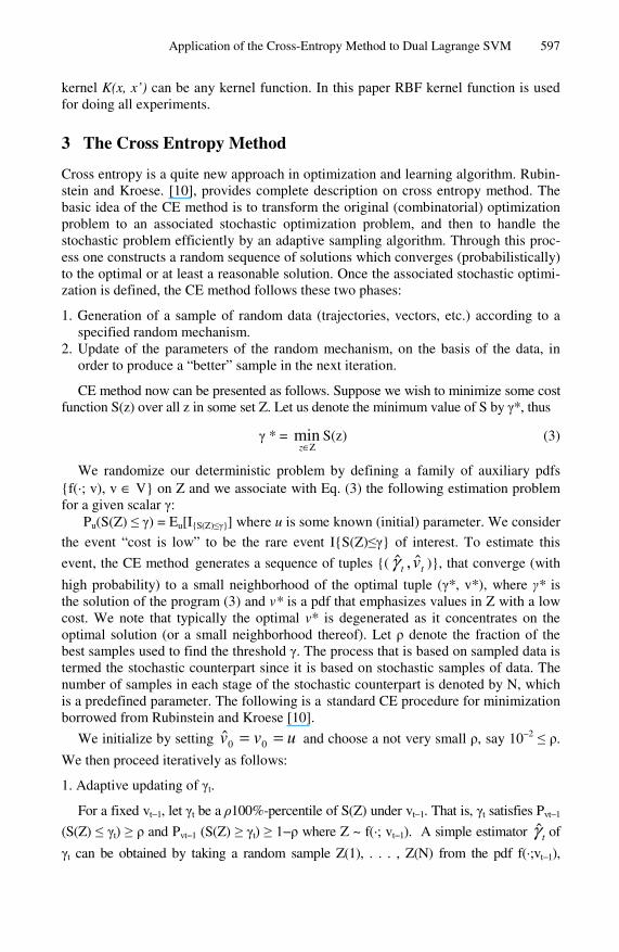
3 The Cross Entropy Method

Cross entropy is a quite new approach in optimization and learning algorithm. Rubin-stein and Kroese. [10], provides complete description on cross entropy method. The basic idea of the CE method is to transform the original (combinatorial) optimization problem to an associated stochastic optimization problem, and then to handle the stochastic problem efficiently by an adaptive sampling algorithm. Through this proc-ess one constructs a random sequence of solutions which converges (probabilistically) to the optimal or at least a reasonable solution. Once the associated stochastic optimi-zation is defined, the CE method follows these two phases:

1. Generation of a sample of random data (trajectories, vectors, etc.) according to a specified random mechanism.

2. Update of the parameters of the random mechanism, on the basis of the data, in order to produce a “better” sample in the next iteration.

CE method now can be presented as follows. Suppose we wish to minimize some cost function S(z) over all z in some set Z. Let us denote the minimum value of S by γ*, thus

γ * = Ζ∈z

min S(z) (3)

We randomize our deterministic problem by defining a family of auxiliary pdfs {f(·; v), v ∈ V} on Z and we associate with Eq. (3) the following estimation problem for a given scalar γ:

Pu(S(Z) ≤ γ) = Eu[I{S(Z)≤γ}] where u is some known (initial) parameter. We consider

the event “cost is low” to be the rare event I{S(Z)≤γ} of interest. To estimate this

event, the CE method generates a sequence of tuples {( tt v̂,γ̂ )}, that converge (with

high probability) to a small neighborhood of the optimal tuple (γ*, v*), where γ* is the solution of the program (3) and v* is a pdf that emphasizes values in Z with a low cost. We note that typically the optimal v* is degenerated as it concentrates on the optimal solution (or a small neighborhood thereof). Let ρ denote the fraction of the best samples used to find the threshold γ. The process that is based on sampled data is termed the stochastic counterpart since it is based on stochastic samples of data. The number of samples in each stage of the stochastic counterpart is denoted by N, which is a predefined parameter. The following is a standard CE procedure for minimization borrowed from Rubinstein and Kroese [10].

We initialize by setting uvv == 00ˆ and choose a not very small ρ, say 10−2 ≤ ρ.

We then proceed iteratively as follows:

1. Adaptive updating of γt.

For a fixed vt−1, let γt be a ρ100%-percentile of S(Z) under vt−1. That is, γt satisfies Pvt−1

(S(Z) ≤ γt) ≥ ρ and Pvt−1 (S(Z) ≥ γt) ≥ 1−ρ where Z ~ f(·; vt−1). A simple estimator tγ̂ of

γt can be obtained by taking a random sample Z(1), . . . , Z(N) from the pdf f(·;vt−1),

598 B. Santosa

calculating the performances S(Z(ℓ)) for all ℓ, ordering them from smallest to biggest as

S(1) ≤ . . . ≤ S(N) and finally evaluating the ρ100% sample percentile as tγ̂ = S([ρN]).

2. Adaptive updating of vt. For a fixed γt and vt−1, derive vt from the solution of the program

);(logmax)(max })({1 vZfIvD tZSvtvv

γ≤−Ε= (4)

The stochastic counterpart of (4) is as follows: for fixed tγ̂ and 1ˆ −tv , derive tv̂ from

the following program:

);(log1

max)(ˆmax )(

1}ˆ)({

vZfIN

vDN

tZSvv∑

=≤

= γ (5)

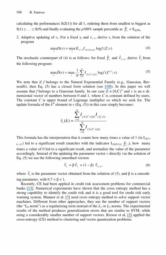
We note that if f belongs to the Natural Exponential Family (e.g., Gaussian, Ber-noulli), then Eq. (5) has a closed form solution (see [10]). In this paper we will assume that f belongs to a Gaussian family. In our case Z ∈{0,C}n and v is an n di-mensional vector of numbers between 0 and 1, where C is constant defined by users. The constant C is upper bound of Lagrange multiplier αs which we seek for. The update formula of the kth element in v (Eq. (5)) in this case simply becomes:

∑

∑

=≤

==≤

=N

tZS

N

ZtZS

t

I

IIkv

k

1}ˆ)({

1}1{}ˆ)({

)(ˆ

γ

γ

This formula has the interpretation that it counts how many times a value of 1 (in I{Z(ℓ)

k =1}) led to a significant result (matches with the indicator I{S(Z(ℓ))≤ tγ̂ }), how many

times a value of 0 led to a significant result, and normalize the value of the parameter accordingly. Instead of the updating the parameter vector v directly via the solution of Eq. (5) we use the following smoothed version

tv̂ = β tv̂ + (1 − β) 1ˆ −tv , (6)

where tv̂ is the parameter vector obtained from the solution of (5), and β is a smooth-

ing parameter, with 0.7 < β < 1. Recently, CE had been applied in credit risk assessment problems for commercial

banks [12]. Numerical experiments have shown that the cross entropy method has a strong capability to identify the credit risk and it is a good tool for credit risk early warning system. Mannor et al. [7] used cross entropy method to solve support vector machines. Different from other approaches, they use the number of support vectors (the “L0 norm”) as a regularizing term instead of the L1 or L2 norms. The experimental results of the method produces generalization errors that are similar to SVM, while using a considerably smaller number of support vectors. Kroese et al. [2] applied the cross-entropy (CE) method to clustering and vector quantization problems.

Application of the Cross-Entropy Method to Dual Lagrange SVM 599

4 The Proposed Approach

Adopting the idea of gradient ascent method on dual Lagrange SVM as applied in Kernel Adatron, the proposed approach, named CE-SVM, can be explained as follows. The method starts with generate N (number of samples) Lagrange multiplier, α and generate μ and σ values with the size N. Lagrange multiplier α represents Z and pa-rameters μ and σ functioned as v in Section 3. This vector α then inputted to the score function L as denoted in equation 2. L is functioned as S(z) in Section 3. The values of L are sorted descendently. Ne elite samples selected from the Ne smallest values of L. From these L values, the corresponding α can be identified. If of these α values <=0, as formulated in the second constraint in 2, set αi=0. If not, then we have to choose min(alpha,C). From the Ne α values, take the average and standard deviation and use smooth updated procedure to compute parameters μ and σ. Use this μ and σ to update α values in the next iteration. The same procedures are repeated until the parameter σ reach specified value epsilon. Fig 1 shows the pseudocode of CE-SVM algorithm. Input: pattern X, label Y, kernel function, kernel

parameter, C, Number of sample N and Number of elite sample Ne

Assign beta=1; Compute kernel Matrix K Compute H as y(i) * y(j) * K Generate initial random vector μ between [0,1],with size 1 x b (b is number of data points) Intialize vector σ=1 with size 1 x b while absolute value of (sum(σ)) > epsilon do,

For each data point, assign α=mu+σ*normally distribution random number For all sample points N

For all α do If α <=0 then set α =0

Else If α >C then set α =C EndIf

Endfor For all sample points N

Compute ∑∑∑== =

−=m

iiji

m

ij

m

jij xxKyL

11 12

1 αααα ),()(

Sort L in descending order Select α corresponding to Ne sample points with lowest L, and compute the average and standard deviation of these α values, denote as α and σ Update μ using μ = beta*α +(1-beta)*μ; Update σ using σ = beta*σ +(1-beta)*σ;

Endfor Output: α= μ

Fig. 1. Pseudocode for CE-SVM algorithm

600 B. Santosa

In this paper the following classifier is used

∑∈

=SVi

iii xxKysignxf ),(()( α

where α obtained from implementing algorithm CE-SVM which are nonzero (denoted as support vector, SV). Note that the bias b is not used in the classifier.

5 Experiments

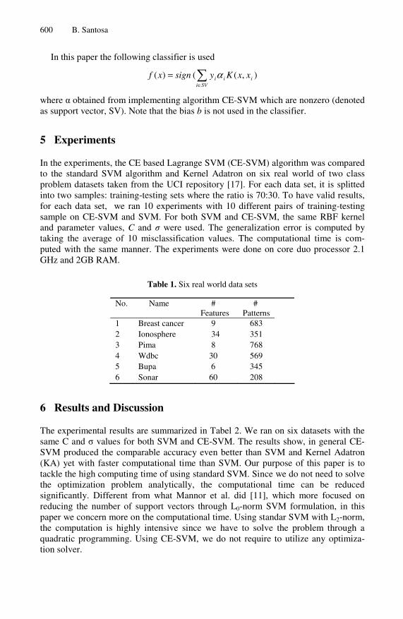
In the experiments, the CE based Lagrange SVM (CE-SVM) algorithm was compared to the standard SVM algorithm and Kernel Adatron on six real world of two class problem datasets taken from the UCI repository [17]. For each data set, it is splitted into two samples: training-testing sets where the ratio is 70:30. To have valid results, for each data set, we ran 10 experiments with 10 different pairs of training-testing sample on CE-SVM and SVM. For both SVM and CE-SVM, the same RBF kernel and parameter values, C and σ were used. The generalization error is computed by taking the average of 10 misclassification values. The computational time is com-puted with the same manner. The experiments were done on core duo processor 2.1 GHz and 2GB RAM.

Table 1. Six real world data sets

No. Name # Features

# Patterns

1 Breast cancer 9 683 2 Ionosphere 34 351 3 Pima 8 768 4 Wdbc 30 569 5 Bupa 6 345 6 Sonar 60 208

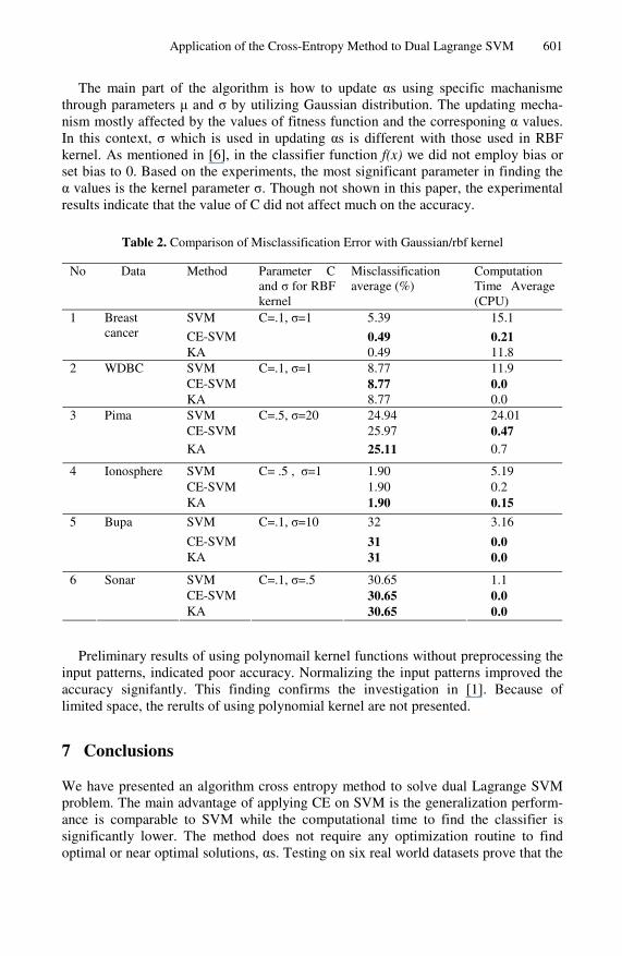
6 Results and Discussion

The experimental results are summarized in Tabel 2. We ran on six datasets with the same C and σ values for both SVM and CE-SVM. The results show, in general CE-SVM produced the comparable accuracy even better than SVM and Kernel Adatron (KA) yet with faster computational time than SVM. Our purpose of this paper is to tackle the high computing time of using standard SVM. Since we do not need to solve the optimization problem analytically, the computational time can be reduced significantly. Different from what Mannor et al. did [11], which more focused on reducing the number of support vectors through L0-norm SVM formulation, in this paper we concern more on the computational time. Using standar SVM with L2-norm, the computation is highly intensive since we have to solve the problem through a quadratic programming. Using CE-SVM, we do not require to utilize any optimiza-tion solver.

Application of the Cross-Entropy Method to Dual Lagrange SVM 601

The main part of the algorithm is how to update αs using specific machanisme through parameters μ and σ by utilizing Gaussian distribution. The updating mecha-nism mostly affected by the values of fitness function and the corresponing α values. In this context, σ which is used in updating αs is different with those used in RBF kernel. As mentioned in [6], in the classifier function f(x) we did not employ bias or set bias to 0. Based on the experiments, the most significant parameter in finding the α values is the kernel parameter σ. Though not shown in this paper, the experimental results indicate that the value of C did not affect much on the accuracy.

Table 2. Comparison of Misclassification Error with Gaussian/rbf kernel

No Data Method Parameter C and σ for RBF kernel

Misclassification average (%)

Computation Time Average (CPU)

SVM C=.1, σ=1 5.39 15.1

CE-SVM 0.49 0.21

1 Breast cancer

KA

0.49 11.8 SVM 8.77 11.9 CE-SVM 8.77 0.0

2 WDBC

KA

C=.1, σ=1

8.77 0.0 SVM 24.94 24.01 CE-SVM 25.97 0.47

3 Pima

KA

C=.5, σ=20

25.11 0.7

SVM 1.90 5.19 CE-SVM 1.90 0.2

4 Ionosphere

KA

C= .5 , σ=1

1.90 0.15

SVM 32 3.16

CE-SVM 31 0.0

5 Bupa

KA

C=.1, σ=10

31 0.0

SVM 30.65 1.1 CE-SVM 30.65 0.0

6 Sonar

KA

C=.1, σ=.5

30.65 0.0

Preliminary results of using polynomail kernel functions without preprocessing the

input patterns, indicated poor accuracy. Normalizing the input patterns improved the accuracy signifantly. This finding confirms the investigation in [1]. Because of limited space, the rerults of using polynomial kernel are not presented.

7 Conclusions

We have presented an algorithm cross entropy method to solve dual Lagrange SVM problem. The main advantage of applying CE on SVM is the generalization perform-ance is comparable to SVM while the computational time to find the classifier is significantly lower. The method does not require any optimization routine to find optimal or near optimal solutions, αs. Testing on six real world datasets prove that the

602 B. Santosa

proposed method shows promising results. More investigation by applying other kernels rather than RBF and other datasets might reveal interesting insight on the application of CE on SVM.

Acknowledgments. This research is supported by Higher Education Directorate of Indonesia Education Ministry 2008.

References

1. Chin, K.K.: Support Vector Machines applied to Speech Pattern Classification, Disserta-tion, Darwin College, University of Cambridge (1998)

2. Kroese, D.P., Rubinstein, R.Y., Taimre, T.: Application of the Cross-Entropy Method to Clustering and Vector Quantization. Journal of Machine Learning Research (2004)

3. Frieb, T.T., Christianini, N., Campbell, C.: The Kernel Adatron Algorithm: a Fast and Simple Learning Procedure for Support Vector Machines. In: Shavlik, J. (ed.) Proceedings of the 15th International Conference on Machine Learning, pp. 188–196. Morgan Kauf-mann, San Francisco (1998)

4. Hsu, C.W., Lin, C.J.: A Simple Decomposition Method for Support Vector Ma-chines 46(1-3), 291–314 (2002)

5. Joachims, T.: Making large-scale support vector machine learning practical. In: Advances in kernel methods: support vector learning. MIT Press, Cambridge (1999)

6. Kecman, V., Vogt, M., Huang, T.M.: On the Equality of Kernel AdaTron and Sequential Minimal Optimization in Classification and Regression Tasks and Alike Algorithms for Kernel Machines. In: ESANN 2003 proceedings, Belgium, pp. 215–222. d-side publi. (2003)

7. Mannor, S., Peleg, D., Rubinstein, R.Y.: The cross entropy method for classification. In: Proceedings of the 22nd International Conference on Machine Learning, Bonn, Germany (2005)

8. Platt, J.C.: Fast training of support vector machines using sequential minimal optimization. In: Advances in kernel methods: support vector learning, pp. 185–208. MIT Press, Cam-bridge (1999)

9. Rubinstein, R.Y.: Optimization of computer simulation models with rare events. European Journal of Operations Research 99, 89–112 (1997)

10. Rubinstein, R., Kroese, D.: The cross-entropy method: A unified approach to combinato-rial optimization, Monte-Carlo simulation, and machine-learning. Springer, Heidelberg (2004)

11. UCI Repository (2009), http://www.ics.uci.edu/~mlearn/mlrepository.html

12. Zhou, H., Wang, J., Qiu, Y.: Application of the Cross Entropy Method to the Credit Risk Assessment in an Early Warning System. In: International Symposiums on Information Processing (2008)