Noise-induced escape through a chaotic saddle: lowering of the activation energy

Physica D 181 (2003) 222–234

Noise-induced escape through a chaotic saddle:lowering of the activation energy

Suso Krauta,b,∗, Ulrike Feudelba Institut für Physik, Universität Potsdam, Postfach 601553, D-14415 Potsdam, Germany

b ICBM, Carl von Ossietzky Universität, PF 2503, 26111 Oldenburg, Germany

Received 19 December 2002; received in revised form 11 March 2003; accepted 21 March 2003Communicated by R. Roy

Abstract

The noise-induced escape mechanism is investigated for a prototype time-discrete nonequilibrium system describing alaser in a ring cavity with optical feedback, the Ikeda map. For certain parameter values a chaotic saddle is embedded in thebasin of attraction of the metastable state. This results in a lowering of the escape threshold for the activation energy, which isestablished by employing the theory of quasipotentials. Our findings are explained by the computation of themost probableexit path (MPEP), which lies partly on the chaotic saddle. The enhancement of escape turns out to be maximal if the MPEPlies entirely on the chaotic saddle.© 2003 Elsevier Science B.V. All rights reserved.

PACS: 05.45.−a; 05.40.Ca; 05.70.Ln; 42.60.Mi

Keywords: Chaotic saddle; Metastable; Activation energy

1. Introduction

Noise-induced escape over a potential barrier hasbeen studied extensively[1,2] since the seminal workby Kramers[3]. However, if the system under con-sideration is not in thermal equilibrium, as it was as-sumed in Kramers’ theory, many new features of theescape process can occur. Onsager and Machlup[4]realized that the escape process consists of large fluc-tuations, which are very rare, and that the trajectorypeaks sharply around some optimal, i.e. most proba-ble escape path (MPEP). Thus, despite the stochastic

∗ Corresponding author. Present address: Institut für Physik, Uni-versität Potsdam, Postfach 601553, D-14415 Potsdam, Germany.Tel.: +49-3319771364; fax:+49-3319771142.E-mail address: [email protected] (S. Kraut).

nature of the escape process, the escape path is almostdeterministic. Compared to the MPEP other paths havean exponentially smaller probability. That theory wasderived for a small noise levelσ → 0.

In the last years, it has become possible to performalso experiments on the escape problem, which in-clude Josephson junctions[5], electronic circuits[6],optical traps[7], lasers[8,9], and an electron in a Pen-ning trap[10].

Some of the most interesting novel theoreticalfindings include an understanding of the singularitiesof the nonequilibrium potential[11–14], a pre-expo-nential factor of the Kramers rate[15], a symmetrybreaking bifurcation of the MPEP[16] and a distri-bution of the escape paths originating from a cusppoint singularity[17]. Although in general the escape

0167-2789/03/$ – see front matter © 2003 Elsevier Science B.V. All rights reserved.doi:10.1016/S0167-2789(03)00098-8

S. Kraut, U. Feudel / Physica D 181 (2003) 222–234 223

occurs via a saddle point on the basin boundary (or alimit cycle), the very intriguing phenomenon of saddlepoint avoidance for a special system has been discov-ered[18]. Also a stepwise growth of the escape ratefor short time scales has been found[19]. Recently,an oscillation of the escape rate in dependence on thefriction for a multiwell potential was demonstrated[20]. For a fluctuating barrier the effect of resonantactivation has been theoretically predicted[21] andexperimentally confirmed[22]. Furthermore, the caseof colored noise has also been treated[23,24].

For nonadiabatically periodically driven systems anumber of interesting results has been obtained aswell, like a resonance decrease in the activation en-ergy [25], a logarithmic susceptibility of the fluctua-tion probability [26] and an enhancement of escapedue to transient chaos[27]. The calculation of the pref-actor was carried out in[28,29] and a complete ana-lytical solution for a moderatively strong driving fieldwas given in[30].

In this paper, we investigate the noise-induced es-cape process in a time-discrete version of an equationdescribing a laser system with time-delayed feedback,the Ikeda map. We have found in a previous investiga-tion a new mechanism of lowering the required energyfor noise-induced escape, i.e. an enhancement of es-cape, as a parameter is varied[31]. Thus the mean firstexit time is effectively reduced. This is achieved, if achaotic saddle is embedded in the open neighborhoodof a metastable state from which the trajectory escapesdue to noise. Here we explain in detail, especiallywith the help of the MPEP, how the enhancement ofescape is caused by the chaotic saddle. InSection 2we present the model, which is used to demonstratethe phenomenon andSection 3 gives an accountof the methods we employ, namely the theory ofquasipotentials, based on the Hamiltonian formalismby Freidlin and Wentzell[32]. Section 4demonstratesthe lowering of the escape energy due to the exis-tence of an embedded chaotic saddle. To understandthis phenomenon in more detail we compute the mostprobable exit path (MPEP) (Section 5) and show thatthe escape process in the presence of a chaotic saddleconsists of three steps: (i) ‘jump’ onto the saddle, (ii)motion on the saddle and (iii) ‘jump’ from the saddle

onto the basin boundary. The energy needed for thesethree steps is calculated related to the question of theminimal energy required to steer the system out ofthe metastable state (Section 6). Finally, we summa-rize our results inSection 7and compare them toother mechanisms of noise-induced enhancement ofescape.

2. The model

The noise-induced escape has previously been stud-ied using dissipative maps[33–35]. In many respects,time-discrete systems allow an analysis in a straight-forward way. Our model system is the Ikeda map[36].This is an idealized model of a laser pulse in an opti-cal cavity with time-delayed feedback. With complexvariables it has the form

zn+1 = a + bzn exp

[iκ − iη

1 + |zn|2]

, (1)

wherezn = xn + iyn is related to the amplitude andphase of thenth laser pulse exiting the cavity. All theparameters are real,a is the laser input amplitude andcorresponds to the external forcing of the system. Thedamping (1− b) accounts for the reflection propertiesof the mirrors in the cavity and measures the dissipa-tion. The empty cavity detuning is given byκ and thedetuning due to a nonlinear dielectric medium byη.The Ikeda map gives rise to rich dynamical behavior, itexhibits for some parameters even highly multistablebehavior[37,38].

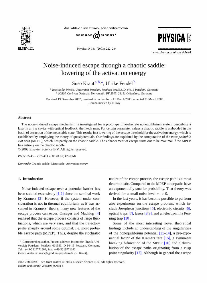
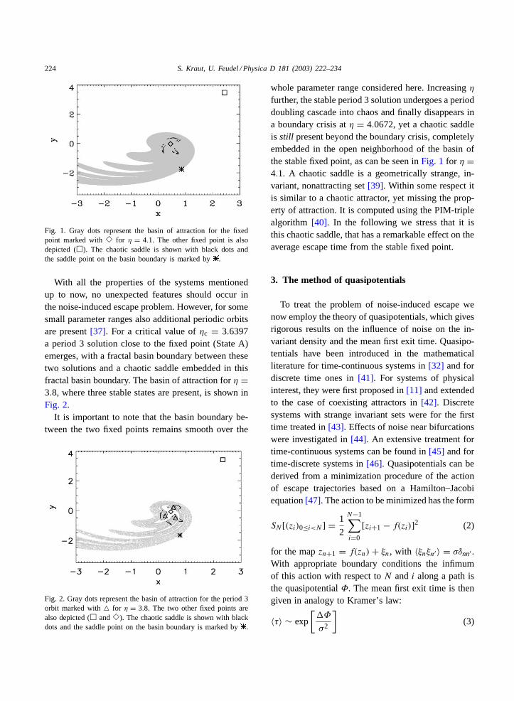
We fix the parameters ata = 0.85, b = 0.9 andκ = 0.4 and vary onlyη in the range 2.6 < η < 12.For the noiseless system two stable states are present.One fixed point (State A,� in Fig. 1) undergoes aperiod doubling scenario and becomes a chaotic at-tractor atη ≈ 5.17. Another fixed point (State B,�in Fig. 1) remains a fixed point over the whole pa-rameter range considered. We focus on the investiga-tion of the noise-induced escape from State A. Thebasin boundary separating these two stable states is asmooth curve, which is built by the stable manifoldof the saddle point C ( in Fig. 1), separating the twostable states.

224 S. Kraut, U. Feudel / Physica D 181 (2003) 222–234

Fig. 1. Gray dots represent the basin of attraction for the fixedpoint marked with� for η = 4.1. The other fixed point is alsodepicted (�). The chaotic saddle is shown with black dots andthe saddle point on the basin boundary is marked by.

With all the properties of the systems mentionedup to now, no unexpected features should occur inthe noise-induced escape problem. However, for somesmall parameter ranges also additional periodic orbitsare present[37]. For a critical value ofηc = 3.6397a period 3 solution close to the fixed point (State A)emerges, with a fractal basin boundary between thesetwo solutions and a chaotic saddle embedded in thisfractal basin boundary. The basin of attraction forη =3.8, where three stable states are present, is shown inFig. 2.

It is important to note that the basin boundary be-tween the two fixed points remains smooth over the

Fig. 2. Gray dots represent the basin of attraction for the period 3orbit marked with� for η = 3.8. The two other fixed points arealso depicted (� and�). The chaotic saddle is shown with blackdots and the saddle point on the basin boundary is marked by.

whole parameter range considered here. Increasingη

further, the stable period 3 solution undergoes a perioddoubling cascade into chaos and finally disappears ina boundary crisis atη = 4.0672, yet a chaotic saddleis still present beyond the boundary crisis, completelyembedded in the open neighborhood of the basin ofthe stable fixed point, as can be seen inFig. 1 for η =4.1. A chaotic saddle is a geometrically strange, in-variant, nonattracting set[39]. Within some respect itis similar to a chaotic attractor, yet missing the prop-erty of attraction. It is computed using the PIM-triplealgorithm [40]. In the following we stress that it isthis chaotic saddle, that has a remarkable effect on theaverage escape time from the stable fixed point.

3. The method of quasipotentials

To treat the problem of noise-induced escape wenow employ the theory of quasipotentials, which givesrigorous results on the influence of noise on the in-variant density and the mean first exit time. Quasipo-tentials have been introduced in the mathematicalliterature for time-continuous systems in[32] and fordiscrete time ones in[41]. For systems of physicalinterest, they were first proposed in[11] and extendedto the case of coexisting attractors in[42]. Discretesystems with strange invariant sets were for the firsttime treated in[43]. Effects of noise near bifurcationswere investigated in[44]. An extensive treatment fortime-continuous systems can be found in[45] and fortime-discrete systems in[46]. Quasipotentials can bederived from a minimization procedure of the actionof escape trajectories based on a Hamilton–Jacobiequation[47]. The action to be minimized has the form

SN [(zi)0≤i<N ] = 1

2

N−1∑i=0

[zi+1 − f(zi)]2 (2)

for the mapzn+1 = f(zn) + ξn, with 〈ξnξn′ 〉 = σδnn′ .With appropriate boundary conditions the infimumof this action with respect toN and i along a path isthe quasipotentialΦ. The mean first exit time is thengiven in analogy to Kramer’s law:

〈τ〉 ∼ exp

[�Φ

σ2

](3)


with �Φ defined as the minimal quasipotential dif-ference

�Φ := inf {Φ(y) − Φ(a) : a ∈ A, y ∈ ∂G}, (4)

whereA is the attractor and∂G is the basin boundary.The numerical computations of the quasipotentials areperformed on a grid, using the Dijkstra algorithm toobtain the lowest energy on the grid[48]. Starting fromthe grid point, where the fixed point is located, we as-sign to each neighboring grid point a value which isdetermined by the cost function(1/2)[zi+1 − f(zi)]2.This value can be considered as a measure of the de-viation from the deterministic dynamics between thegrid points. Then the closest point (i.e. the one withthe lowest cost function) of all the neighbors is cho-sen as a new starting point. In turn, all neighbors ofthe new point, which are not among the closest pointsyet, are updated again. For all points treated so far apredecessor list is built, which shows the shortest wayto the starting point. This goes on, until the last pointhas been chosen. In the end, a certain value has beenassigned to each grid point and the minimization overN has been performed automatically. The point, whichis located on the basin boundary and which has thelowest value yields the minimal escape energy. Hispredecessor list gives the escape path. In principle, thealgorithm is able to reveal the predicted singularties inthe quasipotential[11–14]. However, it would require

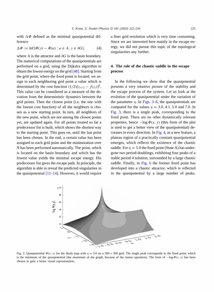
Fig. 3. QuasipotentialΦ(x, y) for the Ikeda map withη = 3.0 on a 300× 300 grid. The single peak corresponds to the fixed point, whichis the minimum of the quasipotential (the maximum of the graph, because of the minus operation). The form of−logΦ(x, y) has beenchosen to gain a better visual representation.

a finer grid resolution which is very time consuming.Since we are interested here mainly in the escape en-ergy, we did not pursue this topic of the topologicalsingularities any further.

4. The role of the chaotic saddle in the escapeprocess

In the following we show that the quasipotentialpresents a very intuitive picture of the stability andthe escape process of the system. Let us look at theevolution of the quasipotential under the variation ofthe parameterη. In Figs. 3–6, the quasipotentials arecomputed for the valuesη = 3.0, 4.1, 5.0 and 7.0. InFig. 3, there is a single peak, corresponding to thefixed point. There are no other dynamically relevantproperties, hence−logΦ(x, y) (this form of the plotis used to get a better view of the quasipotential) de-creases in every direction. InFig. 4, as a new feature, aplateau region of a practically constant quasipotentialemerges, which reflects the existence of the chaoticsaddle. Forη = 5.0 the fixed point (State A) has under-gone two period-doublings, exhibiting four peaks of astable period 4 solution, surrounded by a large chaoticsaddle. Finally, inFig. 6 the former fixed point hasdeveloped into a chaotic attractor, which is reflectedin the quasipotential by a large number of peaks.


Fig. 4. QuasipotentialΦ(x, y) for the Ikeda map withη = 4.1 on a 300× 300 grid. The single peak corresponds again to the fixed point.Also, an extended plateau at−logΦ(x, y) ≈ 5.0 is visible, caused by the chaotic saddle.

Actually, every point on the chaotic attractor shouldbe represented by a peak, which is, though, not visi-ble here due to the finite spatial resolution. Again theplateau of the chaotic saddle is visible slightly belowthe attractor corresponding to slightly smaller valuesof −logΦ(x, y).

To use the quasipotential for the noise-induced es-cape problem, the minimum value ofΦ(x, y) on thebasin boundary has to be determined, according toEq. (4). This is exactly the minimum escape energy�Φ(x, y), since the quasipotential at the stable solu-tion (fixed point, periodic orbit or chaotic attractor) is

Fig. 5. QuasipotentialΦ(x, y) for the Ikeda map withη = 5.0 on a 300× 300 grid. The four peaks correspond to a period 4 attractor. Theplateau at−logΦ(x, y) ≈ 7.5 is due to a very large chaotic saddle.

zero by definition. The point on the basin boundarywith minimal quasipotential (escape energy) is gener-ally a saddle point of the system[49]. This is also thecase for the Ikeda map, as shown inFig. 7.

In order to quantify the escape process with thequasipotential, we plot for various values ofη the cor-responding minimal escape energy�Φ(x, y) in Fig. 8.A pronounced nonmonotonic behavior is visible. Thefirst local maximum of the curve is at the value ofη ≈3.6, where the chaotic saddle comes into existence. Toelucidate the role of the chaotic saddle as the originof an enhancement of noise-induced escape, we also


Fig. 6. QuasipotentialΦ(x, y) for the Ikeda map withη = 7.0 on a 300× 300 grid. The complex peak structure corresponds to a chaoticattractor. Again, an extended plateau at−logΦ(x, y) ≈ 7.0 slightly below the attractor is visible, caused by the chaotic saddle.

include in the plot the value of the height of the plateauin the quasipotential. For all values ofη ≥ 3.6397 wehave computed the chaotic saddle, except forη = 5.5.Therefore, it is not clear whether there exists a chaoticsaddle forη = 5.5 or not. The PIM-triple method, aswell as the quasipotential, yield forη = 5.5 no conclu-sive result, as a chaotic saddle may existvery close tothe chaotic attractor and numerically it is very difficultto distinguish between the two. Since the chaotic sad-dle can be computed forη-values smaller and biggerthanη = 5.5 we expect the saddle to exist also for thisvalue, even though the numerical check remained un-conclusive. The escape energies were also computed

Fig. 7. Contour plot ofFig. 4 at the minimal value of thequasipotentialΦ(x, y), where it touches the basin boundary,−logΦ(x, y) = 4.915 (the basin of attraction of the other attrac-tor is shown in gray). The saddle point on the basin boundary isshown as .

using straightforward Monte Carlo simulations yield-ing the same results within the numerical error.

To see the effect of the chaotic saddle on the min-imal escape energy more clearly, it is important toquantify the influence of the relative size of the basinof attraction, since it is increasing with increasingη

and we are here only interested in the change of theminimal escape energy caused by the chaotic saddle.The distance between the attractor and the saddle pointon the boundary is usually proportional to the rela-tive size of the basin. Both quantities are expected toplay a role in the stability of the metastable state lo-cated in the basin, although we are not aware of anytheoretical work dealing with this relation directly. To

Fig. 8. Minimal escape energy (log�Φ(x, y), �) and height of thesaddle plateau in the quasipotential (log�Φ(saddle), �) versusη.


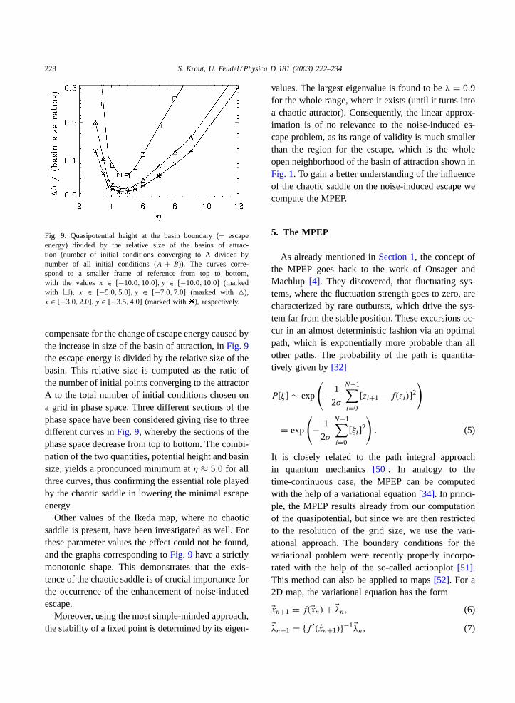
Fig. 9. Quasipotential height at the basin boundary (= escapeenergy) divided by the relative size of the basins of attrac-tion (number of initial conditions converging to A divided bynumber of all initial conditions (A + B)). The curves corre-spond to a smaller frame of reference from top to bottom,with the valuesx ∈ [−10.0, 10.0], y ∈ [−10.0, 10.0] (markedwith �), x ∈ [−5.0, 5.0], y ∈ [−7.0, 7.0] (marked with �),x ∈ [−3.0, 2.0], y ∈ [−3.5, 4.0] (marked with ), respectively.

compensate for the change of escape energy caused bythe increase in size of the basin of attraction, inFig. 9the escape energy is divided by the relative size of thebasin. This relative size is computed as the ratio ofthe number of initial points converging to the attractorA to the total number of initial conditions chosen ona grid in phase space. Three different sections of thephase space have been considered giving rise to threedifferent curves inFig. 9, whereby the sections of thephase space decrease from top to bottom. The combi-nation of the two quantities, potential height and basinsize, yields a pronounced minimum atη ≈ 5.0 for allthree curves, thus confirming the essential role playedby the chaotic saddle in lowering the minimal escapeenergy.

Other values of the Ikeda map, where no chaoticsaddle is present, have been investigated as well. Forthese parameter values the effect could not be found,and the graphs corresponding toFig. 9 have a strictlymonotonic shape. This demonstrates that the exis-tence of the chaotic saddle is of crucial importance forthe occurrence of the enhancement of noise-inducedescape.

Moreover, using the most simple-minded approach,the stability of a fixed point is determined by its eigen-

values. The largest eigenvalue is found to beλ = 0.9for the whole range, where it exists (until it turns intoa chaotic attractor). Consequently, the linear approx-imation is of no relevance to the noise-induced es-cape problem, as its range of validity is much smallerthan the region for the escape, which is the wholeopen neighborhood of the basin of attraction shown inFig. 1. To gain a better understanding of the influenceof the chaotic saddle on the noise-induced escape wecompute the MPEP.

5. The MPEP

As already mentioned inSection 1, the concept ofthe MPEP goes back to the work of Onsager andMachlup [4]. They discovered, that fluctuating sys-tems, where the fluctuation strength goes to zero, arecharacterized by rare outbursts, which drive the sys-tem far from the stable position. These excursions oc-cur in an almost deterministic fashion via an optimalpath, which is exponentially more probable than allother paths. The probability of the path is quantita-tively given by[32]

P [ξ] ∼ exp

(− 1

2σ

N−1∑i=0

[zi+1 − f(zi)]2

)

= exp

(− 1

2σ

N−1∑i=0

[ξi]2

). (5)

It is closely related to the path integral approachin quantum mechanics[50]. In analogy to thetime-continuous case, the MPEP can be computedwith the help of a variational equation[34]. In princi-ple, the MPEP results already from our computationof the quasipotential, but since we are then restrictedto the resolution of the grid size, we use the vari-ational approach. The boundary conditions for thevariational problem were recently properly incorpo-rated with the help of the so-called actionplot[51].This method can also be applied to maps[52]. For a2D map, the variational equation has the form

�xn+1 = f(�xn) + �λn, (6)

�λn+1 = {f ′(�xn+1)}−1�λn, (7)


where�xn is the state vector of the 2D mapf and�λn isthe 2D Lagrangian multiplier. To solve this equationnumerically, we now employ the technique of the ac-tionplot [51,52], which is a refined shooting method.The exact initial conditions have to be chosen in sucha way, that�x0 is distributed on a small circle with ra-dius l and angleφ around the stable solution�xfix, and�λn points in the unstable direction of the fixed point.The iteration of the variational equation terminates, if�xn has left the basin of attraction (which is checked bysimply forward iterating�xn for eachn with the orig-inal equations). The proper initial conditions l andφ

are those, which minimize∑N

i=0�λ2i and thusEq. (2).

They provide the MPEP. However, the structure of theactionplot is fractal[51,52]and it has many local min-ima, which can make it a very difficult task to find theoverall minimum and thus the MPEP.

The MPEP forη = 3.0 is presented inFig. 10. It isspiraling out of the metastable solution, comes closerto the basin boundary, until it is hitting it exactly atthe saddle point, in full agreement with the theory.

An important new feature appears forη = 4.1,where the chaotic saddle is present, as demonstrated inFig. 11. The escape process consists of three steps inthis case, namely, a noise-induced fluctuation from theattractor (State A) to the chaotic saddle, then movingalong points of it and finally from the chaotic saddleto the saddle point on the boundary. As will be ex-plained below, it is the motion on points of the chaotic

Fig. 10. Optimal escape path forη = 3.0 shown with (�), con-nected with lines to guide the eyes. The saddle point on the bound-ary is shown with and the basin for the other stable solutionshown in gray.

Fig. 11. Optimal escape path forη = 4.1 shown with (�), con-nected with lines to guide the eyes. The chaotic saddle is shownwith black dots and the saddle point on the boundary with; thebasin for the other stable solution is shown in gray.

saddle, which results in a lowering of the escape en-ergy, since it consumes (in principle) no energy, as thewhole chaotic saddle has the same height (in terms ofenergy) in the quasipotential. In our example, sincethere is some steering necessary to decrease the over-all escape energy and an optimal exit on the saddlehas to be found to jump close to the basin boundary,also the motion on the saddle needs energy, but it isat least one order of magnitude smaller than without asaddle (compareFigs. 13–15). Thus�Φ(x, y) is closeto zero and very little external force is required.

Fig. 12. Optimal escape path forη = 5.0 shown with (�), con-nected with lines to guide the eyes. The chaotic saddle is shownwith black dots and the saddle point on the boundary with; thebasin for the other stable solution is shown in gray.


This fact explains also the maximal enhancementof escape observed inFig. 9 for η = 5.0. The opti-mal escape path for this value is depicted inFig. 12.The chaotic saddle is much more extended. This re-sults in an enlarged coincidence of the escape pathand points on the chaotic saddle, which means thatfor most of the path almost no energy is needed. Thewhole escape process can be viewed as consisting ba-sically of two steps requiring energy: the first ‘jump’from the metastable State A to the chaotic saddleand the second ‘jump’ from the chaotic saddle to thesaddle point on the boundary. The relation betweenthe escape path and the energy needed for each stepon this path is discussed in more detail in the nextsection.

6. Escape energy and control

To get a deeper understanding of the MPEP andthe corresponding required escape energy, we show inthis section how the escape energy relates to the exitpath. This is also relevant for control considerations,as has been stressed in[53,54], since the MPEP, andthe corresponding fluctuational force give the minimal

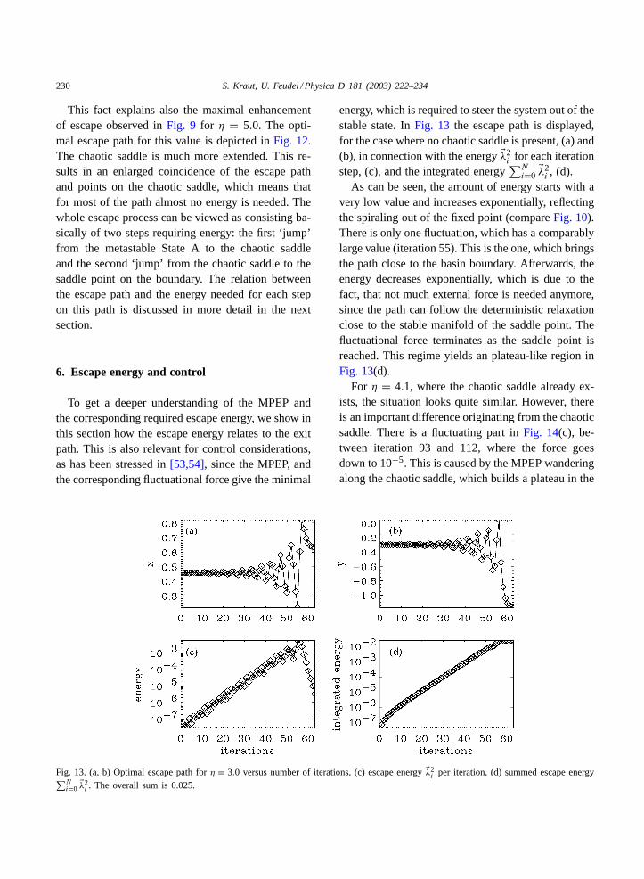
Fig. 13. (a, b) Optimal escape path forη = 3.0 versus number of iterations, (c) escape energy�λ2i per iteration, (d) summed escape energy∑N

i=0�λ2i . The overall sum is 0.025.

energy, which is required to steer the system out of thestable state. InFig. 13 the escape path is displayed,for the case where no chaotic saddle is present, (a) and(b), in connection with the energy�λ2

i for each iterationstep, (c), and the integrated energy

∑Ni=0

�λ2i , (d).

As can be seen, the amount of energy starts with avery low value and increases exponentially, reflectingthe spiraling out of the fixed point (compareFig. 10).There is only one fluctuation, which has a comparablylarge value (iteration 55). This is the one, which bringsthe path close to the basin boundary. Afterwards, theenergy decreases exponentially, which is due to thefact, that not much external force is needed anymore,since the path can follow the deterministic relaxationclose to the stable manifold of the saddle point. Thefluctuational force terminates as the saddle point isreached. This regime yields an plateau-like region inFig. 13(d).

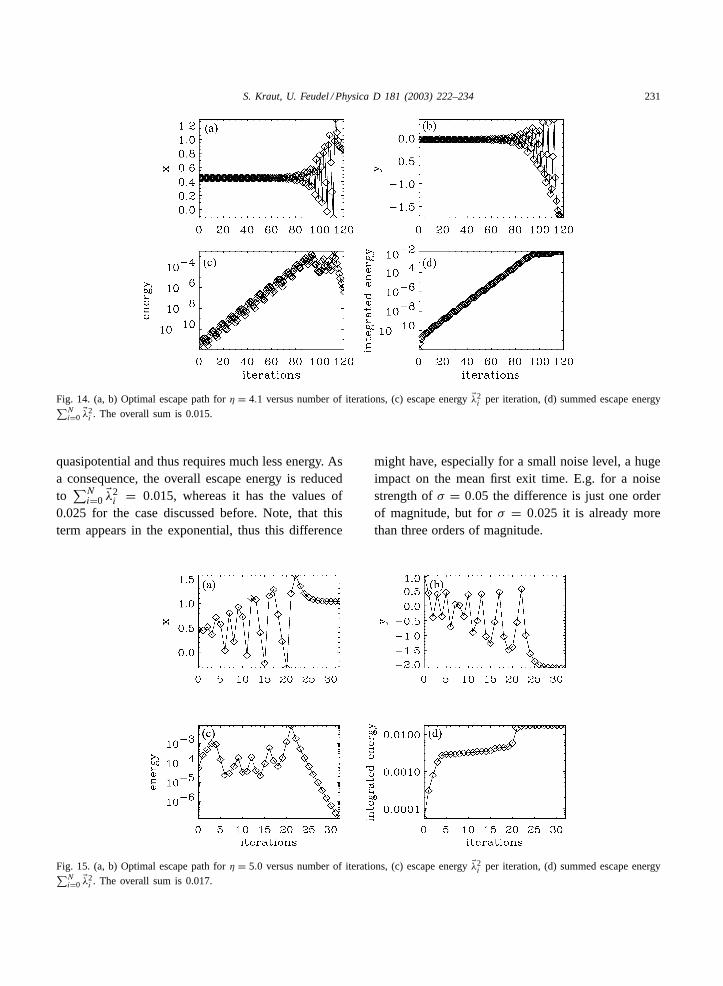
For η = 4.1, where the chaotic saddle already ex-ists, the situation looks quite similar. However, thereis an important difference originating from the chaoticsaddle. There is a fluctuating part inFig. 14(c), be-tween iteration 93 and 112, where the force goesdown to 10−5. This is caused by the MPEP wanderingalong the chaotic saddle, which builds a plateau in the




quasipotential and thus requires much less energy. Asa consequence, the overall escape energy is reducedto∑N

i=0�λ2i = 0.015, whereas it has the values of

0.025 for the case discussed before. Note, that thisterm appears in the exponential, thus this difference



might have, especially for a small noise level, a hugeimpact on the mean first exit time. E.g. for a noisestrength ofσ = 0.05 the difference is just one orderof magnitude, but forσ = 0.025 it is already morethan three orders of magnitude.


As could already be expected fromFig. 12, the mostdistinct behavior takes place forη = 5.0, shown inFig. 15. There is no exponential increase in the fluc-tuational force, see (c), as the MPEP starts directly onthe chaotic saddle. After some iterations on points ofthe chaotic saddle, the optimal fluctuation of iteration21, which is 10 times larger than all others, transportsagain the path near the boundary and in the followingthe needed energy falls off exponentially, as before.The chaotic saddle has the maximal effect here, whichis also seen in the large plateau, between iteration 5and 20, inFig. 15(d). The energy hardly grows, sincethe MPEP lies on the chaotic saddle and only a mini-mal amount of external input is necessary.

It is important to note that the number of iterationsfor η = 5.0 is the least, since the MPEP approaches thesaddle right at the start. The overall escape energy is∑N

i=0�λ2i = 0.017. This is larger as forη = 4.1, which

is, however, only caused by the growth of the basinof attraction. Compensating this effect, the minimumoccurs forη = 5.0, as discussed above in connectionwith Fig. 9. The enhancement of escape through achaotic saddle is most strikingly demonstrated forη =5.0 for the following two reasons. First, the MPEP isalready after the first iterations on the chaotic saddleand almost no fluctuations are required to approachit. Secondly, all iterations of the MPEP until the pathcomes close to the boundary lie on the chaotic sad-dle and demand only little energy, because the saddlecorresponds to a plateau in the quasipotential. In anysituation, where these two conditions are met, the en-hancement is maximal. Further increasingη results ina period doubling of the stable state, which becomeschaotic forη ≈ 5.17. At the same time, the chaoticsaddle shrinks again. We did not compute MPEPs forthis parameter region, due to the following complica-tions: if the stable solution is a chaotic attractor, it isnot a priori known which point on the attractor has tobe chosen as the initial condition for the variationalequation. Although there is some preliminary work fora quasiattractor[55] and the Lorenz attractor[56,57],no general solution exits for this problem. However,since the maximal enhancement occurs forη = 5.0,where the attractor is still periodic, the phenomenonpresented here is not affected by these difficulties.

7. Summary and discussion

We have demonstrated the effect of enhancementof noise-induced escape through the existence ofa chaotic saddle in the open neighborhood of themetastable state as a parameter is varied. Employingthe theory of quasipotentials and the related conceptof the MPEP, it was possible to understand this low-ering of the escape threshold. Our results are, thoughdemonstrated for the Ikeda map, of general validity,and can in principle be found in a large variety ofsystems. The mechanism of the escape process relieson the existence of a chaotic saddle embedded in theopen neighborhood of the metastable state. It consistsof three steps, namely, a noise-induced fluctuationfrom the attractor (State A) to the chaotic saddle, awandering on this chaotic saddle, and finally a fluctu-ation from the chaotic saddle to the fixed point (StateB) via the saddle point on the boundary (State C).The enhancement is maximal, if the chaotic saddleis most extended. Then the first step is negligibleand the second, which is the essential mechanism toescape, becomes crucial. In a successful escape, thechaotic saddle acts as a ‘shortcut’, since its presencelowers the overall escape energy. For small noise lev-els, which are still experimentally feasible, though,the influence on the mean first exit time can be sev-eral orders of magnitude. It should thus be possibleto confirm our findings also in experiments.

We stress that the reported mechanism of the low-ering of the escape energy is qualitatively differentfrom a recently found effect, where also an enhance-ment of noise-induced escape through transient mo-tion (typical for chaotic saddles) has been found by[27]. In their scenario, a nonadiabatically, periodicallydriven system exhibits a facilitation of noise-inducedinterwell transitions. This occurs, because the basinboundary becomes fractal and the distance betweenthe two states is effectively reduced. In the mechanismreported here we always have a smooth basin bound-ary between the two stable states and the chaotic sad-dle is embedded in the basin of one state, not in thebasin boundary between the states.

It is further important to note that the escape processis more complex than in the situation, when the MPEP


just passes through a single unstable periodic orbit(UPO), which is embedded in the basin of attraction[53,55]. Since a chaotic saddle is made of an infinitenumber of UPOs[58,59], one might expect, that in ourcase the MPEP passes through one or a collection ofUPOs of the chaotic saddle. However, we computedall UPOs of low period and could not find any onelying on the MPEP. This fact led us to conclude thatthe chaotic saddle acts in an even stronger way than aunion of UPOs of different low periods could do. Thuswe speculate that the enhancement would not be sopronounced, if the chaotic saddle would be replaced byan even very high number of UPOs with low periods.

Acknowledgements

We acknowledge A. Hamm, D. Luchinsky and S.Beri for valuable discussions and A. Hamm also forthe help in programming. This work was supported bythe DFG and INTAS.

References

[1] P. Hänggi, P. Talkner, M. Borkovec, Rev. Mod. Phys. 62(1990) 251.

[2] V.I. Mel’nikov, Phys. Rep. 209 (1991) 1.[3] H.A. Kramers, Physica 7 (1940) 287.[4] L. Onsager, S. Machlup, Phys. Rev. 91 (1953) 1505;

L. Onsager, S. Machlup, Phys. Rev. 91 (1953) 1512.[5] D. Vion, M. Götz, P. Joyez, D. Esteve, M.H. Devoret, Phys.

Rev. Lett. 77 (1996) 3435.[6] D.G. Luchinsky, P.V.E. McClintock, Nature (London) 389

(1997) 463.[7] L.I. McCann, M. Dykman, B. Golding, Nature (London) 402

(1999) 785.[8] J. Hales, A. Zhukov, R. Roy, M.I. Dykman, Phys. Rev. Lett.

85 (2000) 78.[9] M.B. Willemsen, M.U.F. Khalid, M.P. van Exter, J.P.

Woerdman, Phys. Rev. Lett. 82 (1999) 4815.[10] L.J. Lapidus, D. Enzer, G. Gabrielse, Phys. Rev. Lett. 83

(1999) 899.[11] R. Graham, T. Tel, Phys. Rev. Lett. 52 (1984) 9.[12] H.R. Jauslin, Physica A 144 (1987) 179.[13] M.I. Dykman, M.M. Millonas, V.N. Smelyanskiy, Phys. Lett.

A 195 (1994) 53.[14] R.S. Maier, D.L. Stein, Phys. Rev. Lett. 77 (1996) 4860.[15] R.S. Maier, D.L. Stein, Phys. Rev. Lett. 69 (1992) 3691;

P. Reimann, E. Lootens, Europhys. Lett. 34 (1996) 1.[16] R.S. Maier, D.L. Stein, Phys. Rev. Lett. 71 (1993) 1783.

[17] M.I. Dykman, D.G. Luchinsky, P.V.E. McClintock, V.N.Smelyanskiy, Phys. Rev. Lett. 77 (1996) 5229.

[18] D.G. Luchinsky, R.S. Maier, R. Mannella, P.V.E. McClintock,D.L. Stein, Phys. Rev. Lett. 82 (1999) 1806.

[19] S.M. Soskin, V.I. Sheka, T.L. Linnik, R. Mannella, Phys. Rev.Lett. 86 (2001) 1665.

[20] S.M. Soskin, J. Stat. Phys. 97 (1999) 609;M. Arrayás, I.Kh. Kaufman, D.G. Luchinsky, P.V.E.McClintock, S.M. Soskin, Phys. Rev. Lett. 84 (2000) 2556.

[21] C.R. Doering, J.C. Gadoua, Phys. Rev. Lett. 69 (1992) 2318.[22] R.N. Mantegna, B. Spagnolo, Phys. Rev. Lett. 76 (1996) 563.[23] A.J. Bray, A.J. McKane, Phys. Rev. Lett. 62 (1989) 493.[24] M.I. Dykman, Phys. Rev. A 42 (1990) 2020.[25] M.I. Dykman, H. Rabitz, V.N. Smelyanskiy, B.E. Vugmeister,

Phys. Rev. Lett. 79 (1997) 1178.[26] V.N. Smelyanskiy, M.I. Dykman, H. Rabitz, B.E. Vugmeister,

Phys. Rev. Lett. 79 (1997) 3113.[27] S.M. Soskin, R. Mannella, M. Arrayás, A.N. Silchenko, Phys.

Rev. E 63 (2001) 051111.[28] J. Lehmann, P. Reimann, P. Hänggi, Phys. Rev. Lett. 84

(2000) 1639;J. Lehmann, P. Reimann, P. Hänggi, Phys. Rev. E 62 (2000)6282.

[29] R.S. Maier, D.L. Stein, Phys. Rev. Lett. 86 (2001) 3942.[30] V.N. Smelyanskiy, M.I. Dykman, B. Golding, Phys. Rev. Lett.

82 (1999) 3193;V.N. Smelyanskiy, M.I. Dykman, H. Rabitz, B.E. Vugmeister,S.L. Bernasek, A.B. Bocarsly, J. Chem. Phys. 23 (1999)11488.

[31] S. Kraut, U. Feudel, Phys. Rev. E 67 (2003) 015204.[32] M.I. Freidlin, A.D. Wentzell, Random Perturbations of

Dynamical Systems, Springer-Verlag, Berlin, 1984.[33] P.D. Beale, Phys. Rev. A 40 (1989) 3998.[34] P. Grassberger, J. Phys. A 22 (1989) 3283.[35] P. Reimann, P. Talkner, Phys. Rev. E 51 (1995) 4105.[36] K. Ikeda, Opt. Commun. 30 (1979) 257;

S. Hammel, C.K.R.T. Jones, J. Maloney, J. Opt. Soc. Am. B2 (1985) 552.

[37] Y.-C. Lai, C. Gebogi, J.A. Yorke, in: J.H. Kim, J. Stringer(Eds.), Applied Chaos, Wiley, New York, 1992, p. 441.

[38] U. Feudel, C. Grebogi, Chaos 7 (1997) 597.[39] T. Tél, in: Hao Bai-lin (Ed.), Directions in Chaos, vol. 4,

World Scientific, Singapore, 1990, pp. 149–211.[40] H.E. Nusse, J.A. Yorke, Physica D 36 (1989) 137.[41] Y. Kifer, Random Perturbations of Dynamical Systems,

Birkhäuser, Boston, 1988.[42] R. Graham, T. Tél, Phys. Rev. A 33 (1986) 1322.[43] R. Graham, A. Hamm, T. Tél, Phys. Rev. Lett. 66 (1991)

3089.[44] A. Hamm, T. Tél, R. Graham, Phys. Lett. A 185 (1994) 313.[45] R. Graham, in: F. Moss, P.V.E. McClintock (Eds.), Noise in

Nonlinear Dynamical Systems, 3 volumes, vol. 1, CambridgeUniversity Press, Cambridge, 1989, pp. 225–278.

[46] A. Hamm, R. Graham, J. Stat. Phys. 66 (1992) 689.[47] P. Talkner, P. Hänggi, E. Freidkin, D. Trautmann, J. Stat.

Phys. 48 (1987) 231.[48] A.V. Aho, J.D. Ullman, J.E. Hopcroft, Data Structures and

Algorithms, Addison-Wesley, Reading, MA, 1983.


[49] M. Dykman, M.A. Krivoglaz, Sov. Phys. JETP 50 (1979) 30.[50] R.P. Feynman, A.R. Hibbs, Quantum Mechanics and Path

Integrals, McGraw-Hill, New York, 1965;L.S. Schulman, Techniques and Applications of PathIntegration, Wiley, New York, 1981.

[51] S. Beri, D.G. Luchinsky, R. Mannella, P.V.E. McClintock,submitted for publication.

[52] S. Beri, S. Kraut, I.A. Khovanov, D.G. Luchinsky, P.V.E.McClintock, in preparation.

[53] I.A. Khovanov, D.G. Luchinsky, R. Mannella, P.V.E.McClintock, Phys. Rev. Lett. 85 (2000) 2100.

[54] D.G. Luchinsky, S. Beri, R. Mannella, P.V.E. McClintock,I.A. Khovanov, Int. J. Bif. Chaos 12 (2002) 583.

[55] D.G. Luchinsky, I.A. Khovanov, JETP Lett. 69 (1999) 825.[56] V.S. Anishchenko, I.A. Khovanov, N.A. Khovanova, D.G.

Luchinsky, P.V.E. McClintock, Fluct. Noise Lett. 1 (2001)L27.

[57] V.S. Anishchenko, D.G. Luchinsky, P.V.E. McClintock, I.A.Khovanov, N.A. Khovanova, JETP 94 (2002) 821.

[58] D. Auerbach, P. Cvitanovic, J.-P. Eckmann, G. Gunaratne, I.Procaccia, Phys. Rev. Lett. 58 (1987) 2387.

[59] C. Grebogi, E. Ott, J.A. Yorke, Phys. Rev. A 37 (1988) 1711.

Noise-induced escape through a chaotic saddle: lowering of the activation energy

Documents

Transcript of Noise-induced escape through a chaotic saddle: lowering of the activation energy