Optimality and uniqueness of the Leech lattice among lattices
39
arXiv:math/0403263v2 [math.MG] 30 Sep 2008 OPTIMALITY AND UNIQUENESS OF THE LEECH LATTICE AMONG LATTICES HENRY COHN AND ABHINAV KUMAR Dedicated to Oded Schramm (10 December 1961 – 1 September 2008) Abstract. We prove that the Leech lattice is the unique densest lattice in R 24 . The proof combines human reasoning with computer verification of the prop- erties of certain explicit polynomials. We furthermore prove that no sphere packing in R 24 can exceed the Leech lattice’s density by a factor of more than 1+1.65 · 10 -30 , and we give a new proof that E 8 is the unique densest lattice in R 8 . 1. Introduction It is a long-standing open problem in geometry and number theory to find the densest lattice in R n . Recall that a lattice Λ ⊂ R n is a discrete subgroup of rank n; a minimal vector in Λ is a nonzero vector of minimal length. Let |Λ| = vol(R n /Λ) denote the covolume of Λ, i.e., the volume of a fundamental parallelotope or the absolute value of the determinant of a basis of Λ. If r is the minimal vector length of Λ, then spheres of radius r/2 centered at the points of Λ do not overlap except tangentially. This construction yields a sphere packing of density π n/2 (n/2)! r 2 n 1 |Λ| , since the volume of a unit ball in R n is π n/2 /(n/2)!, where for odd n we define (n/2)! = Γ(n/2 + 1). The densest lattice in R n is the lattice for which this quantity is maximized. There might be several distinct densest lattices in the same dimension. For example, the greatest density known in R 25 is achieved by at least 23 distinct lattices, although they are not known to be optimal. (See pages xix and 178 of [CS2] for the details.) We will speak of “the densest lattice” because it sounds more natural. The problem of finding the densest lattice is a special case of the sphere packing problem, but there is no reason to believe that the densest sphere packing should come from a lattice. In particular, in R 10 the densest packing known is the Best packing P 10c , which is not a lattice packing (see [CS2, p. 140]), and it is conjectured that lattices are suboptimal in all sufficiently high dimensions. However, many of the most interesting packings in low dimensions are lattice packings, and lattices have strong connections with other fields such as number theory. For example, the Hermite constant γ n is defined to be the smallest constant such that for every Date : September 27, 2008. Kumar was supported by a summer internship in the Theory Group at Microsoft Research and by a Putnam graduate fellowship at Harvard University. 1
-
Upload
independent -
Category
Documents
-
view
6 -
download
0
Transcript of Optimality and uniqueness of the Leech lattice among lattices

arX
iv:m
ath/
0403
263v
2 [
mat
h.M
G]
30
Sep
2008
OPTIMALITY AND UNIQUENESS OF THE LEECH LATTICE
AMONG LATTICES
HENRY COHN AND ABHINAV KUMAR
Dedicated to Oded Schramm (10 December 1961 – 1 September 2008)
Abstract. We prove that the Leech lattice is the unique densest lattice in R24.
The proof combines human reasoning with computer verification of the prop-erties of certain explicit polynomials. We furthermore prove that no spherepacking in R
24 can exceed the Leech lattice’s density by a factor of more than1 + 1.65 · 10−30, and we give a new proof that E8 is the unique densest latticein R
8.
1. Introduction
It is a long-standing open problem in geometry and number theory to find thedensest lattice in R
n. Recall that a lattice Λ ⊂ Rn is a discrete subgroup of rank n;
a minimal vector in Λ is a nonzero vector of minimal length. Let |Λ| = vol(Rn/Λ)denote the covolume of Λ, i.e., the volume of a fundamental parallelotope or theabsolute value of the determinant of a basis of Λ. If r is the minimal vector lengthof Λ, then spheres of radius r/2 centered at the points of Λ do not overlap excepttangentially. This construction yields a sphere packing of density
πn/2
(n/2)!
(r
2
)n 1
|Λ| ,
since the volume of a unit ball in Rn is πn/2/(n/2)!, where for odd n we define
(n/2)! = Γ(n/2+1). The densest lattice in Rn is the lattice for which this quantity
is maximized.There might be several distinct densest lattices in the same dimension. For
example, the greatest density known in R25 is achieved by at least 23 distinct
lattices, although they are not known to be optimal. (See pages xix and 178 of[CS2] for the details.) We will speak of “the densest lattice” because it soundsmore natural.
The problem of finding the densest lattice is a special case of the sphere packingproblem, but there is no reason to believe that the densest sphere packing shouldcome from a lattice. In particular, in R
10 the densest packing known is the Bestpacking P10c, which is not a lattice packing (see [CS2, p. 140]), and it is conjecturedthat lattices are suboptimal in all sufficiently high dimensions. However, many ofthe most interesting packings in low dimensions are lattice packings, and latticeshave strong connections with other fields such as number theory. For example,the Hermite constant γn is defined to be the smallest constant such that for every
Date: September 27, 2008.Kumar was supported by a summer internship in the Theory Group at Microsoft Research and
by a Putnam graduate fellowship at Harvard University.
1

2 HENRY COHN AND ABHINAV KUMAR
positive-definite quadratic form Q(x1, . . . , xn) of determinant D, there is a nonzerovector (v1, . . . , vn) ∈ Z
n such that Q(v1, . . . , vn) ≤ γnD1/n. Finding the maximumdensity of a lattice packing in R
n is equivalent to computing γn.The densest lattice in R
n is known for n ≤ 8: the answers are the root latticesA1, A2, A3, D4, D5, E6, E7, and E8. For n = 3 this is due to Gauss [G], for4 ≤ n ≤ 5 to Korkine and Zolotareff [KZ1, KZ2], and for 6 ≤ n ≤ 8 to Blichfeldt[Bl]. However, before the present paper no further cases had been solved since 1935.In 1946 Chaundy claimed to have dealt with n = 9 and n = 10, but his paper [Ch]implicitly assumes that a densest lattice in R
n must contain one in Rn−1 as a cross
section. That is known to be false (see [CS1]), so the paper appears irreparablyflawed.
In each of the solved cases, the optimal lattice is furthermore known to be unique,up to scaling and isometries. This was proved simultaneously with the optimalityfor n ≤ 5, for n = 6 it was proved by Barnes [Ba], and for 6 ≤ n ≤ 8 it was provedby Vetcinkin [Ve].
In this paper we deal with n = 24 (the theorem numbering is as it will appearlater in the paper):
Theorem 9.3. The Leech lattice is the unique densest lattice in R24, up to scaling
and isometries of R24.
In terms of the Hermite constant, γ24 = 4. We also give a new proof for E8:
Theorem 11.7 (Blichfeldt, Vetcinkin). The E8 root lattice is the unique densest
lattice in R8, up to scaling and isometries of R
8.
Our work is motivated by the paper [CE] by Cohn and Elkies (see also [Co]),which proves upper bounds for the sphere packing density. In particular, the maintheorem in [CE] is an analogue for sphere packing of the linear programming boundsfor error-correcting codes: given a function satisfying certain linear inequalities onecan deduce a density bound. It is not known how to choose the function to optimizethe bound, but in R
8 and R24 one can come exceedingly close to the densities of
E8 and the Leech lattice, respectively. This observation, together with analogieswith error-correcting codes and spherical codes, led Cohn and Elkies to conjecturethat their bound is sharp in R
8 and R24, which would solve the sphere packing
problem in those dimensions. While we cannot yet fully carry out that program,in this paper we show how to combine the methods of [CE] with results on latticesand combinatorics to deal with the special case of lattice packings. We will dealprimarily with the Leech lattice, because that case is new and more difficult, butin Section 11 we will discuss E8.
One might hope to use a relatively simple method. Section 8 of [CE] shows howto prove that the Leech lattice is the unique densest periodic packing (i.e., unionof finitely many translates of a lattice) in R
24, if a function from R24 to R with
certain properties exists. Using a computer, one can find functions that very nearlyhave those properties, and the techniques from Section 8 of [CE] can then be usedstraightforwardly to prove an approximate version of the uniqueness result: everylattice that is at least as dense as the Leech lattice must be close to it. It is known(see [Ma, p. 176]) that the Leech lattice is a strict local optimum for density, amonglattices. Thus, if one can show that every denser lattice is sufficiently close, then itproves that the Leech lattice is the unique densest lattice in R
24.

OPTIMALITY AND UNIQUENESS OF THE LEECH LATTICE AMONG LATTICES 3
Unfortunately, this approach seems completely infeasible if carried out in themost straightforward way. When one naively imitates the techniques from Section 8of [CE] in an approximate setting, one loses a tremendous factor in the bounds,and that puts the required computer searches far beyond what we are capable of.In this paper we salvage the approach by using more sophisticated arguments thattake advantage of special properties of the Leech lattice. In particular, we makeuse of three beautiful facts about the Leech lattice: its automorphism group actstransitively on pairs of minimal vectors with the same inner product, its minimalvectors form an association scheme when pairs are grouped according to their innerproducts, and its minimal vectors form a spherical 11-design. (Note that the secondproperty follows from the first, but our work uses another proof of it, from [DGS].)
Our proof depends on computer calculations in some places, but they can becarried out relatively quickly, in less than one hour using a personal computer. Thecalculations are all done using exact arithmetic and are thus rigorous. We havefully documented all of our calculations and made available commented code foruse in checking the results or carrying out further investigations. See Appendix Afor details.
Appendix B contains very brief introductions to several topics: the Leech lattice,linear programming bounds, spherical designs, and association schemes. For moredetails, see [CS2]. The expository article [E2] also provides useful background andcontext, although it does not include everything we need.
2. Outline of proof
We wish to show that the Leech lattice, henceforth denoted by Λ24, is the uniquedensest sphere packing among all lattices in R
24. Let Λ be any lattice in R24 that is
at least as dense as Λ24. Without loss of generality, we assume that Λ has covolume1. Then the restriction on its density simply means its minimal vectors have lengthat least 2.
We first show, using linear programming bounds, that Λ has exactly 196560vectors of length approximately 2 (called nearly minimal vectors), and that the
next smallest vector length is approximately√
6.We rescale those 196560 nearly minimal vectors to lie on the unit sphere. Then
they form a spherical code with minimal angle at least ϕ, where cosϕ is very near to(and greater than or equal to) 1/2. Note that in S23 there is a unique spherical codeof this size with minimal angle π/3 = cos−1(1/2), and it is the kissing arrangementof Λ24; the spherical code derived from Λ should be a small perturbation of thisconfiguration.
Using linear programming bounds, we show that the inner products of the unitvectors are approximately 0,±1/4,±1/2,±1. We prove that if pairs of vectors aregrouped according to their inner products, then they form an association schemewith the same valencies and intersection numbers as in the case of Λ24, and thatit must therefore be the same association scheme. This isomorphism gives us acorrespondence between minimal vectors of Λ24 and nearly minimal vectors of Λ,such that corresponding inner products are approximately equal.
Using this correspondence, we find a basis of Λ whose Gram matrix is close tothe Gram matrix of a basis of Λ24. Finally, from the strict local optimality of theLeech lattice we conclude that Λ must in fact be the Leech lattice.

4 HENRY COHN AND ABHINAV KUMAR
3. Notation
We begin by recording our normalizations of some special functions (which arealways as in [AAR]), and defining some notation.
The Laguerre polynomials Lαi (z) are defined by the initial conditions Lα
0 (z) = 1and Lα
1 (z) = 1 + α − z and the recurrence
iLαi (z) = (2i − 1 + α − z)Lα
i−1(z) − (i + α − 1)Lαi−2(z)
for i ≥ 2. They are orthogonal polynomials with respect to the measure e−xxα dx
on [0,∞). If α = n/2−1, then the functions on Rn given by x 7→ e−π|x|2Lα
i (2π|x|2)form an orthogonal basis of the radial functions in L2(Rn), and they are also eigen-functions of the Fourier transform with eigenvalue (−1)i (see (4.20.3) in [Leb]).Here we normalize the Fourier transform by
f(t) =
∫
Rn
f(x)e2πi〈x,t〉 dx.
Note also that with this normalization of the Fourier transform, the Poisson sum-mation formula states that
∑
x∈Λ
f(x) =1
|Λ|∑
t∈Λ∗
f(t),
if f : Rn → R is a Schwartz function, Λ ⊂ R
n is a lattice, and
Λ∗ = {y ∈ Rn : 〈x, y〉 ∈ Z for all x ∈ Λ}
is its dual lattice. (See (28) in [K, p. 49].)The ultraspherical (or Gegenbauer) polynomials Cλ
i (z) are defined by the initialconditions Cλ
0 (z) = 1 and Cλ1 (z) = 2λz and the recurrence
iCλi (z) = 2(i + λ − 1)zCλ
i−1(z) − (i + 2λ − 2)Cλi−2(z)
for i ≥ 2. They are orthogonal polynomials with respect to the measure
(1 − x2)λ−1/2 dx
on [−1, 1]. When λ = n/2−1, that measure is proportional to the projection of thesurface measure from Sn−1 onto an axis, and the ultraspherical polynomials playa fundamental role in the theory of spherical harmonics in R
n. Up to scaling, the
ultraspherical polynomial Cλi is the same as the Jacobi polynomial P
(α,α)i , where
α = λ − 1/2.Whenever we use Laguerre or ultraspherical polynomials, we will always set
α = λ = n/2 − 1, where n = 24 in the Leech lattice proof and n = 8 in the E8
proof. The term “ultraspherical coefficient” will mean a coefficient in the expansionof a polynomial as a linear combination of ultraspherical polynomials.
Throughout this paper, Λ24 will denote the Leech lattice, and Λ will denote anylattice in R
24 that is at least as dense and satisfies |Λ| = 1 (except in Section 9,where Λ denotes an arbitrary lattice, and in Section 11, which deals with E8). Wethink of Λ as being an optimal lattice, but we will not use that assumption. Wedo not even need to know a priori that a global optimum for density is achieved,although [GL, §17.5] shows that it is.
Whenever f : Rn → R is a radial function and r ∈ [0,∞), we will write f(r) for
the common value f(x) with x ∈ Rn satisfying |x| = r.

OPTIMALITY AND UNIQUENESS OF THE LEECH LATTICE AMONG LATTICES 5
The surface volume of the unit sphere Sn−1 ⊂ Rn will be denoted by
vol(Sn−1) = nπn/2
(n/2)!.
It is important to keep in mind that vol(Sn−1) is not the volume of the enclosedball.
We will make use of the numerical values
ε = 6.733 · 10−27,
µ = 3.981 · 10−13,
ν = 3.219 · 10−12, and
ω = 1.703 · 10−11
throughout the paper. Each will be defined the first time it is used, but we have col-lected the values here for easy reference. Note that terminating decimal expansionssuch as these represent exact rational numbers, not floating point approximations.
4. Nearly minimal vectors
In this section, we show that Λ must have exactly 196560 vectors of length near 2(this will be made more precise below). The first subsection examines which vectorlengths are possible in Λ, and the second then counts the nearly minimal vectors.
4.1. Restrictions on the lengths of vectors. Let f : R24 → R be a radial
Schwartz function with the following properties: f(0) = f(0) = 1, f(x) ≤ 0 for
|x| ≥ r (for some number r), and f(t) ≥ 0 for all t. Proposition 3.2 of [CE] saysthat if such a function exists, then the sphere packing density in R
24 is boundedabove by
π12
12!
( r
2
)24
.
If we could find such a function with r = 2, then it would prove that Λ24 has thegreatest density among all sphere packings in R
24, not just lattice packings. Cohnand Elkies conjecture that such a function exists, but the best they achieve in [CE]is r ≤ 2 · 1.00002946.
Our proof begins by constructing an explicit function f with
r ≤ 2(1 + 6.851 · 10−32
).
Note that the existence of such a function proves that no sphere packing in R24 can
have density greater than 1 + 1.65 · 10−30 times the density of Λ24.Unfortunately, the function we construct is extremely complicated (it would take
far too much space to write it down here). It consists of a polynomial of degree
803 with rational coefficients, evaluated at 2π|x|2 and multiplied by e−π|x|2. Itwas constructed by a lengthy computer calculation to optimize the value of r usingNewton’s method, and even verifying that it has the properties used below requiresa computer, although fortunately that is much easier than finding the function. Theaccompanying computer file verifyf.txt includes code to verify all the assertionsabout f in this subsection of the paper. See Appendix A for details.
We can use techniques similar to those in [CE] to study the size of the shortvectors in Λ. First, we need two lemmas. Set
ε = 6.733 · 10−27,

6 HENRY COHN AND ABHINAV KUMAR
and call a nonzero vector in Λ nearly minimal if it has length at most 2(1+ε). Thereason for this choice of ε will be apparent from Proposition 4.3 below.
Consider what happens if we rescale the nearly minimal vectors so that they alllie on the unit sphere. These vectors determine a spherical code
CΛ = {u/|u| : u a nearly minimal vector}on the unit sphere S23, and the following lemma bounds its minimal angle. (SeeAppendix B for background on spherical codes.)
Lemma 4.1. If u and v are nearly minimal vectors with u 6= v, then the angle ϕbetween u and v satisfies
cosϕ ≤ 1 − 1
2(1 + ε)2.
Proof. We have |u|, |v| ∈ [2, 2(1 + ε)] and |u − v| ≥ 2. By the law of cosines,
cosϕ =|u|2 + |v|2 − |u − v|2
2|u||v| ≤ |u|2 + |v|2 − 4
2|u||v| .
The bound (|u|2+|v|2−4)/(2|u||v|) is convex as a function of |u| and |v| individually,and hence it is maximized at one of the vertices of the square [2, 2(1+ ε)]2. In fact,the maximum occurs when |u| = |v| = 2(1 + ε), in which case the bound becomes
1 − 1
2(1 + ε)2.
�
Lemma 4.2. There are at most 196560 nearly minimal vectors in Λ.
Proof. This lemma is a straightforward application of the linear programmingbounds for spherical codes (see Chapter 9 of [CS2], or Appendix B for a briefsummary). Let
fε(x) = Kε(x + 1)
(x +
1
2
)2(x +
1
4
)2
x2
(x − 1
4
)2 (x −
(1 − 1
2(1 + ε)2
)),
where the constant Kε is chosen so that fε has zeroth ultraspherical coefficient 1.(The normalization is irrelevant for this proof, but it will be important later in thepaper, so we use it here for consistency.) If ε were 0, this polynomial would be theone used to solve the kissing problem exactly in R
24 (see Chapter 13 of [CS2]). Withthe current value of ε, the polynomial fε has nonnegative ultraspherical coefficientsand still proves that there are fewer than 196561 spheres in any spherical code inR
24 with minimal angle as in Lemma 4.1. (We check this assertion in the computerfile verifyrest.txt. In fact, the bound is less than 196560 + 10−19.) Thus, therecan be at most 196560 nearly minimal vectors in Λ. �
In addition to the definition of ε above, set
µ = 3.981 · 10−13,
ν = 3.219 · 10−12, and
ω = 1.703 · 10−11.
Proposition 4.3. Every nonzero vector in Λ has length in[2, 2(1 + ε)
)∪(√
6(1− µ),√
6(1 + µ))∪(√
8(1− ν),√
8(1 + ν))∪(√
10(1−ω),∞).

OPTIMALITY AND UNIQUENESS OF THE LEECH LATTICE AMONG LATTICES 7
Proof. By the Poisson summation formula,∑
x∈Λ
f(x) =∑
t∈Λ∗
f(t).
Because Λ is at least as dense as Λ24 (and has covolume 1), all nonzero vectorsx ∈ Λ satisfy |x| ≥ 2. Because r ≤ 2(1 + ε), by Lemma 4.2 there can be at most196560 vectors in Λ with 2 ≤ |x| ≤ r. Within that range, f is a decreasing functionof the radius, and we have
196560f(2) < 1.644104221 · 10−30
(recall from Section 3 that f(2) denotes the common value f(x) with |x| = 2).
The key properties of f are f(0) = f(0) = 1, f(x) ≤ 0 for |x| ≥ r, and f(t) ≥ 0for all t. It follows that
1 + 1.644104221 · 10−30 +∑
x∈N
f(x) ≥ 1,
where N is the set of vectors in Λ at which f is negative. No vector in Λ can occurwithin any region on which f is less than (1/2)(−1.644104221) · 10−30; the extrafactor of 2 comes from the fact that f(−x) = f(x) since f is a radial function (ifx ∈ N then −x ∈ N as well). That rules out all radii in the set
[2(1 + ε),
√6(1 − µ)
]∪[√
6(1 + µ),√
8(1 − ν)]∪[√
8(1 + ν),√
10(1 − ω)].
In the computer file verifyf.txt we prove this by examining the radial derivativeof f . �
Much of the rest of the proof would still work if ε, µ, ν, and ω were somewhatlarger. The two main places where they must be small are the final inequality (9.4)and the intersection number calculations in Subsection 6.2 (as well as the boundsused there). In each case they could be slightly larger, but not by a factor of 100.
4.2. 196560 nearly minimal vectors. We can now show that there are exactly196560 nearly minimal vectors. We know from Lemma 4.2 that there are at most196560 of them. For the other direction, a lower bound greater than 196559, weneed a new kind of linear programming bound. Recall that we have shown thatall nonzero vectors in Λ are either nearly minimal or have lengths greater than√
6(1 − µ).Suppose we knew that all nonzero vectors either have length exactly 2 or at least√
6. (We will first explain our method under these overly optimistic hypotheses.Lemma 4.4 will then apply it using the actual bounds we have proved.) One mighthope to count the nearly minimal vectors using a Schwartz function g : R
24 → R
such that g(x) ≤ 0 for |x| ≥√
6, g(t) ≥ 0 for all t, and g(2) > 0. Given such afunction, Poisson summation implies that
∑
x∈Λ
g(x) =∑
t∈Λ∗
g(t),
and hence
g(0) + Ng(2) ≥ g(0)
if there are N minimal vectors. Thus, N ≥ (g(0)− g(0))/g(2). We conjecture thatg can be chosen so that (g(0) − g(0))/g(2) = 196560, which is the largest possiblevalue because the Leech lattice has 196560 minimal vectors. We can construct

8 HENRY COHN AND ABHINAV KUMAR
functions that come quite close to this bound, and will use one of them to provethe following lemma.
Lemma 4.4. There are more than 196559 nearly minimal vectors in Λ.
Proof. Define z1, . . . , z10 by zi = ⌊4π(i+1)108⌋/108. In other words, they have thefollowing values:
i 1 2 3 4 5zi 25.13274122 37.69911184 50.26548245 62.83185307 75.39822368
i 6 7 8 9 10zi 87.96459430 100.53096491 113.09733552 125.66370614 138.23007675
There are unique coefficients a1, . . . , a37 such that
1 +37∑
i=1
aiL11i (x)
has a single root at z2 and a double root at zi for i ≥ 3, and
1 +
37∑
i=1
(−1)iaiL11i (x)
has a double root at each zi for i ≥ 1. Neither polynomial has any other nonnegativeroots. (We check this in the computer file verifyg.txt using Sturm’s theorem,except that we do not check the uniqueness of the coefficients because we do notrequire it.)
Define g : R24 → R by
g(x) =
(1 +
37∑
i=1
aiL11i (2π|x|2)
)e−π|x|2.
It follows that
g(t) =
(1 +
37∑
i=1
(−1)iaiL11i (2π|x|2)
)e−π|x|2.
We have g(x) ≤ 0 for |x| ≥√
6(1 − µ), because z2 < 2π · 6(1 − µ)2, the function gchanges sign only at z2, and g(0) > 0. For all t, we have g(t) ≥ 0.
Apply Poisson summation to g, to deduce∑
x∈Λ
g(x) =∑
t∈Λ∗
g(t).
Applying the two inequalities above shows that
g(0) +∑
x∈M
g(x) ≥ g(0),
where M is the set of nearly minimal vectors. The function g(x) is positive and adecreasing function of |x| on the interval [2, 2(1 + ε)], so
g(0) + |M|g(2) ≥ g(0).
However,g(0) − g(0)
g(2)> 196559,

OPTIMALITY AND UNIQUENESS OF THE LEECH LATTICE AMONG LATTICES 9
so there are more than 196559 nearly minimal vectors. (All these inequalities arechecked in verifyg.txt.) �
Thus, there must be exactly 196560 nearly minimal vectors, as desired. Weconjecture that this method could be used to recover each of the coefficients of theLeech lattice’s theta series, but we will not need that for our proof.
5. Inner products in the spherical code
We now continue to study the polynomial
fε(x) = Kε(x + 1)
(x +
1
2
)2(x +
1
4
)2
x2
(x − 1
4
)2(x −
(1 − 1
2(1 + ε)2
))
from the previous section.Note that
1 − 1
2(1 + ε)2<
1
2+ ε.
Thus, all the inner products except 1 in the spherical code CΛ are at most 1/2 + ε.We seek bounds for how far from 0,±1/4,±1/2,±1 they can be. The ±1 casesmust be exact, because of Lemma 4.1 and the fact that u ∈ CΛ iff −u ∈ CΛ (i.e.,the code is antipodal).
Because the zeroth ultraspherical coefficient of fε is 1, it follows from the usualproof of the linear programming bounds for spherical codes (see Appendix B) that
196560fε(1) +∑
x 6=y
fε(〈x, y〉) ≥ 1965602,
where the sum is over vectors in the spherical code. Because the four inner products〈x, y〉, 〈−x,−y〉, 〈y, x〉, and 〈−y,−x〉 are all equal, and all the terms in the sumare nonpositive, we see that no term in the sum can be less than
1965602 − 196560fε(1)
4,
which is approximately −1.99 · 10−15.Now a short calculation implies that all the inner products must be within 6.411 ·
10−9 of one of the numbers 0,±1/4,±1/2,±1. The exponent is only 9 because fε hasdouble roots, and one can stray quite far from a double root without substantiallychanging the function’s value.
In the rest of the paper, we make the following definition: let
σ = maxu,v∈CΛ
min{|〈u, v〉 − α| : α ∈ S},
where S = {0,±1/4,±1/2,±1}. In other words, σ is the maximum “error” in theinner products. We have just shown that σ ≤ 6.411 · 10−9. We will improve theupper bound for σ substantially, and ultimately we will show σ = 0.
5.1. Better bounds for σ. Recall that we computed in Section 4.1 that vectorsof Λ with length close to
√6 must have length in the interval
√6(1−µ),
√6(1+µ).
Therefore if we have nearly minimal vectors u, v with 〈u, v〉 ≈ 1 (with error less
than 10−3, say), then we see that |u − v| ≈√
6. Therefore
6(1 − µ)2 ≤ 〈u, u〉 + 〈v, v〉 − 2〈u, v〉 ≤ 6(1 + µ)2.

10 HENRY COHN AND ABHINAV KUMAR
In addition we have
4 ≤ 〈u, u〉 ≤ 4(1 + ε)2.
Therefore
8 − 6(1 + µ)2 ≤ 2〈u, v〉 ≤ 8(1 + ε)2 − 6(1 − µ)2,
so4 − 3(1 + µ)2
4(1 + ε)2≤⟨
u
|u| ,v
|v|
⟩≤ (1 + ε)2 − 3
4(1 − µ)2.
Similarly we get for 〈u, v〉 ≈ 0 that
1 − (1 + ν)2
(1 + ε)2≤⟨
u
|u| ,v
|v|
⟩≤ (1 + ε)2 − (1 − ν)2,
and for 〈u, v〉 ≈ 2 that
2 − (1 + ε)2
2(1 + ε)2≤⟨
u
|u| ,v
|v|
⟩≤ (1 + ε)2 − 1
2
because 2 ≤ |u − v| ≤ 2(1 + ε). Combining these (and if necessary replacing vwith −v), we find that for u 6= ±v, the inner product 〈u/|u|, v/|v|〉 differs from anelement of {0,±1/4,±1/2} by at most 6.43801 · 10−12. We conclude that the errorσ in the inner products is at most 6.43801 · 10−12.
However, we will be able to get much better bounds in Section 7, once we haveshown that the spherical code CΛ gives us an association scheme.
6. Association schemes
We would like to turn the 196560 points in the spherical code CΛ into a 6-classassociation scheme by grouping pairs according to their approximate inner products.(See Appendix B for background on association schemes.) It is not clear that this infact defines an association scheme, but we will show that it does. Furthermore, wewill show that this association scheme is isomorphic to the one derived from Λ24. Toachieve this, we show that the intersection numbers are the same as in Λ24. Thatwill also show that it is an association scheme, by showing that the intersectionnumbers are independent of the pair of points. We use the same techniques as[DGS], but we need to keep track of error bounds.
6.1. Spherical design. First, we show that CΛ is nearly a spherical 10-design.(See Appendix B for background on spherical designs.) Let
Ci(x) =C11
i (x)
C11i (1)
·(22+i22
)+(21+i22
)
vol(S23).
The advantage of this normalization of the ultraspherical polynomials is that forevery finite subset C of S23,
∑
x,y∈C
Ci(〈x, y〉) =
∣∣∣∣∣∑
z∈C
evi(z)
∣∣∣∣∣
2
,
where evi(z) denotes the evaluation at z map in the dual space to the i-th degreespherical harmonics. Although this fact is well known (e.g., it is equivalent toTheorem 9.6.3 in [AAR]), we will explain it here for completeness, because thecorrect normalization is important for our application.

OPTIMALITY AND UNIQUENESS OF THE LEECH LATTICE AMONG LATTICES 11
Lemma 6.1. If C is a finite subset of S23, then
∑
x,y∈C
Ci(〈x, y〉) =
∣∣∣∣∣∑
z∈C
evi(z)
∣∣∣∣∣
2
.
Proof. Let d be the dimension of the space of spherical harmonics of degree i, andlet S1, . . . , Sd be an orthonormal basis of that space. By Theorem 9.6.3 of [AAR],
d∑
j=1
Sj(w)Sj(z) = Ci(〈w, z〉).
Let f =∑
j ajSj be any spherical harmonic of degree i. Then
(evi(z))(f) =
d∑
j=1
ajSj(z)
=
d∑
j=1
Sj(z)
∫
S23
Sj(w)f(w) dw
=
∫
S23
d∑
j=1
Sj(w)Sj(z)
f(w) dw
=
∫
S23
Ci(〈w, z〉)f(w) dw.
Thus, (∑
z∈C
evi(z)
)(f) =
∫
S23
(∑
z∈C
Ci(〈w, z〉))
f(w) dw.
In other words, applying the element∑
z∈C evi(z) of the dual space is the same astaking the inner product with
w 7→∑
z∈C
Ci(〈w, z〉).
It follows that∣∣∣∣∣∑
z∈C
evi(z)
∣∣∣∣∣
2
=
∫
S23
(∑
z∈C
Ci(〈w, z〉))2
dw
=∑
x,y∈C
∫
S23
Ci(〈w, x〉)Ci(〈w, y〉) dw
=∑
x,y∈C
(evi(x))(w 7→ Ci(〈w, y〉))
=∑
x,y∈C
Ci(〈x, y〉),
as desired. �
The following lemma asserts that CΛ is nearly a spherical 10-design:
12 HENRY COHN AND ABHINAV KUMAR
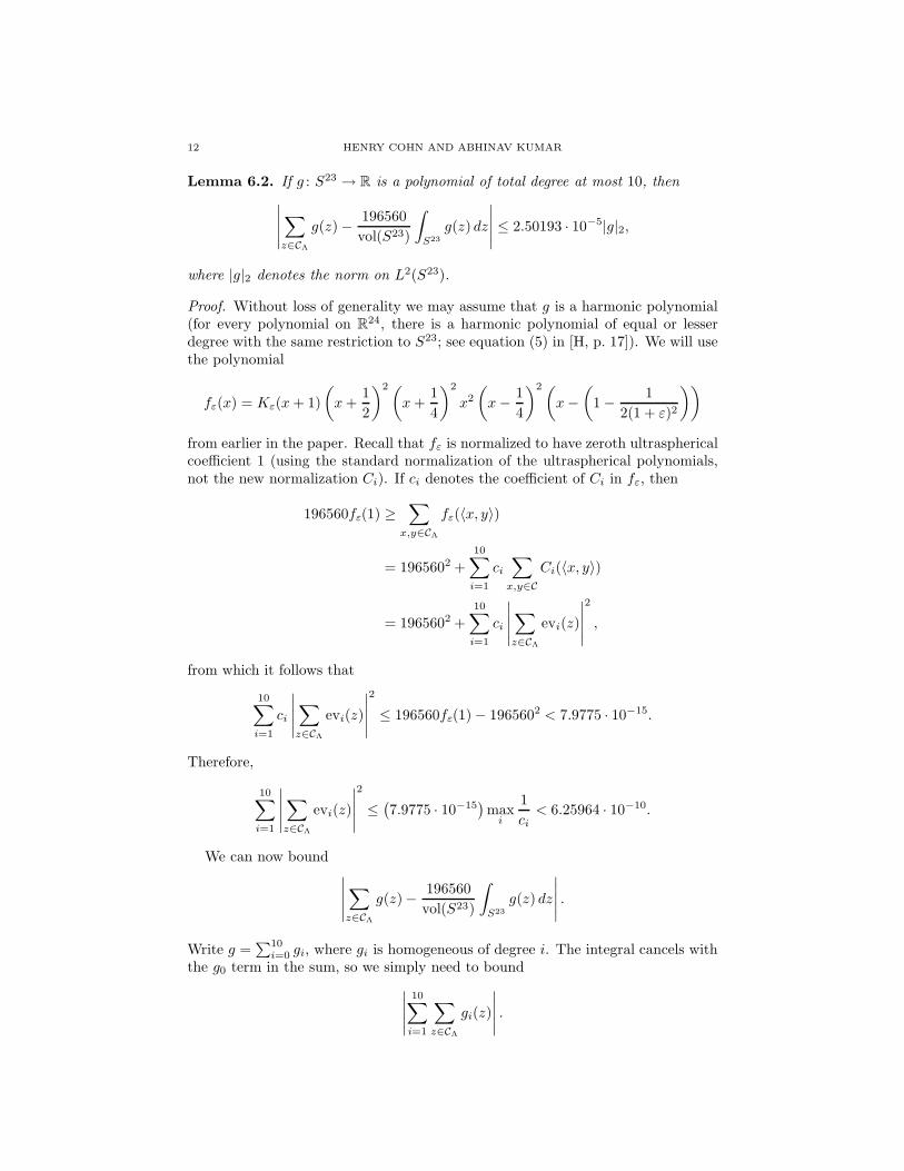
Lemma 6.2. If g : S23 → R is a polynomial of total degree at most 10, then
∣∣∣∣∣∑
z∈CΛ
g(z) − 196560
vol(S23)
∫
S23
g(z) dz
∣∣∣∣∣ ≤ 2.50193 · 10−5|g|2,
where |g|2 denotes the norm on L2(S23).
Proof. Without loss of generality we may assume that g is a harmonic polynomial(for every polynomial on R
24, there is a harmonic polynomial of equal or lesserdegree with the same restriction to S23; see equation (5) in [H, p. 17]). We will usethe polynomial
fε(x) = Kε(x + 1)
(x +
1
2
)2(x +
1
4
)2
x2
(x − 1
4
)2(x −
(1 − 1
2(1 + ε)2
))
from earlier in the paper. Recall that fε is normalized to have zeroth ultrasphericalcoefficient 1 (using the standard normalization of the ultraspherical polynomials,not the new normalization Ci). If ci denotes the coefficient of Ci in fε, then
196560fε(1) ≥∑
x,y∈CΛ
fε(〈x, y〉)
= 1965602 +
10∑
i=1
ci
∑
x,y∈C
Ci(〈x, y〉)
= 1965602 +10∑
i=1
ci
∣∣∣∣∣∑
z∈CΛ
evi(z)
∣∣∣∣∣
2
,
from which it follows that
10∑
i=1
ci
∣∣∣∣∣∑
z∈CΛ
evi(z)
∣∣∣∣∣
2
≤ 196560fε(1) − 1965602 < 7.9775 · 10−15.
Therefore,
10∑
i=1
∣∣∣∣∣∑
z∈CΛ
evi(z)
∣∣∣∣∣
2
≤(7.9775 · 10−15
)max
i
1
ci< 6.25964 · 10−10.
We can now bound∣∣∣∣∣∑
z∈CΛ
g(z)− 196560
vol(S23)
∫
S23
g(z) dz
∣∣∣∣∣ .
Write g =∑10
i=0 gi, where gi is homogeneous of degree i. The integral cancels withthe g0 term in the sum, so we simply need to bound
∣∣∣∣∣
10∑
i=1
∑
z∈CΛ
gi(z)
∣∣∣∣∣ .

OPTIMALITY AND UNIQUENESS OF THE LEECH LATTICE AMONG LATTICES 13
For that, we use the definition of the norm and the Cauchy-Schwarz inequality todeduce that
∣∣∣∣∣
10∑
i=1
∑
z∈CΛ
gi(z)
∣∣∣∣∣ ≤10∑
i=1
∣∣∣∣∣∑
z∈CΛ
evi(z)
∣∣∣∣∣ |gi|2
≤
√√√√10∑
i=1
∣∣∣∣∣∑
z∈CΛ
evi(z)
∣∣∣∣∣
2√√√√
10∑
i=1
|gi|22
≤ 2.50193 · 10−5|g|2,as desired. �
In fact, it follows immediately that CΛ is nearly a spherical 11-design in the samesense, because it is antipodal (if x ∈ CΛ then −x ∈ CΛ) and thus every homogeneouspolynomial of odd degree averages to 0 over CΛ. However, we will not need thatfact.
It is worth pointing out for completeness that the minimal vectors in Λ24 do notform a spherical 12-design: if y is a minimal vector then the polynomial
(16 − 〈x, y〉2
) (4 − 〈x, y〉2
)2 (1 − 〈x, y〉2
)2 〈x, y〉2
in x vanishes at each minimal vector but does not average to 0 over the sphere ofradius 2, because it is nonnegative on that sphere.
The constant 2.50193 · 10−5 in Lemma 6.2 can be made somewhat smaller forpolynomials of total degree at most 8 (using the same proof), and that is the onlycase we need later. However, the present bound suffices.
6.2. Intersection numbers. We will now use the fact that CΛ is nearly a spherical10-design to determine the intersection numbers (still following the techniques of[DGS]). As a computational aid, it is useful to know the following formula foraveraging homogeneous polynomials over the sphere:
1
vol(S23)
∫
S23
g(z) dz =
∫R24 g(z)e−|z|2 dz∫∞
0 rdeg ge−r2 vol(S23)r23 dr.
In the exact case of Λ24, we can compute the intersection numbers as follows.For each x, y ∈ C24 (the spherical code derived from the minimal vectors) with aspecified inner product, we need to determine the number of z ∈ C24 with specifiedinner products with x and y. Let Pγ(α, β) denote this number when 〈x, y〉 = γ,〈x, z〉 = α, and 〈y, z〉 = β. The cases γ = ±1 simply amount to the valencies, whichare determined automatically once the other intersection numbers are determined.For instance P1(α, β) = 0 unless α = β, and P1(α, α) =
∑β P0(α, β) once we
demonstrate that there every vector in C24 has a vector in C24 orthogonal to it(which follows from, say, showing that Pα(0, 0) 6= 0 for each α 6= ±1). Hence wewill focus on the remaining cases, i.e., γ 6= ±1.
For such a pair (x, y) with 〈x, y〉 = γ, a priori there are 49 unknowns Pγ(α, β)for α, β ∈ {−1,−1/2,−1/4, 0, 1/4, 1/2, 1}. We first note that Pγ(1, α) = Pγ(α, 1) =δα,γ , where δ is the Kronecker delta. Similarly Pγ(−1, α) = Pγ(α,−1) = δγ,−α.Thus we can eliminate ±1 from consideration, which reduces the problem to findingonly 25 unknowns. We will find 25 linear equations that determine these values.

14 HENRY COHN AND ABHINAV KUMAR
P0(0, 0) = 43164 P0(0, 1/2) = 2464 P0(0, 1/4) = 22528P0(1/2, 1/2) = 44 P0(1/2, 1/4) = 1024 P0(1/4, 1/4) = 11264
P1/2(0, 0) = 49896 P1/2(0, 1/2) = 891 P1/2(0, 1/4) = 20736P1/2(1/2, 1/2) = 891 P1/2(1/2,−1/2) = 1 P1/2(1/2, 1/4) = 2816P1/2(1/2,−1/4) = 0 P1/2(1/4, 1/4) = 20736 P1/2(1/4,−1/4) = 2816
P1/4(0, 0) = 44550 P1/4(0, 1/2) = 2025 P1/4(0, 1/4) = 22275P1/4(1/2, 1/2) = 275 P1/4(1/2,−1/2) = 0 P1/4(1/2, 1/4) = 2025P1/4(1/2,−1/4) = 275 P1/4(1/4, 1/4) = 15400 P1/4(1/4,−1/4) = 7128
Table 1. Intersection numbers for the Leech lattice minimal vectors.
Consider the polynomials gi,j(z) = 〈z, x〉i〈z, y〉j for i, j ∈ {0, 1, . . . , 4}. Let S bethe set {−1,−1/2,−1/4, 0, 1/4, 1/2, 1}. We then know that
∑
α,β∈S
αiβjPγ(α, β) =196560
vol(S23)
∫
S23
gi,j(z) dz,
because C24 is a spherical 11-design (although even an 8-design would suffice).These equations can be solved to yield the unknown values of Pγ(α, β). Note thatthe right hand side does not depend on the choice of x and y, only on γ = 〈x, y〉.Therefore we see that the solutions of these equations, which are the intersectionnumbers, are independent of x, y and only depend on γ. We solve one such systemof equations for each value of γ, and the values of the intersection numbers aretabulated in Table 1, which is a complete list modulo the symmetries
Pγ(α, β) = Pγ(β, α) = Pγ(−α,−β) = P−γ(α,−β).
(These numbers are of course known, but they are not tabulated in standard refer-ences such as [CS2], so we record them here for convenience.)
What happens when we are not necessarily dealing with exactly Λ24, but ratherwith Λ? Suppose we have x, y ∈ CΛ and we want to determine the number of
z ∈ CΛ with specified approximate inner products with them. Let Pγ(α, β) denotethe intersection numbers for CΛ (which may depend on x and y); here we use α,β, and γ to denote exact elements of {0,±1/4,±1/2,±1}, and the inner productsfrom CΛ are required to be approximately equal to them. Then we have
∑
α,β∈S
αiβjPγ(α, β) =∑
w∈CΛ,〈w,x〉≈α,〈w,y〉≈β
αiβj
≈∑
w∈CΛ
〈w, x〉i〈w, y〉j
=∑
w∈CΛ
gi,j(w)
≈ 196560
vol(S23)
∫
S23
gi,j(z) dz
≈ 196560
vol(S23)Gi,j(γ),

OPTIMALITY AND UNIQUENESS OF THE LEECH LATTICE AMONG LATTICES 15
where
Gi,j(γ) =
∫
S23
〈z, u〉i〈z, v〉j dz
with 〈u, v〉 = γ (recall that 〈x, y〉 ≈ γ).If these approximations are close enough, we should get about the same values
for Pγ(α, β) as we did for Pγ(α, β), and this will show that the intersection numbersmust be the same.
Lemma 6.3. Let α, β ∈ {0,±1/4,±1/2,±1} and a, b ∈ [−(1/2+σ), 1/2+σ]∪{±1}with max{|a − α|, |b − β|} ≤ σ < 0.1. Then for i, j ≥ 0,
|aibj − αiβj | ≤ (1 + 2σ)σ.
Proof. We begin by bounding |αi − ai|. For i = 0 or α ∈ {±1}, αi = ai, so we canassume that i > 0 and α ∈ {0,±1/4,±1/2}. Then
αi − ai = (α − a)
i−1∑
k=0
αkai−1−k.
If we apply the triangle inequality (together with |α−a| ≤ σ and |α|, |a| ≤ 1/2+σ),we find that
(6.1) |αi − ai| ≤ i(1/2 + σ)i−1σ.
The function n(1/2 + σ)n−1 on nonnegative integers attains its maximum valuewhen n = 2, from which it follows that |αi − ai| ≤ (1 + 2σ)σ. Note that this is thespecial case of the lemma in which β = b = ±1. Thus, we can henceforth assumethat neither β nor b is ±1, and by symmetry we can assume the same for α and a.
For the general case, we notice that
αiβj − aibj = (αi − ai)βj + ai(βj − bj),
so
|αiβj − aibj | ≤ |αi − ai| · |βj | + |ai| · |βj − bj|.It now follows from (6.1) that
|αiβj − aibj| ≤ (i + j)(1/2 + σ)i+j−1σ.
The right hand side is at most (1 + 2σ)σ, as before. �
Now we need to make precise the errors in all three approximations in∑
α,β∈S
αiβj Pγ(α, β) ≈∑
w∈CΛ
gi,j(w)
≈ 196560
vol(S23)
∫
S23
gi,j(z) dz
≈ 196560
vol(S23)Gi,j(γ).
The first follows from Lemma 6.3:∣∣∣∣∣∣
∑
α,β∈S
αiβjPγ(α, β) −∑
w∈CΛ
gi,j(w)
∣∣∣∣∣∣≤∑
w∈CΛ
(1 + 2σ)σ = 196560(1 + 2σ)σ,
because |αiβj − aibj | ≤ (1 + 2σ)σ for 〈w, x〉 = a ≈ α and 〈w, y〉 = b ≈ β.

16 HENRY COHN AND ABHINAV KUMAR
The second we have already estimated sufficiently well in Lemma 6.2, in termsof |gi,j |2. Because |gi,j(z)| ≤ 1 for all z, we have
|gi,j |2 ≤√
vol(S23) =
√24 · π12
12!=
π6
√19958400
.
It follows that∣∣∣∣∣∑
w∈CΛ
gi,j(w) − 196560
vol(S23)
∫
S23
gi,j(z) dz
∣∣∣∣∣ ≤π6
√19958400
·2.50193·10−5 < 5.3841·10−6.
Finally, one can check by straightforward computation of each case that if 〈x, y〉differs from one of −1/2,−1/4, 0, 1/4, 1/2 by at most σ (where 0 ≤ σ ≤ 1), and0 ≤ i, j ≤ 4, then
196560
vol(S23)
∫
S23
gi,j(z) dz
differs by at most 8190σ from what it would be if σ were zero. (In fact, if oneexpands this quantity as a power series in σ, then the sum of the absolute valuesof the coefficients is at most 8190.) Therefore the error in the last approximationis at most 8190σ.
Thus ∑
α,β∈S
αiβjPγ(α, β) =196560
vol(S23)Gi,j(γ) + Di,j ,
where
|Di,j | < 196560(1 + 2σ)σ + 8190σ + 5.3841 · 10−6 < 6.7023 · 10−6.
As before the values of Pγ(±1, α) and Pγ(α,±1) are known and are the same asthe corresponding Pγ(±1, α) and Pγ(α,±1). Thus they serve as constants in theequation and do not contribute to the error.
Let A be the matrix of coefficients for these equations. One can check that|A−1|∞ = 7225. (Here, | · |∞ denotes the ∞-norm on matrices, which is induced bythe ℓ∞ norm on vectors. It is the maximum over all rows of the sum of the absolutevalues of the elements in that row.) It follows that the intersection numbers in CΛ
differ by at most
7225 · 6.7023 · 10−6 < 0.05
from those in C24. Because they must be integers, this proves that they are thesame as in C24 (in particular, they do not depend on the choice of x and y, althoughwhat we have proved is far stronger).
The computer file verifyrest.txt carries out all these calculations (as well asthose from several other points in this paper). In it, we assume without loss of
generality that γ > 0 because Pγ(α, β) = P−γ(α,−β).
6.3. Uniqueness of association scheme. The spherical code C24 determines a 6-class association scheme A24 if we partition elements (x, y) of C24 ×C24 with x 6= yaccording to their inner products 〈x, y〉. We can similarly form the associationscheme AΛ of the spherical code CΛ coming from Λ, where this time we groupelements according to their approximate inner products. We wish to show thatthese two association schemes are isomorphic. We will need to know that this6-class association scheme A24 is uniquely determined by its size, valencies, andintersection numbers. That can be proved as follows.

OPTIMALITY AND UNIQUENESS OF THE LEECH LATTICE AMONG LATTICES 17
Let N = 196560, let C = 6/N = 1/32760, and let u1, . . . , uN be the minimalvectors of the Leech lattice. The following lemma restates the (known) fact thatΛ24 is strongly eutactic. We provide a proof here to make this article more self-contained.
Lemma 6.4. For every x ∈ R24,
〈x, x〉 = C
N∑
i=1
〈x, ui〉2.
Proof. Because the minimal vectors of Λ24 form a spherical 2-design, the polynomialy 7→ 〈x, y〉2 has the same average over {u1, . . . , uN} and the sphere of radius 2 inR
24, which is 4 times the average over the unit sphere. To average over the unitsphere, it will be convenient to work with orthonormal bases of R
24. For eachorthonormal basis e1, . . . , e24, we have |x|2 =
∑i〈x, ei〉2. If we average over all
orthonormal bases, then each of e1, . . . , e24 is uniformly distributed over the unitsphere, and therefore the average of y 7→ 〈x, y〉2 over the unit sphere is |x|2/24. Itfollows that the average over the sphere of radius 2 is |x|2/6, so
1
N
N∑
i=1
〈x, ui〉2 = |x|2/6,
as desired. �
Theorem 6.5. There is only one 6-class association scheme with the same size,
valencies and intersection numbers as the association scheme of minimal vectors of
the Leech lattice.
Proof. Let A = {ai : 1 ≤ i ≤ 196560} be such an association scheme, with A2
partitioned into classes as
A2 = A1 ∪ A1/2 ∪ A1/4 ∪ A0 ∪ A−1/4 ∪ A−1/2 ∪ A−1
(labeled according to the corresponding inner products in the Leech case, when theminimal vectors are rescaled to lie on the unit sphere).
Let A1, A1/2, . . . , A−1 denote the adjacency matrices of the identity relation andthe six classes; in other words,
(Aα)i,j =
{1 if (ai, aj) ∈ Aα, and
0 otherwise.
These matrices are symmetric and commute with each other. Their span formsan algebra, called the Bose-Mesner algebra, whose product is determined by thevalencies and intersection numbers. (See [BH, p. 755].) Namely,
AαAβ =∑
γ
Pγ(α, β)Aγ .
Furthermore, note that because the Aα’s have only 0 or 1 as entries, are not identi-cally zero, and sum to the all 1’s matrix, they must be linearly independent. Thus,the Bose-Mesner algebra is completely determined by the valencies and intersectionnumbers, with no additional relations possible.
Let
P = 4C
(A1 +
1
2A1/2 +
1
4A1/4 −
1
4A−1/4 −
1
2A−1/2 − A−1
).

18 HENRY COHN AND ABHINAV KUMAR
If the association scheme A comes from the Leech lattice, then P is C times theGram matrix of the 196560 minimal vectors (not rescaled to the unit sphere). Weclaim that P is a projection matrix, i.e., P 2 = P . One way to check that is to usethe valencies and intersection numbers to compute P 2 and verify that it equals P .That is somewhat cumbersome to check by hand, so we will instead give a longerbut conceptually simpler proof.
First, we check it in the case of the actual Leech lattice association scheme, usingLemma 6.4. From
〈x, x〉 = C
N∑
i=1
〈x, ui〉2
it follows that
〈x, y〉 =1
2(〈x + y, x + y〉 − 〈x, x〉 − 〈y, y〉)
=C
2
N∑
i=1
(〈x + y, ui〉2 − 〈x, ui〉2 − 〈y, ui〉2
)
= C
N∑
i=1
〈x, ui〉〈y, ui〉.
Therefore the (i, j) entry of P 2 is
(P 2)i,j = C2N∑
k=1
〈ui, uk〉〈uj , uk〉 = C〈ui, uj〉 = Pi,j ,
so for the Leech lattice P is a projection matrix. Because the structure of the Bose-Mesner algebra is completely determined by the valencies and intersection numbers,the same must always be true.
Thus, P is always a projection matrix (in fact, an orthogonal projection becauseP is symmetric). The trace of P is 4C times the trace of A1, because no other Aα’shave entries on the diagonal. The trace is therefore 4NC = 24, so P projects ontoa 24-dimensional subspace.
Consider the images of the N = 196560 unit vectors (namely e1, . . . , e196560)under P . Their inner products are simply the entries of P , since 〈Pei, P ej〉 =
〈ei, P2ej〉 = 〈ei, P ej〉 = Pi,j , and if one rescales the vectors by 1/
√4C so that
they lie on the unit sphere, then the result is a 196560-point kissing configurationin R
24. (Appendix B reviews the kissing problem.) The only such configurationis the kissing configuration of the Leech lattice (see [BS], which was reprinted asChapter 14 of [CS2]), up to orthogonal transformations of R
24. Thus, P/C mustbe the Gram matrix of the minimal vectors in the Leech lattice.
It follows that A is isomorphic to A24 (in particular, ai 7→ P (ei)/√
4C yieldsan isomorphism). Thus, A24 is determined by its size and intersection numbers, asdesired. �
7. Inner product bounds
We will first use the intersection numbers and isomorphism of association schemesto prove better bounds on σ. We already know that for all nearly minimal vectorsu,
4 ≤ 〈u, u〉 ≤ 4(1 + ε)2 < 4 + 9ε.
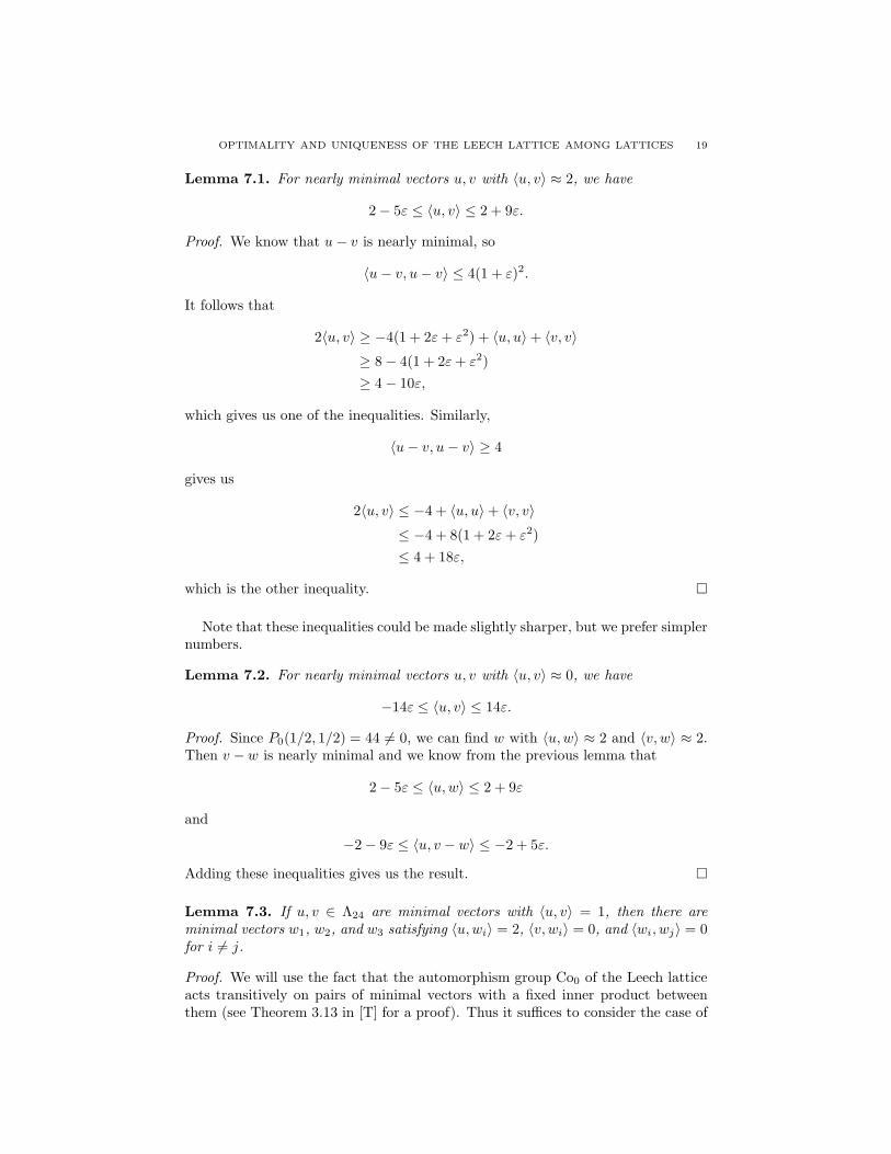
OPTIMALITY AND UNIQUENESS OF THE LEECH LATTICE AMONG LATTICES 19
Lemma 7.1. For nearly minimal vectors u, v with 〈u, v〉 ≈ 2, we have
2 − 5ε ≤ 〈u, v〉 ≤ 2 + 9ε.
Proof. We know that u − v is nearly minimal, so
〈u − v, u − v〉 ≤ 4(1 + ε)2.
It follows that
2〈u, v〉 ≥ −4(1 + 2ε + ε2) + 〈u, u〉 + 〈v, v〉≥ 8 − 4(1 + 2ε + ε2)
≥ 4 − 10ε,
which gives us one of the inequalities. Similarly,
〈u − v, u − v〉 ≥ 4
gives us
2〈u, v〉 ≤ −4 + 〈u, u〉 + 〈v, v〉≤ −4 + 8(1 + 2ε + ε2)
≤ 4 + 18ε,
which is the other inequality. �
Note that these inequalities could be made slightly sharper, but we prefer simplernumbers.
Lemma 7.2. For nearly minimal vectors u, v with 〈u, v〉 ≈ 0, we have
−14ε ≤ 〈u, v〉 ≤ 14ε.
Proof. Since P0(1/2, 1/2) = 44 6= 0, we can find w with 〈u, w〉 ≈ 2 and 〈v, w〉 ≈ 2.Then v − w is nearly minimal and we know from the previous lemma that
2 − 5ε ≤ 〈u, w〉 ≤ 2 + 9ε
and
−2 − 9ε ≤ 〈u, v − w〉 ≤ −2 + 5ε.
Adding these inequalities gives us the result. �
Lemma 7.3. If u, v ∈ Λ24 are minimal vectors with 〈u, v〉 = 1, then there are
minimal vectors w1, w2, and w3 satisfying 〈u, wi〉 = 2, 〈v, wi〉 = 0, and 〈wi, wj〉 = 0for i 6= j.
Proof. We will use the fact that the automorphism group Co0 of the Leech latticeacts transitively on pairs of minimal vectors with a fixed inner product betweenthem (see Theorem 3.13 in [T] for a proof). Thus it suffices to consider the case of

20 HENRY COHN AND ABHINAV KUMAR
a particular pair (u, v) of minimal vectors with inner product 1. Let
u =1√8(1, 1, . . . , 1, 1,−3),
v =1√8(0, 0, . . . , 0,−4,−4),
w1 =1√8(2, 2, 2, 2, 2, 2, 2, 2, 0, 0, . . . , 0),
w2 =1√8(0, 0, . . . , 0, 4,−4), and
w3 =1√8(0, 0, 0, 0, 0, 0, 0, 0, 2, 2, 0, 0, 2, 2, 0, 0, 2, 2, 0, 0, 2, 2, 0, 0).
(see [CS2, p. 131] for a description of the minimal vectors). It is easily checked thatthe inner products are as desired. �
Lemma 7.4. For nearly minimal vectors u, v with 〈u, v〉 ≈ 1, we have
1 − 72ε ≤ 〈u, v〉 ≤ 1 + 75ε.
Proof. We know that the association schemes of the Leech lattice Λ24 and ourgiven lattice Λ are the same. Let u′, v′ be the corresponding vectors in the Leechlattice (corresponding via some fixed isomorphism of association schemes). Since〈u′, v′〉 = 1, we know that we can find w′
1, w′2, and w′
3 in the Leech lattice satisfying〈u′, w′
i〉 = 2, 〈v′, w′i〉 = 0, and 〈w′
i, w′j〉 = 0 by Lemma 7.3. Let w1, w2, w3 be
the corresponding vectors in Λ. Then the relations 〈u, wi〉 ≈ 2, 〈v, wi〉 ≈ 0, and〈wi, wj〉 ≈ 0 must hold in Λ. It follows by a short computation that 2u− v −w1 −w2 − w3 is a nearly minimal vector. Therefore
4 ≤ 〈2u − v − w1 − w2 − w3, 2u − v − w1 − w2 − w3〉= 4〈u, u〉 + 〈v, v〉 +
∑
i
〈wi, wi〉 − 4〈u, v〉
− 4∑
i
〈u, wi〉 + 2∑
i
〈v, wi〉 + 2∑
i<j
〈wi, wj〉.
It follows that
4〈u, v〉 ≤ −4 + 4〈u, u〉 + 〈v, v〉 +∑
i
〈wi, wi〉
− 4∑
i
〈u, wi〉 + 2∑
i
〈v, wi〉 + 2∑
i<j
〈wi, wj〉
≤ −4 + 8(4 + 9ε) − 12(2 − 5ε) + 12(14ε).
Thus, 〈u, v〉 ≤ 1 + 75ε. Similarly,
4 + 9ε ≥ 〈2u − v − w1 − w2 − w3, 2u − v − w1 − w2 − w3〉= 4〈u, u〉 + 〈v, v〉 +
∑
i
〈wi, wi〉 − 4〈u, v〉
− 4∑
i
〈u, wi〉 + 2∑
i
〈v, wi〉 + 2∑
i<j
〈wi, wj〉.

OPTIMALITY AND UNIQUENESS OF THE LEECH LATTICE AMONG LATTICES 21
It follows that
4〈u, v〉 ≥ −4 − 9ε + 4〈u, u〉+ 〈v, v〉 +∑
i
〈wi, wi〉
− 4∑
i
〈u, wi〉 + 2∑
i
〈v, wi〉 + 2∑
i<j
〈wi, wj〉
≥ −4 − 9ε + 8(4) − 12(2 + 9ε) + 12(−14ε).
Thus, 〈u, v〉 ≥ 1 − (285/4)ε ≥ 1 − 72ε. �
We have proved the following proposition.
Proposition 7.5. If u, v ∈ Λ are nearly minimal vectors, then 〈u, v〉 differs from
an element of {0,±1,±2,±4} by at most 75ε.
8. A basis of nearly minimal vectors
We wish to prove that Λ must have a basis of nearly minimal vectors. We firstprove that the nearly minimal vectors span Λ. Let x ∈ Λ be as small a vectoras possible without being in the span of the nearly minimal vectors. Then theredoes not exist a nearly minimal vector u such that |u − x| < |x|. We know that
|x| >√
6(1 − µ) and 2 ≤ |u| ≤ 2(1 + ε) for each nearly minimal u. Because|u − x| ≥ |x|, we have
〈u, x〉 ≤ |u|2/2 ≤ 2(1 + ε)2.
Consider the unit vectors x/|x| and u/|u|. We have⟨
u
|u| ,x
|x|
⟩≤ 2(1 + ε)2√
6(1 − µ) · 2<
1
2.
If we extend the spherical code CΛ of vectors of the form u/|u| to CΛ∪{x/|x|}, thenit will contain 196561 vectors without changing the minimal angle, and we haveseen that that is impossible. Thus, the nearly minimal vectors do span the lattice.
The same argument (with ε = µ = 0) also proves the following fact: if the kissingconfiguration of a lattice is an optimal kissing configuration for its dimension, thenthe lattice is spanned by its minimal vectors.
Now let B be 1/√
8 times the matrix
4 −4 0 0 0 0 0 0 0 0 0 0 0 0 0 0 0 0 0 0 0 0 0 0
4 4 0 0 0 0 0 0 0 0 0 0 0 0 0 0 0 0 0 0 0 0 0 0
4 0 4 0 0 0 0 0 0 0 0 0 0 0 0 0 0 0 0 0 0 0 0 0
4 0 0 4 0 0 0 0 0 0 0 0 0 0 0 0 0 0 0 0 0 0 0 0
4 0 0 0 4 0 0 0 0 0 0 0 0 0 0 0 0 0 0 0 0 0 0 0
4 0 0 0 0 4 0 0 0 0 0 0 0 0 0 0 0 0 0 0 0 0 0 0
4 0 0 0 0 0 4 0 0 0 0 0 0 0 0 0 0 0 0 0 0 0 0 0
2 2 2 2 2 2 2 2 0 0 0 0 0 0 0 0 0 0 0 0 0 0 0 0
4 0 0 0 0 0 0 0 4 0 0 0 0 0 0 0 0 0 0 0 0 0 0 0
4 0 0 0 0 0 0 0 0 4 0 0 0 0 0 0 0 0 0 0 0 0 0 0
4 0 0 0 0 0 0 0 0 0 4 0 0 0 0 0 0 0 0 0 0 0 0 0
2 2 2 2 0 0 0 0 2 2 2 2 0 0 0 0 0 0 0 0 0 0 0 0
4 0 0 0 0 0 0 0 0 0 0 0 4 0 0 0 0 0 0 0 0 0 0 0
2 2 0 0 2 2 0 0 2 2 0 0 2 2 0 0 0 0 0 0 0 0 0 0
2 0 2 0 2 0 2 0 2 0 2 0 2 0 2 0 0 0 0 0 0 0 0 0
2 0 0 2 2 0 0 2 2 0 0 2 2 0 0 2 0 0 0 0 0 0 0 0
4 0 0 0 0 0 0 0 0 0 0 0 0 0 0 0 4 0 0 0 0 0 0 0
2 0 2 0 2 0 0 2 2 2 0 0 0 0 0 0 2 2 0 0 0 0 0 0
2 0 0 2 2 2 0 0 2 0 2 0 0 0 0 0 2 0 2 0 0 0 0 0
2 2 0 0 2 0 2 0 2 0 0 2 0 0 0 0 2 0 0 2 0 0 0 0
0 2 2 2 2 0 0 0 2 0 0 0 2 0 0 0 2 0 0 0 2 0 0 0
0 0 0 0 0 0 0 0 2 2 0 0 2 2 0 0 2 2 0 0 2 2 0 0
0 0 0 0 0 0 0 0 2 0 2 0 2 0 2 0 2 0 2 0 2 0 2 0
−3 1 1 1 1 1 1 1 1 1 1 1 1 1 1 1 1 1 1 1 1 1 1 1
.

22 HENRY COHN AND ABHINAV KUMAR
The rows of B form a basis of Λ24 consisting of minimal vectors (see Figure 4.12in [CS2]). One can compute the inverse matrix and check that its entries are
integers divided by√
8. The largest entry of B−1, in absolute value, is −13/√
8, so
|B−1|∞ ≤ 24 · 13/√
8.Let u′
1, . . . , u′24 be the rows of B. Every minimal vector u′ is a linear combination∑
i ciu′i of this basis, and the coefficients are bounded by
|ci| ≤ |B−1|∞|u′|∞ ≤ (24 · 13/√
8) · (4/√
8) = 156.
Consider the corresponding nearly minimal vectors u1, . . . , u24 of Λ (under an iso-morphism of association schemes). We next prove that they form a basis.
We need only check that u1, . . . , u24 span the nearly minimal vectors of Λ. Ifu is any nearly minimal vector, the isomorphism of association schemes gives usnumbers c1, . . . , c24 such that u should be
∑i ciui (i.e., the corresponding equality
is true for the Leech lattice). We first check that∑
i ciui is a nearly minimal vector,and then that it equals u. To check that it is nearly minimal, we just need to knowthat all inner products of nearly minimal vectors are within 75ε of what they are inthe Leech lattice (Proposition 7.5). When we compute the norm of
∑i ciui, each
inner product 〈ui, uj〉 could be off by as much as 75ε, and multiplied by up to 1562.There are 242 such pairs, for a total error of at most 1562 ·242 ·75ε = 1051315200ε,which is minuscule (less than 10−17). Because the next smallest vectors beyond the
nearly minimal vectors have norms at least√
6(1 − µ), we conclude that∑
i ciui
must be nearly minimal.To check that u =
∑i ciui, we need only compute their inner product and verify
that it is approximately 4. This time, the maximum error is 24 · 156 · 75ε, which isagain small enough by a huge margin.
Thus, u1, . . . , u24 form a basis of Λ, and their inner products are all within 75εof what they would be in the Leech lattice.
9. Local optimality of Λ24
In this section, we will prove in detail that the Leech lattice is locally optimal,and provide quantitative bounds. We will follow the notation and techniques from[GL] closely. The basic result is Voronoi’s theorem, which says that a lattice is alocal maximum for sphere packing density if and only if it is perfect and eutactic.In this section of the paper only, Λ will denote an arbitrary lattice in R
n.It is convenient to work in terms of the quadratic form Q associated to Λ. Choose
a lattice basis {bi}, and for a vector x ∈ Rn (with coordinates x1, . . . , xn) define
Q(x) =
⟨n∑
i=1
xibi,
n∑
i=1
xibi
⟩.
The matrix of Q is S = (si,j)ni,j=1, where si,j = 〈bi, bj〉.
Let M denote the minimal nonzero norm of Λ, and let u1, . . . , uN ∈ Zn be the
coefficient vectors of the minimal vectors in terms of the basis {bi}. Thus, for1 ≤ i ≤ N ,
Q(ui) = M.
Recall that Q is perfect if these equations completely determine the quadratic formQ. Equivalently, every quadratic form that vanishes at u1, . . . , uN must vanisheverywhere.

OPTIMALITY AND UNIQUENESS OF THE LEECH LATTICE AMONG LATTICES 23
Let D denote the determinant of S, and let S = (si,j)ni,j=1 denote the adjoint
matrix, where
si,j =∂D
∂si,j.
Strictly speaking this is an abuse of notation, but of course it means we take thepartial derivatives of D as if the entries of S were variables, and then substitutetheir actual values.
In other words, SS is D times the identity matrix. (It might seem that a trans-
pose is missing, but note that all our matrices are symmetric.) Let Q be the
quadratic form with matrix S. Then Λ is eutactic if there are positive numbersd1, . . . , dN such that for all x ∈ R
n,
Q(x) =
N∑
k=1
dk〈uk, x〉2.
It is known that Λ24 is perfect and eutactic, with d1 = · · · = d196560 = 1/32760.For completeness we sketch a proof. Lemma 6.4 proves that the Leech lattice iseutactic.
Lemma 9.1. The Leech lattice Λ24 is perfect.
Proof. Suppose Q is a quadratic form that vanishes on the minimal vectors. Thenthe symmetric bilinear form B corresponding to Q satisfies B(ui, ui) = 0. We firstshow that B(u, v) = 0 for all minimal vectors u, v. If 〈u, v〉 = 2 we use the fact thatu − v is minimal to see that
B(u, v) =1
2(B(u, u) + B(v, v) − B(u − v, u − v)) = 0.
If 〈u, v〉 = 0, then since P0(1/2,−1/2) = 44 6= 0, we can find w with 〈u, w〉 = 2 and〈v, w〉 = −2. Then v + w is nearly minimal and we know
0 = B(u, w) = B(u, v + w);
subtracting these two gives us the result. If 〈u, v〉 = 1, then by Lemma 7.3 thereare minimal vectors w1, w2, and w3 with 〈u, wi〉 = 2, 〈v, wi〉 = 0, and 〈wi, wj〉 = 0for i 6= j. It follows that 2u − v − w1 − w2 − w3 is a minimal vector. Therefore
0 = B(2u − v − w1 − w2 − w3, 2u − v − w1 − w2 − w3)
= 4B(u, u) + B(v, v) +∑
i
B(wi, wi) − 4B(u, v)
− 4∑
i
B(u, wi) + 2∑
i
B(v, wi) + 2∑
i<j
B(wi, wj)
= −4B(u, v) + 0.
This forces B(u, v) = 0. Finally, the result for 〈u, v〉 < 0 follows from the above bynoticing B(u, v) = −B(u,−v) and 〈u,−v〉 > 0.
To conclude the proof, we use the above information on a basis of minimal vectorsto see that B, and hence Q, is identically zero. �
We begin by proving one direction of Voronoi’s theorem. This proof is the onegiven in [GL, §39], where one can also find a proof of the converse. We give thedetails of this direction because we will need to examine it in detail to derivequantitative estimates, and because it is the only direction we will need.

24 HENRY COHN AND ABHINAV KUMAR
Theorem 9.2 (Voronoi [Vo]). If Λ is perfect and eutactic, then it is a strict local
maximum for density.
Proof. We wish to show that if Λ is perturbed slightly (other than simply by scalingand isometries), then D−1/nM must strictly decrease. We perturb S = (si,j) bychanging it to (si,j + ρti,j), where tj,i = ti,j and ρ > 0 is small. We assume (ti,j)is not identically zero. Let Qρ denote the corresponding quadratic form, and letDρ be the determinant of the matrix (si,j + ρti,j). We will show that for any fixedmatrix (ti,j) not proportional to S, if ρ is sufficiently small, then there exists a ksuch that
D−1/nρ Qρ(uk) < D−1/nM.
Because Qρ(uk) is no smaller than the minimal norm of Qρ (i.e., the minimumvalue of Qρ on Z
n \ {0}), this inequality is what we want.First, note that without loss of generality we can assume that
(9.1)∑
i,j
si,jti,j = 0.
The reason is that ∑
i,j
si,jsi,j = nD 6= 0.
Every perturbation can be broken up into the sum of a perturbation proportional toS and a perturbation satisfying (9.1). If we deal with the latter, then we can ignorethe former (which rescales the lattice but does not change its packing density).
Thus, we assume (9.1) from now on. Then the determinant Dρ is given by
Dρ = det(si,j + ρti,j) = det(si,j) + ρ∑
i,j
ti,j si,j + O(ρ2)
= D + O(ρ2) as ρ → 0.
Because Λ is eutactic,
Q(x) =N∑
k=1
dk〈uk, x〉2
for all x ∈ Rn. The associated symmetric bilinear form is
N∑
k=1
dk〈uk, x〉〈uk, y〉,
from which it follows that
si,j =
N∑
k=1
dk(uk)i(uk)j ,
where (uk)i denotes the i-th coefficient of uk. Therefore
N∑
k=1
dk
∑
i,j
ti,j(uk)i(uk)j =∑
i,j
si,jti,j = 0.
Because Λ is perfect, the inner sum on the left hand side in the above equationcannot vanish for all k. Therefore, there exists a k for which it is negative, say
∑
i,j
ti,j(uk)i(uk)j ≤ −α

OPTIMALITY AND UNIQUENESS OF THE LEECH LATTICE AMONG LATTICES 25
with α > 0. Then
Qρ(uk) =∑
(si,j + ρti,j)(uk)i(uk)j ≤ M − ρα,
and hence
D−1/nρ Qρ(uk) ≤ D−1/nM(1 − ρα/M)(1 + O(ρ2))−1/n < D−1/nM
if ρ is positive and small enough. This proves that Λ is a strict local optimum fordensity when (si,j) is perturbed in the direction of (ti,j). In fact, the choices ofα and the implicit constant in the big-O can be made uniformly in (ti,j), given∑
i,j |ti,j |2 = 1. Thus Λ is a strict local optimum for density. �
We now compute numerical bounds on the perturbations. We use the same basisof Λ24 as before. The corresponding Gram matrix is
4 0 2 2 2 2 2 0 2 2 2 0 2 0 1 1 2 1 1 0 −1 0 0 −2
0 4 2 2 2 2 2 2 2 2 2 2 2 2 1 1 2 1 1 2 1 0 0 −1
2 2 4 2 2 2 2 2 2 2 2 2 2 1 2 1 2 2 1 1 1 0 0 −1
2 2 2 4 2 2 2 2 2 2 2 2 2 1 1 2 2 1 2 1 1 0 0 −1
2 2 2 2 4 2 2 2 2 2 2 1 2 2 2 2 2 2 2 2 1 0 0 −1
2 2 2 2 2 4 2 2 2 2 2 1 2 2 1 1 2 1 2 1 0 0 0 −1
2 2 2 2 2 2 4 2 2 2 2 1 2 1 2 1 2 1 1 2 0 0 0 −1
0 2 2 2 2 2 2 4 1 1 1 2 1 2 2 2 1 2 2 2 2 0 0 1
2 2 2 2 2 2 2 1 4 2 2 2 2 2 2 2 2 2 2 2 1 1 1 −1
2 2 2 2 2 2 2 1 2 4 2 2 2 2 1 1 2 2 1 1 0 1 0 −1
2 2 2 2 2 2 2 1 2 2 4 2 2 1 2 1 2 1 2 1 0 0 1 −1
0 2 2 2 1 1 1 2 2 2 2 4 1 2 2 2 1 2 2 2 2 1 1 1
2 2 2 2 2 2 2 1 2 2 2 1 4 2 2 2 2 1 1 1 1 1 1 −1
0 2 1 1 2 2 1 2 2 2 1 2 2 4 2 2 1 2 2 2 2 2 1 1
1 1 2 1 2 1 2 2 2 1 2 2 2 2 4 2 1 2 2 2 2 1 2 1
1 1 1 2 2 1 1 2 2 1 1 2 2 2 2 4 1 2 2 2 2 1 1 1
2 2 2 2 2 2 2 1 2 2 2 1 2 1 1 1 4 2 2 2 1 1 1 −1
1 1 2 1 2 1 1 2 2 2 1 2 1 2 2 2 2 4 2 2 2 2 1 1
1 1 1 2 2 2 1 2 2 1 2 2 1 2 2 2 2 2 4 2 2 1 2 1
0 2 1 1 2 1 2 2 2 1 1 2 1 2 2 2 2 2 2 4 2 1 1 1
−1 1 1 1 1 0 0 2 1 0 0 2 1 2 2 2 1 2 2 2 4 2 2 2
0 0 0 0 0 0 0 0 1 1 0 1 1 2 1 1 1 2 1 1 2 4 2 2
0 0 0 0 0 0 0 0 1 0 1 1 1 1 2 1 1 1 2 1 2 2 4 2
−2 −1 −1 −1 −1 −1 −1 1 −1 −1 −1 1 −1 1 1 1 −1 1 1 1 2 2 2 4
.
Suppose we assume that the Gram matrix entries are perturbed by ρti,j wheremax{|ti,j |} ≤ 1 (and (9.1) holds—we will eventually deal with the case where itdoes not). Then, using the same notation as in the proof of Theorem 9.2,
Dρ − D =∑
T
ρdim T det(T ) det(T ),
where T ranges over all nonvacuous minors of (ti,j) and det(T ) is the correspondingcofactor of the matrix S. (The D term corresponds to the case where T is vacuous,i.e., contains no rows or columns.) This expansion follows from combining theLaplace expansion (see [Mu, §95]) with multilinearity, and is known as Albeggiani’stheorem [Mu, §96].
Now let dimT = k. Then | det(T )| ≤ kk/2 by Hadamard’s inequality, since the
length of each row of T is at most√
k (see (7.8.2) in [HJ]). It follows that the
absolute value of the sum of ρk det(T ) det(T ) over k-dimensional T is bounded bykk/2ρkAk, where Ak is the sum of the absolute values of the (24 − k)-dimensional
minors of the Gram matrix. For k ≥ 3 we use the simple bound Ak ≤(24k
)2 · (42 +
(24−k−1)(22))(24−k)/2 (the first factor is the number of (24−k)× (24−k) minors,and the second is the above bound on the determinant of the cofactor, using thefact that the largest entry in each row of S is 4 and the other entries are at most2 in absolute value). For k = 2 we explicitly compute the sum of absolute values

26 HENRY COHN AND ABHINAV KUMAR
of the 22 × 22 minors, and find that it is 818153. Putting all this together, we seethat for 0 < ρ < 10−20,
(9.2) Dρ ≥ 1 − ρ2(22/2 · 818153 + 2 · 108
),
where the 2 · 108 term bounds the contribution from all higher powers of ρ. (Recallthat D = 1 for the Leech lattice.) See the computer file verifygram.txt for thedetails of this calculation.
Next, we find an α that works for any choice of ti,j such that max{|ti,j |} = 1.This is done by linear programming as follows.
We find an α > 0 such that for all (i0, j0), and for all ti,j subject to the constraints−1 ≤ ti,j ≤ 1 for (i, j) 6= (i0, j0), ti,j = tj,i, ti0,j0 = 1, and
∑i,j si,jti,j = 0, the
following inequality holds for some minimal vector uk:∑
i,j
ti,j(uk)i(uk)j ≤ −α.
We do the same for ti0,j0 = −1. All these linear programs can be solved by com-puter, and it appears that α = 1/23 works and is the largest possible value of α.However, that is the result of floating point calculations that are not rigorous. Wewill be content with proving (without computer assistance) that α = 4/1055 satis-fies these properties. This weaker bound will suffice for our purposes and is provedin Section 10.
We conclude that for every perturbation by ti,j where max{|ti,j |} = ρ and∑i,j si,jti,j = 0, there exists a k such that for 0 < ρ < 10−20,
(9.3)D
−1/24ρ Qρ(uk)
D−1/24 · M ≤ (1 − ρ/1055)(1− (2 · 108 + 2 · 818153)ρ2)−1/24.
We used here that M = 4 for Λ24. The upper bound in (9.3) is strictly less than 1when 0 < ρ < 10−20. (Note that for notational convenience we have absorbed thefactor ρ into the perturbations ti,j .)
The last remaining issue is that our perturbation may not satisfy∑
i,j si,jti,j = 0.Suppose our perturbed matrix entries are si,j + ηi,j . Let
∆ =∑
i,j
si,jηi,j .
By Proposition 7.5, |ηi,j | ≤ 75ε. It follows that |∆| ≤ 152100ε, since the sum of
the absolute values of the entries of S is 2028.If we divide the quadratic form by 1+∆/24, which is nonzero, then it is equivalent
to Λ24 perturbed by
ti,j =si,j + ηi,j
1 + ∆/24− si,j ,
where now ∑
i,j
si,jti,j = 0,
because ∑
i,j
si,jsi,j = 24D = 24.
To conclude our proof, we need only check that |ti,j | < 10−20. (Note that if ti,j = 0for all i, j, then the perturbed quadratic form is proportional to the original oneand therefore equal to it because they have the same determinant.)

OPTIMALITY AND UNIQUENESS OF THE LEECH LATTICE AMONG LATTICES 27
Using |∆| ≤ 152100ε, |ηi,j | ≤ 75ε, and |si,j | ≤ 4, we have
(9.4) |ti,j | =
∣∣∣∣ηi,j − si,j∆/24
1 + ∆/24
∣∣∣∣ ≤75ε + 4 · 152100ε/24
1 − 152100ε/24< 1.8 · 10−22.
Because 1.8 · 10−22 < 10−20, we find that the dense lattice Λ is close enough to Λ24
to conclude that Λ is either the same as Λ24 (up to isometries of R24) or strictly
less dense than Λ24.This completes the proof of our main theorem, except for the postponed com-
putation of α in Section 10:
Theorem 9.3. The Leech lattice is the unique densest lattice in R24, up to scaling
and isometries of R24.
Note that the reason why scaling ambiguity appears in the theorem statementbut not in the above proof is that we fixed |Λ| = 1.
10. Computation of α
Suppose i0, j0 ∈ {1, 2, . . . , 24} and t = ±1. We wish to find a number α > 0such that whenever −1 ≤ ti,j ≤ 1 for (i, j) 6= (i0, j0), ti,j = tj,i, ti0,j0 = t, and∑
i,j si,jti,j = 0, there is a k such that
∑
i,j
ti,j(uk)i(uk)j ≤ −α.
We will see that we can take α = 4/1055, whatever i0, j0, and t are.
Lemma 10.1. Each minimal vector of the Leech lattice is contained in a set of
twenty-four orthogonal minimal vectors.
In fact, more is true: the minimal vectors can be partitioned into 4095 sets{±v1, . . . ,±v24} with vi and vj orthogonal for i 6= j. See footnote 3 of [E1, p. 6]for an elegant proof.
Proof. Because the automorphism group of the Leech lattice acts transitively onthe minimal vectors, we need only verify that there exists a set of twenty-fourorthogonal minimal vectors. Let wi be the vector
1√8(0, . . . , 0, 4, 4, 0, . . . , 0),
where only coordinates i and i + 1 are nonzero, and let vi be the vector
1√8(0, . . . , 0, 4,−4, 0, . . . , 0).
These are all minimal vectors in the Leech lattice, and w1, v1, w3, v3, . . . , w23, v23 isan orthogonal basis of R
24. �
Let T denote the matrix (ti,j). We will also write T (v) = 〈v, T v〉 and T (u, v) =〈u, T v〉. In these terms, our goal is to show that given the assumptions on T , thereis some k such that T (uk) ≤ −α.
We will make use of the following lemma, which depends only on the hypotheseslisted in its statement:

28 HENRY COHN AND ABHINAV KUMAR
Lemma 10.2. Let v1, . . . , v24 be orthogonal minimal vectors in the Leech lattice.
If∑
i,j si,jti,j = 0, then
24∑
i=1
T (vi) = 0.
Proof. Let B be the matrix whose rows are the coordinates of v1, . . . , v24 relativeto the basis we have chosen for the Leech lattice. Then we see by orthogonalitythat BSBt = 4I. Thus, S = 4B−1(Bt)−1. It follows that
Tr(BTBt) = Tr(BtBT ) = 4 Tr(S−1T ) = 4∑
i,j
si,jti,j = 0,
which implies24∑
i=1
T (vi) = 0.
�
Let us rephrase our basic problem, and slightly weaken the hypotheses, as follows.Suppose
∑i,j si,jti,j = 0, and we are given minimal vectors x, y such that
〈x, y〉 = β ∈ {±4,±2,±1,±0}and T (x, y) = t 6= 0. We wish to find α > 0 such that there must always exist aminimal vector w with T (w, w) ≤ −α|t| under these hypotheses. We will apply itwith t = ±1. (Note that we are no longer assuming |ti,j | ≤ 1.)
If we prove a bound for a certain (β, t) we automatically get the same bound ofα for the case of (−β,−t) (just consider the pair (x,−y) instead of (x, y)). Thus itsuffices to prove bounds of α for the cases when β is nonnegative.
Lemma 10.3. If β = 4 and t < 0 then we can take α = 1.
Proof. The hypothesis says that x = y and T (x, x) = t < 0 so we just take w =x. �
Lemma 10.4. If β = 4 and t > 0, then we can take α = 1/23.
Proof. The hypothesis says that x = y and T (x, x) = t > 0. By Lemma 10.1,the Leech lattice contains orthogonal minimal vectors v1, . . . , v24 with v1 = x.Then Lemma 10.2, together with T (v1) = t, implies that T (vi) ≤ −t/23 for somei ∈ {2, . . . , 24}. �
Lemma 10.5. If β = 2 and t < 0, then we can take α = 2/25.
Proof. Let x, y be minimal vectors such that 〈x, y〉 = 2 and T (x, y) = t < 0. Weknow that x − y is a minimal vector. Also
T (x − y) = T (x, x) + T (y, y)− 2T (x, y) = T (x, x) + T (y, y)− 2t.
Thus either T (x, x) ≤ 2t/25 = −2|t|/25 or T (y, y) ≤ 2t/25 or T (x − y, x − y) ≥4t/25− 2t = −46t/25 = 46|t|/25. However, in the last case we see by Lemma 10.4that T (v, v) ≤ −(1/23)(46|t|/25) = −2|t|/25 for some minimal vector v. �
Lemma 10.6. If β = 2 and t > 0, then we can take α = 2/47.

OPTIMALITY AND UNIQUENESS OF THE LEECH LATTICE AMONG LATTICES 29
Proof. Let x, y be minimal vectors such that 〈x, y〉 = 2 and T (x, y) = t > 0. Againwe have
T (x − y, x − y) = T (x, x) + T (y, y) − 2t.
Thus either T (x − y, x − y) ≤ −2t/47 or one of T (x, x) and T (y, y) is at least(2t− 2t/47)/2 = 46t/47. Then by Lemma 10.4, we see that there exists a minimalvector v with T (v, v) ≤ (−1/23)(46t/47) = −2|t|/47. �
Lemma 10.7. If β = 0, then we can take α = 1/60.
Proof. By possibly exchanging (β, t) = (0, t) with (0,−t) we can assume t > 0.Let x, y be minimal vectors such that 〈x, y〉 = 0 and T (x, y) = t > 0. We havecomputed the intersection numbers for the Leech lattice. The intersection numberP0(1/2, 1/2) is 44, so there exists a minimal vector w with 〈x, w〉 = 2 and 〈y, w〉 = 2.We compute that
〈x + y − w, x + y − w〉 = 〈x, x〉 + 〈y, y〉 + 〈w, w〉 + 2〈x, y〉 − 2〈x, w〉 − 2〈y, w〉= 4 + 4 + 4 + 0 − 4 − 4
= 4,
so x + y − w is a minimal vector. Then we compute
T (x + y − w) = T (x, x) + T (y, y) + T (w, w) + 2T (x, y) − 2T (x, w) − 2T (y, w)
= T (x, x) + T (y, y) + T (w, w) + 2t − 2T (x, w) − 2T (y, w).
If T (x, x) or T (y, y) or T (w, w) is at most −t/60 we are done. Similarly if T (x+y−w, x+y−w) ≥ 23t/60 we are done, by Lemma 10.4, so we may assume none of theseis true. Then we see that T (x, w) + T (y, w) ≥ 1/2(2t− 3t/60 − 23t/60) = 47t/60.It follows that one of the summands is at least 47t/120, say T (x, w) without lossof generality. But since 〈x, w〉 = 2, an application of Lemma 10.6 finishes theproof. �
Lemma 10.8. If β = 1 and t > 0, then we can take α = 4/1055.
Proof. Let x and y be minimal vectors with 〈x, y〉 = 1. By Lemma 7.3, there areminimal vectors w1, w2, and w3 satisfying 〈x, wi〉 = 0, 〈y, wi〉 = 2, and 〈wi, wj〉 = 0for i 6= j. It follows that z = 2y − x− w1 −w2 − w3 has norm 4, so it is a minimalvector. We have
T (z, z) = 4T (y, y) + T (x, x) +∑
i
T (wi, wi) − 4T (x, y)
− 4∑
i
T (y, wi) + 2∑
i
T (x, wi) + 2∑
i<j
T (wi, wj).
Since we know T (x, y) = t, we get
4t = 4T (y, y) + T (x, x) +∑
i
T (wi, wi) − T (z, z)
− 4∑
i
T (y, wi) + 2∑
i
T (x, wi) + 2∑
i<j
T (wi, wj).
Now we will assume that T (v, v) ≥ −αt for all minimal vectors v, and prove that αcannot be less than 4/1055. It follows from this assumption and Lemma 10.4 thatT (y, y) ≤ 23αt. Similarly T (x, x) and T (wi, wi) are at most 23αt, and −T (z, z) ≤
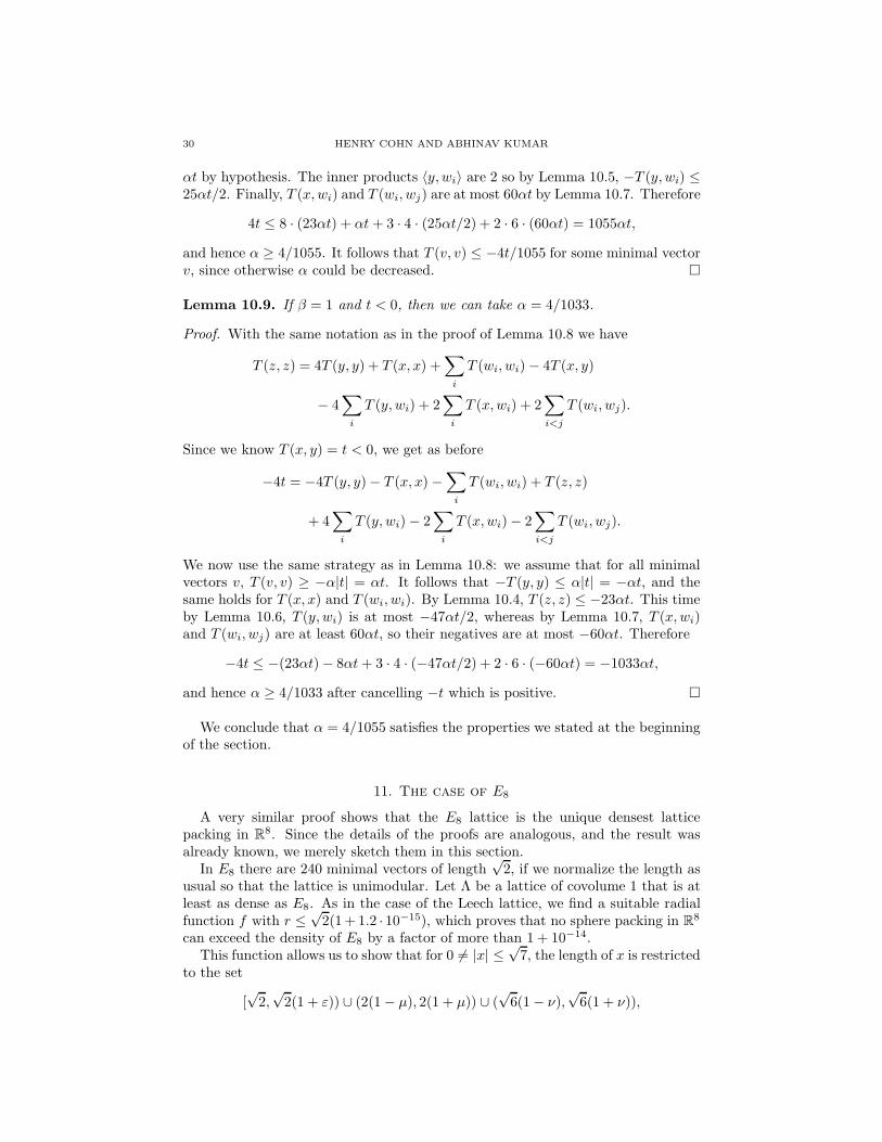
30 HENRY COHN AND ABHINAV KUMAR
αt by hypothesis. The inner products 〈y, wi〉 are 2 so by Lemma 10.5, −T (y, wi) ≤25αt/2. Finally, T (x, wi) and T (wi, wj) are at most 60αt by Lemma 10.7. Therefore
4t ≤ 8 · (23αt) + αt + 3 · 4 · (25αt/2) + 2 · 6 · (60αt) = 1055αt,
and hence α ≥ 4/1055. It follows that T (v, v) ≤ −4t/1055 for some minimal vectorv, since otherwise α could be decreased. �
Lemma 10.9. If β = 1 and t < 0, then we can take α = 4/1033.
Proof. With the same notation as in the proof of Lemma 10.8 we have
T (z, z) = 4T (y, y) + T (x, x) +∑
i
T (wi, wi) − 4T (x, y)
− 4∑
i
T (y, wi) + 2∑
i
T (x, wi) + 2∑
i<j
T (wi, wj).
Since we know T (x, y) = t < 0, we get as before
−4t = −4T (y, y) − T (x, x) −∑
i
T (wi, wi) + T (z, z)
+ 4∑
i
T (y, wi) − 2∑
i
T (x, wi) − 2∑
i<j
T (wi, wj).
We now use the same strategy as in Lemma 10.8: we assume that for all minimalvectors v, T (v, v) ≥ −α|t| = αt. It follows that −T (y, y) ≤ α|t| = −αt, and thesame holds for T (x, x) and T (wi, wi). By Lemma 10.4, T (z, z) ≤ −23αt. This timeby Lemma 10.6, T (y, wi) is at most −47αt/2, whereas by Lemma 10.7, T (x, wi)and T (wi, wj) are at least 60αt, so their negatives are at most −60αt. Therefore
−4t ≤ −(23αt) − 8αt + 3 · 4 · (−47αt/2) + 2 · 6 · (−60αt) = −1033αt,
and hence α ≥ 4/1033 after cancelling −t which is positive. �
We conclude that α = 4/1055 satisfies the properties we stated at the beginningof the section.
11. The case of E8
A very similar proof shows that the E8 lattice is the unique densest latticepacking in R
8. Since the details of the proofs are analogous, and the result wasalready known, we merely sketch them in this section.
In E8 there are 240 minimal vectors of length√
2, if we normalize the length asusual so that the lattice is unimodular. Let Λ be a lattice of covolume 1 that is atleast as dense as E8. As in the case of the Leech lattice, we find a suitable radialfunction f with r ≤
√2(1 + 1.2 · 10−15), which proves that no sphere packing in R
8
can exceed the density of E8 by a factor of more than 1 + 10−14.This function allows us to show that for 0 6= |x| ≤
√7, the length of x is restricted
to the set
[√
2,√
2(1 + ε)) ∪ (2(1 − µ), 2(1 + µ)) ∪ (√
6(1 − ν),√
6(1 + ν)),

OPTIMALITY AND UNIQUENESS OF THE LEECH LATTICE AMONG LATTICES 31
where we have
ε = 1.45 · 10−13,
µ = 1.03 · 10−6, and
ν = 4.44 · 10−6.
The details of this calculation are in the accompanying PARI file E8verifyf.txt.All the remaining calculations from this point on for the E8 case are verified in theMaple file E8rest.txt.
Define a nearly minimal vector to be a vector with length in [√
2,√
2(1 + ε)].We form a spherical code by rescaling the nearly minimal vectors to lie on the unitsphere S7.
We use the polynomial
fε(x) = (x + 1)
(x +
1
2
)2
x2
(x −
(1 − 1
2(1 + ε)2
))
to show as before that there are at most 240 nearly minimal vectors. Similarly, theanalogue of Lemma 4.4 goes through with a different function defined on R
8, andproves that there are exactly 240 nearly minimal vectors.
11.1. Spherical code. The analogue of Section 5 is that all the inner productsbetween the normalized nearly minimal vectors u/|u| must be either ±1 or at most6 · 10−5 from some element of the set {−1/2, 0, 1/2}. Then further analysis givesus the following better bounds.
For 〈u, v〉 ≈ 1 we have
2 − (1 + ε)2
2(1 + ε)2≤⟨
u
|u| ,v
|v|
⟩≤ (1 + ε)2 − 1
2,
whereas for 〈u, v〉 ≈ 0 we have
1 − (1 + µ)2
(1 + ε)2≤⟨
u
|u| ,v
|v|
⟩≤ (1 + ε)2 − (1 − µ)2.
We conclude that σ ≤ 8.89·10−6, where σ is the maximal error in the inner productsfrom the spherical code.
11.2. Intersection numbers. The analogue of Lemma 6.2 is easily shown usingthe polynomial fε.
Lemma 11.1. If g : S7 → R is a polynomial of total degree at most 6, then∣∣∣∣∣∑
z∈CΛ
g(z) − 240
vol(S7)
∫
S7
g(z) dz
∣∣∣∣∣ ≤ 3.48 · 10−4|g|2,
where |g|2 denotes the norm on L2(S7).
Now, since the kissing configuration of E8 is a 7-spherical design, we find thatthe intersection numbers of E8 can be obtained by solving the linear system ofequations
∑
α,β∈S
αiβjPγ(α, β) =240
vol(S7)
∫
S7
gi,j(z) dz.

32 HENRY COHN AND ABHINAV KUMAR
for i, j ∈ {0, 1, 2}, where S = {0,±1/2,±1} is the set of possible inner products.As before, we know the values of Pγ(±1, α) and Pγ(α,±1). When we perform thesame calculation for Λ, the value of
240
vol(S7)
∫
S7
gi,j(z) dz
differs by at most 30σ from the corresponding value for E8. If we apply Lemma 6.3and compute the error introduced into the system of equations by going from E8
to Λ, we get a bound of
(3.48 · 10−4
) π2
√3
+ 30σ + 240(1 + 2σ)σ < 4.4 · 10−3.
The ∞-norm of the inverse matrix is 100, from which it follows that the intersectionnumbers in Λ differ from those in E8 by at most 0.44. Because that number is lessthan 1, they must be the same.
11.3. Association scheme. The proof of uniqueness for the Leech lattice associ-ation scheme depended only on the eutaxy of the Leech lattice and the uniquenessof its kissing arrangement. The same hold for the E8 lattice. With N = 240 andC = 4/N = 1/60 we have the following lemma.
Lemma 11.2. For every x ∈ R8,
〈x, x〉 = C
N∑
i=1
〈x, ui〉2.
The proof of the lemma is essentially the same. We then use the lemma to provethe uniqueness of the association scheme.
Theorem 11.3. There is only one 4-class association scheme with the same size,
valencies and intersection numbers as the association scheme of minimal vectors of
the E8 lattice.
The proof of the theorem involves, as before, the operator
P = 2C
(A1 +
1
2A1/2 −
1
2A−1/2 − A−1
),
which turns out to be a projection to an 8-dimensional space. Again, the proof isessentially the same as for the Leech lattice.
11.4. Inner product bounds. The inner product bounds use only the intersectionnumbers (Lemma 7.4, for which we needed the isomorphism of association schemes,deals with a case that does not occur in E8). We get almost the same bounds as inSection 7. The proofs have to be slightly modified due to the fact that the minimalnorm of the E8 lattice is 2 instead of 4 for the Leech lattice. We get the followingresult:
Lemma 11.4. Let u, v be nearly minimal vectors.
(1) For 〈u, v〉 ≈ 2 we have 2 ≤ 〈u, v〉 ≤ 2 + (5/2)ε.(2) For 〈u, v〉 ≈ 1 we have 1 − (5/2)ε ≤ 〈u, v〉 ≤ 1 + (9/2)ε.(3) For 〈u, v〉 ≈ 0 we have −7ε ≤ 〈u, v〉 ≤ 7ε.

OPTIMALITY AND UNIQUENESS OF THE LEECH LATTICE AMONG LATTICES 33
11.5. A basis of nearly minimal vectors. The proof that there is a basis ofnearly minimal vectors is completely analogous. Consider the basis of minimalvectors
1 1 0 0 0 0 0 01 −1 0 0 0 0 0 00 1 −1 0 0 0 0 00 0 1 −1 0 0 0 00 0 0 1 −1 0 0 00 0 0 0 1 −1 0 00 0 0 0 0 1 −1 0
1/2 1/2 1/2 1/2 1/2 1/2 1/2 1/2
of E8, where the row vectors are the basis elements. Then the corresponding vectorsin Λ (via an isomorphism of association schemes) can be shown to be a basis for Λ.
11.6. Computing α. One first proves an analogue of Lemma 10.1 by consideringthe vectors wi = (0, . . . , 1, 1, . . . , 0) and vi = (0, . . . , 1,−1, . . . , 0) where the i andi + 1 coordinates are nonzero, for i ∈ {1, 3, 5, 7}.
The analogue of Lemma 10.2 is immediate:
Lemma 11.5. Let v1, . . . , v8 be orthogonal minimal vectors in the E8 lattice. If∑i,j si,jti,j = 0, then
8∑
i=1
T (vi) = 0.
We then proceed to use these lemmas as before to prove bounds on α.
Lemma 11.6. With the same notation for β and t as before, we have the following
bounds:
(1) If β = 2 and t < 0 then we can take α = 1.(2) If β = 2 and t > 0 then we can take α = 1/7.(3) If β = 1 and t < 0 then we can take α = 2/9.(4) If β = 1 and t > 0 then we can take α = 2/15.(5) If β = 0 then we can take α = 1/20.
In fact, the greatest possible value of α is 1/7, and that can be rigorously provedby computer calculations. (The linear programs are small enough that one can solvethem using exact rational arithmetic. The Maple file E8seventh.txt contains thecalculations.) However, the weaker bound of 1/20 will suffice.
11.7. Local optimality of E8. The proofs of perfection and eutaxy of E8 closelyparallel those for the Leech lattice. The Gram matrix for the basis of E8 that wechose above is small enough that we can compute all its minors quickly. We findthat for 0 < ρ < 10−3,
Dρ ≥ 1 − ρ2(7936 + 21162√
3ρ + 84256ρ2 + 47300√
5ρ3
+ 74088ρ4 + 10290√
7ρ5 + 4096ρ6)
≥ 1 − 7973ρ2.
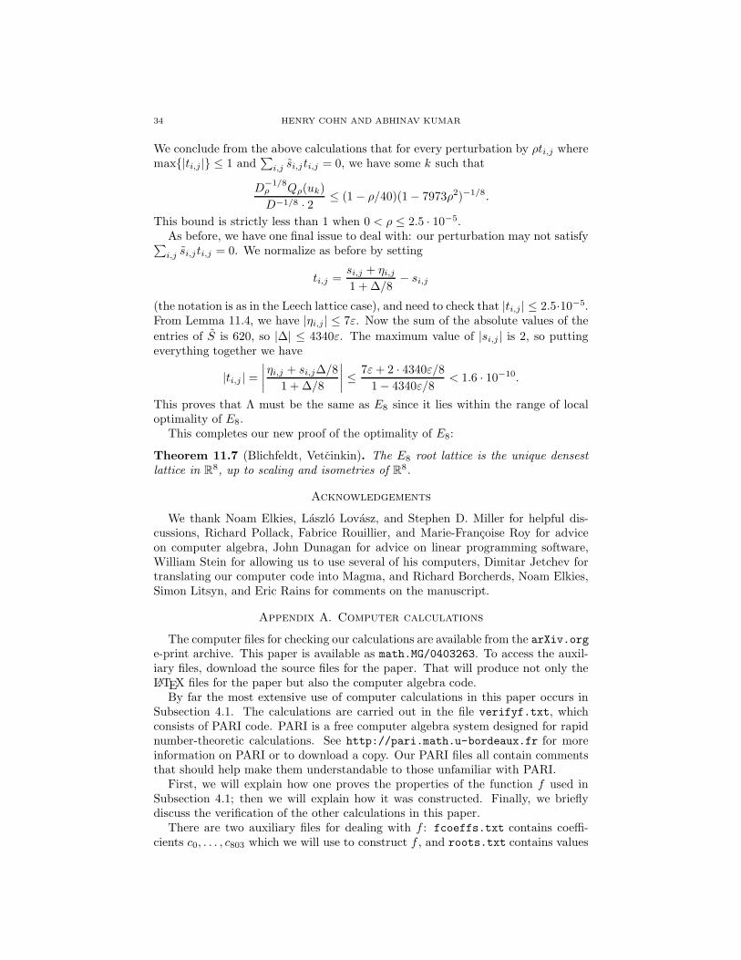
34 HENRY COHN AND ABHINAV KUMAR
We conclude from the above calculations that for every perturbation by ρti,j wheremax{|ti,j |} ≤ 1 and
∑i,j si,jti,j = 0, we have some k such that
D−1/8ρ Qρ(uk)
D−1/8 · 2 ≤ (1 − ρ/40)(1 − 7973ρ2)−1/8.
This bound is strictly less than 1 when 0 < ρ ≤ 2.5 · 10−5.As before, we have one final issue to deal with: our perturbation may not satisfy∑i,j si,jti,j = 0. We normalize as before by setting
ti,j =si,j + ηi,j
1 + ∆/8− si,j
(the notation is as in the Leech lattice case), and need to check that |ti,j | ≤ 2.5·10−5.From Lemma 11.4, we have |ηi,j | ≤ 7ε. Now the sum of the absolute values of the
entries of S is 620, so |∆| ≤ 4340ε. The maximum value of |si,j | is 2, so puttingeverything together we have
|ti,j | =
∣∣∣∣ηi,j + si,j∆/8
1 + ∆/8
∣∣∣∣ ≤7ε + 2 · 4340ε/8
1 − 4340ε/8< 1.6 · 10−10.
This proves that Λ must be the same as E8 since it lies within the range of localoptimality of E8.
This completes our new proof of the optimality of E8:
Theorem 11.7 (Blichfeldt, Vetcinkin). The E8 root lattice is the unique densest
lattice in R8, up to scaling and isometries of R
8.
Acknowledgements
We thank Noam Elkies, Laszlo Lovasz, and Stephen D. Miller for helpful dis-cussions, Richard Pollack, Fabrice Rouillier, and Marie-Francoise Roy for adviceon computer algebra, John Dunagan for advice on linear programming software,William Stein for allowing us to use several of his computers, Dimitar Jetchev fortranslating our computer code into Magma, and Richard Borcherds, Noam Elkies,Simon Litsyn, and Eric Rains for comments on the manuscript.
Appendix A. Computer calculations
The computer files for checking our calculations are available from the arXiv.orge-print archive. This paper is available as math.MG/0403263. To access the auxil-iary files, download the source files for the paper. That will produce not only theLATEX files for the paper but also the computer algebra code.
By far the most extensive use of computer calculations in this paper occurs inSubsection 4.1. The calculations are carried out in the file verifyf.txt, whichconsists of PARI code. PARI is a free computer algebra system designed for rapidnumber-theoretic calculations. See http://pari.math.u-bordeaux.fr for moreinformation on PARI or to download a copy. Our PARI files all contain commentsthat should help make them understandable to those unfamiliar with PARI.
First, we will explain how one proves the properties of the function f used inSubsection 4.1; then we will explain how it was constructed. Finally, we brieflydiscuss the verification of the other calculations in this paper.
There are two auxiliary files for dealing with f : fcoeffs.txt contains coeffi-cients c0, . . . , c803 which we will use to construct f , and roots.txt contains values

OPTIMALITY AND UNIQUENESS OF THE LEECH LATTICE AMONG LATTICES 35
r0, . . . , r200 that are nearly roots (meaning the polynomial is very near 0 at thoselocations, although in fact no real roots are nearby, except near r0).
The file verifyf.txt carries out the following verifications. Let
(A.1) f0(z) =
803∑
i=0
cii!L11i (z).
Define f : R24 → R by f(x) = f0(2π|x|2)e−π|x|2/103000. (The denominator of
103000 makes the coefficients ci integers, which is convenient.) The value of r usedin Subsection 4.1 satisfies 2πr2 = r0.
We first need to check that f(x) ≤ 0 for |x| ≥ r, which is equivalent to f0(z) ≤0 for z ≥ r0. In principle one could check this straightforwardly using Sturm’stheorem, but that takes a tremendous amount of time for such a huge polynomial.Instead, we will use Descartes’ rule of signs in a somewhat complicated way thatmay not appear a priori superior, but works overwhelmingly better in practice: thenumber of roots of a polynomial p in the interval (a, b) is at most the number ofsign changes in the coefficients of
p
(a + bz
1 + z
)(1 + z)deg(p),
and is congruent to it modulo 2. For (a,∞) one can simply use p(a + z). Thisresult is sometimes known as Jacobi’s rule of signs (see Corollary 10.1.13 in [RS,p. 320]).
We check using Jacobi’s rule of signs that f0 has no roots in (⌈r200⌉,∞) or(⌈ri⌉, ⌊ri+1⌋) for 1 ≤ i ≤ 199 (and also check that it does not vanish at the end-points), and that it has exactly one root in (0, ⌊r1⌋). Then we must check that itdoes not vanish on [⌊ri⌋, ⌈ri⌉] with 1 ≤ i ≤ 200, and that its one root is less thanr0 (for that we simply compute the sign of f0(r0)).
Dealing with the intervals [⌊ri⌋, ⌈ri⌉] is a little more difficult. We use Jacobi’srule of signs to check that f ′′
0 has no roots on these intervals, so f ′0 is monotonic
and has at most one root in each. We then check that f ′0(ri − 10−350) > 0 and
f ′0(ri+10−350) < 0, so the maximum of f0 must occur within 10−350 of ri. However,
|f ′0(ri ± 10−350)| ≤ 103285,
from which it follows (by the mean value theorem and the monotonicity of f ′0) that
∣∣∣∣f0(ri) − maxx∈[⌊ri⌋,⌈ri⌉]
f0(x)
∣∣∣∣ ≤ 10−350 · 103285 = 102935.
Because |f0(ri)| ≤ −102945, f0 has no roots in [⌊ri⌋, ⌈ri⌉].To make the proof more efficient, we arrange the calculations to ensure that only
integer arithmetic is used, so that PARI does not spend time reducing fractions tolowest terms. (That explains why the coefficients in (A.1) are multiplied by i!.)
Dealing with f is similar, but of course it uses the polynomial
h0(z) =
803∑
i=0
(−1)icii!L11i (z)
instead of f0, and in this case r0 plays the same role as r1, . . . , r200 do (rather thanbeing treated differently, as above).

36 HENRY COHN AND ABHINAV KUMAR
All that remains is to check f(0) = f(0) = 1, which is true because f0(0) =h0(0) = 103000. These calculations suffice for the proof that no sphere packing canbe more than a factor of 1 + 1.65 · 10−30 times denser than Λ24. However, Proposi-tion 4.3 requires more detailed information on the values of f . In verifyf.txt wecheck these inequalities using
351∑
i=0
(−z)i
i!≤ e−z ≤
350∑
i=0
(−z)i
i!
for 0 ≤ z ≤ 60, as well as rational upper and lower bounds for π, to avoid havingto deal with irrational numbers.
Unfortunately the file verifyf.txt cannot address where f comes from (it takesfar longer to locate f than to verify its properties). The construction is based onthe numerical technique described in Section 7 of [CE], which describes functionsvia forced double root locations that are then repeatedly perturbed until they reacha local optimum. Instead of this straightforward optimization algorithm we imple-mented a high-dimensional version of Newton’s method (which locates a root of thederivative of f(2) as an implicit function of the forced double roots—this is valuablebecause f(2) is roughly proportional to |r − 2|). We arrived at 200 forced doubleroots, whose locations are specified in roots.txt. The next step of the methodfrom [CE] also caused trouble: solving for the polynomial with those forced roots.Exact rational arithmetic was immensely time-consuming and produced huge de-nominators. Instead, we carried out high-precision floating point arithmetic androunded the result to within 10−3000. That could ruin the sign conditions on f
and f , by turning a double root into a pair of nearby single roots, so instead of
solving for actual double roots we required that f and f should stay slightly on thecorrect side of 0. That does not greatly change the resulting bounds, and leads tothe function f used in this paper.
Lemma 4.4 requires the second largest amount of computation to check, al-though far less than Subsection 4.1. The file verifyg.txt and the auxiliary filegcoeffs.txt deal with it in a fairly straightforward way.
The calculations required for (9.2) and (9.3) are dealt with in verifygram.txt.Finally, the file verifyrest.txt verifies all remaining calculations in the paper
for the Leech lattice case. Many of the calculations in this file could be checked byhand, but that would be unpleasant and error-prone. Instead of PARI code, thisfile contains Maple code. Maple is less efficient but more flexible, and it seemedeasiest to use it for these calculations.
Our computer calculations are completely rigorous, in the sense that they arecarried out using exact arithmetic and thus avoid traps such as round-off error.Nevertheless, we cannot eliminate the possibility of a hardware error or a bug insoftware beyond our control, such as the operating system or computer algebraprogram. Under these circumstances, even assuming our programs are correctlywritten they may return incorrect results. This possibility appears quite unlikely,and we do not consider it a serious worry. However, we have addressed it byasking Dimitar Jetchev to translate our programs into the Magma computer algebrasystem. His translation is contained in the file magmacode.txt. Using it, we haveindependently checked our calculations on a different type of processor, a differentcomputer algebra system, and a different operating system.

OPTIMALITY AND UNIQUENESS OF THE LEECH LATTICE AMONG LATTICES 37
We have also documented our calculations for the E8 proof. The details can befound in the files E8verifyf.txt and E8rest.txt. We include fewer comments inthese files than in the others, because their structure is parallel to the Leech latticecase. The file E8seventh.txt contains a proof that α = 1/7 works in the E8 case,although we do not require that for the proof of Theorem 11.7.
Appendix B. Background
In this appendix we collect brief definitions and descriptions of a few of theprincipal objects and techniques used in this paper.
An even unimodular lattice Λ ⊂ Rn is a lattice such that |Λ| = 1, 〈x, y〉 ∈ Z
for all x, y ∈ Λ, and 〈x, x〉 ∈ 2Z for all x ∈ Λ. Such lattices exist only when n isa multiple of 8. Up to isometries of R
n, the unique example when n = 8 is E8,and there are 24 examples in R
24, among which the Leech lattice is the unique onecontaining no vectors of length
√2. See [CS2, p. 48] for more information.
A spherical code of minimal angle ϕ in the unit sphere Sn−1 is a collectionC ⊂ Sn−1 of points such that 〈x, y〉 ≤ cosϕ for all x, y ∈ C with x 6= y. In otherwords, no two distinct points of C form an angle smaller than ϕ centered at theorigin. Spherical codes are to Sn−1 as binary error-correcting codes are to {0, 1}n,or as sphere packings are to R
n.The most important approach to bounding the size of spherical codes is linear
programming bounds (due to Delsarte [D]; see Chapter 9 of [CS2] for an exposition).These bounds rely on the following property of the ultraspherical polynomials,which follows from Lemma 6.1: if λ = n/2−1, then for each finite subset C ⊂ Sn−1,
∑
x,y∈C
Cλi (〈x, y〉) ≥ 0.
Suppose f0, . . . , fd ≥ 0, and that f(z) =∑d
i=0 fiCλi (z) satisfies f(z) ≤ 0 for z ∈
[−1, cosϕ]. Then every spherical code C in Sn−1 with minimal angle ϕ has sizebounded by |C| ≤ f(1)/f0 (assuming f0 6= 0). The proof is simple:
|C|f(1) =∑
x∈C
f(〈x, x〉)
≥∑
x,y∈C
f(〈x, y〉)
=∑
x,y∈C
f0 +
d∑
i=1
fi
∑
x,y∈C
Cλi (〈x, y〉)
≥∑
x,y∈C
f0
= |C|2f0.
The most dramatic application of the linear programming bounds for sphericalcodes is the solution of the kissing problem in R
8 and R24: how many unit balls can
be placed tangent to a central unit ball so that their interiors do not overlap? Thiscondition amounts to saying that the points of tangency form a spherical code withminimal angle π/3. In R
8 the answer is 240, and in R24 the answer is 196560. The
codes are formed from the minimal vectors in E8 and the Leech lattice, respectively

38 HENRY COHN AND ABHINAV KUMAR
(of course the radius of the sphere involved differs in the two examples). Optimalityfollows from the linear programming bounds by taking
f(z) = (z + 1)
(z +
1
2
)2
z2
(z − 1
2
)
in R8 and
f(z) = (z + 1)
(z +
1
2
)2(z +
1
4
)2
z2
(z − 1
4
)2(z − 1
2
)
in R24. This most remarkable fact was discovered independently by Levenshtein
[Lev] and by Odlyzko and Sloane [OS].A spherical t-design in Sn−1 is a non-empty finite subset D of Sn−1 such that
for every polynomial f : Rn → R of total degree at most t,
1
|D|∑
x∈D
f(x) =1
vol(Sn−1)
∫
Sn−1
f(x) dx.
In other words, the average of f over D equals its average over the entire sphere.The minimal vectors of the Leech lattice form a spherical 11-design, and those ofE8 form a spherical 7-design.
A k-class association scheme is a set A together with a partition
A2 = A0 ∪ · · · ∪ Ak
such that A0 = {(x, x) : x ∈ A}, (x, y) ∈ Ai iff (y, x) ∈ Ai, and the followingproperty holds. Fix ℓ, m, and n in Z∩ [0, k]; then for all x, y ∈ A with (x, y) ∈ Aℓ,there are the same number Pℓ(m, n) of z ∈ A such that (x, z) ∈ Am and (y, z) ∈ An.(That is, Pℓ(m, n) depends only on ℓ, m, and n, and not on x and y.) These numbersare called the intersection numbers of the association scheme. When ℓ = 0 andm = n they are also called valencies . In the body of the paper we modify thisnotation slightly for the association scheme CΛ (in a trivial way): we label theclasses with the corresponding inner products in C24, and use these labels in thenotation for the intersection numbers.
References
[AAR] G. Andrews, R. Askey, and R. Roy, Special Functions, Cambridge University Press, 1999.[BS] E. Bannai and N. J. A. Sloane, Uniqueness of certain spherical codes, Canad. J. Math. 33
(1981), 437–449.[Ba] E. S. Barnes, The complete enumeration of extreme senary forms, Phil. Transact. Royal
Soc. London A 249 (1957), 461–506.[Bl] H. F. Blichfeldt, The minimum values of positive quadratic forms in six, seven and eight
variables, Math. Z. 39 (1935), 1–15. Available from the Gottinger Digitalisierungszentrumat http://gdz.sub.uni-goettingen.de .
[BH] A. E. Brouwer and W. H. Haemers, Association schemes, in R. Graham, M. Grotschel,and L. Lovasz, eds., Handbook of Combinatorics, Volume I, Elsevier, 1995, 747–771.
[Ch] T. W. Chaundy, The arithmetic minima of positive quadratic forms, Quart. J. Math. 17
(1946), 166–192.[Co] H. Cohn, New upper bounds on sphere packings II , Geom. Topol. 6 (2002), 329–353,
arXiv:math.MG/0110010.
[CE] H. Cohn and N. Elkies, New upper bounds on sphere packings I , Annals of Mathematics157 (2003), 689–714, arXiv:math.MG/0110009.
[CS1] J. Conway and N. J. A. Sloane, Laminated lattices, Annals of Mathematics 116 (1982),593–620.

OPTIMALITY AND UNIQUENESS OF THE LEECH LATTICE AMONG LATTICES 39
[CS2] J. Conway and N. J. A. Sloane, Sphere Packings, Lattices and Groups, third edition,Springer-Verlag, 1999.
[D] P. Delsarte, Bounds for unrestricted codes, by linear programming, Philips Res. Reports27 (1972), 272–289.
[DGS] P. Delsarte, J. Goethals, and J. Seidel, Spherical codes and designs, Geometriae Dedicata6 (1977), 363–388.
[E1] N. Elkies, Mordell-Weil lattices incharacteristic 2, II. The Leech lattice as a Mordell-Weillattice, Invent. Math. 128 (1997), 1–8.
[E2] N. Elkies, Lattices, linear codes, and invariants, Notices Amer. Math. Soc. 47 (2000),1238–1245 and 1382–1391.
[G] C. F. Gauss, Untersuchungen uber die Eigenschaften der positiven ternaren quad-ratischen Formen von Ludwig August Seeber , Gottingische gelehrte Anzeigen, July9, 1831. Reprinted in Werke, Vol. 2, Konigliche Gesellschaft der Wissenschaften,Gottingen, 1863, 188–196. Available from the Gottinger Digitalisierungszentrum athttp://gdz.sub.uni-goettingen.de .
[GL] P. Gruber and C. Lekkerkerker, Geometry of Numbers, second edition, Elsevier SciencePublishers, 1987.
[H] S. Helgason, Groups and Geometric Analysis: Integral Geometry, Invariant DifferentialOperators, and Spherical Functions, Mathematical Surveys and Monographs, Volume 83,
American Mathematical Society, 2000.[HJ] R. A. Horn and C. A. Johnson, Matrix Analysis, Cambridge University Press, 1985.[K] V. P. Khavin, Methods and structure of commutative harmonic analysis, in V. P. Khavin
and N. K. Nikol’skij, eds., Commutative Harmonic Analysis I , Encyclopaedia of Mathe-matical Sciences, Volume 15, Springer-Verlag, 1991, 1–111.
[KZ1] A. Korkine and G. Zolotareff, Sur les formes quadratiques, Math. Ann. 6 (1873), 366–389.[KZ2] A. Korkine and G. Zolotareff, Sur les formes quadratiques positives, Math. Ann. 11 (1877),
242–292.[Leb] N. N. Lebedev, Special Functions and Their Applications, Dover Publications, Inc., New
York, 1972.[Lev] V. I. Levenshtein, On bounds for packings in n-dimensional Euclidean space, Soviet Math-
ematics Doklady 20 (1979), 417–421.[Ma] J. Martinet, Perfect Lattices in Euclidean Space, Springer-Verlag, 2003.[Mu] T. Muir, A Treatise on the Theory of Determinants, revised and enlarged by W. H. Metzler,
Longmans, Green and Company, 1933; reprinted by Dover Publications, 2003.[OS] A. M. Odlyzko and N. J. A. Sloane, New bounds on the number of unit spheres that
can touch a unit sphere in n dimensions, Journal of Combinatorial Theory A 26 (1979),210–214.
[RS] Q. I. Rahman and G. Schmeisser, Analytic Theory of Polynomials, Oxford UniversityPress, 2002.
[T] T. M. Thompson, From Error-Correcting Codes through Sphere Packings to SimpleGroups, Mathematical Association of America, 1983.
[Ve] N. M. Vetcinkin, Uniqueness of classes of positive quadratic forms on which values of theHermite constant are attained for 6 ≤ n ≤ 8, in Geometry of positive quadratic forms,Trudy Math. Inst. Steklov. 152 (1980), 34–86. English translation in Proc. Steklov Inst.Math. 152 (1982), 37–95.
[Vo] G. Voronoi, Proprietes des formes quadratiques positives parfaites, J. Reine Angew. Math.133 (1908), 97–178.
Microsoft Research, One Microsoft Way, Redmond, WA 98052-6399
Current address: Microsoft Research New England, One Memorial Drive, Cambridge, MA02142
E-mail address: [email protected]
Department of Mathematics, Harvard University, Cambridge, MA 02138
Current address: Department of Mathematics, Massachusetts Institute of Technology, Cam-bridge, MA 02139
E-mail address: [email protected]