
Existence and uniqueness of solutions to dynamic models ...
60
Existence and uniqueness of solutions to dynamic models with occasionally binding constraints. Tom D. Holden , School of Economics, University of Surrey 1 Abstract: We present the first necessary and sufficient conditions for there to be a unique perfect-foresight solution to an otherwise linear dynamic model with occasionally binding constraints, given a fixed terminal condition. We derive further results on the existence of a solution in the presence of such terminal conditions. These results give determinacy conditions for models with occasionally binding constraints, much as Blanchard and Kahn (1980) did for linear models. In an application, we show that widely used New Keynesian models with endogenous states possess multiple perfect foresight equilibrium paths when there is a zero lower bound on nominal interest rates, even when agents believe that the central bank will eventually attain its long-run, positive inflation target. This illustrates that a credible long-run inflation target does not render the Taylor principle sufficient for determinacy in the presence of the zero lower bound. However, we show that price level targeting does restore determinacy providing agents believe that inflation will eventually be positive. Keywords: occasionally binding constraints, zero lower bound, existence, uniqueness, price targeting, Taylor principle, linear complementarity problem JEL Classification: C62, E3, E4, E5 This version: 23 August 2017 The latest version of this paper may be downloaded from: https://github.com/tholden/dynareOBC/raw/master/TheoryPaper.pdf 1 Contact address: School of Economics, FASS, University of Surrey, Guildford, GU2 7XH, England Contact email: [email protected] Web-site: http://www.tholden.org/ The author would particularly like to thank Michael Paetz for joint work on an earlier algorithm for simulating models with occasionally binding constraints. Additionally, the author would like to thank the participants in numerous seminars at which versions of this paper were presented. Further special thanks are due to the following individuals for helpful discussions: Gary Anderson, Martin M. Andreasen, Paul Beaurdry, Saroj Bhattarai, Charles Brendon, Zsolt Csizmadia, Oliver de Groot, Michael B. Devereux, Bill Dupor, Roger Farmer, Michael Funke, William T. Gavin, Fabio Ghironi, Andy Glover, Luca Guerrieri, Pablo Guerrón-Quintana, Matteo Iacoviello, Tibor Illés, Michel Juillard, Hong Lan, Paul Levine, Jesper Lindé, Albert Marcet, Enrique Martinez-Garcia, Antonio Mele, Alexander Meyer-Gohde, Adrienn Nagy, Matthias Paustian, Jesse Perla, Frank Portier, Søren Ravn, Alexander Richter, Chris Sims, Jonathan Swarbrick, Simon Wren-Lewis and Carlos Zarazaga. Financial support provided to the author by the ESRC and the EC is also greatly appreciated. Furthermore, the author gratefully acknowledges the use of the University of Surrey FASS cluster for the numerical computations performed in this paper, and the University of Washington for providing the office space in which some of this paper was written. The research leading to these results has received funding from the European Community’s Seventh Framework Programme (FP7/2007-2013) under grant agreement “Integrated Macro-Financial Modelling for Robust Policy Design” (MACFINROBODS, grant no. 612796).
-
Upload
khangminh22 -
Category
Documents
-
view
1 -
download
0
Transcript of Existence and uniqueness of solutions to dynamic models ...

Existence and uniqueness of solutions to dynamic models with occasionally binding constraints.
Tom D. Holden, School of Economics, University of Surrey 1 Abstract: We present the first necessary and sufficient conditions for there to be a unique perfect-foresight solution to an otherwise linear dynamic model with occasionally binding constraints, given a fixed terminal condition. We derive further results on the existence of a solution in the presence of such terminal conditions. These results give determinacy conditions for models with occasionally binding constraints, much as Blanchard and Kahn (1980) did for linear models. In an application, we show that widely used New Keynesian models with endogenous states possess multiple perfect foresight equilibrium paths when there is a zero lower bound on nominal interest rates, even when agents believe that the central bank will eventually attain its long-run, positive inflation target. This illustrates that a credible long-run inflation target does not render the Taylor principle sufficient for determinacy in the presence of the zero lower bound. However, we show that price level targeting does restore determinacy providing agents believe that inflation will eventually be positive. Keywords: occasionally binding constraints, zero lower bound, existence, uniqueness, price targeting, Taylor principle, linear complementarity problem JEL Classification: C62, E3, E4, E5
This version: 23 August 2017
The latest version of this paper may be downloaded from:
https://github.com/tholden/dynareOBC/raw/master/TheoryPaper.pdf
1 Contact address: School of Economics, FASS, University of Surrey, Guildford, GU2 7XH, England Contact email: [email protected] Web-site: http://www.tholden.org/ The author would particularly like to thank Michael Paetz for joint work on an earlier algorithm for simulating models with occasionally binding constraints. Additionally, the author would like to thank the participants in numerous seminars at which versions of this paper were presented. Further special thanks are due to the following individuals for helpful discussions: Gary Anderson, Martin M. Andreasen, Paul Beaurdry, Saroj Bhattarai, Charles Brendon, Zsolt Csizmadia, Oliver de Groot, Michael B. Devereux, Bill Dupor, Roger Farmer, Michael Funke, William T. Gavin, Fabio Ghironi, Andy Glover, Luca Guerrieri, Pablo Guerrón-Quintana, Matteo Iacoviello, Tibor Illés, Michel Juillard, Hong Lan, Paul Levine, Jesper Lindé, Albert Marcet, Enrique Martinez-Garcia, Antonio Mele, Alexander Meyer-Gohde, Adrienn Nagy, Matthias Paustian, Jesse Perla, Frank Portier, Søren Ravn, Alexander Richter, Chris Sims, Jonathan Swarbrick, Simon Wren-Lewis and Carlos Zarazaga. Financial support provided to the author by the ESRC and the EC is also greatly appreciated. Furthermore, the author gratefully acknowledges the use of the University of Surrey FASS cluster for the numerical computations performed in this paper, and the University of Washington for providing the office space in which some of this paper was written. The research leading to these results has received funding from the European Community’s Seventh Framework Programme (FP7/2007-2013) under grant agreement “Integrated Macro-Financial Modelling for Robust Policy Design” (MACFINROBODS, grant no. 612796).

Page 1 of 39
1. Introduction
Models with occasionally binding constraints are ubiquitous in modern macroeconomics, yet the profession has few theoretical tools for understanding the types of multiplicity they support. This is particularly relevant for the conduct of monetary policy, as the theoretical results on determinacy that justify the Taylor principle do not apply in models with occasionally binding constraints (OBCs), such as the zero lower bound (ZLB) on nominal interest rates. Since hitting the ZLB is associated with particularly poor economic outcomes, large welfare gains are available if equilibria featuring jumps to the ZLB can be ruled out.
In this paper, we develop theoretical tools for understanding the behaviour of otherwise linear models with occasionally binding constraints. We will provide the first necessary and sufficient conditions for there always to be a unique perfect foresight solution, returning to a given steady-state, in an otherwise linear model with occasionally binding constraints. These generalise the seminal results of Blanchard & Kahn (1980) for the linear case. Moreover, we show that these conditions are not satisfied by standard New Keynesian (NK) models.
Furthermore, we will provide both necessary conditions and sufficient conditions for there to always exist a perfect foresight solution, returning to a given steady-state, to an otherwise linear model with occasionally binding constraints. We also give existence conditions that are conditional on the economy’s initial state. When no solution exists in some states, as we show to be the case in standard NK models, this implies that the model must converge to some alternative steady-state, if it has a solution at all. We note that while in the fully linear case, rational expectations and perfect-foresight solutions coincide, in the otherwise linear case considered here, this will not be the case. However, since under mild assumptions there are weakly more solutions under rational expectations than under perfect foresight,2 our results imply lower bounds on the number of solutions under rational expectations.
As was observed by Benhabib, Schmitt-Grohé & Uribe (2001a; 2001b), in the presence of OBCs, there are often multiple steady-states. For example, a model with a ZLB on nominal interest rates and Taylor rule monetary policy when away from the bound will have an additional deflationary steady-state in which nominal interest rates are zero. Such multiple steady-states can sustain multiple equilibria and sunspots if agents are switching beliefs about the point to which the economy would converge without future uncertainty.3
However, the central banks of most major economies have announced (positive) inflation targets. Thus, convergence to a deflationary steady-state would represent a spectacular failure to hit the target. As argued by Christiano and Eichenbaum (2012), a central bank may rule out the deflationary equilibria in practice by switching to a money growth rule following severe
2 This is proven in Appendix E, online. 3 The consequences of indeterminacy of this kind has been explored by Schmitt-Grohé & Uribe (2012), Mertens & Ravn (2014) and Aruoba, Cuba-Borda & Schorfheide (2014), amongst others.

Page 2 of 39
deflation, along the lines of Christiano & Rostagno (2001). Furthermore, Richter & Throckmorton (2015) and Gavin et al. (2015) present evidence that the deflationary equilibrium is unstable4 under rational expectations if shocks are large enough, making it much harder for agents to coordinate upon it. This suggests agents should believe that inflation will eventually return to the vicinity of its target, and they ought to place zero probability on paths converging to deflation. Such beliefs appear to be in line with the empirical evidence of Gürkaynak, Levin & Swanson (2010). If agents’ beliefs satisfy these restrictions, then the kind of multiplicity discussed in the previous paragraph is ruled out. It is an important question, then, whether there are still multiple equilibria even when all agents believe that in the long-run, the economy will return to a particular steady-state. It is on such equilibria that we focus in this paper.
To understand why multiplicity is still possible even with the terminal condition fixed, suppose that somehow the model’s agents knew that from next period onwards, the economy would be away from the bound. Then, in an otherwise linear model, expectations of next period’s outcomes would be linear in today’s variables. However, substituting out these expectations does not leave a linear system in today’s variables, due to the occasionally binding constraint. For some models, this non-linear system will have two solutions, with one featuring a slack constraint, and the other having a binding constraint. Thus, even though the rule for forming expectations is pinned down, there may still be multiple possible outcomes today. Without the assumption that next period the economy is away from the bound, the scope for multiplicity is even richer, and there may be infinitely many solutions.
In an application, we show that multiplicity of perfect-foresight paths is the rule in otherwise linear New Keynesian models with endogenous state variables (e.g. price dispersion) and a ZLB. This means that even when agents’ long-run expectations are pinned down, there is still multiplicity of equilibria, implying the Taylor principle is not sufficient for determinacy in the presence of occasionally binding constrains. Indeed, in these models, there are conditions under which the economy has one return path that never hits the ZLB, and another that does, so there may be multiplicity even when away from the bound. However, we show that under a price-targeting regime, there is a unique equilibrium path even when we impose the ZLB. Thus, if the standard arguments for the Taylor principle convince policy makers, then, given they face the ZLB, they ought to consider adopting a price level target.
We also show that for standard NK models with endogenous state variables, there is a positive probability of ending up in a state of the world (i.e. with certain state variables and shock realisations) in which there is no perfect foresight path returning to the “good” steady-state. Hence, if we suppose that in the stochastic model, agents deal with uncertainty by integrating over the space of possible future shock sequences, as in the original stochastic
4 They show that policy function iteration is not stable near the deflationary equilibria.

Page 3 of 39
extended path algorithm of Adjemian & Juillard (2013),5 then such agents would always put positive probability on tending to the “bad” steady-state. Since the second steady-state is indeterminate in NK models, this implies global indeterminacy by a backwards induction argument. Once again though, price level targeting would be sufficient to restore determinacy.
The most relevant prior work for ours is that of Brendon, Paustian & Yates (2013; 2016), henceforth abbreviated to BPY. Like us, these authors examined perfect foresight equilibria of NK models with terminal conditions. In BPY (2013), the authors show analytically that in a very simple NK model, featuring a response to the growth rate in the Taylor rule, there are multiple perfect-foresight equilibria when all agents believe that with probability one, in one period’s time, they will escape the bound and return to the neighbourhood of the “good” steady-state. Furthermore, in BPY (2013; 2016), the authors show numerically that in some select other models, there are multiple perfect-foresight equilibria when the economy begins at the steady-state, and all agents believe that the economy will jump to the bound, remain there for some number of periods, before leaving it endogenously, after which they believe they will never hit the bound again.
Relative to these authors, we will provide far more general theoretical results, and these will permit numerical analysis that is both more robust and less restrictive. This robustness and generality will prove crucial in showing multiplicity even in simple NK models, with entirely standard Taylor rules. For example, whereas BPY (2016) write that price-dispersion “does not have a strong enough impact on equilibrium allocations for the sort of propagation that we need”, we show that the presence of price dispersion is sufficient for multiplicity. Likewise, whereas BPY (2013; 2016) find a much weaker role for multiplicity when the monetary rule does not include a response to the growth rate of output, our findings of multiplicity will not be at all dependent on such a response, implying very different policy prescriptions.
Further relevant papers are discussed in Section 6, in the course of examining our results. The rest of our paper is structured as follows. In the following section, Section 2, we present the key representation result which enables us to examine existence and uniqueness in models with OBCs and terminal conditions via examining the properties of linear complementarity problems. Section 3 introduces a simple example New Keynesian model with multiplicity, and provides further intuition. Next, Section 4 presents our main results on existence and uniqueness. We then apply these results to further NK models in Section 5. Section 7 concludes. All files needed for the replication of this paper’s numerical results are included in the author’s DynareOBC toolkit, which implements an algorithm for simulating models with occasionally binding constraints that we discuss in a companion paper (Holden 2016), as well as checking the existence and uniqueness conditions that we will discuss here. 5 Strictly, this is not fully rational, as it is equivalent to assuming that agents act as if the uncertainty in all future periods would be resolved next period. However, in practice this appears to be a close approximation to full rationality, as demonstrated by Holden (2016). The authors of the original stochastic path method now have a more complicated version that is fully consistent with rationality (Adjemian & Juillard 2016).

Page 4 of 39
2. Representation result
In this section, we present the representation result that establishes an equivalence between solutions of a DSGE model with occasionally binding constraints, and solutions of a linear complementarity problem. The key idea behind the result’s proof is that an OBC provides a source of endogenous news about the future. If a shock hits, driving the economy to the bound in some future periods, then, in those future periods, the (lower) bounded variable will be higher that it would be otherwise.6 Hence, any shock that causes the ZLB to be hit may be thought of as providing a source of endogenous news about future innovations to the monetary rule, of just the right magnitude needed to impose the ZLB. For example, if the size of a productivity shock is such that in the absence of the ZLB, nominal interest rates would be negative a year after the original shock, then, in the presence of the ZLB, the shock is providing endogenous news that nominal interest rates will be higher than otherwise in a year’s time.
2.1. Problem set-ups We start by defining the problem to be solved, and examining its relationship both to the
problem without OBCs, and to a related problem with news shocks to the bounded variable. In the absence of occasionally binding constraints, calculating an impulse response or
performing a perfect foresight simulation exercise in a linear DSGE model is equivalent to solving the following problem:7
Problem 1 (Linear) Suppose that 𝑥𝑥0 ∈ ℝ𝑛𝑛 is given. Find 𝑥𝑥𝑡𝑡 ∈ ℝ𝑛𝑛 for 𝑡𝑡 ∈ ℕ+ such that 𝑥𝑥𝑡𝑡 → 𝜇𝜇 as 𝑡𝑡 → ∞, and such that for all 𝑡𝑡 ∈ ℕ+:
(𝐴𝐴 + 𝐵𝐵 + 𝐶𝐶)𝜇𝜇 = 𝐴𝐴𝑥𝑥𝑡𝑡−1 + 𝐵𝐵𝑥𝑥𝑡𝑡 + 𝐶𝐶𝑥𝑥𝑡𝑡+1, (1)
Throughout this paper, we will refer to equilibrium conditions such as equation (1) as “the model”, conflating them with the optimisation problem(s) which gave rise to them. We make the following assumption in all the following:
Assumption 1 For any given 𝑥𝑥0 ∈ ℝ𝑛𝑛 , Problem 1 (Linear) has a unique solution, which (without loss of generality) takes the form 𝑥𝑥𝑡𝑡 = (𝐼𝐼 − 𝐹𝐹)𝜇𝜇 + 𝐹𝐹𝑥𝑥𝑡𝑡−1, for 𝑡𝑡 ∈ ℕ+, where 0 = 𝐴𝐴 +𝐵𝐵𝐹𝐹 + 𝐶𝐶𝐹𝐹𝐹𝐹, and where the eigenvalues of 𝐹𝐹 are strictly inside the unit circle.
6 The idea of imposing an OBC by adding news shocks is also present in Holden (2010), Hebden et al. (2011), Holden & Paetz (2012) and Bodenstein et al. (2013). Laséen & Svensson (2011) use a similar technique to impose a path of nominal interest rates, in a non-ZLB context. None of these papers formally establish our representation result. News shocks were introduced by Beaudry & Portier (2006). 7 The absence of shocks and expectations here is without loss of generality. For suppose �𝐴𝐴̂ + �̂�𝐵 + 𝐶𝐶�̂𝜇𝜇̂ = 𝐴𝐴�̂�𝑥�̂�𝑡−1 +�̂�𝐵𝑥𝑥�̂�𝑡 + 𝐶𝐶�̂�𝔼𝑡𝑡𝑥𝑥�̂�𝑡+1 + 𝐷𝐷� 𝜀𝜀𝑡𝑡, with 𝑥𝑥�̂�𝑡 → 𝜇𝜇̂ as 𝑡𝑡 → ∞, and that 𝜀𝜀𝑡𝑡 = 0 for 𝑡𝑡 > 1, as in an impulse response or perfect foresight
simulation exercise. Then, if we define 𝑥𝑥𝑡𝑡 ≔ � 𝑥𝑥�̂�𝑡𝜀𝜀𝑡𝑡+1
�, 𝜇𝜇 ≔ �𝜇𝜇̂0
�, 𝐴𝐴 ≔ �𝐴𝐴̂ 𝐷𝐷�0 0
�, 𝐵𝐵 ≔ ��̂�𝐵 00 𝐼𝐼
�, 𝐶𝐶 ≔ �𝐶𝐶̂ 00 0
�, then we are
left with a problem in the form of Problem 1 (Linear), with the extended initial condition 𝑥𝑥0 = �𝑥𝑥0̂𝜀𝜀1
� , and the
extended terminal condition 𝑥𝑥𝑡𝑡 → 𝜇𝜇 as 𝑡𝑡 → ∞. Expectations disappear as there is no uncertainty after period 0.

Page 5 of 39
Conditions (A’) and (B) from Sims’s (2002) generalisation of the standard Blanchard-Kahn (1980) conditions are necessary and sufficient for Assumption 1 to hold. Further, to avoid dealing specially with the knife-edge case of exact unit eigenvalues in the part of the model that is solved forward, here we rule it out with the subsequent assumption, which is, in any case, a necessary condition for perturbation to produce a consistent approximation to a non-linear model, and which is also necessary for the linear model to have a unique steady-state:
Assumption 2 det(𝐴𝐴 + 𝐵𝐵 + 𝐶𝐶) ≠ 0.
We are interested in models featuring occasionally binding constraints. We will concentrate on models featuring a single ZLB type constraint in their first equation, which does not bind in steady-state, and which we treat as defining the first element of 𝑥𝑥𝑡𝑡. Generalising from this special case to models with one or more fully general bounds is straightforward, and is discussed in Appendix A. First, let us write 𝑥𝑥1,𝑡𝑡, 𝐼𝐼1,⋅, 𝐴𝐴1,⋅, 𝐵𝐵1,⋅, 𝐶𝐶1,⋅ for the first row of 𝑥𝑥𝑡𝑡, 𝐼𝐼, 𝐴𝐴, 𝐵𝐵, 𝐶𝐶 (respectively) and 𝑥𝑥−1,𝑡𝑡, 𝐼𝐼−1,⋅, 𝐴𝐴−1,⋅, 𝐵𝐵−1,⋅, 𝐶𝐶−1,⋅ for the remainders. Likewise, we write 𝐼𝐼⋅,1 for the first column of 𝐼𝐼, and so on. Then, we are interested in:
Problem 2 (OBC) Suppose that 𝑥𝑥0 ∈ ℝ𝑛𝑛 is given. Find 𝑇𝑇 ∈ ℕ and 𝑥𝑥𝑡𝑡 ∈ ℝ𝑛𝑛 for 𝑡𝑡 ∈ ℕ+ such that 𝑥𝑥𝑡𝑡 → 𝜇𝜇 as 𝑡𝑡 → ∞, such that for all 𝑡𝑡 ∈ ℕ+:
𝑥𝑥1,𝑡𝑡 = max�0, 𝐼𝐼1,⋅𝜇𝜇 + 𝐴𝐴1,⋅�𝑥𝑥𝑡𝑡−1 − 𝜇𝜇� + �𝐵𝐵1,⋅ + 𝐼𝐼1,⋅��𝑥𝑥𝑡𝑡 − 𝜇𝜇� + 𝐶𝐶1,⋅�𝑥𝑥𝑡𝑡+1 − 𝜇𝜇��, �𝐴𝐴−1,⋅ + 𝐵𝐵−1,⋅ + 𝐶𝐶−1,⋅�𝜇𝜇 = 𝐴𝐴−1,⋅𝑥𝑥𝑡𝑡−1 + 𝐵𝐵−1,⋅𝑥𝑥𝑡𝑡 + 𝐶𝐶−1,⋅𝑥𝑥𝑡𝑡+1,
and such that 𝑥𝑥1,𝑡𝑡 > 0 for 𝑡𝑡 > 𝑇𝑇.
given:
Assumption 3 𝜇𝜇1 > 0.
Were it not for the max, this problem would be identical to Problem 1 (Linear), providing that Assumption 3 holds, as the existence of a 𝑇𝑇 ∈ ℕ such that 𝑥𝑥1,𝑡𝑡 > 0 for 𝑡𝑡 > 𝑇𝑇 is guaranteed by the fact that 𝑥𝑥1,𝑡𝑡 → 𝜇𝜇1 as 𝑡𝑡 → ∞. In this problem, we are implicitly ruling out any solutions which get permanently stuck at an alternative steady-state, by assuming that the terminal condition remains as before. In the monetary policy context, this amounts to assuming that the central banks’ long-run inflation target is credible. As we are assuming there is no uncertainty, the path of the endogenous variables will not necessarily match up with the path of their expectation in a richer model in which there was uncertainty, due to the non-linearity.
In many models, the occasionally binding constraint comes from the KKT conditions of an optimisation problem, which take the form 𝑧𝑧𝑡𝑡 ≥ 0 , 𝜆𝜆𝑡𝑡 ≥ 0 and 𝑧𝑧𝑡𝑡𝜆𝜆𝑡𝑡 = 0 . These may be converted into the max/min form since they are equivalent to the single equation 0 =min{𝑧𝑧𝑡𝑡, 𝜆𝜆𝑡𝑡}, which holds if and only if 𝑧𝑧𝑡𝑡 = max{0, 𝑧𝑧𝑡𝑡 − 𝜆𝜆𝑡𝑡}, an equation in the form of Problem 2 (OBC). Additionally, in Appendix D, we give an alternative procedure for converting KKT conditions into the form of Problem 2 (OBC), based on finding a “shadow” value of the constrained variable.

Page 6 of 39
We will analyse Problem 2 (OBC) with the help of solutions to the auxiliary problem:
Problem 3 (News) Suppose that 𝑇𝑇 ∈ ℕ, 𝑥𝑥0 ∈ ℝ𝑛𝑛 and 𝑦𝑦0 ∈ ℝ𝑇𝑇 is given. Find 𝑥𝑥𝑡𝑡 ∈ ℝ𝑛𝑛, 𝑦𝑦𝑡𝑡 ∈ ℝ𝑇𝑇 for 𝑡𝑡 ∈ ℕ+ such that 𝑥𝑥𝑡𝑡 → 𝜇𝜇, 𝑦𝑦𝑡𝑡 → 0, as 𝑡𝑡 → ∞, and such that for all 𝑡𝑡 ∈ ℕ+:
(𝐴𝐴 + 𝐵𝐵 + 𝐶𝐶)𝜇𝜇 = 𝐴𝐴𝑥𝑥𝑡𝑡−1 + 𝐵𝐵𝑥𝑥𝑡𝑡 + 𝐶𝐶𝑥𝑥𝑡𝑡+1 + 𝐼𝐼⋅,1𝑦𝑦1,𝑡𝑡−1, 𝑦𝑦𝑇𝑇,𝑡𝑡 = 0, ∀𝑖𝑖 ∈ {1, … , 𝑇𝑇 − 1}, 𝑦𝑦𝑖𝑖,𝑡𝑡 = 𝑦𝑦𝑖𝑖+1,𝑡𝑡−1.
This may be thought of as a version of Problem 1 (Linear) with news shocks up to horizon 𝑇𝑇 added to the first equation. By construction, the value of 𝑦𝑦𝑖𝑖,𝑡𝑡 gives the shock that in period 𝑡𝑡 is expected to arrive in 𝑖𝑖 periods. Hence, as all information is known in period 0, 𝑦𝑦𝑡𝑡,0 gives the shock that will hit in period 𝑡𝑡, i.e. 𝑦𝑦1,𝑡𝑡−1 = 𝑦𝑦𝑡𝑡,0 for 𝑡𝑡 ≤ 𝑇𝑇, and 𝑦𝑦1,𝑡𝑡−1 = 0 for 𝑡𝑡 > 𝑇𝑇.
2.2. Relationships between the problems A straightforward backwards induction argument (given in Appendix H.1, online) gives the
following helpful result:
Lemma 1 There is a unique solution to Problem 3 (News) that is linear in 𝑥𝑥0 and 𝑦𝑦0.
For future reference, let 𝑥𝑥𝑡𝑡(3,𝑘𝑘) be the solution to Problem 3 (News) when 𝑥𝑥0 = 𝜇𝜇, 𝑦𝑦0 = 𝐼𝐼⋅,𝑘𝑘 (i.e. a
vector which is all zeros apart from a 1 in position 𝑘𝑘). Then, by linearity, for arbitrary 𝑦𝑦0 the solution to Problem 3 (News) when 𝑥𝑥0 = 𝜇𝜇 is given by:
𝑥𝑥𝑡𝑡 − 𝜇𝜇 = � 𝑦𝑦𝑘𝑘,0�𝑥𝑥𝑡𝑡(3,𝑘𝑘) − 𝜇𝜇�
𝑇𝑇
𝑘𝑘=1.
Now, let 𝑀𝑀 ∈ ℝ𝑇𝑇×𝑇𝑇 satisfy: 𝑀𝑀𝑡𝑡,𝑘𝑘 = 𝑥𝑥1,𝑡𝑡
(3,𝑘𝑘) − 𝜇𝜇1, ∀𝑡𝑡, 𝑘𝑘 ∈ {1, . . , 𝑇𝑇}, (2)
i.e. 𝑀𝑀 horizontally stacks the (column-vector) relative impulse responses of the first variable to the news shocks, with the first column giving the response to a contemporaneous shock, the second column giving the response to a shock anticipated by one period, and so on. Then, this result implies that for arbitrary 𝑥𝑥0 and 𝑦𝑦0, the path of the first variable in the solution to Problem 3 (News) is given by:
�𝑥𝑥1,1:𝑇𝑇�′ = 𝑞𝑞 + 𝑀𝑀𝑦𝑦0, (3) where 𝑞𝑞 ≔ �𝑥𝑥1,1:𝑇𝑇
(1) �′ and where 𝑥𝑥𝑡𝑡
(1) is the unique solution to Problem 1 (Linear), for the given
𝑥𝑥0, i.e. 𝑞𝑞 is the path of the first variable in the absence of news shocks or bounds. 8 Since 𝑀𝑀 is not a function of either 𝑥𝑥0 or 𝑦𝑦0, equation (3) gives a highly convenient representation of the solution to Problem 3 (News).
Now let 𝑥𝑥𝑡𝑡(2) be a solution to Problem 2 (OBC) given some 𝑥𝑥0. Since 𝑥𝑥𝑡𝑡
(2) → 𝜇𝜇 as 𝑡𝑡 → ∞, there exists 𝑇𝑇′ ∈ ℕ such that for all 𝑡𝑡 > 𝑇𝑇′, 𝑥𝑥1,𝑡𝑡
(2) > 0. We assume without loss of generality that 𝑇𝑇′ ≤
𝑇𝑇. We seek to relate the solution to Problem 2 (OBC) with the one to Problem 3 (News) for an appropriate choice of 𝑦𝑦0. First, for all 𝑡𝑡 ∈ ℕ+, let:
𝑒𝑒�̂�𝑡 ≔ −�𝐼𝐼1,⋅𝜇𝜇 + 𝐴𝐴1,⋅�𝑥𝑥𝑡𝑡−1(2) − 𝜇𝜇� + �𝐵𝐵1,⋅ + 𝐼𝐼1,⋅��𝑥𝑥𝑡𝑡
(2) − 𝜇𝜇� + 𝐶𝐶1,⋅�𝑥𝑥𝑡𝑡+1(2) − 𝜇𝜇��,
8 This representation was also exploited by Holden (2010) and Holden and Paetz (2012).

Page 7 of 39
𝑒𝑒𝑡𝑡 ≔⎩�⎨�⎧𝑒𝑒�̂�𝑡 if 𝑥𝑥1,𝑡𝑡
(2) = 0
0 if 𝑥𝑥1,𝑡𝑡(2) > 0
, (4)
i.e. 𝑒𝑒𝑡𝑡 is the shock that would need to hit the first equation for the positivity constraint on 𝑥𝑥1,𝑡𝑡(2)
to be enforced. Note that by the definition of Problem 2 (OBC), 𝑒𝑒𝑡𝑡 ≥ 0 and 𝑥𝑥1,𝑡𝑡(2)𝑒𝑒𝑡𝑡 = 0, for all 𝑡𝑡 ∈
ℕ+. Then, again from a backwards induction argument, (in Appendix H.2, online) we have:
Lemma 2 For any solution, �𝑇𝑇, 𝑥𝑥𝑡𝑡(2)� to Problem 2 (OBC):
1) With 𝑒𝑒1:𝑇𝑇 as defined in equation (4) , 𝑒𝑒1:𝑇𝑇 ≥ 0 , 𝑥𝑥1,1:𝑇𝑇(2) ≥ 0 and 𝑥𝑥1,1:𝑇𝑇
(2) ∘ 𝑒𝑒1:𝑇𝑇 = 0 , where ∘
denotes the Hadamard (entry-wise) product. 2) 𝑥𝑥𝑡𝑡
(2) is also the unique solution to Problem 3 (News) with 𝑥𝑥0 = 𝑥𝑥0(2) and 𝑦𝑦0 = 𝑒𝑒1:𝑇𝑇
′ . 3) If 𝑥𝑥𝑡𝑡
(2) solves Problem 3 (News) with 𝑥𝑥0 = 𝑥𝑥0(2) and with some 𝑦𝑦0, then 𝑦𝑦0 = 𝑒𝑒1:𝑇𝑇
′ .
To use the easy solution to Problem 3 (News) to assist us in solving Problem 2 (OBC) just requires one more result. In particular, we show in Appendix H.3, online, that if 𝑦𝑦0 ∈ ℝ𝑇𝑇 is such that 𝑦𝑦0 ≥ 0, 𝑥𝑥1,1:𝑇𝑇
(3) ∘ 𝑦𝑦0′ = 0 and 𝑥𝑥1,𝑡𝑡
(3) ≥ 0 for all 𝑡𝑡 ∈ ℕ, where 𝑥𝑥𝑡𝑡(3) is the unique solution to
Problem 3 (News) when started at 𝑥𝑥0, 𝑦𝑦0, then 𝑥𝑥𝑡𝑡(3) must also be a solution to Problem 2 (OBC).
Together with Lemma 1, Lemma 2, and our representation of the solution of Problem 3 (News) from equation (3), this completes the proof of the following key theorem:
Theorem 1 The following hold: 1) Let 𝑥𝑥𝑡𝑡
(3) be the unique solution to Problem 3 (News) given 𝑇𝑇 ∈ ℕ+, 𝑥𝑥0 ∈ ℝ𝑛𝑛 and 𝑦𝑦0 ∈ ℝ𝑇𝑇. Then �𝑇𝑇, 𝑥𝑥𝑡𝑡
(3)� is a solution to Problem 2 (OBC) given 𝑥𝑥0 if and only if 𝑦𝑦0 ≥ 0 , 𝑦𝑦0 ∘�𝑞𝑞 + 𝑀𝑀𝑦𝑦0� = 0, 𝑞𝑞 + 𝑀𝑀𝑦𝑦0 ≥ 0 and 𝑥𝑥1,𝑡𝑡
(3) ≥ 0 for all 𝑡𝑡 > 𝑇𝑇.
2) Let �𝑇𝑇, 𝑥𝑥𝑡𝑡(2)� be any solution to Problem 2 (OBC) given 𝑥𝑥0. Then there exists a unique 𝑦𝑦0 ∈
ℝ𝑇𝑇 such that 𝑦𝑦0 ≥ 0 , 𝑦𝑦0 ∘ �𝑞𝑞 + 𝑀𝑀𝑦𝑦0� = 0 , 𝑞𝑞 + 𝑀𝑀𝑦𝑦0 ≥ 0 , and such that 𝑥𝑥𝑡𝑡(2) is the unique
solution to Problem 3 (News) given 𝑇𝑇, 𝑥𝑥0 and 𝑦𝑦0.
2.3. The linear complementarity representation Theorem 1 establishes that we may solve Problem 2 (OBC) by conjecturing a (sufficiently
high) value for 𝑇𝑇 and then solving the following problem:
Problem 4 (LCP) Suppose 𝑇𝑇 ∈ ℕ+, 𝑞𝑞 ∈ ℝ𝑇𝑇 and 𝑀𝑀 ∈ ℝ𝑇𝑇×𝑇𝑇 are given. Find 𝑦𝑦 ∈ ℝ𝑇𝑇 such that 𝑦𝑦 ≥ 0 , 𝑦𝑦 ∘ �𝑞𝑞 + 𝑀𝑀𝑦𝑦� = 0 and 𝑞𝑞 + 𝑀𝑀𝑦𝑦 ≥ 0 . We call this the linear complementarity problem (LCP) �𝑞𝑞, 𝑀𝑀�. (Cottle 2009)
These problems have been extensively studied, and so we can import results on the properties of LCPs to derive results on the properties of models with OBCs.
All the results in the literature on LCPs rest on properties of the matrix 𝑀𝑀, thus we would like to establish if the structure of our particular 𝑀𝑀 implies it has any special properties. Unfortunately, we prove the following result in Appendix H.4, online, which means that 𝑀𝑀’s origin implies no particular properties:

Page 8 of 39
Proposition 1 For any 𝑇𝑇 ∈ ℕ+ and ℳ ∈ ℝ𝑇𝑇×𝑇𝑇, there exists a model in the form of Problem 2 (OBC) with a number of state variables given by a quadratic in 𝑇𝑇, such that 𝑀𝑀 = ℳ for that model, where 𝑀𝑀 is defined as in equation (2), and such that for all 𝓆𝓆 ∈ ℝ𝑇𝑇 , there exists an initial state for which 𝑞𝑞 = 𝓆𝓆 , where 𝑞𝑞 is the path of the bounded variable when constraints are
ignored. (Holden 2016)
3. Intuition building results and examples
3.1. LCPs of size 1 When 𝑇𝑇 = 1, it is particularly easy to characterise the properties of LCPs. This amounts to
considering the behaviour of an economy in which everyone believes there will be at most one period at the bound. In this case, 𝑦𝑦 gives the “shock” to the bounded equation necessary to impose the bound, and 𝑀𝑀 gives the contemporaneous response of the bounded variable to an unanticipated shock: i.e. in a ZLB context, 𝑀𝑀 gives the initial jump in nominal interest rates following a standard monetary policy shock.
First, suppose that 𝑀𝑀 (a scalar as 𝑇𝑇 = 1 for now) is positive. Then, if 𝑞𝑞 > 0, for any 𝑦𝑦 ≥ 0, 𝑞𝑞 +𝑀𝑀𝑦𝑦 > 0, so by the complementary slackness condition, in fact 𝑦𝑦 = 0. Conversely, if 𝑞𝑞 ≤ 0, then there is a unique 𝑦𝑦 satisfying the complementary slackness condition given by 𝑦𝑦 = − 𝑞𝑞
𝑀𝑀 ≥ 0.
Thus, with 𝑀𝑀 > 0, there is always a unique solution to the 𝑇𝑇 = 1 LCP. With 𝑀𝑀 = 0, 𝑞𝑞 + 𝑀𝑀𝑦𝑦 =𝑞𝑞, so a solution to the LCP exists if and only if 𝑞𝑞 ≥ 0. It will be unique providing 𝑞𝑞 > 0 (by the complementary slackness condition), but when 𝑞𝑞 = 0 , any 𝑦𝑦 ≥ 0 gives a solution. Finally, suppose that 𝑀𝑀 < 0. Then, if 𝑞𝑞 > 0, there are precisely two solutions. The “standard” solution has 𝑦𝑦 = 0 , but there is an additional solution featuring a jump to the bound in which 𝑦𝑦 =− 𝑞𝑞
𝑀𝑀 > 0 . If 𝑞𝑞 = 0 , then there is a unique solution (𝑦𝑦 = 0 ) and if 𝑞𝑞 < 0 , then with 𝑦𝑦 ≥ 0 , 𝑞𝑞 +
𝑀𝑀𝑦𝑦 < 0, so there is no solution at all. Hence, the 𝑇𝑇 = 1 LCP already provides examples of cases of uniqueness, non-existence and multiplicity.
3.2. The simple Brendon, Paustian & Yates (BPY) (2013) model Brendon, Paustian & Yates (2013), henceforth BPY, provide a simple New Keynesian model
that we can use to illustrate and better understand these cases. Its equations follow: 𝑥𝑥𝑖𝑖,𝑡𝑡 = max�0,1 − 𝛽𝛽 + 𝛼𝛼∆𝑦𝑦�𝑥𝑥𝑦𝑦,𝑡𝑡 − 𝑥𝑥𝑦𝑦,𝑡𝑡−1� + 𝛼𝛼𝜋𝜋𝑥𝑥𝜋𝜋,𝑡𝑡�,
𝑥𝑥𝑦𝑦,𝑡𝑡 = 𝔼𝔼𝑡𝑡𝑥𝑥𝑦𝑦,𝑡𝑡+1 −1𝜎𝜎 �𝑥𝑥𝑖𝑖,𝑡𝑡 + 𝛽𝛽 − 1 − 𝔼𝔼𝑡𝑡𝑥𝑥𝜋𝜋,𝑡𝑡+1�,
𝑥𝑥𝜋𝜋,𝑡𝑡 = 𝛽𝛽𝔼𝔼𝑡𝑡𝑥𝑥𝜋𝜋,𝑡𝑡+1 + 𝛾𝛾𝑥𝑥𝑦𝑦,𝑡𝑡, where 𝑥𝑥𝑖𝑖,𝑡𝑡 is the nominal interest rate, 𝑥𝑥𝑦𝑦,𝑡𝑡 is the deviation of output from steady-state, 𝑥𝑥𝜋𝜋,𝑡𝑡 is the deviation of inflation from steady-state, and 𝛽𝛽 ∈ (0,1), 𝛾𝛾, 𝜎𝜎, 𝛼𝛼∆𝑦𝑦 ∈ (0, ∞), 𝛼𝛼𝜋𝜋 ∈ (1, ∞) are
parameters. The model’s only departure from the textbook three equation NK model is the presence of an output growth rate term in the Taylor rule. This introduces an endogenous state variable in a tractable manner. In Appendix H.5, online, we prove the following:
Page 9 of 39
Proposition 2 The BPY model is in the form of Problem 2 (OBC), and satisfies Assumptions 1, 2 and 3. With 𝑇𝑇 = 1, 𝑀𝑀 < 0 (𝑀𝑀 = 0) if and only if 𝛼𝛼∆𝑦𝑦 > 𝜎𝜎𝛼𝛼𝜋𝜋 (𝛼𝛼∆𝑦𝑦 = 𝜎𝜎𝛼𝛼𝜋𝜋).
Hence, by Theorem 1, when all agents believe the bound will be escaped after at most one period, if 𝛼𝛼∆𝑦𝑦 < 𝜎𝜎𝛼𝛼𝜋𝜋 , the model has a unique solution for all 𝑞𝑞, i.e. no matter what the nominal interest rate would be that period were no ZLB. If 𝛼𝛼∆𝑦𝑦 = 𝜎𝜎𝛼𝛼𝜋𝜋, then the model has a unique
solution whenever 𝑞𝑞 > 0, infinitely many solutions when 𝑞𝑞 = 0, and no solutions leaving the ZLB after one period when 𝑞𝑞 < 0. Finally, if 𝛼𝛼∆𝑦𝑦 > 𝜎𝜎𝛼𝛼𝜋𝜋 then the model has two solutions when
𝑞𝑞 > 0, one solution when 𝑞𝑞 = 0 and no solution escaping the ZLB next period when 𝑞𝑞 < 0. The mechanism here is as follows. The stronger the response to the growth rate, the more
persistent is output, as the monetary rule implies additional stimulus if output was high last period. Suppose then that there was an unexpected positive shock to nominal interest rates. Then, due to the persistence, this would lower not just output and inflation today, but also output and inflation next period. With low expected inflation, real interest rates are high, giving consumers an additional reason to save, and thus further lowering output and inflation this period and next. With sufficiently high 𝛼𝛼∆𝑦𝑦, this additional amplification is so strong that
nominal interest rates fall this period, despite the positive shock, explaining why 𝑀𝑀 may be negative.9 Now, consider varying the magnitude of the original shock. For a sufficiently large shock, interest rates would hit zero. At this point, there is no observable evidence that a shock has arrived at all, since the ZLB implies that given the values of output and inflation, nominal interest rates should be zero even without a shock. Such a jump to the ZLB must then be a self-fulfilling prophecy. Agents expect low inflation, so they save, which, thanks to the monetary rule, implies low output tomorrow, rationalising the expectations of low inflation.
3.3. LCPs of size 2 and further intuition It is crucial for this mechanism that output is persistent enough that positive shocks to the
monetary rule lower inflation expectations enough that nominal interest rates fall. While there may be other persistence mechanisms that could sustain this, it is arguable that any producing this result would be somewhat pathological. However, for multiplicity, we do not need that positive shocks to the bounded variable reduce its level. Instead, we only require that positive news shocks at several different horizons jointly lower the bounded variable by enough. We will illustrate this by considering the 𝑇𝑇 = 2 special case, where we can again easily derive results from first principles.
9 Note that this cannot happen without a response to growth rates, or some other endogenous state. For, without state variables, the period after the shock’s arrival, inflation will be at steady state. Thus, in the period of the shock, real interest rates move one for one with nominal interest rates. Were the positive shock to the nominal interest rate to produce a fall in its level, then the Euler equation would imply high consumption today, also implying high inflation today via the Phillips curve. But, with consumption, inflation, and the shock all positive, the nominal interest rate must be above steady-state, contradicting our assumption that it had fallen.

Page 10 of 39
Recall that a solution �𝑦𝑦1𝑦𝑦2
� to the LCP ��𝑞𝑞1𝑞𝑞2
� , �𝑀𝑀11 𝑀𝑀12𝑀𝑀21 𝑀𝑀22
�� satisfies 𝑦𝑦1 ≥ 0 , 𝑦𝑦2 ≥ 0 , 𝑞𝑞1 +
𝑀𝑀11𝑦𝑦1 + 𝑀𝑀12𝑦𝑦2 ≥ 0 , 𝑞𝑞2 + 𝑀𝑀21𝑦𝑦1 + 𝑀𝑀22𝑦𝑦2 ≥ 0 , 𝑦𝑦1�𝑞𝑞1 + 𝑀𝑀11𝑦𝑦1 + 𝑀𝑀12𝑦𝑦2� = 0 , and 𝑦𝑦2�𝑞𝑞2 +𝑀𝑀21𝑦𝑦1 + 𝑀𝑀22𝑦𝑦2� = 0. With two quadratics, there are up to four solutions, given by: 1) 𝑦𝑦1 = 𝑦𝑦2 = 0. Exists if 𝑞𝑞1 ≥ 0 and 𝑞𝑞2 ≥ 0. 2) 𝑦𝑦1 = − 𝑞𝑞1
𝑀𝑀11, 𝑦𝑦2 = 0. Exists if 𝑞𝑞1
𝑀𝑀11≤ 0 and 𝑀𝑀11𝑞𝑞2 ≥ 𝑀𝑀21𝑞𝑞1.
3) 𝑦𝑦1 = 0, 𝑦𝑦2 = − 𝑞𝑞2𝑀𝑀22
. Exists if 𝑞𝑞2𝑀𝑀22
≤ 0 and 𝑀𝑀22𝑞𝑞1 ≥ 𝑀𝑀12𝑞𝑞2.
4) 𝑦𝑦1 = 𝑀𝑀12𝑞𝑞2−𝑀𝑀22𝑞𝑞1𝑀𝑀11𝑀𝑀22−𝑀𝑀12𝑀𝑀21
, 𝑦𝑦2 = 𝑀𝑀21𝑞𝑞1−𝑀𝑀11𝑞𝑞2𝑀𝑀11𝑀𝑀22−𝑀𝑀12𝑀𝑀21
. Exists if 𝑦𝑦1 ≥ 0 and 𝑦𝑦2 ≥ 0.
So, there are multiple equilibria for at least some 𝑞𝑞1, 𝑞𝑞2 ≥ 0 if and only if 𝑀𝑀11 ≤ 0, 𝑀𝑀22 ≤ 0 or 𝑀𝑀11𝑀𝑀22 − 𝑀𝑀12𝑀𝑀21 ≤ 0.10 Thus, for there to be solutions that jump to the bound, it is sufficient that 𝑀𝑀12𝑀𝑀21 is large enough; we do not need positive shocks to have negative effects. Many different mechanisms can bring this about, as we will see when we consider further examples in Section 5.
Minimum �𝒚𝒚�∞ solution
Minimum �𝒒𝒒 + 𝑴𝑴𝒚𝒚�∞ solution
Figure 1: Alternative solutions following a magnitude 𝟏𝟏 impulse to 𝜺𝜺𝒕𝒕 in the model of Section 3.4
3.4. An example of multiplicity We finish this section with an example of multiplicity in the BPY (2013) model. This serves
to illustrate the potential economic consequences of multiplicity in NK models. We present impulse responses to a shock to the Euler equation under two different solutions. With the shock added to the Euler equation, it now takes the form:
𝑥𝑥𝑦𝑦,𝑡𝑡 = 𝔼𝔼𝑡𝑡𝑥𝑥𝑦𝑦,𝑡𝑡+1 −1𝜎𝜎 �𝑥𝑥𝑖𝑖,𝑡𝑡 + 𝛽𝛽 − 1 − 𝔼𝔼𝑡𝑡𝑥𝑥𝜋𝜋,𝑡𝑡+1 − (0.01)𝜀𝜀𝑡𝑡�.
The rest of the BPY model’s equations remain as they were given in Section 3.2. We take the parameterisation 𝜎𝜎 = 1 , 𝛽𝛽 = 0.99 , 𝛾𝛾 = (1−0.85)�1−𝛽𝛽(0.85)�
0.85 (2 + 𝜎𝜎) , following BPY, and we additionally set 𝛼𝛼𝜋𝜋 = 1.5 and 𝛼𝛼∆𝑦𝑦 = 1.6, to ensure we are in the region with multiple solutions.
In Figure 1, we show two alternative solutions to the impulse response to a magnitude 1 shock to 𝜀𝜀𝑡𝑡. The solid line in the left plot gives the solution which minimises �𝑦𝑦�∞. This solution never hits the bound, and is moderately expansionary. The solid line in the right plot gives the
10 The last condition follows from 4) as were it the case that 𝑀𝑀11𝑀𝑀22 > 𝑀𝑀12𝑀𝑀21, we would need 𝑀𝑀12𝑞𝑞2 ≥ 𝑀𝑀22𝑞𝑞1 and 𝑀𝑀21𝑞𝑞1 ≥ 𝑀𝑀11𝑞𝑞2 (to ensure 𝑦𝑦1 ≥ 0 and 𝑦𝑦2 ≥ 0 ). However, multiplying the last two inequalities gives 𝑀𝑀12𝑀𝑀21𝑞𝑞1𝑞𝑞2 ≥ 𝑀𝑀11𝑀𝑀22𝑞𝑞1𝑞𝑞2, a contradiction.
2 4 6 8 10 12 14 16 18 200
510 -3 y
2 4 6 8 10 12 14 16 18 200
1
210 -3 pi
2 4 6 8 10 12 14 16 18 200.01
0.02
0.03i
2 4 6 8 10 12 14 16 18 20-0.5
0
0.5y
2 4 6 8 10 12 14 16 18 20-0.2
0
0.2pi
2 4 6 8 10 12 14 16 18 200
0.02
0.04i
𝑡𝑡
𝑥𝑥 𝜋𝜋,𝑡𝑡
𝑥𝑥 𝑦𝑦
,𝑡𝑡
𝑥𝑥 𝑖𝑖,𝑡𝑡
𝑡𝑡
𝑥𝑥 𝜋𝜋,𝑡𝑡
𝑥𝑥 𝑦𝑦
,𝑡𝑡
𝑥𝑥 𝑖𝑖,𝑡𝑡

Page 11 of 39
solution which minimises �𝑞𝑞 + 𝑀𝑀𝑦𝑦�∞ . (The dotted line there repeats the left plot, for comparison.) This solution stays at the bound for two periods, and is strongly contractionary, with a magnitude around 100 times larger than the other solution.
4. Existence and uniqueness results
We now turn to our main theoretical results on existence and uniqueness of perfect foresight solutions to models which are linear apart from an occasionally binding constraint. Further results are contained in the appendices, with Appendix D relating our results to the properties of models solvable via dynamic programming. We conclude this section with a practical guide to checking the existence and uniqueness conditions.
4.1. Relevant matrix properties We start by giving definitions of the matrix properties that are required for the statement of
our key existence and uniqueness results for 𝑇𝑇 > 2. The properties of the solutions to the OBC model are determined by which of these matrix properties 𝑀𝑀 possesses.11
Definition 1 (Principal sub-matrix, Principal minor) For a matrix 𝑀𝑀 ∈ ℝ𝑇𝑇×𝑇𝑇, the principal sub-matrices of 𝑀𝑀 are the matrices �𝑀𝑀𝑖𝑖,𝑗𝑗�𝑖𝑖,𝑗𝑗=𝑘𝑘1,…,𝑘𝑘𝑆𝑆
, where 𝑆𝑆, 𝑘𝑘1, … , 𝑘𝑘𝑆𝑆 ∈ {1, … , 𝑇𝑇}, 𝑘𝑘1 < 𝑘𝑘2 <
⋯ < 𝑘𝑘𝑆𝑆 , i.e. the principal sub-matrices of 𝑀𝑀 are formed by deleting the same rows and columns. The principal minors of 𝑀𝑀 are the determinants of 𝑀𝑀’s principal sub-matrices.
Definition 2 (P(0)-matrix) A matrix 𝑀𝑀 ∈ ℝ𝑇𝑇×𝑇𝑇 is called a P-matrix (P0-matrix) if the principal minors of 𝑀𝑀 are all strictly (weakly) positive. Note: for symmetric 𝑀𝑀, 𝑀𝑀 is a P(0)-matrix if and only if it is positive (semi-)definite.
Definition 3 (General positive (semi-)definite) A matrix 𝑀𝑀 ∈ ℝ𝑇𝑇×𝑇𝑇 is called general positive (semi-)definite if 𝑀𝑀 + 𝑀𝑀′ is positive (semi-)definite (p.(s.)d.).
For intuition on the relevance of these properties, recall that the definition of a linear complementarity problem (Problem 4 (LCP)) contained the complementary slackness type condition, 𝑦𝑦 ∘ �𝑞𝑞 + 𝑀𝑀𝑦𝑦� = 0. Equivalently then, 0 = 𝑦𝑦′�𝑞𝑞 + 𝑀𝑀𝑦𝑦� = 𝑦𝑦′𝑞𝑞 + 𝑦𝑦′𝑀𝑀𝑦𝑦. Now, if there is no multiplicity, 𝑦𝑦′𝑞𝑞 is likely to be negative as the bound usually binds when 𝑞𝑞 (the path in the absence of the bound) is negative. Thus, for the equation to be satisfied, 𝑦𝑦′𝑀𝑀𝑦𝑦 = 1
2 𝑦𝑦′(𝑀𝑀 + 𝑀𝑀′)𝑦𝑦
should be positive, which certainly holds when 𝑀𝑀 is general positive definite. More generally, 𝑦𝑦 will usually have many zeros, since 𝑦𝑦 is zero whenever the model is away from the bound. The remaining non-zero elements of 𝑦𝑦 select a principal sub-matrix of 𝑀𝑀, which will be a P-matrix if 𝑀𝑀 is a P-matrix. Since being a P-matrix is an alternative generalisation of positive-definiteness to non-symmetric matrices, this turns out to be sufficient for there to be a unique
11 In each case, we give the definitions in a constructive form which makes clear both how the property might be verified computationally, and the links between definitions. These are not necessarily in the form which is standard in the original literature, however. For the original definitions, and the proofs of equivalence between the ones below and the originals, see Cottle, Pang & Stone (2009a) and Xu (1993).

Page 12 of 39
solution to the original equation. In the 𝑇𝑇 = 1 or 𝑇𝑇 = 2 special case, being a P-matrix coincides with the conditions we found in Section 3.
We give two further definitions, which again help ensure that 𝑀𝑀𝑦𝑦 can be made positive:
Definition 4 (S(0)-matrix) A matrix 𝑀𝑀 ∈ ℝ𝑇𝑇×𝑇𝑇 is called an S-matrix (S0-matrix) if there exists 𝑦𝑦 ∈ ℝ𝑇𝑇 such that 𝑦𝑦 > 0 and 𝑀𝑀𝑦𝑦 ≫ 0 (𝑀𝑀𝑦𝑦 ≥ 0). 12
Definition 5 ((Strictly) Semi-monotone) A matrix 𝑀𝑀 ∈ ℝ𝑇𝑇×𝑇𝑇 is called (strictly) semi-monotone if each of its principal sub-matrices is an S0-matrix (S-matrix).
In the 𝑇𝑇 = 1 case, being an S-matrix and being strictly semi-monotone coincide with positivity of 𝑀𝑀 , so these conditions may again be interpreted as generalisations of the positivity we required for existence with 𝑇𝑇 = 1 . Additionally, in Appendix B we go on to definite (non-)degenerate, (row/column) sufficient matrices, and (strictly) copositive matrices, which are of secondary importance, and we note some relationships between the various classes.
A common “intuition” is that in models without state variables, 𝑀𝑀 must be both a P matrix, and an S matrix. In fact, this is not true. Indeed, there are even purely static models for which 𝑀𝑀 is in neither of these classes, as we prove the following result in Appendix H.6, online.
Proposition 3 There is a purely static model for which 𝑀𝑀1:∞,1:∞ = −𝐼𝐼∞×∞, which is neither a P-matrix, nor an S-matrix, for any 𝑇𝑇.
4.2. Uniqueness results We will now present fully general necessary and sufficient conditions for an LCP to have a
unique solution. These imply equally general necessary and sufficient conditions for a DSGE model with occasionally binding constraints to have a unique solution, thanks to Theorem 1. Ideally, we would like the solution to exist and be unique for any possible path the bounded variable might have taken in the future were there no OBC, i.e. for any possible 𝑞𝑞. To see this, note that under a perfect foresight exercise we are ignoring the fact that shocks might hit the economy in future. More properly, we ought to take future uncertainty into account. One way to do this would be to follow the original stochastic extended path approach of Adjemian & Juillard (2013) by drawing lots of samples of future shocks for periods 1, … , 𝑆𝑆, and averaging over these draws. 13 However, in a linear model with shocks with unbounded support, providing at least one shock has an impact on a given variable, the distribution of future paths of that variable has positive support over the entirety of ℝ𝑆𝑆. Thus, we would like 𝑀𝑀 to be such that for any 𝑞𝑞, the linear complementarity problem �𝑞𝑞, 𝑀𝑀� has a unique solution. For clarity,
12 These conditions may be rewritten as sup�𝜍𝜍 ∈ ℝ�∃𝑦𝑦 ≥ 0 s.t. ∀𝑡𝑡 ∈ {1, … , 𝑇𝑇}, �𝑀𝑀𝑦𝑦�𝑡𝑡 ≥ 𝜍𝜍 ∧ 𝑦𝑦𝑡𝑡 ≤ 1� > 0 , and sup�∑ 𝑦𝑦𝑡𝑡
𝑇𝑇𝑡𝑡=1 �𝑦𝑦 ≥ 0, 𝑀𝑀𝑦𝑦 ≥ 0 ∧ ∀𝑡𝑡 ∈ {1, … , 𝑇𝑇}, 𝑦𝑦𝑡𝑡 ≤ 1� > 0, respectively. As linear programming problems, these may
be solved in time polynomial in 𝑇𝑇 using the methods of e.g. Roos, Terlaky, and Vial (2006). Alternatively, by Ville’s Theorem of the Alternative (Cottle, Pang & Stone 2009b), 𝑀𝑀 is not an S0-matrix if and only if −𝑀𝑀′ is an S-matrix. 13 See Footnote 5 for caveats to this procedure.

Page 13 of 39
we remind the reader that the matrix 𝑀𝑀 is independent of the initial state, so existence and/or uniqueness for all possible initial states does not require considering more than one 𝑀𝑀 matrix.
Theorem 2 The LCP �𝑞𝑞, 𝑀𝑀� has a unique solution for all 𝑞𝑞 ∈ ℝ𝑇𝑇, if and only if 𝑀𝑀 is a P-matrix. If 𝑀𝑀 is not a P-matrix, then for some 𝑞𝑞 the LCP �𝑞𝑞, 𝑀𝑀� has multiple solutions. (Samelson, Thrall & Wesler 1958; Cottle, Pang & Stone 2009a)
This theorem is the equivalent for models with OBCs of the key theorem of Blanchard & Kahn (1980). By testing whether our matrix 𝑀𝑀 is a P-matrix we can immediately determine if the model possesses a unique solution no matter what the initial state is, and no matter what shocks (if any) are predicted to hit the model in future, for a fixed 𝑇𝑇. Since if 𝑀𝑀 is a P-matrix, so too are all its principal sub-matrices, if 𝑀𝑀 is not a P-matrix for some 𝑇𝑇, then we know that with larger 𝑇𝑇 it would also not be a P-matrix. Thus, if for some 𝑇𝑇, 𝑀𝑀 is not a P-matrix, then we know that the model does not have a unique solution, even for arbitrarily large 𝑇𝑇.
Since checking whether a matrix is a P-matrix can be onerous in practice, we also present both easier to verify necessary conditions, and easier to verify sufficient conditions. The following corollary gives necessary conditions for uniqueness:
Corollary 1 If for all 𝑞𝑞 ∈ ℝ𝑇𝑇 , the LCP �𝑞𝑞, 𝑀𝑀� has a unique solution, then: 1. All of the principal sub-matrices of 𝑀𝑀 are P-matrices, S-matrices and strictly semi-
monotone. (Cottle, Pang & Stone 2009a) 2. 𝑀𝑀 has a strictly positive diagonal. (Immediate from definition.) 3. All of the eigenvalues of 𝑀𝑀 have complex arguments in the interval �−𝜋𝜋 + 𝜋𝜋
𝑇𝑇 , 𝜋𝜋 − 𝜋𝜋𝑇𝑇� .
(Fang 1989)
Theorem 2 also implies easily verified sufficient conditions for uniqueness:
Corollary 2 For an arbitrary matrix 𝐴𝐴, denote the spectral radius of 𝐴𝐴 by 𝜌𝜌(𝐴𝐴), and its largest and smallest singular values by 𝜎𝜎max(𝐴𝐴) and 𝜎𝜎min(𝐴𝐴), respectively. Let |𝐴𝐴| be the matrix with |𝐴𝐴|𝑖𝑖𝑗𝑗 = �𝐴𝐴𝑖𝑖𝑗𝑗� for all 𝑖𝑖, 𝑗𝑗. Then, for any matrix 𝑀𝑀 ∈ ℝ𝑇𝑇×𝑇𝑇, if there exist diagonal matrices 𝐷𝐷1, 𝐷𝐷2 ∈
ℝ𝑇𝑇×𝑇𝑇 with positive diagonals, such that 𝑊𝑊 ≔ 𝐷𝐷1𝑀𝑀𝐷𝐷2 satisfies one of the following conditions, then for all 𝑞𝑞 ∈ ℝ𝑇𝑇 , the LCP �𝑞𝑞, 𝑀𝑀� has a unique solution: 1. 𝑊𝑊 is general positive definite. (Cottle, Pang & Stone 2009a) 2. 𝑊𝑊 has a positive diagonal, and ⟨𝑊𝑊⟩−1 is a nonnegative matrix, where ⟨𝑊𝑊⟩ is the matrix
with ⟨𝑊𝑊⟩𝑖𝑖𝑗𝑗 = −�𝑊𝑊𝑖𝑖𝑗𝑗� for 𝑖𝑖 ≠ 𝑗𝑗 and ⟨𝑊𝑊⟩𝑖𝑖𝑖𝑖 = �𝑊𝑊𝑖𝑖𝑖𝑖�. (Bai & Evans 1997)
3. 𝜌𝜌(|𝐼𝐼 − 𝑊𝑊|) < 1. (Li & Wu 2016) 4. (𝐼𝐼 + 𝑊𝑊)′(𝐼𝐼 + 𝑊𝑊) − 𝜎𝜎max(|𝐼𝐼 − 𝑊𝑊|)2𝐼𝐼 is positive definite. (Li & Wu 2016) 5. 𝜎𝜎max(|𝐼𝐼 − 𝑊𝑊|) < 𝜎𝜎min(𝐼𝐼 + 𝑊𝑊). (Li & Wu 2016) 6. 𝜎𝜎min�(𝐼𝐼 − 𝑊𝑊)−1(𝐼𝐼 + 𝑊𝑊)� > 1. (Li & Wu 2016) 7. 𝜎𝜎max�(𝐼𝐼 + 𝑊𝑊)−1(𝐼𝐼 − 𝑊𝑊)� < 1. (Li & Wu 2016)
8. 𝜌𝜌��(𝐼𝐼 + 𝑊𝑊)−1(𝐼𝐼 − 𝑊𝑊)�� < 1. (Li & Wu 2016)

Page 14 of 39
In our experience, whenever 𝑀𝑀 is a P-matrix, it will usually satisfy one of these conditions when 𝐷𝐷1 and 𝐷𝐷2 are chosen so that all rows and columns of |𝑊𝑊| have maximum equal to 1, using the algorithm of Ruiz (2001).
Since some classes of models almost never possess a unique solution when at the zero lower bound, we might reasonably require a lesser condition, namely that at least when the solution to the model without a bound is a solution to the model with the bound, then it ought to be the unique solution. This is equivalent to requiring that when 𝑞𝑞 is non-negative, the LCP �𝑞𝑞, 𝑀𝑀� has a unique solution. Conditions for this are given in the following proposition:
Proposition 4 The LCP �𝑞𝑞, 𝑀𝑀� has a unique solution for all 𝑞𝑞 ∈ ℝ𝑇𝑇 with 𝑞𝑞 ≫ 0 (𝑞𝑞 ≥ 0) if and only if 𝑀𝑀 is (strictly) semi-monotone. (Cottle, Pang & Stone 2009a)
Hence, by verifying that 𝑀𝑀 is semi-monotone, we can reassure ourselves that introducing the bound will not change the solution away from the bound. When this condition is violated, even when the economy is a long way from the bound, there may be solutions which jump to the bound. Again, since principal sub-matrices of (strictly) semi-monotone are (strictly) semi-monotone, a failure of (strict) semi-monotonicity for some 𝑇𝑇 implies a failure for all larger 𝑇𝑇.
Where there are multiple solutions, we might like to be able to select one via some objective function. This is tractable when either the number of solutions is finite, or the solution set is convex. Conditions for this are given in the Appendix C.
4.3. Existence results We now turn to conditions for existence of a solution to a model with occasionally binding
constraints. The following further definition will be helpful:
Definition 6 (Feasible LCP) Suppose 𝑞𝑞 ∈ ℝ𝑇𝑇, 𝑀𝑀 ∈ ℝ𝑇𝑇×𝑇𝑇 are given. The LCP �𝑞𝑞, 𝑀𝑀� is called feasible if there exists 𝑦𝑦 ∈ ℝ𝑇𝑇 such that 𝑦𝑦 ≥ 0 and 𝑞𝑞 + 𝑀𝑀𝑦𝑦 ≥ 0.
By construction, if an LCP �𝑞𝑞, 𝑀𝑀� has a solution, then it is feasible, so being feasible is necessary for existence. Checking feasibility is straightforward for any particular �𝑞𝑞, 𝑀𝑀�, as to find a feasible solution we just need to solve a standard linear programming problem.
Note that if the LCP �𝑞𝑞, 𝑀𝑀� is not feasible, then for any 𝑞𝑞 ̂ ≤ 𝑞𝑞, if 𝑦𝑦 ≥ 0, then 𝑞𝑞 ̂+ 𝑀𝑀𝑦𝑦 ≤ 𝑞𝑞 +𝑀𝑀𝑦𝑦 < 0 since �𝑞𝑞, 𝑀𝑀� is not feasible, so the LCP �𝑞𝑞,̂ 𝑀𝑀� is also not feasible. Consequently, if there are any 𝑞𝑞 for which the LCP is non-feasible, then there is a positive measure of such 𝑞𝑞. Thus, in a model in which 𝑞𝑞 is uncertain, if there are some 𝑞𝑞 for which the model has no solution satisfying the terminal condition, even with arbitrarily large 𝑇𝑇, then the model will have no solution satisfying the terminal condition with positive probability. Hence it is not consistent with rationality for agents to believe that our terminal condition is satisfied with certainty, so they would have to place positive probability on getting stuck in an alternative steady-state.
The next proposition gives an easily verified necessary condition for the global existence of a solution to a model with occasionally binding constraints, given some fixed horizon 𝑇𝑇:

Page 15 of 39
Proposition 5 The LCP �𝑞𝑞, 𝑀𝑀� is feasible for all 𝑞𝑞 ∈ ℝ𝑇𝑇 if and only if 𝑀𝑀 is an S-matrix. Hence, if the LCP �𝑞𝑞, 𝑀𝑀� has a solution for all 𝑞𝑞 ∈ ℝ𝑇𝑇 , then 𝑀𝑀 is an S-matrix. (Cottle, Pang & Stone 2009a)
Of course, it may be the case that the 𝑀𝑀 matrix is only an S-matrix when 𝑇𝑇 is very large, so we must be careful in using this condition to imply non-existence of a solution. Furthermore, it may be the case that although there exists some 𝑦𝑦 ∈ ℝ𝑇𝑇 with 𝑦𝑦 ≥ 0 such that 𝑀𝑀1:𝑇𝑇,1:𝑇𝑇𝑦𝑦 ≫ 0 (indexing the 𝑀𝑀 matrix by its size for clarity), for any such 𝑦𝑦, inf
𝑡𝑡∈ℕ+𝑀𝑀𝑡𝑡,1:𝑇𝑇𝑦𝑦 < 0, so for some
𝑞𝑞∗ > 0 and 𝑞𝑞 ∈ ℝℕ+ with 𝑞𝑞𝑡𝑡 → 𝑞𝑞∗ as 𝑡𝑡 → ∞, the infinite LCP �𝑞𝑞, 𝑀𝑀1:∞,1:∞� is not feasible under the additional restriction that 𝑦𝑦𝑡𝑡 = 0 for 𝑡𝑡 > 𝑇𝑇. Strictly, it is this infinite LCP which we ought to be solving, subject to the additional constraint that 𝑦𝑦 has only finitely many non-zero elements, as implied by our terminal condition. From Proposition 5, we immediately have the following result on feasibility of the infinite problem:
Corollary 3 The infinite LCP �𝑞𝑞, 𝑀𝑀1:∞,1:∞� is feasible for all 𝑞𝑞∗ > 0 and 𝑞𝑞 ∈ ℝℕ+ with 𝑞𝑞𝑡𝑡 → 𝑞𝑞∗ as 𝑡𝑡 → ∞ if and only if 𝜍𝜍 ≔ sup
𝑦𝑦∈[0,1]ℕ+
∃𝑇𝑇∈ℕ s.t. ∀𝑡𝑡>𝑇𝑇,𝑦𝑦𝑡𝑡=0
inf𝑡𝑡∈ℕ+
𝑀𝑀𝑡𝑡,1:∞𝑦𝑦 > 0.
Consequently, if 𝜍𝜍 > 0 then for every 𝑞𝑞 ∈ ℝℕ+, for sufficiently large 𝑇𝑇, the finite problem �𝑞𝑞1:𝑇𝑇, 𝑀𝑀1:𝑇𝑇,1:𝑇𝑇� will be feasible, which is a sufficient condition for solvability. To evaluate this limit, we first need to derive constructive bounds on the 𝑀𝑀 matrix for large 𝑇𝑇. We do this in Appendix H.8, online, where we prove that the rows and columns of 𝑀𝑀 are converging to zero (with constructive bounds), and that the 𝑘𝑘 th diagonal of the 𝑀𝑀 matrix is converging to the value 𝑑𝑑1,𝑘𝑘, to be defined (again with constructive bounds), where the principal diagonal is index zero, and indices increase as one moves up and to the right.
To explain the origins of 𝑑𝑑1,𝑘𝑘 we note the following lemma proved in Appendix H.7, online:
Lemma 3 The (time-reversed) difference equation 𝐴𝐴𝑑𝑑�̂�𝑘+1 + 𝐵𝐵𝑑𝑑�̂�𝑘 + 𝐶𝐶𝑑𝑑�̂�𝑘−1 = 0 for all 𝑘𝑘 ∈ ℕ+ has a unique solution satisfying the terminal condition 𝑑𝑑�̂�𝑘 → 0 as 𝑘𝑘 → ∞, given by 𝑑𝑑�̂�𝑘 = 𝐻𝐻𝑑𝑑�̂�𝑘−1, for all 𝑘𝑘 ∈ ℕ+, for some 𝐻𝐻 with eigenvalues in the unit circle.
Then, we define 𝑑𝑑0 ≔ −(𝐴𝐴𝐻𝐻 + 𝐵𝐵 + 𝐶𝐶𝐹𝐹)−1𝐼𝐼⋅,1 , 𝑑𝑑𝑘𝑘 = 𝐻𝐻𝑑𝑑𝑘𝑘−1 , for all 𝑘𝑘 ∈ ℕ+ , and 𝑑𝑑−𝑡𝑡 = 𝐹𝐹𝑑𝑑−(𝑡𝑡−1) , for all 𝑡𝑡 ∈ ℕ+, so 𝑑𝑑𝑘𝑘 follows the time reversed difference equation for positive indices, and the original difference equation for negative indices. This is opposite to what one might expect as time increases but diagonal indices decrease, as one descends the rows of 𝑀𝑀.
Using the resulting bounds on 𝑀𝑀, we can bound 𝜍𝜍:
Proposition 6 There exists 𝜍𝜍𝑇𝑇, 𝜍𝜍𝑇𝑇 ≥ 0, computable in time polynomial in 𝑇𝑇, such that 𝜍𝜍𝑇𝑇 ≤ 𝜍𝜍 ≤𝜍𝜍𝑇𝑇 , and �𝜍𝜍𝑇𝑇 − 𝜍𝜍𝑇𝑇� → 0 as 𝑇𝑇 → ∞. Hence, if 𝜍𝜍𝑇𝑇 > 0 then the infinite LCP �𝑞𝑞, 𝑀𝑀1:∞,1:∞� is feasible
for all 𝑞𝑞 ∈ ℝℕ+ with 𝑞𝑞𝑡𝑡 → 𝑞𝑞∗ > 0 as 𝑡𝑡 → ∞ , and if 𝜍𝜍𝑇𝑇 = 0 then there is some some 𝑞𝑞∗ > 0 and 𝑞𝑞 ∈ ℝℕ+ with 𝑞𝑞𝑡𝑡 → 𝑞𝑞∗ as 𝑡𝑡 → ∞ such that the infinite LCP �𝑞𝑞, 𝑀𝑀1:∞,1:∞� has no solution.

Page 16 of 39
This condition (proven in Appendix H.8) gives a simple test for feasibility with any sufficiently large 𝑇𝑇. It also provides a test giving strong numerical evidence of non-existence, since if 𝜍𝜍𝑇𝑇 =0 + numerical error, then 𝜍𝜍 = 0 is likely.
We now turn to sufficient conditions for existence of a solution for finite 𝑇𝑇.
Proposition 7 The LCP �𝑞𝑞, 𝑀𝑀� is solvable if it is feasible and, either: 1. 𝑀𝑀 is row-sufficient, or, 2. 𝑀𝑀 is copositive and for all non-singular principal sub-matrices 𝑊𝑊 of 𝑀𝑀, all non-negative
columns of 𝑊𝑊−1 possess a non-zero diagonal element. (Cottle, Pang & Stone 2009a; Väliaho 1986)
If either condition 1 or condition 2 of Proposition 7 is satisfied, then to check existence for any particular 𝑞𝑞, we only need to solve a linear programming problem. As this will be faster than solving the particular LCP, this may be helpful in practice. Moreover:
Proposition 8 The LCP �𝑞𝑞, 𝑀𝑀� is solvable for all 𝑞𝑞 ∈ ℝ𝑇𝑇 , if at least one of the following conditions holds: (Cottle, Pang & Stone 2009a) 1. 𝑀𝑀 is an S-matrix, and either condition 1 or 2 of Proposition 7 is satisfied. 2. 𝑀𝑀 is copositive and non-degenerate. 3. 𝑀𝑀 is a P-, a strictly copositive or strictly semi-monotone matrix.
If condition 1, 2 or 3 of Proposition 8 is satisfied, then the LCP will always have a solution. Therefore, for any path of the bounded variable in the absence of the bound, we will also be able to solve the model when the bound is imposed. Monetary policy makers should ideally choose a policy rule that produces a model that satisfies one of these three conditions, since otherwise there is a positive probability that only solutions converging to the “bad” steady-state will exist for some values of state variables and shock realisations.
Finally, in the special case of nonnegative 𝑀𝑀 matrices we can derive conditions for existence that are both necessary and sufficient:
Proposition 9 If 𝑀𝑀 is a nonnegative matrix, then the LCP �𝑞𝑞, 𝑀𝑀� is solvable for all 𝑞𝑞 ∈ ℝ𝑇𝑇 if and only if 𝑀𝑀 has a positive diagonal. (Cottle, Pang & Stone 2009a)
4.4. Checking the existence and uniqueness conditions in practice This section has presented many results, but the practical details of what one should test
and in what order may still be unclear. Luckily, a lot of the decisions are automated by the author’s DynareOBC toolkit, but we present a suggested testing procedure here in any case. This also serves to give an overview of our results and their limitations.
For checking feasibility and existence, the most powerful result is Proposition 6. If the lower bound from Proposition 6 is positive, for all sufficiently high 𝑇𝑇, the LCP is always feasible. If further conditions are satisfied for a given 𝑇𝑇, (see Proposition 7 and Proposition 8) then this guarantees existence for that particular 𝑇𝑇 . However, since the additional conditions are

Page 17 of 39
sufficient and not necessary, in practice it may not be worth checking them, as we have never encountered a problem without a solution that was nonetheless feasible. Finding a 𝑇𝑇 for which Proposition 6 produces a positive lower bound on 𝜍𝜍 requires a bit of trial and error. 𝑇𝑇 will need to be big enough that the asymptotic approximation is accurate, which usually requires 𝑇𝑇 to be bigger than the time it takes for the model’s dynamics to die out. However, if 𝑇𝑇 is too large, then DynareOBC’s conservative approach to handling numerical error means that it can be difficult to reject 𝜍𝜍 = 0. Usually though, an intermediary value for 𝑇𝑇 can be found at which we can establish 𝜍𝜍 > 0, even with a conservative approach to numerical error.
For checking non-existence, Proposition 6 can still be useful, though in this case, it does not provide definitive proof of non-feasibility, due to inescapable numerical inaccuracies. For a particular 𝑇𝑇, we may test if 𝑀𝑀 is not an S-matrix in time polynomial in 𝑇𝑇 by solving a simple linear programming problem. If 𝑀𝑀 is not an S-matrix, then by Proposition 5, there are some 𝑞𝑞 for which there is no solution which finally escapes the bound after at most 𝑇𝑇 periods. With 𝑇𝑇 larger than the time it takes for the model’s dynamics to die out, this provides further evidence of non-existence for arbitrarily large 𝑇𝑇. In any case, given that only having a solution that stays at the bound for 250 years is arguably as bad as having no solution at all, for medium scale models, we suggest to just check if 𝑀𝑀 is an S-matrix with 𝑇𝑇 = 1000.
For checking uniqueness vs multiplicity, it is important to remember that while we can prove uniqueness for a given finite 𝑇𝑇 by proving that the 𝑀𝑀 matrix is a P-matrix, once we have found one 𝑇𝑇 for which 𝑀𝑀 is not a P-matrix (so there are multiple solutions, by Theorem 2), we know the same is true for all higher 𝑇𝑇. If we wish to prove that there is a unique solution up to some horizon 𝑇𝑇 , then the best approach is to begin by testing the sufficient conditions from Corollary 2, with our suggested 𝐷𝐷1 and 𝐷𝐷2. If none of these conditions pass, then it is likely that 𝑀𝑀 is not a P-matrix. In any case, checking that an 𝑀𝑀 which fails the conditions of Corollary 2 is a P-matrix for very large 𝑇𝑇 may not be computationally feasible, though finding a counter-example usually is.
If we wish to establish multiplicity, then Corollary 1 provides a guide. It is trivial to check if 𝑀𝑀 has any nonpositive elements on its diagonal, in which case it cannot be a P-matrix. We can also check whether 𝑑𝑑0,1 ≔ −𝐼𝐼1,⋅(𝐴𝐴𝐻𝐻 + 𝐵𝐵 + 𝐶𝐶𝐹𝐹)−1𝐼𝐼⋅,1 ≤ 0 , in which case for sufficiently large 𝑇𝑇, 𝑀𝑀 cannot be a P-matrix, as 𝑑𝑑0,1 is the limit of the diagonal of 𝑀𝑀. It is also trivial to check the eigenvalue condition given in Corollary 1, and that 𝑀𝑀 is an S-matrix. If none of these checks established that 𝑀𝑀 is not a P-matrix, then a search for a principal sub-matrix with negative determinant is the obvious next step. It is sensible to begin by checking the contiguous principal sub-matrices.14 These correspond to a single spell at the ZLB which is natural given that impulse responses in DSGE models tend to be single peaked. This is so reliable a diagnostic (and so fast) that DynareOBC reports it automatically for all models. Continuing, one could then check all the 2 × 2 principal sub-matrices, then the 3 × 3 ones, and
14 Some care must be taken though as checking the signs of determinants of large matrices is numerically unreliable.

Page 18 of 39
so on. With 𝑇𝑇 around the half-life of the model’s dynamics, usually one of these tests will quickly produce the required counter-example. A similar search strategy can be used to rule out semi-monotonicity, implying multiplicity when away from the bound, by Proposition 4.
Given the computational challenge of verifying whether 𝑀𝑀 is a P-matrix, without Corollary 2, it may be tempting to wonder if our results really enable one to accomplish anything that could not have been accomplished by a naïve brute force approach. For example, it has been suggested that given 𝑇𝑇 and an initial state, one could check for multiple equilibria by considering all of the 2𝑇𝑇 possible combinations of periods at which the model could be at the bound and testing if each guess is consistent with the model, following, for example, the solution algorithms of Fair and Taylor (1983) or Guerrieri & Iacoviello (2012). Since there are 2𝑇𝑇 principal sub-matrices of 𝑀𝑀, it might seem likely that this will be computationally very similar to checking if 𝑀𝑀 is a P-matrix. However, our uniqueness results are not conditional on 𝑞𝑞 or the initial state, rather they give conditions under which there is a unique solution for any possible path that the economy would take in the absence of the bound. Thus, while the brute force approach may tell you about uniqueness given an initial state in a reasonable amount of time, using our results, in a comparable amount of time you will learn whether there are multiple solutions for any possible 𝑞𝑞. A brute force approach to checking for all possible initial conditions would require one to solve a linear programming problem for each pair of possible sets of periods at the bound, of which there are 22𝑇𝑇−1 − 2𝑇𝑇−1 . 15 This is far more computationally demanding than our approach, and becomes intractable for even very small 𝑇𝑇. Additionally, our approach is numerically more robust, allows the easy management of the effects of numerical error to avoid false positives and false negatives, and requires less work in each step. Finally, we stress that in most cases, thanks to Corollary 1 and Corollary 2, no such search of the sub-matrices of 𝑀𝑀 is required under our approach, and a proof or counter-example may be produced in time polynomial in 𝑇𝑇 , just as it may be when checking for existence with our results.
5. Applications to New Keynesian models
Since one of the great successes of the original Blanchard & Kahn (1980) result has been the development of the Taylor principle, and since the zero lower bound remains of great interest to policy makers, we now seek to apply our theoretical results to New Keynesian models with a ZLB. We stress though that our results are likely to have application to many other classes of model, including, for example, models with financial frictions, or models with overlapping generations and borrowing constrains.
15 Given the periods in the constrained regime, the economy’s path is linear in the initial state. Excepting knife edge cases of rank deficiency, any multiplicity must involve two paths each at the bound in a different set of periods. Consequently, a brute force approach to finding multiplicity unconditional on the initial state is to guess two different sets of periods at which the economy is at the bound, then solve a linear programming problem to find out if there is a value of the initial state for which the regimes on each path agree with their respective guesses.
Page 19 of 39
In the first subsection here, we re-examine the simple Brendon, Paustian & Yates (BPY) (2013) model in light of our results, before going on to consider a variant of it with price targeting, which we show to produce determinacy. In the BPY (2013) model, multiplicity and non-existence stem from a response to growth rates in the Taylor rule. However, we do not want to give the impression that multiplicity and non-existence are only caused by such a response, or that they are only a problem in carefully constructed theoretical examples. Thus, in subsection 5.2, we show that a standard NK model with positive steady-state inflation and a ZLB possesses multiple equilibria in some states, and no solutions in others, even with an entirely standard Taylor rule. We also show that here too price level targeting is sufficient to restore determinacy. Finally, we show that these conclusions also carry through to the posterior-modes of the Smets & Wouters (2003; 2007) models.
5.1. The simple Brendon, Paustian & Yates (2013) (BPY) model Recall that in Section 3.2, we showed that if 𝛼𝛼∆𝑦𝑦 > 𝜎𝜎𝛼𝛼𝜋𝜋 in the BPY (2013) model, then with
𝑇𝑇 = 1, 𝑀𝑀 < 0. When 𝑇𝑇 > 1, this implies that 𝑀𝑀 is neither P0, general positive semi-definite, semi-monotone, co-positive, nor sufficient, since the top-left 1 × 1 principal sub-matrix of 𝑀𝑀 is the same as when 𝑇𝑇 = 1. Thus, if anything, when 𝑇𝑇 > 1, the parameter region in which there are multiple solutions (when away from the bound or at it) is larger. However, numerical experiments suggest that this parameter region in fact remains the same as 𝑇𝑇 increases, which is unsurprising given the weak persistence of this model. Thus, if we want more interesting results with higher 𝑇𝑇, we need to consider a model with a stronger persistence mechanism.
One obvious possibility is to consider models with either persistence in the interest rate, or persistence in the “shadow” rate that would hold were it not for the ZLB. In Appendix G, online, we find that persistence in the shadow interest rate, introduced in a standard way, does not appear to change the determinacy region providing 𝑇𝑇 is large enough. However, note though that we may also introduce persistence in shadow interest rates by setting:
𝑥𝑥𝑑𝑑,𝑡𝑡 = �1 − 𝜌𝜌��1 − 𝛽𝛽� + �𝛼𝛼∆𝑦𝑦�𝑥𝑥𝑦𝑦,𝑡𝑡 − 𝑥𝑥𝑦𝑦,𝑡𝑡−1� + 𝛼𝛼𝜋𝜋𝑥𝑥𝜋𝜋,𝑡𝑡� + 𝜌𝜌𝑥𝑥𝑑𝑑,𝑡𝑡−1, where 𝑥𝑥𝑖𝑖,𝑡𝑡 = max�0, 𝑥𝑥𝑑𝑑,𝑡𝑡�. If the second bracketed term was multiplied by �1 − 𝜌𝜌� , then this would be entirely standard, however as written here, in the limit as 𝜌𝜌 → 1, this tends to:
𝑥𝑥𝑑𝑑,𝑡𝑡 = 1 − 𝛽𝛽 + 𝛼𝛼∆𝑦𝑦𝑥𝑥𝑦𝑦,𝑡𝑡 + 𝛼𝛼𝜋𝜋𝑥𝑥𝑝𝑝,𝑡𝑡 where 𝑥𝑥𝑝𝑝,𝑡𝑡 is the price level, so 𝑥𝑥𝜋𝜋,𝑡𝑡 = 𝑥𝑥𝑝𝑝,𝑡𝑡 − 𝑥𝑥𝑝𝑝,𝑡𝑡−1. This is a level targeting rule, with nominal GDP targeting as a special case with 𝛼𝛼∆𝑦𝑦 = 𝛼𝛼𝜋𝜋. Note that the omission of the �1 − 𝜌𝜌� coefficient on 𝛼𝛼∆𝑦𝑦 and 𝛼𝛼𝜋𝜋 is akin to having a “true” response to output growth of
𝛼𝛼∆𝑦𝑦1−𝜌𝜌 and a “true”
response to inflation of 𝛼𝛼𝜋𝜋1−𝜌𝜌, so in the limit as 𝜌𝜌 → 1, we effectively have an infinitely strong
response to these quantities. It turns out that this is sufficient to produce determinacy for all 𝛼𝛼∆𝑦𝑦, 𝛼𝛼𝜋𝜋 ∈ (0, ∞). In particular, given the model:
𝑥𝑥𝑖𝑖,𝑡𝑡 = max�0,1 − 𝛽𝛽 + 𝛼𝛼∆𝑦𝑦𝑥𝑥𝑦𝑦,𝑡𝑡 + 𝛼𝛼𝜋𝜋𝑥𝑥𝑝𝑝,𝑡𝑡�,
𝑥𝑥𝑦𝑦,𝑡𝑡 = 𝔼𝔼𝑡𝑡𝑥𝑥𝑦𝑦,𝑡𝑡+1 −1𝜎𝜎 �𝑥𝑥𝑖𝑖,𝑡𝑡 + 𝛽𝛽 − 1 − 𝔼𝔼𝑡𝑡𝑥𝑥𝑝𝑝,𝑡𝑡+1 + 𝑥𝑥𝑝𝑝,𝑡𝑡�,
𝑥𝑥𝑝𝑝,𝑡𝑡 − 𝑥𝑥𝑝𝑝,𝑡𝑡−1 = 𝛽𝛽𝔼𝔼𝑡𝑡𝑥𝑥𝑝𝑝,𝑡𝑡+1 − 𝛽𝛽𝑥𝑥𝑝𝑝,𝑡𝑡 + 𝛾𝛾𝑥𝑥𝑦𝑦,𝑡𝑡,
Page 20 of 39
we prove in Appendix H.9, online, that the following proposition holds:
Proposition 10 The BPY model with price targeting is in the form of Problem 2 (OBC), and satisfies Assumptions 1, 2 and 3. With 𝑇𝑇 = 1, 𝑀𝑀 > 0 for all 𝛼𝛼𝜋𝜋 ∈ (0, ∞), 𝛼𝛼∆𝑦𝑦 ∈ [0, ∞).
Furthermore, with 𝜎𝜎 = 1 , 𝛽𝛽 = 0.99 , 𝛾𝛾 = (1−0.85)�1−𝛽𝛽(0.85)�0.85 (2 + 𝜎𝜎) , as before, and 𝛼𝛼∆𝑦𝑦 = 1 ,
𝛼𝛼𝜋𝜋 = 1 , if we check our lower bound on 𝜍𝜍 with 𝑇𝑇 = 20 , we find that 𝜍𝜍 > 0.042 . Hence, this model is always feasible for any sufficiently large 𝑇𝑇. Given that 𝑑𝑑0 > 0 for this model, and that for 𝑇𝑇 = 1000, 𝑀𝑀 is a P-matrix by our sufficient conditions from Corollary 2, this is strongly suggestive of the existence of a unique solution for any 𝑞𝑞 and for arbitrarily large 𝑇𝑇.
5.2. The linearized Fernández-Villaverde et al. (2015) model The discussion of the BPY (2013) model might lead one to believe that multiplicity and non-
existence is solely a consequence of overly aggressive monetary responses to output growth, and overly weak monetary responses to inflation. However, it turns out that in basic NK models with positive inflation in steady-state, and hence price dispersion, even without any monetary response to output growth, and even with extremely aggressive monetary responses to inflation, there are still multiple equilibria in some states of the world (i.e. for some 𝑞𝑞), and no solutions in others. Price level targeting again fixes these problems though.
We show these results in the Fernández-Villaverde et al. (2015) model, which is a basic non-linear New Keynesian model without capital or price indexation of non-resetting firms, but featuring (non-valued) government spending and steady-state inflation (and hence price-dispersion). We refer the reader to the original paper for the model’s equations. After substitutions, the model has four non-linear equations which are functions of gross inflation, labour supply, price dispersion and an auxiliary variable introduced from the firms’ price-setting first order condition. Of these variables, only price dispersion enters with a lag. We linearize the model around its steady-state, and then reintroduce the “max” operator which linearization removed from the Taylor rule. 16 All parameters are set to the values given in Fernández-Villaverde et al. (2015). There is no response to output growth in the Taylor rule, so any multiplicity cannot be a consequence of the mechanism highlighted by BPY (2013).
For this model, numerical calculations reveal that with 𝑇𝑇 ≤ 14, 𝑀𝑀 is a P-matrix. However, with 𝑇𝑇 ≥ 15, 𝑀𝑀 is not a P matrix, and thus there are certainly some states of the world (some 𝑞𝑞) in which the model has multiple solutions. Furthermore, with 𝑇𝑇 = 1000, our upper bound on 𝜍𝜍 from Proposition 6 implies that 𝜍𝜍 ≤ 0 + numerical error, suggesting that 𝑀𝑀 is not an S-matrix for arbitrarily large 𝑇𝑇, by Corollary 3. If this is correct, then even for arbitrarily large 𝑇𝑇, there are some 𝑞𝑞 for which no solution exists.
16 Before linearization, we transform the model’s variables so that the transformed variables take values on the entire real line. I.e. we work with the logarithms of labour supply, price dispersion and the auxiliary variable. For inflation, we note that inflation is always less than 𝜃𝜃
11−𝜀𝜀 (in the notation of Fernández-Villaverde et al. (2015)). Thus,
we work with a logit transformation of inflation over 𝜃𝜃1
1−𝜀𝜀.

Page 21 of 39
To make the mechanism behind these results clear, we will compare the Fernández-Villaverde et al. (2015) model to an altered version of it with full indexation to steady-state inflation of prices that are not set optimally. To a first order approximation, the model with full indexation never has any price dispersion, and thus has no endogenous state variables. It is thus a purely forwards looking model, and so it is perhaps unsurprising that it should have a unique equilibrium given a terminal condition, even in the presence of the ZLB.
Figure 2: Impulse responses to a shock announced in period 𝟏𝟏, but hitting in period 𝟑𝟑𝟑𝟑, in basic New Keynesian models with (left) and without (right) indexation to steady-state inflation.
All variables are in logarithms. In both cases, the model and parameters are taken from Fernández-Villaverde et al. (2015), the only change being the addition of complete price indexation to steady-state inflation for non-
updating firms in the left hand plots.
Figure 3: Difference between the IRFs of nominal interest rates from the two models shown in Figure 2.
Negative values imply that nominal interest rates are lower in the model without indexation.
In Figure 2 we plot the impulse responses of first order approximations to both models to a shock to nominal interest rates that is announced in period one but that does not hit until period thirty. For both models, the shape is similar, however, in the model without indexation, the presence of price dispersion reduces inflation both before and after the shock hits. This is because the predicted fall in inflation compresses the price distribution, reducing dispersion, and thus reducing the number of firms making large adjustments. The fall in price dispersion
10 20 30 40 50 60-2
-1.5
-1
-0.5
0
0.5
110 -3 y
10 20 30 40 50 60-6
-5
-4
-3
-2
-1
0
110 -4 pi
10 20 30 40 50 60-1
-0.5
0
0.5
1
1.5
210 -3 r
10 20 30 40 50 60-2.5
-2
-1.5
-1
-0.5
0
0.510 -4 nu
10 20 30 40 50 60-2
-1.5
-1
-0.5
0
0.5
110 -3 y
10 20 30 40 50 60-6
-5
-4
-3
-2
-1
0
110 -4 pi
10 20 30 40 50 60-1
-0.5
0
0.5
1
1.5
210 -3 r
10 20 30 40 50 60-2.5
-2
-1.5
-1
-0.5
0
0.510 -4 nu
5 10 15 20 25 30 35 40 45 50 55 60-12
-10
-8
-6
-4
-2
0
2
410 -5
output inflation
nom. int. rate price
dispersion
output inflation
nom. int. rate
price dispersion
Page 22 of 39
also increases output, due to lower efficiency losses from miss-pricing. However, the effect on interest rates is dominated by the negative inflation effect, as the Taylor-rule coefficient on output cannot be too high if there is to be determinacy.17 For reference, the difference between the IRFs of nominal interest rates in each model is plotted in Figure 3, making clear that interest rates are on average lower following the shock in the model without indexation.
Remarkably, this small difference in the impulse responses between models is enough that the linearized model without indexation has multiple equilibria given a ZLB, but the linearized model with full indexation is determinate. This illustrates just how fragile is the uniqueness in the linearized purely forward-looking model. Informally, what is needed for multiplicity is that the impulse responses to positive news shocks to interest rates are sufficiently negative for a sufficiently high amount of time that a linear combination of them could be negative in every period in which a shock arrives. Here, price dispersion is providing the required additional reduction to nominal interest rates following a news shock.
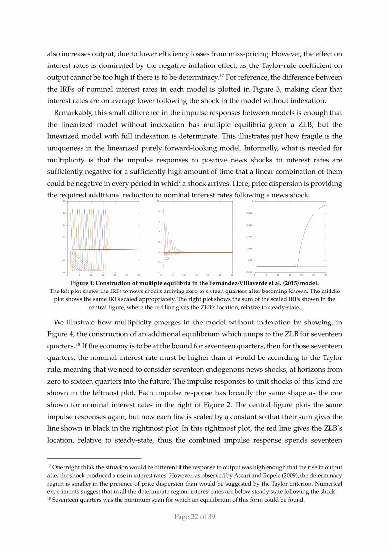
Figure 4: Construction of multiple equilibria in the Fernández-Villaverde et al. (2015) model.
The left plot shows the IRFs to news shocks arriving zero to sixteen quarters after becoming known. The middle plot shows the same IRFs scaled appropriately. The right plot shows the sum of the scaled IRFs shown in the
central figure, where the red line gives the ZLB’s location, relative to steady-state.
We illustrate how multiplicity emerges in the model without indexation by showing, in Figure 4, the construction of an additional equilibrium which jumps to the ZLB for seventeen quarters.18 If the economy is to be at the bound for seventeen quarters, then for those seventeen quarters, the nominal interest rate must be higher than it would be according to the Taylor rule, meaning that we need to consider seventeen endogenous news shocks, at horizons from zero to sixteen quarters into the future. The impulse responses to unit shocks of this kind are shown in the leftmost plot. Each impulse response has broadly the same shape as the one shown for nominal interest rates in the right of Figure 2. The central figure plots the same impulse responses again, but now each line is scaled by a constant so that their sum gives the line shown in black in the rightmost plot. In this rightmost plot, the red line gives the ZLB’s location, relative to steady-state, thus the combined impulse response spends seventeen
17 One might think the situation would be different if the response to output was high enough that the rise in output after the shock produced a rise in interest rates. However, as observed by Ascari and Ropele (2009), the determinacy region is smaller in the presence of price dispersion than would be suggested by the Taylor criterion. Numerical experiments suggest that in all the determinate region, interest rates are below steady-state following the shock. 18 Seventeen quarters was the minimum span for which an equilibrium of this form could be found.
0 5 10 15 20 25 30-0.4
-0.2
0
0.2
0.4
0.6
0.8
0 5 10 15 20 25 30-4
-2
0
2
4
6
8
10
0 5 10 15 20 25 30-0.012
-0.01
-0.008
-0.006
-0.004
-0.002
0

Page 23 of 39
quarters at the ZLB before returning to steady-state. Since there are only “news shocks” in the periods in which the economy is at the ZLB, this gives a perfect foresight rational expectations equilibrium which makes a self-fulfilling jump to the ZLB.
The situation is quite different under price level targeting. In particular, if we replace inflation in the monetary rule with the price level relative to its linear trend, which evolves according to:
𝑥𝑥𝑝𝑝,𝑡𝑡 = 𝑥𝑥𝑝𝑝,𝑡𝑡−1 + 𝑥𝑥𝜋𝜋,𝑡𝑡 − 𝑥𝑥𝜋𝜋, (5) then with 𝑇𝑇 = 200, the lower bound from Proposition 6 implies that 𝜍𝜍 > 0.003, and hence that for all sufficiently large 𝑇𝑇 , 𝑀𝑀 is an S-matrix (by Corollary 3), so there is always a feasible solution. Furthermore, even with 𝑇𝑇 = 1000, 𝑀𝑀 is a P-matrix by our sufficient conditions from Corollary 2. This is strongly suggestive of uniqueness even for arbitrarily large 𝑇𝑇, given the reasonably short-lived dynamics of the model.
5.3. The Smets & Wouters (2003; 2007) models Smets & Wouters (2003) and Smets & Wouters (2007) are the canonical medium-scale linear
DSGE models, featuring assorted shocks, habits, price and wage indexation, capital (with adjustment costs), (costly) variable utilisation and general monetary policy reaction functions. The former model is estimated on Euro area data, while the latter is estimated on US data. The latter model also contains trend growth (permitting its estimation on non-detrended data), and a slightly more general aggregator across industries. However, overall, they are quite similar models, and any differences in their behaviour chiefly stems from differences in the estimated parameters. Since both models are incredibly well known in the literature, we omit their equations here, referring the reader to the original papers for further details.
To assess the likelihood of multiple equilibria at or away from the zero lower bound, we augment each model with a ZLB on nominal interest rates, and evaluate the properties of each model’s 𝑀𝑀 matrix at the estimated posterior-modes from the original papers. To minimise the deviation from the original papers, we do not introduce an auxiliary variable for shadow nominal interest rates, so the monetary rules take the form of 𝑥𝑥𝑟𝑟,𝑡𝑡 = max�0, �1 − 𝜌𝜌𝑟𝑟�(⋯ ) +𝜌𝜌𝑟𝑟𝑥𝑥𝑟𝑟,𝑡𝑡−1 + ⋯ �, in both cases. Our results would be essentially identical with a shadow nominal interest rate though.
If the diagonal of the 𝑀𝑀 matrix ever goes negative, then the 𝑀𝑀 matrix cannot be semi-monotone, or P0, and hence the model will sometimes have multiple solutions even when away from the zero lower bound (i.e. for some positive 𝑞𝑞), by Proposition 4. In Figure 5, we plot the diagonal of the 𝑀𝑀 matrix for each model in turn,19 i.e. the impact on nominal interest rates in period 𝑡𝑡 of news in period 1 that a positive, magnitude one shock will hit nominal interest rates in period 𝑡𝑡 . Immediately, we see that while in the US model, these impacts remain positive at all horizons, in the Euro area model, these impacts turn negative after just a few
19 The MOD files for the Smets & Wouters (2003) and (2007) models were derived, respectively, from the Macro Model Database (Wieland et al. 2012) and files provided by Johannes Pfeifer here: http://goo.gl/CP53x5.

Page 24 of 39
periods, and remain so at least up to period 40. Therefore, in the ZLB augmented Smets & Wouters (2003) model, there is not always a unique equilibrium. Furthermore, if a run of future shocks was drawn from a distribution with unbounded support, then the value of these shocks was revealed to the model’s agents (as in the stochastic extended path), then there would be a positive probability that the model without the ZLB would always feature positive interest rates, but that the model with the ZLB could hit zero.
The Smets & Wouters (2003) model
The Smets & Wouters (2007) model
Figure 5: The diagonals of the 𝑴𝑴 matrices for the Smets & Wouters (2003; 2007) models
It remains for us to assess whether 𝑀𝑀 is a P(0)-matrix or (strictly) semi-monotone for the Smets & Wouters (2007) model. Numerical calculations reveal that for 𝑇𝑇 < 9, 𝑀𝑀 is a P-matrix, and hence is strictly semi-monotone. However, with 𝑇𝑇 ≥ 9, the top-left 9 × 9 sub-matrix of 𝑀𝑀 has negative determinant and is not an S or S(0) matrix. Thus, for 𝑇𝑇 ≥ 9, 𝑀𝑀 is not a P(0)-matrix or (strictly) semi-monotone, and hence this model also has multiple equilibria, even when away from the bound. While placing a larger coefficient on inflation in the Taylor rule can make the Euro area picture more like the US one, with a positive diagonal to the 𝑀𝑀 matrix, even with incredibly large coefficients, 𝑀𝑀 remains a non-P-matrix for both models. This is driven by the fact that both the real and nominal rigidities in the model help reduce the average value of the impulse response to a positive news shock to the monetary rule. Following such a shock’s arrival, they help ensure that the fall in output is persistent. Prior to its arrival, consumption habits and capital or investment adjustment costs help produce a larger anticipatory recession. Hence, in both the Euro area and the US, we ought to take seriously the possibility that the existence of the ZLB produces non-uniqueness.
As an example of such non-uniqueness, in Figure 6 we plot two different solutions following the most likely combination of shocks to the Smets & Wouters (2007) model that would produce negative interest rates for a year in the absence of a ZLB.20 In both cases, the dotted line shows the response in the absence of the ZLB. Particularly notable is the flip in sign, since
20 We find the vector 𝑤𝑤 that minimises 𝑤𝑤′𝑤𝑤 subject to 𝑟𝑟 ̅+ 𝑍𝑍𝑤𝑤 ≤ 0 , where 𝑟𝑟 ̅ is the steady-state interest rate, and columns of 𝑍𝑍 give four periods of the impulse response of interest rates to a given shocks. This gives the following shock magnitudes: productivity, 3.56% ; risk premium, −2.70 %; government, −1.63 %; investment, −4.43 %; monetary, −2.81%; price mark-up, −3.19%; wage mark-up, −4.14%.
0 5 10 15 20 25 30 35 40-0.3
-0.2
-0.1
0
0.1
0.2
0.3
0.4
0.5
0.6
0 5 10 15 20 25 30 35 400.3
0.35
0.4
0.45
0.5
0.55
0.6
0.65
0.7
0.75
0.8
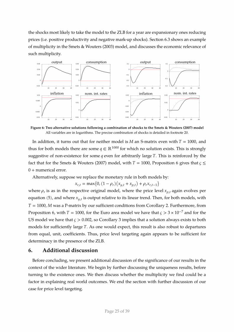
Page 25 of 39
the shocks most likely to take the model to the ZLB for a year are expansionary ones reducing prices (i.e. positive productivity and negative mark-up shocks). Section 6.3 shows an example of multiplicity in the Smets & Wouters (2003) model, and discusses the economic relevance of such multiplicity.
Figure 6: Two alternative solutions following a combination of shocks to the Smets & Wouters (2007) model
All variables are in logarithms. The precise combination of shocks is detailed in footnote 20.
In addition, it turns out that for neither model is 𝑀𝑀 an S-matrix even with 𝑇𝑇 = 1000, and thus for both models there are some 𝑞𝑞 ∈ ℝ1000 for which no solution exists. This is strongly suggestive of non-existence for some 𝑞𝑞 even for arbitrarily large 𝑇𝑇. This is reinforced by the fact that for the Smets & Wouters (2007) model, with 𝑇𝑇 = 1000, Proposition 6 gives that 𝜍𝜍 ≤0 + numerical error.
Alternatively, suppose we replace the monetary rule in both models by: 𝑥𝑥𝑟𝑟,𝑡𝑡 = max�0, �1 − 𝜌𝜌𝑟𝑟��𝑥𝑥𝑦𝑦,𝑡𝑡 + 𝑥𝑥𝑝𝑝,𝑡𝑡� + 𝜌𝜌𝑟𝑟𝑥𝑥𝑟𝑟,𝑡𝑡−1�
where 𝜌𝜌𝑟𝑟 is as in the respective original model, where the price level 𝑥𝑥𝑝𝑝,𝑡𝑡 again evolves per equation (5), and where 𝑥𝑥𝑦𝑦,𝑡𝑡 is output relative to its linear trend. Then, for both models, with
𝑇𝑇 = 1000, 𝑀𝑀 was a P-matrix by our sufficient conditions from Corollary 2. Furthermore, from Proposition 6, with 𝑇𝑇 = 1000, for the Euro area model we have that 𝜍𝜍 > 3 × 10⁻⁷ and for the US model we have that 𝜍𝜍 > 0.002, so Corollary 3 implies that a solution always exists to both models for sufficiently large 𝑇𝑇. As one would expect, this result is also robust to departures from equal, unit, coefficients. Thus, price level targeting again appears to be sufficient for determinacy in the presence of the ZLB.
6. Additional discussion
Before concluding, we present additional discussion of the significance of our results in the context of the wider literature. We begin by further discussing the uniqueness results, before turning to the existence ones. We then discuss whether the multiplicity we find could be a factor in explaining real world outcomes. We end the section with further discussion of our case for price level targeting.
10 20 30 40-0.02
0
0.02
0.04
0.06y_obs
10 20 30 40-0.02
0
0.02
0.04
0.06c_obs
10 20 30 40-0.01
-0.005
0
0.005
0.01pi_obs
10 20 30 40-0.01
0
0.01
0.02r_obs
10 20 30 40-0.3
-0.2
-0.1
0
0.1y_obs
10 20 30 40-0.2
-0.1
0
0.1c_obs
10 20 30 40-0.06
-0.04
-0.02
0
0.02pi_obs
10 20 30 40-0.01
0
0.01
0.02r_obs
output consumption
inflation nom. int. rates
output consumption
nom. int. rates inflation

Page 26 of 39
6.1. Uniqueness and multiplicity We have presented necessary and sufficient conditions for uniqueness in otherwise linear
models with terminal conditions. Some caveats are in order though. Bodenstein (2010) showed that linearization can exclude equilibria, and Braun, Körber &
Waki (2012) show that there may be multiple perfect-foresight solutions to a non-linear NK model with ZLB, converging to the non-deflationary steady-state. However, it turns out that the linearized version of their model has a unique equilibrium, even when the ZLB is imposed. Thus, the multiplicity we find is strictly in addition to the multiplicity found by those authors. While the theoretical and computational methods used by Braun, Körber & Waki (2012) have the great advantage that they can cope with fully non-linear models, it appears that they cannot cope with endogenous state variables, which limits their applicability. By producing tools for analysing otherwise linear models including state variables, our tools and results provide a complement to those of Braun, Körber & Waki (2012). For evidence of the continued relevance of our results in a non-linear setting, note that the multiplicity found in a simple linearized model in BPY (2013) is also found in the equivalent non-linear model in BPY (2016).
Of course, ideally, we would have liked to analyse models with other nonlinearities apart from the occasionally binding constraint(s). However, we maintain that studying multiplicity in otherwise linear models is still an important exercise. Firstly, macroeconomists have long relied on existence and uniqueness results based on linearization of models without occasionally binding constraints, even though this may produce spurious uniqueness in some circumstances. Secondly, it is nearly impossible to find all perfect foresight solutions in general non-linear models, since this is equivalent to finding all the solutions to a huge system of non-linear equations, when even finding all the solutions to large systems of quadratic equations is computationally intractable. At least if we have the full set of solutions to the otherwise linear model, we may use homotopy continuation methods to map these solutions into solutions of the non-linear model. Furthermore, finding all solutions under uncertainty is at least as difficult in general, as the policy function is also defined by a large system of non-linear equations. Thirdly, Christiano and Eichenbaum (2012) argue that e-learnability considerations render the additional equilibria of Braun, Körber & Waki (2012) mere “mathematical curiosities”, suggesting that the equilibria that exist in the linearized model are of independent interest, whatever one’s view on this debate. Finally, our main results for NK models imply non-uniqueness, so concerns of spurious uniqueness under linearization will not be relevant in these cases.
From the preceding discussion, we see that our choice to focus on otherwise-linear models under perfect-foresight, with fixed terminal conditions, has biased our results in favour of uniqueness for three distinct reasons. Firstly, because there are potentially more solutions under rational expectations than under perfect-foresight, as we prove in Appendix E, online; secondly, because there are potentially other solutions returning to alternate steady-states; and

Page 27 of 39
thirdly, because the original fully non-linear model may possess yet more solutions. This means our results on the multiplicity of solutions to New Keynesian models are all the more surprising, and that it is all the more likely that multiplicity of equilibria is an important factor in explaining actual economies’ spells at the ZLB.
Duarte (2016) considers how a central bank might ensure determinacy in a simple continuous time new Keynesian model. Like us, he finds that the Taylor principle is not sufficient in the presence of the ZLB. He shows that determinacy may be produced by using a rule that holds interest rates at zero for a history dependent amount of time, before switching to a max{0, … } Taylor rule. While we do not allow for such switches in central bank behaviour, we do find an important role for history dependence, through price targeting.
Jones (2015) also presents a uniqueness result for models with occasionally binding constraints. He shows that if one knows the set of periods at which the constraint binds, then under standard assumptions, there is a unique path. However, there is no reason there should be a unique set of periods at which the constraint binds, consistent with the model. The multiplicity for models with occasionally binding constraints precisely stems from there being multiple sets of periods at which the model could be at the bound. Our results are not conditional on knowing in advance the periods at which the constraint binds.
Finally, uniqueness results have also been derived in the Markov switching literature, see e.g. Davig & Leeper (2007) and Farmer, Waggoner & Zha (2010; 2011), though the assumed exogeneity of the switching in these papers limits their application to endogenous OBCs such as the ZLB. Determinacy results with endogenous switching were derived by Marx & Barthelemy (2013), but they only apply to forward looking models that are sufficiently close to ones with exogenous switching, and there is no reason e.g. a standard NK model with a ZLB should have this property. Our results do not have this limitation.
6.2. Existence and non-existence We also produced conditions for the existence of any perfect-foresight solution to an
otherwise linear model with a terminal condition. These results provide new intuition for the prior literature on existence under rational expectations, which has found that NK models with a ZLB might have no solution at all if the variance of shocks is too high. For example, Mendes (2011) derived analytic results on existence as a function of the variance of a demand shock, and Basu & Bundick (2015) showed the potential quantitative relevance of such results. Furthermore, conditions for the existence of an equilibrium in a simple NK model with discretionary monetary policy are derived in close form for a model with a two-state Markov shock by Nakata & Schmidt (2014). They show that the economy must spend a small amount of time in the bad state for the equilibrium to exist, which again links existence to variance.
While our results are not directly related to the variance of shocks, as we work under perfect foresight, they are nonetheless linked. We showed that whether a perfect foresight solution exists depends on the perfect-foresight path taken by nominal interest rates in the absence of

Page 28 of 39
the bound. Throughout, we assumed that this path was arbitrary, as there is always some information about future shocks that could be revealed today to produce a given path. However, in a model with a small number of shocks, all of bounded support, and no information about future shocks, clearly not all paths are possible for nominal interest rates in the absence of the bound. The more shocks are added (e.g. news shocks), and the wider their support, the greater will be the support of the space of possible paths for nominal interest rates in the absence of the ZLB, and hence, the more likely will be non-existence of a solution for a positive measure of paths, helping to explain the prior results.
There has also been some prior work by Richter & Throckmorton (2015) and Gavin et al. (2015; Appendix B) that has related a kind of eductive stability (the convergence of policy function iteration) to other properties of the model. Non-convergence of policy function iteration is suggestive of non-existence, though not definitive evidence. While the procedure of the cited authors has the advantage of working with the fully non-linear model under rational expectations, this limitation means that it cannot directly address the question of existence. By contrast, our results are theoretical and directly address existence. Thus, both procedures should be viewed as complementary; while ours definitively answers the question of existence in the slightly limited world of perfect foresight, otherwise linear models, the Richter & Throckmorton results give answers on stability in a richer setting.
Another approach to establishing the existence of an equilibrium is to produce it to satisfactory accuracy, by solving the model in some way. Under perfect foresight, the procedure outlined in this paper’s companion is a possibility (Holden 2016), and the method of Guerrieri & Iacoviello (2012) is a prominent alternative. Under rational expectations, policy function iteration methods have been used by Fernández-Villaverde et al. (2015) and Richter & Throckmorton (2015), amongst others. However, this approach cannot establish non-existence or prove uniqueness. As such it is of little use to the policy maker who wants policy guidance to ensure existence and/or uniqueness. Furthermore, if the problem is solved globally, one cannot in general rule out that there is not an area of non-existence outside of the grid on which the model was solved. Similarly, if the model is solved under perfect foresight for a given initial state, then the fact that a solution exists for that initial point gives no guarantees that a solution should exist for other initial points. Thus, there is an essential role for more general results on global existence, as we have produced here.
6.3. Economic significance of multiplicity at the ZLB There are two reasons why one might be sceptical about the economic significance of the
multiple equilibria caused by the presence of the ZLB that we find. Firstly, as with any non-fundamental equilibrium, the coordination of beliefs needed to sustain the equilibrium may be difficult. Secondly, as we have seen, self-fulfilling jumps to the ZLB may feature implausibly large falls in output and inflation. This reflects the implausibly large response to news about future policy innovations, a problem that has been termed the “forward guidance puzzle” in

Page 29 of 39
the literature (Carlstrom, Fuerst & Paustian 2015; Del Negro, Giannoni & Patterson 2015).21 However, if the economy is already in a recession, then both problems are substantially ameliorated. If interest rates are already low, then it does not seem too great a stretch to suggest that a drop in confidence may lead people to expect to hit the ZLB. Even more plausibly, if the economy is already at the ZLB, then small changes in confidence could easily select an equilibrium featuring a longer spell at the ZLB than in the equilibrium with the shortest time there. Indeed, there is no good reason people should coordinate on the equilibrium with the shortest time at the ZLB. Moreover, with interest rates already low, the size of the required self-fulfilling news shock is much smaller, meaning that the additional drop in output and inflation caused by a jump to the ZLB will be much more moderate.
Figure 7: Two solutions following a preference shock in the Smets & Wouters (2003) model.
All variables are in logarithms. The dotted line is a solution which does not hit the bound. The solid line is an alternative solution which does hit the bound.
As an illustration, in Figure 7 we plot the impulse response to a large magnitude preference shock (scaling utility), in the Smets & Wouters (2003) model.22 The shock is not quite large
21 McKay, Nakamura & Steinsson (2016) point out that these implausibly large responses to news are muted in models with heterogeneous agents, and give a simple “discounted Euler” approximation that produces similar results to a full heterogeneous agent model. While including a discounted Euler equation makes it harder to generate multiplicity (e.g. reducing the parameter space with multiplicity in the BPY (2013) model), when there is multiplicity, the resulting responses are much larger, as the weaker response to news means the required endogenous news shocks need to be much greater in order to drive the model to the bound. 22 The shock is 22.5 standard deviations. While this is implausibly large, the economy could be driven to the bound with a run of much smaller shocks. It is also worth recalling that the model was estimated on the great moderation period, and so the estimated standard deviations may be too low. Finally, recent evidence (Cúrdia, del Negro & Greenwald 2014) suggests that the shocks in DSGE models should be fat tailed, making large shocks more likely.
5 10 15 20 25 30 35 40-0.14
-0.12
-0.1
-0.08
-0.06
-0.04
-0.02
0
0.02
0.04yobs
5 10 15 20 25 30 35 40-0.25
-0.2
-0.15
-0.1
-0.05
0
0.05cobs
5 10 15 20 25 30 35 40-18
-16
-14
-12
-10
-8
-6
-4
-2
0
210 -3 piobs
5 10 15 20 25 30 35 40-0.005
0
0.005
0.01
0.015
0.02
0.025robs
output consumption
inflation nominal interest rates

Page 30 of 39
enough to send the economy to the ZLB23 in the standard solution, shown with a dotted line. However, there is an alternative solution in which the economy jumps to the bound one period after the initial shock, remaining there for three periods. While the alternative solution features larger drops in output and inflation, the falls are broadly in line with the magnitude of the crisis, with Eurozone GDP and consumption now being about 20% below a pre-crisis log-linear trend, and the largest drop in Eurozone consumption inflation from 2008q3 to 2008q4 being around 1%. 24 Considering this, we view it as plausible that multiplicity of equilibria was a significant component of the explanation for the great recession.
6.4. Price level targeting Our results suggest that given belief in an eventual return to inflation, a determinate
equilibrium may be produced in standard NK models if the central bank switches to targeting the price level, rather than the inflation rate. As the previous figure made clear, the welfare benefits to this could be substantial. There is of course a large literature advocating price level targeting already. Vestin (2006) made an important early contribution by showing that its history dependence mimics the optimal rule, a conclusion reinforced by Giannoni (2010). Eggertsson & Woodford (2003) showed the particular desirability of price level targeting in the presence of the ZLB, since it produces inflation after the bound is escaped. A later contribution by Nakov (2008) showed that this result survived taking a fully global solution, and Coibion, Gorodnichenko & Wieland (2012) showed that it still holds in a richer model. More recently, Basu & Bundick (2015) have argued that a response to the price level avoids the kinds of equilibrium non-existence problems stressed by Mendes (2011), while also solving the contractionary bias caused by the ZLB. Our argument is distinct from these; we showed that in the presence of the ZLB, inflation targeting rules are indeterminate, even conditional on an eventual return to inflation, whereas price level targeting rules produce determinacy, in the sense of the existence of a unique path returning to the inflationary steady state.
Our results are also distinct from those of Adão, Correia & Teles (2011) who showed that if the central bank is not constrained to respect the ZLB out of equilibrium, and if the central bank uses a rule that responds to the right hand side of the Euler equation, then a globally unique equilibrium may be produced, even without ruling out explosive beliefs about prices. Their rule has the flavour of a (future) price-targeting rule, due to the presence of future prices in the right-hand side of the Euler equation. Here though, we are assuming that the central bank must satisfy the ZLB even out of equilibrium, which makes it harder to produce
23 Since the Smets & Wouters (2003) model does not include trend growth, it is impossible to produce a steady-state value for nominal interest rates that is consistent with both the model and the data. We choose to follow the data, setting the steady-state of nominal interest rates to its mean level over the same sample period used by Smets & Wouters (2003), using data from the same source (Fagan, Henry & Mestre 2005). 24 Data was again from the area-wide model database (Fagan, Henry & Mestre 2005).

Page 31 of 39
uniqueness. Additionally, we do not require that the central bank can choose a knife-edge value for its response to the (future) price-level, or that it knows the precise form of agents’ utility functions, both of which are apparently required by the rule of Adão, Correia & Teles and which may be difficult in practice. However, in line with the New Keynesian literature, we maintain the standard assumption that explosive paths for inflation are ruled out, an assumption which the knife-edge rules of Adão, Correia & Teles do not require.25
Somewhat contrary to our results, Armenter (2016) shows that in a simple otherwise linear NK model, if the central bank pursues Markov (discretionary) policy subject to an objective targeting inflation, nominal GDP or the price level, then the presence of a ZLB produces additional equilibria quite generally. This difference between our results and those of Armenter (2016) is driven both by the fact that we rule out getting stuck in the neighbourhood of the deflationary steady-state by assumption, and since we assume commitment to a rule.
7. Conclusion
This paper provides the first general theoretical results on existence and uniqueness for otherwise linear models with occasionally binding constraints, given terminal conditions. As such, it may be viewed as doing for models with occasionally binding constraints what Blanchard & Kahn (1980) did for linear models.
We provided necessary and sufficient conditions for the existence of a unique equilibrium, as well as such conditions for uniqueness when away from the bound, all conditional on the economy returning to a specific steady-state. We also provide a toolkit (“DynareOBC”) which verifies these conditions. In our application to New Keynesian models, we showed that these conditions were violated in entirely standard models, rather than just being a consequence of policy rules responding to growth rates. In the presence of multiplicity, there is the potential for additional endogenous volatility from sunspots, so the welfare benefits of avoiding multiplicity may be substantial. Moreover, we saw that the additional equilibria may feature huge drops in output, providing further reasons for their avoidance.
Luckily, our results give policy makers a solution. Providing agents believe in an eventual return to inflation, pursuing a price level targeting rule will produce a determinate equilibrium in standard NK models, even in the presence of the ZLB. Consequently, if one believes the arguments for the Taylor principle in the absence of the ZLB, then one should advocate price level targeting if the ZLB constraint is inescapable.
In addition, we provided conditions for existence of any solution that converges to the “good” steady-state, conditions which again may be verified using our DynareOBC toolkit. We showed that under inflation targeting, standard NK models again failed to satisfy these conditions over all the space of state variables and shocks. Whereas the literature started by
25 Note that the unstable solutions under price level targeting feature exponential growth in the logarithm of the price level, which also implies explosions in inflation rates.

Page 32 of 39
Benhabib, Schmitt-Grohé & Uribe (2001a; 2001b) showed that the existence of a “bad” steady-state may imply additional volatility if agents long-run beliefs are not pinned down by the inflation target, here we showed that under inflation targeting, there was positive probability of arriving in a state from which there was no way for the economy to converge to the “good” steady-state. This in turn implies that agents should not place prior certainty on converging to the “good” steady-state, thus rationalising the beliefs required to get the kind of global multiplicity at the zero lower bound that these and other authors have focussed on.
: Generalizations
It is straightforward to generalise the results of this paper to less restrictive otherwise linear models with occasionally binding constraints.
Firstly, if the constraint is on a variable other than 𝑥𝑥1,𝑡𝑡, or in another equation than the first, then all of the results go through as before, just by relabelling and rearranging. Furthermore, if the constraint takes the form of 𝑧𝑧1,𝑡𝑡 = max�𝑧𝑧2,𝑡𝑡, 𝑧𝑧3,𝑡𝑡� , where 𝑧𝑧1,𝑡𝑡 , 𝑧𝑧2,𝑡𝑡 and 𝑧𝑧3,𝑡𝑡 are linear expressions in the contemporaneous values, lags and leads of 𝑥𝑥𝑡𝑡, then, assuming without loss of generality that 𝑧𝑧3,⋅ > 𝑧𝑧2,⋅ in steady-state, we have that 𝑧𝑧1,𝑡𝑡 − 𝑧𝑧2,𝑡𝑡 = max�0, 𝑧𝑧3,𝑡𝑡 − 𝑧𝑧2,𝑡𝑡�. Hence, adding a new auxiliary variable 𝑥𝑥𝑛𝑛+1,𝑡𝑡, with the associated equation 𝑥𝑥𝑛𝑛+1,𝑡𝑡 = 𝑧𝑧1,𝑡𝑡 − 𝑧𝑧2,𝑡𝑡, and replacing the constrained equation with 𝑥𝑥𝑛𝑛+1,𝑡𝑡 = max�0, 𝑧𝑧3,𝑡𝑡 − 𝑧𝑧2,𝑡𝑡�, we have a new equation in the form covered by our results. Moreover, if rather than a max we have a min, we just use the fact that if 𝑧𝑧1,𝑡𝑡 = min�𝑧𝑧2,𝑡𝑡, 𝑧𝑧3,𝑡𝑡� , then −𝑧𝑧1,𝑡𝑡 = max�−𝑧𝑧2,𝑡𝑡, −𝑧𝑧3,𝑡𝑡� , which is covered by the generalisation just established. The easiest encoding of the complementary slackness conditions, 𝑧𝑧𝑡𝑡 ≥ 0, 𝜆𝜆𝑡𝑡 ≥ 0 and 𝑧𝑧𝑡𝑡𝜆𝜆𝑡𝑡 = 0, is 0 = min{𝑧𝑧𝑡𝑡, 𝜆𝜆𝑡𝑡}, which is of this form.
To deal with multiple occasionally binding constraints, we use the representation from Holden and Paetz (2012). Suppose there are 𝑐𝑐 constrained variables in the model. For 𝑎𝑎 ∈{1, … , 𝑐𝑐}, let 𝑞𝑞(𝑎𝑎) be the path of the 𝑎𝑎th constrained variable in the absence of all constraints. For 𝑎𝑎, 𝑏𝑏 ∈ {1, … , 𝑐𝑐} , let 𝑀𝑀(𝑎𝑎,𝑏𝑏) be the matrix created by horizontally stacking the column vector relative impulse responses of the 𝑎𝑎 th constrained variable to magnitude 1 news shocks at horizon 0, … , 𝑇𝑇 − 1 to the equation defining the 𝑏𝑏th constrained variables. For example, if 𝑐𝑐 =1 so there is a single constraint, then we would have that 𝑀𝑀(1,1) = 𝑀𝑀 as defined in equation (2). Finally, let:
𝑞𝑞 ≔⎣⎢⎢⎡𝑞𝑞(1)
⋮𝑞𝑞(𝑐𝑐)⎦
⎥⎥⎤ , 𝑀𝑀 ≔
⎣⎢⎡
𝑀𝑀(1,1) ⋯ 𝑀𝑀(1,𝑐𝑐)
⋮ ⋱ ⋮𝑀𝑀(𝑐𝑐,1) ⋯ 𝑀𝑀(𝑐𝑐,𝑐𝑐)⎦
⎥⎤,
and let 𝑦𝑦 be a solution to the LCP �𝑞𝑞, 𝑀𝑀�. Then the vertically stacked paths of the constrained variables in a solution which satisfies these constraints is given by 𝑞𝑞 + 𝑀𝑀𝑦𝑦, and Theorem 1 goes through as before.

Page 33 of 39
: Additional matrix properties and their relationships
Definition 7 ((Non-)Degenerate matrix) A matrix 𝑀𝑀 ∈ ℝ𝑇𝑇×𝑇𝑇 is called a non-degenerate matrix if the principal minors of 𝑀𝑀 are all non-zero. 𝑀𝑀 is called a degenerate matrix if it is not a non-degenerate matrix.
Definition 8 (Sufficient matrices) Let 𝑀𝑀 ∈ ℝ𝑇𝑇×𝑇𝑇. 𝑀𝑀 is called column sufficient if 𝑀𝑀 is a P0-matrix, and for each principal sub-matrix 𝑊𝑊 ≔ �𝑀𝑀𝑖𝑖,𝑗𝑗�𝑖𝑖,𝑗𝑗=𝑘𝑘1,…,𝑘𝑘𝑆𝑆
of 𝑀𝑀, with zero determinant,
and for each proper principal sub-matrix �𝑊𝑊𝑖𝑖,𝑗𝑗�𝑖𝑖,𝑗𝑗=𝑙𝑙1,…,𝑙𝑙𝑅𝑅 of 𝑊𝑊 (𝑅𝑅 < 𝑆𝑆), with zero determinant,
the columns of �𝑊𝑊𝑖𝑖,𝑗𝑗� 𝑖𝑖=1,…,𝑆𝑆𝑗𝑗=𝑙𝑙1,…,𝑙𝑙𝑅𝑅
do not form a basis for the column space of 𝑊𝑊.26 𝑀𝑀 is called row
sufficient if 𝑀𝑀′ is column sufficient. 𝑀𝑀 is called sufficient if it is column sufficient and row sufficient.
Definition 9 ((Strictly) Copositive) A matrix 𝑀𝑀 ∈ ℝ𝑇𝑇×𝑇𝑇 is called (strictly) copositive if 𝑀𝑀 +𝑀𝑀′ is (strictly) semi-monotone.27
Cottle, Pang & Stone (2009a) note the following relationships between these classes (amongst others):
Lemma 4 The following hold: 1) All general positive semi-definite matrices are copositive and sufficient. 2) P0 includes skew-symmetric, general p.s.d., sufficient and P matrices. 3) All P0-matrices, and all copositive matrices are semi-monotone, and all P-matrices, and all
strictly copositive matrices are strictly semi-monotone.
: Other properties of the solution set
Conditions for having a finite or convex set of solutions are given in the following propositions:
Proposition 11 The LCP �𝑞𝑞, 𝑀𝑀� has a finite (possibly zero) number of solutions for all 𝑞𝑞 ∈ ℝ𝑇𝑇 if and only if 𝑀𝑀 is non-degenerate. (Cottle, Pang & Stone 2009a)
Proposition 12 The LCP �𝑞𝑞, 𝑀𝑀� has a convex (possibly empty) set of solutions for all 𝑞𝑞 ∈ ℝ𝑇𝑇 if and only if 𝑀𝑀 is column sufficient. (Cottle, Pang & Stone 2009a)
: Results from dynamic programming
Alternative existence and uniqueness results for the infinite 𝑇𝑇 problem can be established via dynamic programming methods, under the assumption that Problem 2 (OBC) comes from the first order conditions solution of a social planner problem. These have the advantage that
26 This may be checked via the singular value decomposition. 27 Väliaho (1986) contains an alternative characterisation which avoids solving any linear programming problems.

Page 34 of 39
their conditions are potentially much easier to evaluate, though they also have somewhat limited applicability. We focus here on uniqueness results, since these are of greater interest.
Suppose that the social planner in some economy solves the following problem:
Problem 5 (Linear-Quadratic) Suppose 𝜇𝜇 ∈ ℝ𝑛𝑛 , Ψ(0) ∈ ℝ𝑐𝑐×1 and Ψ(1) ∈ ℝ𝑐𝑐×2𝑛𝑛 are given, where 𝑐𝑐 ∈ ℕ. Define Γ̃: ℝ𝑛𝑛 → ℙ(ℝ𝑛𝑛) (where ℙ denotes the power-set operator) by:
Γ̃(𝑥𝑥) = �𝑧𝑧 ∈ ℝ𝑛𝑛�0 ≤ Ψ(0) + Ψ(1) �𝑥𝑥 − 𝜇𝜇𝑧𝑧 − 𝜇𝜇�� , (6)
for all 𝑥𝑥 ∈ ℝ𝑛𝑛. (Note: 𝛤𝛤̃(𝑥𝑥) will give the set of feasible values for next period’s state if the current state is 𝑥𝑥. Equality constraints may be included by including an identical lower bound and upper bound.) Define:
𝑋𝑋� ≔ �𝑥𝑥 ∈ ℝ𝑛𝑛�Γ̃(𝑥𝑥) ≠ ∅�, (7) and suppose without loss of generality that for all 𝑥𝑥 ∈ ℝ𝑛𝑛, Γ̃(𝑥𝑥) ∩ 𝑋𝑋� = Γ̃(𝑥𝑥). (Note: this means that the linear inequalities bounding 𝑋𝑋� are already included in those in the definition of 𝛤𝛤̃(𝑥𝑥). It is without loss of generality as the planner will never choose an 𝑥𝑥̃ ∈ 𝛤𝛤̃(𝑥𝑥) such that 𝛤𝛤̃(𝑥𝑥)̃ = ∅.) Further define ℱ̃ : 𝑋𝑋� × 𝑋𝑋� → ℝ by:
ℱ̃(𝑥𝑥, 𝑧𝑧) = 𝑢𝑢(0) + 𝑢𝑢(1) �𝑥𝑥 − 𝜇𝜇𝑧𝑧 − 𝜇𝜇� +
12 �
𝑥𝑥 − 𝜇𝜇𝑧𝑧 − 𝜇𝜇�
′𝑢𝑢(̃2) �
𝑥𝑥 − 𝜇𝜇𝑧𝑧 − 𝜇𝜇� , (8)
for all 𝑥𝑥, 𝑧𝑧 ∈ 𝑋𝑋� , where 𝑢𝑢(0) ∈ ℝ , 𝑢𝑢(1) ∈ ℝ1×2𝑛𝑛 and 𝑢𝑢(̃2) = 𝑢𝑢(̃2)′ ∈ ℝ2𝑛𝑛×2𝑛𝑛 are given. Finally, suppose 𝑥𝑥0 ∈ 𝑋𝑋� is given and 𝛽𝛽 ∈ (0,1), and choose 𝑥𝑥1, 𝑥𝑥2, … to maximise:
lim inf𝑇𝑇→∞
� 𝛽𝛽𝑡𝑡−1ℱ̃(𝑥𝑥𝑡𝑡−1, 𝑥𝑥𝑡𝑡)𝑇𝑇
𝑡𝑡=1(9)
subject to the constraints that for all 𝑡𝑡 ∈ ℕ+, 𝑥𝑥𝑡𝑡 ∈ Γ̃(𝑥𝑥𝑡𝑡−1).
To ensure the problem is well behaved, we make the following assumption:
Assumption 4 𝑢𝑢(̃2) is negative-definite.
In Appendix H.10, online, we establish the following (unsurprising) result:
Proposition 13 If either 𝑋𝑋� is compact, or, Γ̃(𝑥𝑥) is compact valued and 𝑥𝑥 ∈ Γ̃(𝑥𝑥) for all 𝑥𝑥 ∈ 𝑋𝑋�, then for all 𝑥𝑥0 ∈ 𝑋𝑋�, there is a unique path (𝑥𝑥𝑡𝑡)𝑡𝑡=0
∞ which solves Problem 5 (Linear-Quadratic).
We wish to use this result to establish the uniqueness of the solution to the first order conditions. The Lagrangian for our problem is given by:
� 𝛽𝛽𝑡𝑡−1
⎣⎢⎡ℱ̃(𝑥𝑥𝑡𝑡−1, 𝑥𝑥𝑡𝑡) + 𝜆𝜆Ψ,𝑡𝑡
′ �Ψ(0) + Ψ(1) �𝑥𝑥𝑡𝑡−1 − 𝜇𝜇𝑥𝑥𝑡𝑡 − 𝜇𝜇 ��
⎦⎥⎤
∞
𝑡𝑡=1, (10)
for some KKT-multipliers 𝜆𝜆𝑡𝑡 ∈ ℝ𝑐𝑐 for all 𝑡𝑡 ∈ ℕ+. Taking the first order conditions leads to the following necessary KKT conditions, for all 𝑡𝑡 ∈ ℕ+:
0 = 𝑢𝑢⋅,2(1) + �
𝑥𝑥𝑡𝑡−1 − 𝜇𝜇𝑥𝑥𝑡𝑡 − 𝜇𝜇 �
′𝑢𝑢⋅̃,2
(2) + 𝜆𝜆𝑡𝑡′Ψ⋅,2
(1) + 𝛽𝛽 �𝑢𝑢⋅,1(1) + �
𝑥𝑥𝑡𝑡 − 𝜇𝜇𝑥𝑥𝑡𝑡+1 − 𝜇𝜇�
′𝑢𝑢⋅̃,1
(2) + 𝜆𝜆𝑡𝑡+1′ Ψ⋅,1
(1)� , (11)
0 ≤ Ψ(0) + Ψ(1) �𝑥𝑥𝑡𝑡−1 − 𝜇𝜇𝑥𝑥𝑡𝑡 − 𝜇𝜇 � , 0 ≤ 𝜆𝜆𝑡𝑡, 0 = 𝜆𝜆𝑡𝑡 ∘ �Ψ(0) + Ψ(1) �
𝑥𝑥𝑡𝑡−1 − 𝜇𝜇𝑥𝑥𝑡𝑡 − 𝜇𝜇 �� , (12)
where subscripts 1 and 2 refer to blocks of rows or columns of length 𝑛𝑛. Additionally, for 𝜇𝜇 to be the steady-state of 𝑥𝑥𝑡𝑡 and 𝜆𝜆���� to be the steady-state of 𝜆𝜆𝑡𝑡, we require:

Page 35 of 39
0 = 𝑢𝑢⋅,2(1) + 𝜆𝜆���� ′Ψ⋅,2
(1) + 𝛽𝛽�𝑢𝑢⋅,1(1) + 𝜆𝜆����′Ψ⋅,1
(1)�, (13)
0 ≤ Ψ(0), 0 ≤ 𝜆𝜆����, 0 = 𝜆𝜆���� ∘ Ψ(0). (14) In Appendix H.11, online, we prove the following result:
Proposition 14 Suppose that for all 𝑡𝑡 ∈ ℕ, (𝑥𝑥𝑡𝑡)𝑡𝑡=1∞ and (𝜆𝜆𝑡𝑡)𝑡𝑡=1
∞ satisfy the KKT conditions given in equations (11) and (12) , and that as 𝑡𝑡 → ∞ , 𝑥𝑥𝑡𝑡 → 𝜇𝜇 and 𝜆𝜆𝑡𝑡 → 𝜆𝜆���� , where 𝜇𝜇 and 𝜆𝜆 satisfy the steady-state KKT conditions given in equations (13) and (14). Then (𝑥𝑥𝑡𝑡)𝑡𝑡=1
∞ solves Problem 5 (Linear-Quadratic). If, further, either condition of Proposition 13 is satisfied, then (𝑥𝑥𝑡𝑡)𝑡𝑡=1
∞ is the unique solution to Problem 5 (Linear-Quadratic), and there can be no other solutions to the KKT conditions given in equations (11) and (12) satisfying 𝑥𝑥𝑡𝑡 → 𝜇𝜇 and 𝜆𝜆𝑡𝑡 → 𝜆𝜆���� as 𝑡𝑡 → ∞.
Now, it is possible to convert the KKT conditions given in equations (11) and (12) into a problem in the form of the multiple-bound generalisation of Problem 2 (OBC) quite generally. To see this, first note that we may rewrite equation (11) as:
0 = 𝑢𝑢⋅,2(1)′
+ 𝑢𝑢2̃,1(2)�𝑥𝑥𝑡𝑡−1 − 𝜇𝜇� + 𝑢𝑢2̃,2
(2)�𝑥𝑥𝑡𝑡 − 𝜇𝜇� + Ψ⋅,2(1)′
𝜆𝜆𝑡𝑡
+ 𝛽𝛽�𝑢𝑢⋅,1(1)′
+ 𝑢𝑢1̃,1(2)�𝑥𝑥𝑡𝑡 − 𝜇𝜇� + 𝑢𝑢1̃,2
(2)�𝑥𝑥𝑡𝑡+1 − 𝜇𝜇� + Ψ⋅,1(1)′
𝜆𝜆𝑡𝑡+1�.
Now, 𝑢𝑢2̃,2(2) + 𝛽𝛽𝑢𝑢1,1
(2) is negative definite, hence we may define 𝒱𝒱 ≔ Ψ⋅,2(1)�𝑢𝑢2̃,2
(2) + 𝛽𝛽𝑢𝑢1̃,1(2)�
−1, so:
Ψ(0) + Ψ(1) �𝑥𝑥𝑡𝑡−1 − 𝜇𝜇𝑥𝑥𝑡𝑡 − 𝜇𝜇 �
= Ψ(0) + �Ψ⋅,1(1) − 𝒱𝒱𝑢𝑢2̃,1
(2)��𝑥𝑥𝑡𝑡−1 − 𝜇𝜇� − 𝒱𝒱 �𝑢𝑢⋅,2(1)′
+ 𝛽𝛽�𝑢𝑢⋅,1(1)′
+ 𝑢𝑢1̃,2(2)�𝑥𝑥𝑡𝑡+1 − 𝜇𝜇� + Ψ⋅,1
(1)′𝜆𝜆𝑡𝑡+1��
−Ψ⋅,2(1)�𝑢𝑢2̃,2
(2) + 𝛽𝛽𝑢𝑢1̃,1(2)�
−1Ψ⋅,2
(1)′𝜆𝜆𝑡𝑡.
(15)
Moreover, equation (12) implies that if the 𝑘𝑘 th element of Ψ(0) + Ψ(1) �𝑥𝑥𝑡𝑡−1 − 𝜇𝜇𝑥𝑥𝑡𝑡 − 𝜇𝜇 � is positive,
then the 𝑘𝑘th element of 𝜆𝜆𝑡𝑡 is zero, so: Ψ(0) + Ψ(1) �
𝑥𝑥𝑡𝑡−1 − 𝜇𝜇𝑥𝑥𝑡𝑡 − 𝜇𝜇 � = max{0, 𝑧𝑧𝑡𝑡} , (16)
where: 𝑧𝑧𝑡𝑡 ≔ Ψ(0) + �Ψ⋅,1
(1) − 𝒱𝒱𝑢𝑢2̃,1(2)��𝑥𝑥𝑡𝑡−1 − 𝜇𝜇� − 𝒱𝒱 �𝑢𝑢⋅,2
(1)′+ 𝛽𝛽�𝑢𝑢⋅,1
(1)′+ 𝑢𝑢1̃,2
(2)�𝑥𝑥𝑡𝑡+1 − 𝜇𝜇� + Ψ⋅,1(1)′
𝜆𝜆𝑡𝑡+1��
− �Ψ⋅,2(1)�𝑢𝑢2̃,2
(2) + 𝛽𝛽𝑢𝑢1̃,1(2)�
−1Ψ⋅,2
(1)′+ 𝒲𝒲� 𝜆𝜆𝑡𝑡,
and 𝒲𝒲 ∈ ℝ𝑐𝑐×𝑐𝑐 is an arbitrary, positive diagonal matrix. A natural choice is: 𝒲𝒲 ≔ − diag−1 diag �Ψ⋅,2
(1)�𝑢𝑢2̃,2(2) + 𝛽𝛽𝑢𝑢1̃,1
(2)�−1
Ψ⋅,2(1)′
�,
providing this is positive (it is nonnegative at least as 𝑢𝑢2̃,2(2) + 𝛽𝛽𝑢𝑢1̃,1
(2) is negative definite), where
the diag operator maps matrices to a vector containing their diagonal, and diag−1 maps vectors to a matrix with the given vector on the diagonal, and zeros elsewhere.
We claim that we may replace equation (12) with equation (16) without changing the model. We have already shown that equation (12) implies equation (16), so we just have to prove the converse. We continue to suppose equation (11) holds, and thus, so too does equation (15). Then, from subtracting equation (15) from equation (16), we have that:
𝒲𝒲𝜆𝜆𝑡𝑡 = max{−𝑧𝑧𝑡𝑡, 0}.

Page 36 of 39
Hence, as 𝒲𝒲 is a positive diagonal matrix, and the right-hand side is nonnegative, 𝜆𝜆𝑡𝑡 ≥ 0 . Furthermore, the 𝑘𝑘th element of 𝜆𝜆𝑡𝑡 is non-negative if and only if the 𝑘𝑘th element of 𝑧𝑧𝑡𝑡 is non-positive (as 𝒲𝒲 is a positive diagonal matrix), which in turn holds if and only if the 𝑘𝑘th element of Ψ(0) + Ψ(1) �
𝑥𝑥𝑡𝑡−1 − 𝜇𝜇𝑥𝑥𝑡𝑡 − 𝜇𝜇 � is equal to zero, by equation (16). Thus equation (12) is satisfied.
Combined with our previous results, this gives the following proposition:
Proposition 15 Suppose we are given a problem in the form of Problem 5 (Linear-Quadratic). Then, the KKT conditions of that problem may be placed into the form of the multiple-bound generalisation of Problem 2 (OBC). Let �𝑞𝑞𝑥𝑥0
, 𝑀𝑀� be the infinite LCP corresponding to this representation, given initial state 𝑥𝑥0 ∈ 𝑋𝑋�. Then, if 𝑦𝑦 is a solution to the LCP, 𝑞𝑞𝑥𝑥0
+ 𝑀𝑀𝑦𝑦 gives the
stacked paths of the bounded variables in a solution to Problem 5 (Linear-Quadratic). If, further, either condition of Proposition 13 is satisfied, then this LCP has a unique solution for all 𝑥𝑥0 ∈ 𝑋𝑋� , which gives the unique solution to Problem 5 (Linear-Quadratic), and, for sufficiently large 𝑇𝑇∗ , the finite LCP �𝑞𝑞𝑥𝑥0
(𝑇𝑇∗), 𝑀𝑀(𝑇𝑇∗)� has a unique solution 𝑦𝑦(𝑇𝑇∗) for all 𝑥𝑥0 ∈ 𝑋𝑋� , where 𝑞𝑞𝑥𝑥0
(𝑇𝑇∗) + 𝑀𝑀(𝑇𝑇∗)𝑦𝑦(𝑇𝑇∗) gives the first 𝑇𝑇∗ periods of the stacked paths of the bounded
variables in a solution to Problem 5 (Linear-Quadratic).
This proposition provides some evidence that the LCP will have a unique solution when it is generated from a dynamic programming problem with a unique solution. In Appendix F, online, we derive similar results for models with more general constraints and objective functions. The proof of this proposition also showed an alternative method for converting KKT conditions into equations of the form handled by our methods.
References Adão, Bernardino, Isabel Correia & Pedro Teles. 2011. ‘Unique Monetary Equilibria with Interest Rate
Rules’. Review of Economic Dynamics 14 (3) (July): 432–442. Adjemian, Stéphane & Michel Juillard. 2013. ‘Stochastic Extended Path Approach’. ———. 2016. ‘The Stochastic Extended Path Approach’. National Bank of Belgium. Aliprantis, C.D. & K. Border. 2013. Infinite Dimensional Analysis: A Hitchhiker’s Guide. Studies in
Economic Theory. Springer Berlin Heidelberg. Anderson, Gary. 2015. ‘A Solution Strategy for Occasionally Binding Constraints’. Unpublished. Armenter, Roc. 2016. The Perils of Nominal Targets. Federal Reserve Bank of Philadelphia. Aruoba, S. Borağan, Pablo Cuba-Borda & Frank Schorfheide. 2014. Macroeconomic Dynamics Near the
ZLB: A Tale of Two Countries. Penn Institute for Economic Research, Department of Economics, University of Pennsylvania.
Ascari, Guido & Tiziano Ropele. 2009. ‘Trend Inflation, Taylor Principle, and Indeterminacy’. Journal of Money, Credit and Banking 41 (8). Journal of Money, Credit and Banking: 1557–1584.
Bai, Zhong-Zhi & D.J. Evans. 1997. ‘Matrix Multisplitting Relaxation Methods for Linear Complementarity Problems’. International Journal of Computer Mathematics 63 (3–4) (January 1): 309–326.
Basu, Susanto & Brent Bundick. 2015. ‘Endogenous Volatility at the Zero Lower Bound: Implications for Stabilization Policy’. National Bureau of Economic Research Working Paper Series No. 21838.
Beaudry, Paul & Franck Portier. 2006. ‘Stock Prices, News, and Economic Fluctuations’. American Economic Review 96 (4): 1293–1307.

Page 37 of 39
Benhabib, Jess, Stephanie Schmitt-Grohé & Martín Uribe. 2001a. ‘Monetary Policy and Multiple Equilibria’. American Economic Review 91 (1). American Economic Review: 167–186.
———. 2001b. ‘The Perils of Taylor Rules’. Journal of Economic Theory 96 (1–2). Journal of Economic Theory: 40–69.
Benigno, Pierpaolo & Michael Woodford. 2012. ‘Linear-Quadratic Approximation of Optimal Policy Problems’. Journal of Economic Theory 147 (1). Journal of Economic Theory: 1–42.
Blanchard, Olivier Jean & Charles M. Kahn. 1980. ‘The Solution of Linear Difference Models under Rational Expectations’. Econometrica 48 (5): 1305–1311.
Bodenstein, Martin. 2010. ‘Trade Elasticity of Substitution and Equilibrium Dynamics’. Journal of Economic Theory 145 (3) (May): 1033–1059.
Bodenstein, Martin, Luca Guerrieri & Christopher J. Gust. 2013. ‘Oil Shocks and the Zero Bound on Nominal Interest Rates’. Journal of International Money and Finance 32 (February): 941–967.
Braun, R. Anton, Lena Mareen Körber & Yuichiro Waki. 2012. Some Unpleasant Properties of Loglinearized Solutions When the Nominal Rate Is Zero. FRB Atlanta Working Paper. Federal Reserve Bank of Atlanta.
Brendon, Charles, Matthias Paustian & Tony Yates. 2013. ‘The Pitfalls of Speed-Limit Interest Rate Rules at the Zero Lower Bound’. Bank of England.
———. 2016. ‘Self-Fulfilling Recessions at the Zero Lower Bound’. Carlstrom, Charles T., Timothy S. Fuerst & Matthias Paustian. 2015. ‘Inflation and Output in New
Keynesian Models with a Transient Interest Rate Peg’. Journal of Monetary Economics 76 (November): 230–243.
Christiano, Lawrence J & Martin Eichenbaum. 2012. ‘Notes on Linear Approximations, Equilibrium Multiplicity and e-Learnability in the Analysis of the Zero Lower Bound’. Manuscript, Northwestern University.
Christiano, Lawrence J. & Massimo Rostagno. 2001. Money Growth Monitoring and the Taylor Rule. Working Paper. National Bureau of Economic Research.
Coibion, Olivier, Yuriy Gorodnichenko & Johannes Wieland. 2012. ‘The Optimal Inflation Rate in New Keynesian Models: Should Central Banks Raise Their Inflation Targets in Light of the Zero Lower Bound?’ The Review of Economic Studies 79 (4) (October 1): 1371–1406.
Cottle, Richard W. 2009. ‘Linear Complementarity Problem’. In Encyclopedia of Optimization, edited by Christodoulos A. Floudas & Panos M. Pardalos, 1873–1878. Springer US.
Cottle, Richard W., Jong-Shi Pang & Richard E. Stone. 2009a. ‘3. Existence and Multiplicity’. In The Linear Complementarity Problem, 137–223. Classics in Applied Mathematics. Society for Industrial and Applied Mathematics.
———. 2009b. ‘2. Background’. In The Linear Complementarity Problem, 43–136. Classics in Applied Mathematics. Society for Industrial and Applied Mathematics.
Cúrdia, Vasco, Marco del Negro & Daniel L. Greenwald. 2014. ‘Rare Shocks, Great Recessions’. Journal of Applied Econometrics 29 (7): 1031–1052.
Davig, Troy & Eric M. Leeper. 2007. ‘Generalizing the Taylor Principle’. American Economic Review 97 (3): 607–635.
Del Negro, Marco, Marc Giannoni & Christina Patterson. 2015. The Forward Guidance Puzzle. Staff Reports. Federal Reserve Bank of New York.
Duarte, Fernando. 2016. How to Escape a Liquidity Trap with Interest Rate Rules. Staff Reports. Federal Reserve Bank of New York.
Eggertsson, Gauti B. & Michael Woodford. 2003. ‘The Zero Bound on Interest Rates and Optimal Monetary Policy’. Brookings Papers on Economic Activity 34 (1): 139–235.
Fagan, Gabriel, Jerome Henry & Ricardo Mestre. 2005. ‘An Area-Wide Model for the Euro Area’. Economic Modelling 22 (1): 39–59.
Fair, Ray C & John B Taylor. 1983. ‘Solution and Maximum Likelihood Estimation of Dynamic Nonlinear Rational Expectations Models’. Econometrica 51 (4) (July): 1169–85.
Fang, Li. 1989. ‘On the Spectra of P- and P0-Matrices’. Linear Algebra and Its Applications 119 (July): 1–25.

Page 38 of 39
Farmer, Roger E. A., Daniel F. Waggoner & Tao Zha. 2010. ‘Generalizing the Taylor Principle: Comment’. American Economic Review 100 (1): 608–17.
Farmer, Roger E.A., Daniel F. Waggoner & Tao Zha. 2011. ‘Minimal State Variable Solutions to Markov-Switching Rational Expectations Models’. Frontiers in Structural Macroeconomic Modeling 35 (12) (December): 2150–2166.
Fernández-Villaverde, Jesús, Grey Gordon, Pablo Guerrón-Quintana & Juan F. Rubio-Ramírez. 2015. ‘Nonlinear Adventures at the Zero Lower Bound’. Journal of Economic Dynamics and Control 57 (C): 182–204.
Gavin, William T., Benjamin D. Keen, Alexander W. Richter & Nathaniel A. Throckmorton. 2015. ‘The Zero Lower Bound, the Dual Mandate, and Unconventional Dynamics’. Journal of Economic Dynamics and Control 55 (June): 14–38.
Giannoni, Marc P. 2010. Optimal Interest-Rate Rules in a Forward-Looking Model, and Inflation Stabilization versus Price-Level Stabilization. NBER Working Papers. National Bureau of Economic Research, Inc.
Guerrieri, Luca & Matteo Iacoviello. 2012. ‘A Toolkit to Solve Models with Occasionally Binding Constraints Easily’.
Gürkaynak, Refet S., Andrew Levin & Eric Swanson. 2010. ‘Does Inflation Targeting Anchor Long-Run Inflation Expectations? Evidence from the U.S., UK, and Sweden’. Journal of the European Economic Association 8 (6) (December): 1208–1242.
Hebden, James, Jesper Lindé & Lars Svensson. 2011. ‘Optimal Monetary Policy in the Hybrid New Keynesian Model under the Zero Lower Bound’. Unpublished.
Holden, Tom. 2010. Products, Patents and Productivity Persistence: A DSGE Model of Endogenous Growth. Economics Series Working Paper. University of Oxford, Department of Economics.
———. 2016. ‘Computation of Solutions to Dynamic Models with Occasionally Binding Constraints.’ Unpublished.
Holden, Tom & Michael Paetz. 2012. ‘Efficient Simulation of DSGE Models with Inequality Constraints’. School of Economics Discussion Papers.
Jones, Callum. 2015. ‘Unanticipated Shocks and Forward Guidance at the Zero Lower Bound’. New York University.
Kamihigashi, Takashi. 2014. ‘Elementary Results on Solutions to the Bellman Equation of Dynamic Programming: Existence, Uniqueness, and Convergence’. Economic Theory 56 (2) (June 1): 251–273.
Kamihigashi, Takashi & Santanu Roy. 2003. A Nonsmooth, Nonconvex Model of Optimal Growth. Discussion Paper Series. Research Institute for Economics & Business Administration, Kobe University.
Laséen, Stefan & Lars E. O. Svensson. 2011. ‘Anticipated Alternative Policy Rate Paths in Plicy Simulations’. International Journal of Central Banking 7 (3) (September): 1–35.
Levine, Paul, Joseph Pearlman & Richard Pierse. 2008. ‘Linear-Quadratic Approximation, External Habit and Targeting Rules’. Journal of Economic Dynamics and Control 32 (10). Journal of Economic Dynamics and Control: 3315–3349.
Li, Cui-Xia & Shi-Liang Wu. 2016. ‘A Note on the Unique Solution of Linear Complementarity Problem’. Cogent Mathematics 3 (1) (December 20).
Marx, Magali & Jean Barthelemy. 2013. State-Dependent Probability Distributions in Non Linear Rational Expectations Models. Society for Economic Dynamics.
McKay, Alisdair, Emi Nakamura & Jón Steinsson. 2016. The Discounted Euler Equation: A Note. National Bureau of Economic Research, Inc.
Mendes, Rhys R. 2011. Uncertainty and the Zero Lower Bound: A Theoretical Analysis. University Library of Munich, Germany.
Mertens, Karel RSM & Morten O. Ravn. 2014. ‘Fiscal Policy in an Expectations-Driven Liquidity Trap’. The Review of Economic Studies: rdu016.
Nakata, Taisuke & Sebastian Schmidt. 2014. Conservatism and Liquidity Traps. Board of Governors of the Federal Reserve System (U.S.).

Page 39 of 39
Nakov, Anton. 2008. ‘Optimal and Simple Monetary Policy Rules with Zero Floor on the Nominal Interest Rate’. International Journal of Central Banking 4 (2): 73–127.
Richter, Alexander W. & Nathaniel A. Throckmorton. 2015. ‘The Zero Lower Bound: Frequency, Duration, and Numerical Convergence’. The B.E. Journal of Macroeconomics 15 (1): 157–182.
Roos, C., T. Terlaky & J. P. Vial. 2006. Interior Point Methods for Linear Optimization. Springer. Ruiz, Daniel. 2001. A Scaling Algorithm to Equilibrate Both Rows and Columns Norms in Matrices. CM-
P00040415. Samelson, Hans, Robert M. Thrall & Oscar Wesler. 1958. ‘A Partition Theorem for Euclidean N-Space’.
Proceedings of the American Mathematical Society 9 (5): 805–807. Schmitt-Grohé, Stephanie & Martín Uribe. 2012. The Making Of A Great Contraction With A Liquidity Trap
and A Jobless Recovery. National Bureau of Economic Research, Inc. Sims, ChristopherA. 2002. ‘Solving Linear Rational Expectations Models’. Computational Economics 20
(1–2) (October 1): 1–20. Smets, Frank & Rafael Wouters. 2003. ‘An Estimated Dynamic Stochastic General Equilibrium Model of
the Euro Area’. Journal of the European Economic Association 1 (5): 1123–1175. ———. 2007. ‘Shocks and Frictions in US Business Cycles: A Bayesian DSGE Approach’. American
Economic Review 97 (3) (June): 586–606. Stokey, N., R. J. Lucas & E. Prescott. 1989. Recursive Methods in Economic Dynamics. Harvard University
Press. Trefethen, L.N. & M. Embree. 2005. Spectra and Pseudospectra: The Behavior of Nonnormal Matrices and
Operators. Princeton University Press. Väliaho, Hannu. 1986. ‘Criteria for Copositive Matrices’. Linear Algebra and Its Applications 81 (September
1): 19–34. Vestin, David. 2006. ‘Price-Level versus Inflation Targeting’. Journal of Monetary Economics 53 (7)
(October): 1361–1376. Wieland, Volker, Tobias Cwik, Gernot J. Müller, Sebastian Schmidt & Maik Wolters. 2012. ‘A New
Comparative Approach to Macroeconomic Modeling and Policy Analysis’. The Great Recession: Motivation for Re-Thinking Paradigms in Macroeconomic Modeling 83 (3) (August): 523–541.
Wright, Thomas G & Lloyd N Trefethen. 2001. ‘Large-Scale Computation of Pseudospectra Using ARPACK and Eigs’. SIAM Journal on Scientific Computing 23 (2): 591–605.
Xu, Song. 1993. ‘Notes on Sufficient Matrices’. Linear Algebra and Its Applications 191 (September 15): 1–13.

Online Appendices: Page 1 of 20
Online appendices to: “Existence and uniqueness of solutions to dynamic models with occasionally binding constraints.”
Tom D. Holden, School of Economics, University of Surrey
: Relationship between multiplicity under perfect-foresight, and multiplicity under rational expectations
By augmenting the state-space appropriately, the first order conditions of a general, non-linear, rational expectations, DSGE model may always be placed in the form:
0 = 𝔼𝔼𝑡𝑡 𝑓𝑓 �̂𝑥𝑥�̂�𝑡−1, 𝑥𝑥�̂�𝑡, 𝑥𝑥�̂�𝑡+1, 𝜎𝜎𝜀𝜀𝑡𝑡�, for all 𝑡𝑡 ∈ ℤ , where 𝜎𝜎 ∈ [0,1] , 𝑓𝑓 :̂ �ℝ�̂�𝑛�3 × ℝ𝑚𝑚 → ℝ�̂�𝑛 , and where for all 𝑡𝑡 ∈ ℤ , 𝑥𝑥�̂�𝑡 ∈ ℝ�̂�𝑛 , 𝜀𝜀𝑡𝑡 ∈ℝ𝑚𝑚, 𝔼𝔼𝑡𝑡−1𝜀𝜀𝑡𝑡 = 0, and 𝔼𝔼𝑡𝑡𝑥𝑥�̂�𝑡 = 𝑥𝑥�̂�𝑡. Since 𝑓𝑓 is arbitrary, without loss of generality we may further assume that 𝜀𝜀𝑡𝑡 ∼ NIID(0, 𝐼𝐼). We further assume:
Assumption 5 𝑓𝑓 ̂is everywhere continuous.
The continuity of 𝑓𝑓 ̂does rule out some models, but all models in which the only source of non-differentiability is a max or min operator (like those studied in this paper and its computational companion (Holden 2016)) will have a continuous 𝑓𝑓 .̂
Now, by further augmenting the state space, we can then find a continuous function 𝑓𝑓 : (ℝ𝑛𝑛)3 × ℝ𝑚𝑚 → ℝ𝑛𝑛 such that for all 𝑡𝑡 ∈ ℤ:
0 = 𝑓𝑓 �𝑥𝑥𝑡𝑡−1, 𝑥𝑥𝑡𝑡, 𝔼𝔼𝑡𝑡𝑥𝑥𝑡𝑡+1, 𝜎𝜎𝜀𝜀𝑡𝑡�, where for all 𝑡𝑡 ∈ ℤ , 𝑥𝑥𝑡𝑡 ∈ ℝ𝑛𝑛 and 𝔼𝔼𝑡𝑡𝑥𝑥𝑡𝑡 = 𝑥𝑥𝑡𝑡 .28 A solution to this model is given by a policy function. Given 𝑓𝑓 is continuous, it is natural to restrict attention to continuous policy functions.29 Furthermore, given the model’s transversality conditions, we are usually only interested in stationary, Markov solutions, so the policy function will not be a function of 𝑡𝑡 or of lags of the state. Additionally, in this paper we are only interested in solutions in which the deterministic model converges to some particular steady-state 𝜇𝜇. Thus, we make the following assumption:
Assumption 6 The policy function is given by a continuous function: 𝑔𝑔: [0,1] × ℝ𝑛𝑛 × ℝ𝑚𝑚 → ℝ𝑛𝑛, such that for all (𝜎𝜎, 𝑥𝑥, 𝑒𝑒) ∈ [0,1] × ℝ𝑛𝑛 × ℝ𝑚𝑚:
0 = 𝑓𝑓 �𝑥𝑥, 𝑔𝑔(𝜎𝜎, 𝑥𝑥, 𝑒𝑒), 𝔼𝔼𝜀𝜀𝑔𝑔�𝜎𝜎, 𝑔𝑔(𝜎𝜎, 𝑥𝑥, 𝑒𝑒), 𝜎𝜎𝜀𝜀�, 𝑒𝑒�,
28 For example, we may use the equations: 𝑥𝑥�̂�𝑡
∘ = 𝑥𝑥�̂�𝑡−1 , 𝜀𝜀�̂�𝑡 = 𝜀𝜀𝑡𝑡 , 𝑧𝑧𝑡𝑡 = 𝑓𝑓 �̂𝑥𝑥�̂�𝑡−1∘ , 𝑥𝑥�̂�𝑡−1, 𝑥𝑥�̂�𝑡, 𝜎𝜎𝜀𝜀�̂�𝑡−1� , 0 = 𝔼𝔼𝑡𝑡𝑧𝑧𝑡𝑡+1 , with 𝑥𝑥𝑡𝑡 ≔
�𝑥𝑥�̂�𝑡′ 𝑥𝑥�̂�𝑡
∘′ 𝜀𝜀�̂�𝑡′ 𝑧𝑧𝑡𝑡
′�′. 29 Note also that in standard dynamic programming applications, the policy function will be continuous. See e.g. Theorem 9.8 of Stokey, Lucas, and Prescott (1989).

Online Appendices: Page 2 of 20
where 𝜀𝜀 ∼ N(0, 𝐼𝐼) and 𝔼𝔼𝜀𝜀 denotes an expectation with respect to 𝜀𝜀. Furthermore, for all 𝑥𝑥0 ∈ℝ𝑛𝑛, the recurrence 𝑥𝑥𝑡𝑡 = 𝑔𝑔(0, 𝑥𝑥𝑡𝑡−1, 0) satisfies 𝑥𝑥𝑡𝑡 → 𝜇𝜇 as 𝑡𝑡 → ∞.
To produce a lower bound on the number of policy functions satisfying Assumption 6, we need two further assumptions. The first assumption just gives the existence of the “time iteration” (a.k.a. “policy function iteration”) operator 𝒯𝒯 , and ensures that it has a fixed point.
Assumption 7 Let 𝒢𝒢 denote the space of all continuous functions [0,1] × ℝ𝑛𝑛 × ℝ𝑚𝑚 → ℝ𝑛𝑛. We assume there exists a function 𝒯𝒯 : 𝒢𝒢 → 𝒢𝒢 such that for all �ℊ, 𝜎𝜎, 𝑥𝑥, 𝑒𝑒� ∈ 𝒢𝒢 × [0,1] × ℝ𝑛𝑛 × ℝ𝑚𝑚:
0 = 𝑓𝑓 �𝑥𝑥, 𝒯𝒯 �ℊ�(𝜎𝜎, 𝑥𝑥, 𝑒𝑒), 𝔼𝔼𝜀𝜀ℊ�𝜎𝜎, 𝒯𝒯 �ℊ�(𝜎𝜎, 𝑥𝑥, 𝑒𝑒), 𝜎𝜎𝜀𝜀�, 𝑒𝑒�. We further assume that if there exists some �ℊ, 𝜎𝜎� ∈ 𝒢𝒢 × [0,1] such that for all (𝑥𝑥, 𝑒𝑒) ∈
ℝ𝑛𝑛 × ℝ𝑚𝑚: 0 = 𝑓𝑓 �𝑥𝑥, ℊ(𝜎𝜎, 𝑥𝑥, 𝑒𝑒), 𝔼𝔼𝜀𝜀ℊ�𝜎𝜎, ℊ(𝜎𝜎, 𝑥𝑥, 𝑒𝑒), 𝜎𝜎𝜀𝜀�, 𝑒𝑒�,
then for all (𝑥𝑥, 𝑒𝑒) ∈ ℝ𝑛𝑛 × ℝ𝑚𝑚, 𝒯𝒯 �ℊ�(𝜎𝜎, 𝑥𝑥, 𝑒𝑒) = ℊ(𝜎𝜎, 𝑥𝑥, 𝑒𝑒).
The second assumption ensures that time iteration always converges when started from a solution to the model with no uncertainty after the current period. This is a weak assumption since the policy functions under uncertainty are invariably close to the policy function in the absence of uncertainty.
Assumption 8 Let ℎ: ℝ𝑛𝑛 × ℝ𝑚𝑚 → ℝ𝑛𝑛 be a continuous function giving a solution to the model in which there is no future uncertainty, i.e. for all (𝑥𝑥, 𝑒𝑒) ∈ ℝ𝑛𝑛 × ℝ𝑚𝑚:
0 = 𝑓𝑓 (𝑥𝑥, ℎ(𝑥𝑥, 𝑒𝑒), ℎ(ℎ(𝑥𝑥, 𝑒𝑒), 0), 𝑒𝑒). Further, define 𝑔𝑔ℎ,0 ∈ 𝒢𝒢 by 𝑔𝑔ℎ,0(𝜎𝜎, 𝑥𝑥, 𝑒𝑒) = ℎ(𝑥𝑥, 𝑒𝑒) for all (𝜎𝜎, 𝑥𝑥, 𝑒𝑒) ∈ [0,1] × ℝ𝑛𝑛 × ℝ𝑚𝑚, and define 𝑔𝑔ℎ,𝑘𝑘 ∈ 𝒢𝒢 inductively by 𝑔𝑔ℎ,𝑘𝑘+1 = 𝒯𝒯 �𝑔𝑔ℎ,𝑘𝑘� for all 𝑘𝑘 ∈ ℕ. Then there exists some 𝑔𝑔ℎ,∞ ∈ 𝒢𝒢 such that 𝑔𝑔ℎ,∞ = 𝒯𝒯 �𝑔𝑔ℎ,∞� and for all (𝜎𝜎, 𝑥𝑥, 𝑒𝑒) ∈ [0,1] × ℝ𝑛𝑛 × ℝ𝑚𝑚, 𝑔𝑔ℎ,𝑘𝑘(𝜎𝜎, 𝑥𝑥, 𝑒𝑒) → 𝑔𝑔ℎ,∞(𝜎𝜎, 𝑥𝑥, 𝑒𝑒) as 𝑘𝑘 →∞.
Note, by construction, if ℎ is as in Assumption 8, then for all (𝑥𝑥, 𝑒𝑒) ∈ ℝ𝑛𝑛 × ℝ𝑚𝑚: 0 = 𝑓𝑓 �𝑥𝑥, 𝑔𝑔ℎ,0(0, 𝑥𝑥, 𝑒𝑒), 𝔼𝔼𝜀𝜀𝑔𝑔ℎ,0�0, 𝑔𝑔ℎ,0(0, 𝑥𝑥, 𝑒𝑒), 0𝜀𝜀�, 𝑒𝑒�.
Hence, by Assumption 7, for all 𝑘𝑘 ∈ ℕ , all 𝑥𝑥(𝑥𝑥, 𝑒𝑒) ∈ ℝ𝑛𝑛 × ℝ𝑚𝑚 , 𝑔𝑔ℎ,𝑘𝑘(0, 𝑥𝑥, 𝑒𝑒) = 𝑔𝑔ℎ,0(0, 𝑥𝑥, 𝑒𝑒) . Consequently, for all (𝑥𝑥, 𝑒𝑒) ∈ ℝ𝑛𝑛 × ℝ𝑚𝑚, 𝑔𝑔ℎ,∞(0, 𝑥𝑥, 𝑒𝑒) = 𝑔𝑔ℎ,0(0, 𝑥𝑥, 𝑒𝑒) = ℎ(𝑥𝑥, 𝑒𝑒).
Now suppose that ℎ1 and ℎ2 were as in Assumption 8, and that there exists (𝑥𝑥, 𝑒𝑒) ∈ℝ𝑛𝑛 × ℝ𝑚𝑚, such that ℎ1(𝑥𝑥, 𝑒𝑒) ≠ ℎ2(𝑥𝑥, 𝑒𝑒). Then, by the continuity of 𝑔𝑔ℎ1,∞ and 𝑔𝑔ℎ2,∞, there is some
𝒮𝒮 ⊆ [0,1] × ℝ𝑛𝑛 × ℝ𝑚𝑚 of positive measure, with (0, 𝑥𝑥, 𝑒𝑒) ∈ 𝒮𝒮 , such that for all (𝜎𝜎, 𝑥𝑥, 𝑒𝑒) ∈ 𝒮𝒮 , 𝑔𝑔ℎ1,∞(𝜎𝜎, 𝑥𝑥, 𝑒𝑒) ≠ 𝑔𝑔ℎ2,∞(𝜎𝜎, 𝑥𝑥, 𝑒𝑒). Hence, the rational expectations policy functions differ, at least
for small 𝜎𝜎 . Thus, if Assumption 7 and Assumption 8 are satisfied, there are at least as many policy functions satisfying Assumption 6 as there are solutions to the model in which there is no future uncertainty.

Online Appendices: Page 3 of 20
: Results from and for general dynamic programming problems
Here we consider non-linear dynamic programming problems with general objective functions. Consider then the following generalisation of Problem 5 (Linear-Quadratic):
Problem 6 (Non-linear) Suppose Γ: ℝ𝑛𝑛 → ℙ(ℝ𝑛𝑛) is a given compact, convex valued continuous function. Define 𝑋𝑋 ≔ �𝑥𝑥 ∈ ℝ𝑛𝑛�Γ(𝑥𝑥) ≠ ∅�, and suppose without loss of generality that for all 𝑥𝑥 ∈ ℝ𝑛𝑛 , Γ(𝑥𝑥) ∩ 𝑋𝑋 = Γ(𝑥𝑥) . Further suppose that ℱ: 𝑋𝑋 × 𝑋𝑋 → ℝ is a given twice continuously differentiable, concave function, and that 𝑥𝑥0 ∈ 𝑋𝑋 and 𝛽𝛽 ∈ (0,1) are given. Choose 𝑥𝑥1, 𝑥𝑥2, … to maximise:
lim inf𝑇𝑇→∞
� 𝛽𝛽𝑡𝑡−1ℱ(𝑥𝑥𝑡𝑡−1, 𝑥𝑥𝑡𝑡)𝑇𝑇
𝑡𝑡=1,
subject to the constraints that for all 𝑡𝑡 ∈ ℕ+, 𝑥𝑥𝑡𝑡 ∈ Γ(𝑥𝑥𝑡𝑡−1).
For tractability, we make the following additional assumption, which enables us to uniformly approximate Γ by a finite number of inequalities:
Assumption 9 𝑋𝑋 is compact.
Then, by Theorem 4.8 of Stokey, Lucas, and Prescott (1989), there is a unique solution to Problem 6 (Non-linear) for any 𝑥𝑥0. We further assume the following to ensure that there is a natural point to approximate around:30
Assumption 10 There exists 𝜇𝜇 ∈ 𝑋𝑋 such that for any given 𝑥𝑥0 ∈ 𝑋𝑋, in the solution to Problem 6 (Non-linear) with that 𝑥𝑥0, as 𝑡𝑡 → ∞, 𝑥𝑥𝑡𝑡 → 𝜇𝜇.
Having defined 𝜇𝜇 , we can let ℱ̃ be a second order Taylor approximation to ℱ around 𝜇𝜇 , which will take the form of equation (8). Assumption 4 will be satisfied for this approximation thanks to the concavity of ℱ . To apply the previous results, we also then need to approximate the constraints.
Suppose first that the graph of Γ is convex, i.e. the set {(𝑥𝑥, z)|𝑥𝑥 ∈ 𝑋𝑋, 𝑧𝑧 ∈ Γ(𝑥𝑥)} is convex. Since it is also compact, by Assumption 9, for any 𝜖𝜖 > 0, there exists 𝑐𝑐 ∈ ℕ, Ψ(0) ∈ ℝ𝑐𝑐×1 and Ψ(1) ∈ ℝ𝑐𝑐×2𝑛𝑛 such that with Γ̃ defined as in equation (6) and 𝑋𝑋� defined as in equation (7):
1) 𝜇𝜇 ∈ 𝑋𝑋� ⊆ 𝑋𝑋, 2) for all 𝑥𝑥 ∈ 𝑋𝑋, there exists 𝑥𝑥̃ ∈ 𝑋𝑋� such that ‖𝑥𝑥 − 𝑥𝑥‖̃2 < 𝜖𝜖, 3) for all 𝑥𝑥 ∈ 𝑋𝑋�, Γ̃(𝑥𝑥) ⊆ Γ(𝑥𝑥), 4) for all 𝑥𝑥 ∈ 𝑋𝑋�, and for all 𝑧𝑧 ∈ Γ(𝑥𝑥), there exists 𝑧𝑧̃ ∈ Γ̃(𝑥𝑥) such that ‖𝑧𝑧 − 𝑧𝑧‖̃2 < 𝜖𝜖.
(This follows from standard properties of convex sets.) Then, by our previous results, the following proposition is immediate:
30 If 𝑋𝑋 is convex, then the existence of a fixed point of the policy function is a consequence of Brouwer’s Fixed Point Theorem, but there is no reason the fixed point guaranteed by Brouwer’s Theorem should be even locally attractive.

Online Appendices: Page 4 of 20
Proposition 16 Suppose we are given a problem in the form of Problem 6 (Non-linear) (and which satisfies Assumption 9 and Assumption 10). If the graph of Γ is convex, then we can construct a problem in the form of the multiple-bound generalisation of Problem 2 (OBC) which encodes a local approximation to the original dynamic programming problem around 𝑥𝑥𝑡𝑡 = 𝜇𝜇. Furthermore, the LCP corresponding to this approximation will have a unique solution for all 𝑥𝑥0 ∈ 𝑋𝑋�. Moreover, the approximation is consistent for quadratic objectives in the sense that as the number of inequalities used to approximate Γ goes to infinity, the approximate value function converges uniformly to the true value function.
Unfortunately, if the graph of Γ is non-convex, then we will not be able to derive similar results. To see the best we could do along similar proof lines, here we merely sketch the construction of an approximation to the graph of Γ in this case. We will need to assume that there exists 𝑧𝑧 ∈ int Γ(𝑥𝑥) for all 𝑥𝑥 ∈ 𝑋𝑋, which precludes the existence of equality constraints.31 We first approximate the graph of Γ by a polytope (i.e. 𝑛𝑛 dimensional polygon) contained in the graph of Γ such that all points in the graph of Γ are within 𝜖𝜖2 of a point in the polytope.
Then, providing 𝜖𝜖 is sufficiently small, for each simplicial surface element of the polytope, indexed by 𝑘𝑘 ∈ {1, … , 𝑐𝑐}, we can find a quadratic function 𝑞𝑞𝑘𝑘: 𝑋𝑋 × 𝑋𝑋 → ℝ with:
𝑞𝑞𝑘𝑘 = Ψ𝑘𝑘(0) + Ψ𝑘𝑘,⋅
(1) �𝑥𝑥 − 𝜇𝜇𝑧𝑧 − 𝜇𝜇� + �
𝑥𝑥 − 𝜇𝜇𝑧𝑧 − 𝜇𝜇�
′Ψ𝑘𝑘
(2) �𝑥𝑥 − 𝜇𝜇𝑧𝑧 − 𝜇𝜇�
for all 𝑥𝑥, 𝑧𝑧 ∈ 𝑋𝑋 and such that 𝑞𝑞𝑘𝑘 is zero at the corners of the simplicial surface element, such that 𝑞𝑞𝑘𝑘 is nonpositive on its surface, such that Ψ𝑘𝑘
(2) is symmetric positive definite, and such that all points in the polytope are within 𝜖𝜖2 of a point in the set:
�(𝑥𝑥, 𝑧𝑧) ∈ 𝑋𝑋 × 𝑋𝑋�∀𝑘𝑘 ∈ {1, … , 𝑆𝑆}, 0 ≤ 𝑞𝑞𝑘𝑘(𝑥𝑥, 𝑧𝑧)�. This gives a set of quadratic constraints that approximate Γ. If we then define:
𝑢𝑢(̃2) ≔ 𝑢𝑢(2) + � 𝜆𝜆����Ψ,𝑘𝑘′ Ψ𝑘𝑘
(2)𝑐𝑐
𝑘𝑘=1,
where 𝑢𝑢(2) is the Hessian of ℱ , then the Lagrangian in equation (10) is the same as what would be obtained from taking a second order Taylor approximation to the Lagrangian of the problem of maximising our non-linear objective subject to the approximate quadratic constraints, suggesting it may perform acceptably well for 𝑥𝑥 near 𝜇𝜇, along similar lines to the results of Levine, Pearlman, and Pierse (2008) and Benigno & Woodford (2012). However, existence of a unique solution to the original problem cannot be used to establish even the existence of a solution of the approximated problem, since only linear approximations to the quadratic constraints would be imposed by our algorithm, giving a reduced choice set (as the quadratic terms are positive definite).
31 This is often not too much of a restriction, since equality constraints may be substituted out.

Online Appendices: Page 5 of 20
: The BPY model with shadow interest rate persistence
Following BPY (2013), we introduce persistence in the shadow interest rate by replacing the previous Taylor rule with 𝑥𝑥𝑖𝑖,𝑡𝑡 = max�0, 𝑥𝑥𝑑𝑑,𝑡𝑡�, where 𝑥𝑥𝑑𝑑,𝑡𝑡, the shadow nominal interest rate is given by:
𝑥𝑥𝑑𝑑,𝑡𝑡 = �1 − 𝜌𝜌��1 − 𝛽𝛽 + 𝛼𝛼∆𝑦𝑦�𝑥𝑥𝑦𝑦,𝑡𝑡 − 𝑥𝑥𝑦𝑦,𝑡𝑡−1� + 𝛼𝛼𝜋𝜋𝑥𝑥𝜋𝜋,𝑡𝑡� + 𝜌𝜌𝑥𝑥𝑑𝑑,𝑡𝑡−1.
It is easy to verify that this may be put in the form of Problem 2 (OBC), and that with 𝛽𝛽 ∈(0,1), 𝛾𝛾, 𝜎𝜎, 𝛼𝛼∆𝑦𝑦 ∈ (0, ∞), 𝛼𝛼𝜋𝜋 ∈ (1, ∞), 𝜌𝜌 ∈ (−1,1), Assumption 2 is satisfied. For our numerical
exercise, we again set 𝜎𝜎 = 1, 𝛽𝛽 = 0.99, 𝛾𝛾 = (1−0.85)�1−𝛽𝛽(0.85)�0.85 (2 + 𝜎𝜎), 𝜌𝜌 = 0.5, following BPY.
In Figure 8, we plot the regions in �𝛼𝛼∆𝑦𝑦, 𝛼𝛼𝜋𝜋� space in which 𝑀𝑀 is a P-matrix (P0-matrix) when
𝑇𝑇 = 2 or 𝑇𝑇 = 4. As may be seen, in the smaller 𝑇𝑇 case, the P-matrix region is much larger. This relationship appears to continue to hold for both larger and smaller 𝑇𝑇, with the equivalent 𝑇𝑇 = 1 plot being almost entirely shaded, and the large 𝑇𝑇 plot tending to the equivalent plot from the model without monetary policy persistence. Intuitively, the persistence in the shadow nominal interest rate dampens the immediate response of nominal interest rates to inflation and output growth, making it harder to induce a ZLB episode over short-horizons.
Further evidence that the long-horizon behaviour is the same as in the model without persistence is provided by the fact that with 𝛼𝛼𝜋𝜋 = 1.5 and 𝛼𝛼∆𝑦𝑦 = 1.05, 32 then 𝑀𝑀 is a P-matrix
with 𝑇𝑇 = 20. Moreover, from Proposition 6 with 𝑇𝑇 = 50, we have that 𝜍𝜍 > 6.385 × 10⁻⁸, so 𝑀𝑀 is an S-matrix for all sufficiently large 𝑇𝑇, by Corollary 3.
On the other hand, with 𝛼𝛼𝜋𝜋 = 1.5 and 𝛼𝛼∆𝑦𝑦 = 1.51, then with 𝑇𝑇 = 200, 𝑀𝑀 is not an S-matrix,33
meaning that for all sufficiently large 𝑇𝑇, 𝑀𝑀 is not a P-matrix, so there are sometimes multiple solutions. Additionally, from Proposition 6 with 𝑇𝑇 = 200 , 𝜍𝜍 ≤ 0 + numerical error , meaning that it is likely that the model does not always possess a solution, no matter how high is 𝑇𝑇.
𝑻𝑻 = 𝟐𝟐
𝑻𝑻 = 𝟒𝟒
Figure 8: Regions in which 𝑴𝑴 is a P-matrix (shaded grey) or a P0-matrix (shaded grey, plus the black line), when 𝑻𝑻 = 𝟐𝟐 (left) or 𝑻𝑻 = 𝟒𝟒 (right).
32 Results for larger 𝛼𝛼∆𝑦𝑦 were impossible due to numerical errors. 33 This was verified a second way by checking that −𝑀𝑀′ was an S0-matrix, as discussed in footnote 12.
𝛼𝛼 𝜋𝜋
𝛼𝛼∆𝑦𝑦
𝛼𝛼 𝜋𝜋
𝛼𝛼∆𝑦𝑦

Online Appendices: Page 6 of 20
: Proofs
Appendix H.1: Proof of Lemma 1 Since 𝑦𝑦1,𝑡𝑡−1 = 0 for 𝑡𝑡 > 𝑇𝑇, and using Assumption 1, �𝑥𝑥𝑇𝑇+1 − 𝜇𝜇� = 𝐹𝐹�𝑥𝑥𝑇𝑇 − 𝜇𝜇�, so with 𝑡𝑡 = 𝑇𝑇,
defining 𝑠𝑠𝑇𝑇+1 ≔ 0, �𝑥𝑥𝑡𝑡+1 − 𝜇𝜇� = 𝑠𝑠𝑡𝑡+1 + 𝐹𝐹�𝑥𝑥𝑡𝑡 − 𝜇𝜇�. Proceeding now by backwards induction on 𝑡𝑡, note that 0 = 𝐴𝐴�𝑥𝑥𝑡𝑡−1 − 𝜇𝜇� + 𝐵𝐵�𝑥𝑥𝑡𝑡 − 𝜇𝜇� + 𝐶𝐶𝐹𝐹�𝑥𝑥𝑡𝑡 − 𝜇𝜇� + 𝐶𝐶𝑠𝑠𝑡𝑡+1 + 𝐼𝐼⋅,1𝑦𝑦𝑡𝑡,0, so:
�𝑥𝑥𝑡𝑡 − 𝜇𝜇� = −(𝐵𝐵 + 𝐶𝐶𝐹𝐹)−1�𝐴𝐴�𝑥𝑥𝑡𝑡−1 − 𝜇𝜇� + 𝐶𝐶𝑠𝑠𝑡𝑡+1 + 𝐼𝐼⋅,1𝑦𝑦𝑡𝑡,0� = 𝐹𝐹�𝑥𝑥𝑡𝑡−1 − 𝜇𝜇� − (𝐵𝐵 + 𝐶𝐶𝐹𝐹)−1�𝐶𝐶𝑠𝑠𝑡𝑡+1 + 𝐼𝐼⋅,1𝑦𝑦𝑡𝑡,0�,
i.e., if we define: 𝑠𝑠𝑡𝑡 ≔ −(𝐵𝐵 + 𝐶𝐶𝐹𝐹)−1�𝐶𝐶𝑠𝑠𝑡𝑡+1 + 𝐼𝐼⋅,1𝑦𝑦𝑡𝑡,0� , then �𝑥𝑥𝑡𝑡 − 𝜇𝜇� = 𝑠𝑠𝑡𝑡 + 𝐹𝐹�𝑥𝑥𝑡𝑡−1 − 𝜇𝜇� . By induction then, this holds for all 𝑡𝑡 ∈ {1, … , 𝑇𝑇}, as required.34
Appendix H.2: Proof of Lemma 2 From the definition of Problem 2 (OBC), we also have that for all 𝑡𝑡 ∈ ℕ+, 0 = 𝐴𝐴�𝑥𝑥𝑡𝑡−1
(2) − 𝜇𝜇� +𝐵𝐵�𝑥𝑥𝑡𝑡
(2) − 𝜇𝜇� + 𝐶𝐶�𝑥𝑥𝑡𝑡+1(2) − 𝜇𝜇� + 𝐼𝐼⋅,1𝑒𝑒𝑡𝑡. Furthermore, if 𝑡𝑡 > 𝑇𝑇, then 𝑡𝑡 > 𝑇𝑇′, and hence 𝑒𝑒𝑡𝑡 = 0. Hence,
by Assumption 1, �𝑥𝑥𝑇𝑇+1(2) − 𝜇𝜇� = 𝐹𝐹�𝑥𝑥𝑇𝑇
(2) − 𝜇𝜇� . Thus, much as before, with 𝑡𝑡 = 𝑇𝑇 , defining 𝑠𝑠�̃�𝑇+1 ≔ 0 , �𝑥𝑥𝑡𝑡+1
(2) − 𝜇𝜇� = 𝑠𝑠�̃�𝑡+1 + 𝐹𝐹�𝑥𝑥𝑡𝑡(2) − 𝜇𝜇� . Consequently, 0 = 𝐴𝐴�𝑥𝑥𝑡𝑡−1
(2) − 𝜇𝜇� + 𝐵𝐵�𝑥𝑥𝑡𝑡(2) − 𝜇𝜇� +
𝐶𝐶𝐹𝐹�𝑥𝑥𝑡𝑡(2) − 𝜇𝜇� + 𝐶𝐶𝑠𝑠�̃�𝑡+1 + 𝐼𝐼⋅,1𝑒𝑒𝑡𝑡 , so �𝑥𝑥𝑡𝑡
(2) − 𝜇𝜇� = 𝐹𝐹�𝑥𝑥𝑡𝑡−1(2) − 𝜇𝜇� − (𝐵𝐵 + 𝐶𝐶𝐹𝐹)−1�𝐶𝐶𝑠𝑠�̃�𝑡+1 + 𝐼𝐼⋅,1𝑒𝑒𝑡𝑡� , i.e., if
we define: 𝑠𝑠�̃�𝑡 ≔ −(𝐵𝐵 + 𝐶𝐶𝐹𝐹)−1�𝐶𝐶𝑠𝑠�̃�𝑡+1 + 𝐼𝐼⋅,1𝑒𝑒𝑡𝑡�, then �𝑥𝑥𝑡𝑡(2) − 𝜇𝜇� = 𝑠𝑠�̃�𝑡 + 𝐹𝐹�𝑥𝑥𝑡𝑡−1
(2) − 𝜇𝜇�. As before, by induction this must hold for all 𝑡𝑡 ∈ {1, … , 𝑇𝑇}. By comparing the definitions of 𝑠𝑠𝑡𝑡 and 𝑠𝑠�̃�𝑡, and the laws of motion of 𝑥𝑥𝑡𝑡 under both problems, we then immediately have that if Problem 3 (News) is started with 𝑥𝑥0 = 𝑥𝑥0
(2) and 𝑦𝑦0 = 𝑒𝑒1:𝑇𝑇′ , then 𝑥𝑥𝑡𝑡
(2) solves Problem 3 (News). Conversely, if 𝑥𝑥𝑡𝑡
(2) solves Problem 3 (News) for some 𝑦𝑦0, then from the laws of motion of 𝑥𝑥𝑡𝑡 under both problems it must be the case that 𝑠𝑠�̃�𝑡 = 𝑠𝑠𝑡𝑡 for all 𝑡𝑡 ∈ ℕ, and hence from the definitions of 𝑠𝑠𝑡𝑡 and 𝑠𝑠�̃�𝑡, we have that 𝑦𝑦0 = 𝑒𝑒1:𝑇𝑇
′ . This establishes the result.
Appendix H.3: Proof of Theorem 1 Suppose that 𝑦𝑦0 ∈ ℝ𝑇𝑇 is such that 𝑦𝑦0 ≥ 0 , 𝑥𝑥1,1:𝑇𝑇
(3) ∘ 𝑦𝑦0′ = 0 and 𝑥𝑥1,𝑡𝑡
(3) ≥ 0 for all 𝑡𝑡 ∈ ℕ , where
𝑥𝑥𝑡𝑡(3) is the unique solution to Problem 3 (News) when started at 𝑥𝑥0, 𝑦𝑦0. We would like to prove
that in this case 𝑥𝑥𝑡𝑡(3) must also be a solution to Problem 2 (OBC). I.e., we must prove that for
all 𝑡𝑡 ∈ ℕ+: 𝑥𝑥1,𝑡𝑡
(3) = max�0, 𝐼𝐼1,⋅𝜇𝜇 + 𝐴𝐴1,⋅�𝑥𝑥𝑡𝑡−1(3) − 𝜇𝜇� + �𝐵𝐵1,⋅ + 𝐼𝐼1,⋅��𝑥𝑥𝑡𝑡
(3) − 𝜇𝜇� + 𝐶𝐶1,⋅�𝑥𝑥𝑡𝑡+1(3) − 𝜇𝜇�� , (17)
�𝐴𝐴−1,⋅ + 𝐵𝐵−1,⋅ + 𝐶𝐶−1,⋅�𝜇𝜇 = 𝐴𝐴−1,⋅𝑥𝑥𝑡𝑡−1(3) + 𝐵𝐵−1,⋅𝑥𝑥𝑡𝑡
(3) + 𝐶𝐶−1,⋅𝑥𝑥𝑡𝑡+1(3) .
By the definition of Problem 3 (News), the latter equation must hold with equality. Hence, we just need to prove that equation (17) holds for all 𝑡𝑡 ∈ ℕ+. So, let 𝑡𝑡 ∈ ℕ+. Now, if 𝑥𝑥1,𝑡𝑡
(3) > 0, then 𝑦𝑦𝑡𝑡,0 = 0, by the complementary slackness type condition (𝑥𝑥1,1:𝑇𝑇
(3) ∘ 𝑦𝑦0′ = 0).
34 This representation of the solution to Problem 3 (News) was inspired by that of Anderson (2015).

Online Appendices: Page 7 of 20
Thus, from the definition of Problem 3 (News): 𝑥𝑥1,𝑡𝑡
(3) = 𝐼𝐼1,⋅𝜇𝜇 + 𝐴𝐴1,⋅�𝑥𝑥𝑡𝑡−1(3) − 𝜇𝜇� + �𝐵𝐵1,⋅ + 𝐼𝐼1,⋅��𝑥𝑥𝑡𝑡
(3) − 𝜇𝜇� + 𝐶𝐶1,⋅�𝑥𝑥𝑡𝑡+1(3) − 𝜇𝜇�
= max�0, 𝐼𝐼1,⋅𝜇𝜇 + 𝐴𝐴1,⋅�𝑥𝑥𝑡𝑡−1(3) − 𝜇𝜇� + �𝐵𝐵1,⋅ + 𝐼𝐼1,⋅��𝑥𝑥𝑡𝑡
(3) − 𝜇𝜇� + 𝐶𝐶1,⋅�𝑥𝑥𝑡𝑡+1(3) − 𝜇𝜇��,
as required. The only remaining case is that 𝑥𝑥1,𝑡𝑡(3) = 0 (since 𝑥𝑥1,𝑡𝑡
(3) ≥ 0 for all 𝑡𝑡 ∈ ℕ , by
assumption), which implies that: 𝑥𝑥1,𝑡𝑡
(3) = 0 = 𝐴𝐴1,⋅�𝑥𝑥𝑡𝑡−1 − 𝜇𝜇� + 𝐵𝐵1,⋅�𝑥𝑥𝑡𝑡 − 𝜇𝜇� + 𝐶𝐶1,⋅�𝑥𝑥𝑡𝑡+1 − 𝜇𝜇� + 𝑦𝑦𝑡𝑡,0 = 𝐼𝐼1,⋅𝜇𝜇 + 𝐴𝐴1,⋅�𝑥𝑥𝑡𝑡−1 − 𝜇𝜇� + �𝐵𝐵1,⋅ + 𝐼𝐼1,⋅��𝑥𝑥𝑡𝑡 − 𝜇𝜇� + 𝐶𝐶1,⋅�𝑥𝑥𝑡𝑡+1 − 𝜇𝜇� + 𝑦𝑦𝑡𝑡,0,
by the definition of Problem 3 (News). Thus: 𝐼𝐼1,⋅𝜇𝜇 + 𝐴𝐴1,⋅�𝑥𝑥𝑡𝑡−1 − 𝜇𝜇� + �𝐵𝐵1,⋅ + 𝐼𝐼1,⋅��𝑥𝑥𝑡𝑡 − 𝜇𝜇� + 𝐶𝐶1,⋅�𝑥𝑥𝑡𝑡+1 − 𝜇𝜇� = −𝑦𝑦𝑡𝑡,0 ≤ 0.
Consequently, equation (17) holds in this case too, completing the proof.
Appendix H.4: Proof of Proposition 1 Let ℳ ∈ ℝ𝑇𝑇×𝑇𝑇. Consider a model with the following equations:
𝒶𝒶𝑡𝑡 = max�0, 𝒷𝒷𝑡𝑡�,
𝒶𝒶𝑡𝑡 = 1 + � � ℳ𝑗𝑗,𝑘𝑘�𝒸𝒸𝑗𝑗−1,𝑘𝑘−1,𝑡𝑡 − 𝒸𝒸𝑗𝑗,𝑘𝑘,𝑡𝑡�𝑇𝑇
𝑘𝑘=1
𝑇𝑇
𝑗𝑗=1+ 𝒹𝒹0,𝑡𝑡,
𝒸𝒸0,0,𝑡𝑡 = 𝒶𝒶𝑡𝑡 − 𝒷𝒷𝑡𝑡, 𝒸𝒸0,𝑘𝑘,𝑡𝑡 = 𝔼𝔼𝑡𝑡𝒸𝒸0,𝑘𝑘−1,𝑡𝑡+1, ∀𝑘𝑘 ∈ {1, … , 𝑇𝑇},
𝒸𝒸𝑗𝑗,𝑘𝑘,𝑡𝑡 = 𝒸𝒸𝑗𝑗−1,𝑘𝑘,𝑡𝑡−1, ∀𝑗𝑗 ∈ {1, … , 𝑇𝑇}, 𝑘𝑘 ∈ {0, … , 𝑇𝑇}, 𝒹𝒹𝑘𝑘,𝑡𝑡 = 𝒹𝒹𝑘𝑘+1,𝑡𝑡−1, ∀𝑘𝑘 ∈ {0, … , 𝑇𝑇 − 1},
𝒹𝒹𝑇𝑇,𝑡𝑡 = 0 with steady-state 𝒶𝒶⋅ = 𝒷𝒷⋅ = 1, 𝒸𝒸𝑗𝑗,𝑘𝑘,⋅ = 0, 𝒹𝒹𝑘𝑘,⋅ = 0 for all 𝑗𝑗, 𝑘𝑘, ∈ {0, … , 𝑇𝑇}. Defining:
𝑥𝑥𝑡𝑡 ≔ �𝒶𝒶𝑡𝑡 𝒷𝒷𝑡𝑡 �vec 𝒸𝒸⋅,⋅,𝑡𝑡�′ 𝒹𝒹⋅,𝑡𝑡′ �′
and dropping expectations, this model is then in the form of Problem 2 (OBC). Now consider the model’s Problem 3 (News) type equivalent, in which for 𝑡𝑡 ∈ ℕ+:
𝒶𝒶𝑡𝑡 = �𝒷𝒷𝑡𝑡 + 𝑦𝑦𝑡𝑡,0 if 𝑡𝑡 ≤ 𝑇𝑇
𝒷𝒷𝑡𝑡 if 𝑡𝑡 > 𝑇𝑇,
where 𝑦𝑦⋅,⋅ is defined as in Problem 3 (News). Thus, if 𝒸𝒸𝑗𝑗,𝑘𝑘,0 = 0 and 𝒹𝒹𝑘𝑘,0 = 0 for all 𝑗𝑗, 𝑘𝑘 ∈
{0, … , 𝑇𝑇}, then for all 𝑡𝑡 ∈ ℕ+, 𝑗𝑗, 𝑘𝑘 ∈ {0, … , 𝑇𝑇}:
𝒸𝒸0,𝑘𝑘,𝑡𝑡 = �𝑦𝑦𝑡𝑡+𝑘𝑘,0 if 𝑡𝑡 + 𝑘𝑘 ≤ 𝑇𝑇0 if 𝑡𝑡 + 𝑘𝑘 > 0
,
𝒸𝒸𝑗𝑗,𝑘𝑘,𝑡𝑡 = �𝒸𝒸0,𝑘𝑘,𝑡𝑡−𝑗𝑗 if 𝑡𝑡 − 𝑗𝑗 > 0
0 if 𝑡𝑡 − 𝑗𝑗 ≤ 0= �𝑦𝑦𝑡𝑡+𝑘𝑘−𝑗𝑗,0 if 𝑡𝑡 − 𝑗𝑗 > 0, 𝑡𝑡 + 𝑘𝑘 − 𝑗𝑗 ≤ 𝑇𝑇
0 otherwise.
Hence, for all 𝑡𝑡 ∈ ℕ+, 𝑗𝑗, 𝑘𝑘 ∈ {1, … , 𝑇𝑇}:
𝒸𝒸𝑗𝑗−1,𝑘𝑘−1,𝑡𝑡 − 𝒸𝒸𝑗𝑗,𝑘𝑘,𝑡𝑡 = �𝑦𝑦𝑡𝑡+𝑘𝑘−𝑗𝑗,0 if 𝑡𝑡 − 𝑗𝑗 = 0, 𝑡𝑡 + 𝑘𝑘 − 𝑗𝑗 ≤ 𝑇𝑇0 otherwise
= �𝑦𝑦𝑘𝑘,0 if 𝑡𝑡 = 𝑗𝑗0 otherwise
.
Therefore, for all 𝑡𝑡 ∈ {1, … , 𝑇𝑇}:
𝒶𝒶𝑡𝑡 − 1 = � ℳ𝑡𝑡,𝑘𝑘𝑦𝑦𝑘𝑘,0
𝑇𝑇
𝑘𝑘=1.
Consequently, if 𝑦𝑦𝑘𝑘,0 = 𝐼𝐼⋅,𝑙𝑙 for some 𝑙𝑙 ∈ {1, … , 𝑇𝑇}, then 𝒶𝒶𝑡𝑡 − 1 = ℳ𝑡𝑡,𝑙𝑙 (i.e. the relative impulse response to a news-shock at horizon 𝑙𝑙) is the 𝑙𝑙th column of ℳ .

Online Appendices: Page 8 of 20
Finally, note that in the model’s Problem 1 (Linear) equivalent, if 𝒸𝒸𝑗𝑗,𝑘𝑘,0 = 0 for all 𝑗𝑗, 𝑘𝑘 ∈{0, … , 𝑇𝑇} , then for all 𝑡𝑡 ∈ ℕ+ , 𝒶𝒶𝑡𝑡 = 𝒷𝒷𝑡𝑡 = 𝒹𝒹0,𝑡𝑡 = 𝒹𝒹𝑡𝑡,0 . Hence, if 𝒹𝒹⋅,0 = 𝓆𝓆 for some 𝓆𝓆 ∈ ℝ𝑇𝑇 , then 𝑞𝑞 = 𝓆𝓆 for this model.
Appendix H.5: Proof of Proposition 2 Defining 𝑥𝑥𝑡𝑡 = [𝑥𝑥𝑖𝑖,𝑡𝑡 𝑥𝑥𝑦𝑦,𝑡𝑡 𝑥𝑥𝜋𝜋,𝑡𝑡]′, the BPY model is in the form of Problem 2 (OBC), with:
𝐴𝐴 ≔⎣⎢⎡
0 −𝛼𝛼∆𝑦𝑦 00 0 00 0 0⎦
⎥⎤ , 𝐵𝐵 ≔
⎣⎢⎢⎢⎡
−1 𝛼𝛼∆𝑦𝑦 𝛼𝛼𝜋𝜋
−1𝜎𝜎 −1 0
0 𝛾𝛾 −1⎦⎥⎥⎥⎤
, 𝐶𝐶 ≔
⎣⎢⎢⎢⎡
0 0 0
0 11𝜎𝜎
0 0 𝛽𝛽⎦⎥⎥⎥⎤
.
Assumption 2 is satisfied for this model as:
det(𝐴𝐴 + 𝐵𝐵 + 𝐶𝐶) = det
⎣⎢⎢⎢⎡
−1 0 𝛼𝛼𝜋𝜋
−1𝜎𝜎 0
1𝜎𝜎
0 𝛾𝛾 −1⎦⎥⎥⎥⎤
≠ 0
as 𝛼𝛼𝜋𝜋 ≠ 1 and 𝛾𝛾 ≠ 0. Let 𝑓𝑓 ≔ 𝐹𝐹2,2, where 𝐹𝐹 is as in Assumption 1. Then:
𝐹𝐹 =
⎣⎢⎢⎢⎢⎢⎡0 𝛼𝛼∆𝑦𝑦�𝑓𝑓 − 1� + 𝛼𝛼𝜋𝜋
𝛾𝛾𝑓𝑓1 − 𝛽𝛽𝑓𝑓 0
0 𝑓𝑓 0
0𝛾𝛾𝑓𝑓
1 − 𝛽𝛽𝑓𝑓 0⎦⎥⎥⎥⎥⎥⎤
.
Hence:
𝑓𝑓 = 𝑓𝑓 2 −1𝜎𝜎 �𝛼𝛼∆𝑦𝑦�𝑓𝑓 − 1� + 𝛼𝛼𝜋𝜋
𝛾𝛾𝑓𝑓1 − 𝛽𝛽𝑓𝑓 −
𝛾𝛾𝑓𝑓 2
1 − 𝛽𝛽𝑓𝑓 �,
i.e.: 𝛽𝛽𝜎𝜎𝑓𝑓 3 − ��𝛼𝛼∆𝑦𝑦 + 𝜎𝜎�𝛽𝛽 + 𝛾𝛾 + 𝜎𝜎� 𝑓𝑓 2 + ��1 + 𝛽𝛽�𝛼𝛼∆𝑦𝑦 + 𝛾𝛾𝛼𝛼𝜋𝜋 + 𝜎𝜎� 𝑓𝑓 − 𝛼𝛼∆𝑦𝑦 = 0. (18)
When 𝑓𝑓 ≤ 0 , the left-hand side is negative, and when 𝑓𝑓 = 1 , the left-hand side equals (𝛼𝛼𝜋𝜋 − 1)𝛾𝛾 > 0 (by assumption on 𝛼𝛼𝜋𝜋), hence equation (18) has either one or three solutions in (0,1), and no solutions in (−∞, 0]. We wish to prove there is a unique solution in (−1,1). First note that when 𝛼𝛼𝜋𝜋 = 1, the discriminant of the polynomial is:
��1 − 𝛽𝛽��𝛼𝛼∆𝑦𝑦 − 𝜎𝜎� − 𝛾𝛾�2
��𝛽𝛽𝛼𝛼∆𝑦𝑦�2 + 2𝛽𝛽(𝛾𝛾 − 𝜎𝜎)𝛼𝛼∆𝑦𝑦 + (𝛾𝛾 + 𝜎𝜎)2�.
The first multiplicand is positive. The second is minimised when 𝜎𝜎 = 𝛽𝛽𝛼𝛼∆𝑦𝑦 − 𝛾𝛾, at the value 4𝛽𝛽𝛾𝛾𝛼𝛼∆𝑦𝑦 > 0, hence this multiplicand is positive too. Consequently, at least for small 𝛼𝛼𝜋𝜋 , there
are three real solutions for 𝑓𝑓 , so there may be multiple solutions in (0,1). Suppose for a contradiction that there were at least three solutions to equation (18) in (0,1)
(double counting repeated roots), even for arbitrary large 𝛽𝛽 ∈ (0,1). Let 𝑓𝑓1, 𝑓𝑓2, 𝑓𝑓3 ∈ (0,1) be the three roots. Then, by Vieta’s formulas:
3 > 𝑓𝑓1 + 𝑓𝑓2 + 𝑓𝑓3 =�𝛼𝛼∆𝑦𝑦 + 𝜎𝜎�𝛽𝛽 + 𝛾𝛾 + 𝜎𝜎
𝛽𝛽𝜎𝜎 ,
3 > 𝑓𝑓1𝑓𝑓2 + 𝑓𝑓1𝑓𝑓3 + 𝑓𝑓2𝑓𝑓3 =�1 + 𝛽𝛽�𝛼𝛼∆𝑦𝑦 + 𝛾𝛾𝛼𝛼𝜋𝜋 + 𝜎𝜎
𝛽𝛽𝜎𝜎 ,
1 > 𝑓𝑓1𝑓𝑓2𝑓𝑓3 =𝛼𝛼∆𝑦𝑦
𝛽𝛽𝜎𝜎 ,

Online Appendices: Page 9 of 20
so: �2𝛽𝛽 − 1�𝜎𝜎 > 𝛽𝛽𝛼𝛼∆𝑦𝑦 + 𝛾𝛾 > 𝛾𝛾 > 0
𝛽𝛽 >12 , �2𝛽𝛽 − 1�𝜎𝜎 > 𝛾𝛾,
𝛽𝛽𝜎𝜎 > 𝛽𝛽𝛼𝛼∆𝑦𝑦 + 𝛾𝛾 + 𝜎𝜎�1 − 𝛽𝛽�, 2𝛽𝛽𝜎𝜎 > �1 + 𝛽𝛽�𝛼𝛼∆𝑦𝑦 + 𝛾𝛾𝛼𝛼𝜋𝜋 + 𝜎𝜎�1 − 𝛽𝛽�,
𝛽𝛽𝜎𝜎 > 𝛼𝛼∆𝑦𝑦.
Also, the first derivative of equation (18) must be positive at 𝑓𝑓 = 1, so: �1 − 𝛽𝛽��𝛼𝛼∆𝑦𝑦 − 𝜎𝜎� + (𝛼𝛼𝜋𝜋 − 2)𝛾𝛾 > 0.
Combining these inequalities gives the bounds: 0 < 𝛼𝛼∆𝑦𝑦 < 2𝜎𝜎 −
𝛾𝛾 + 𝜎𝜎𝛽𝛽 ,
2 +�1 − 𝛽𝛽��𝜎𝜎 − 𝛼𝛼∆𝑦𝑦�
𝛾𝛾 < 𝛼𝛼𝜋𝜋 <�3𝛽𝛽 − 1�𝜎𝜎 − �1 + 𝛽𝛽�𝛼𝛼∆𝑦𝑦
𝛾𝛾 .
Furthermore, if there are multiple solutions to equation (18), then the discriminant of its first derivative must be nonnegative, i.e.:
��𝛼𝛼∆𝑦𝑦 + 𝜎𝜎�𝛽𝛽 + 𝛾𝛾 + 𝜎𝜎�2
− 3𝛽𝛽𝜎𝜎 ��1 + 𝛽𝛽�𝛼𝛼∆𝑦𝑦 + 𝛾𝛾𝛼𝛼𝜋𝜋 + 𝜎𝜎� ≥ 0.
Therefore, we have the following bounds on 𝛼𝛼𝜋𝜋 :
2 +�1 − 𝛽𝛽��𝜎𝜎 − 𝛼𝛼∆𝑦𝑦�
𝛾𝛾 < 𝛼𝛼𝜋𝜋 ≤��𝛼𝛼∆𝑦𝑦 + 𝜎𝜎�𝛽𝛽 + 𝛾𝛾 + 𝜎𝜎�
2− 3𝛽𝛽𝜎𝜎 ��1 + 𝛽𝛽�𝛼𝛼∆𝑦𝑦 + 𝜎𝜎�
3𝛽𝛽𝜎𝜎𝛾𝛾
since,
�3𝛽𝛽 − 1�𝜎𝜎 − �1 + 𝛽𝛽�𝛼𝛼∆𝑦𝑦
𝛾𝛾 −��𝛼𝛼∆𝑦𝑦 + 𝜎𝜎�𝛽𝛽 + 𝛾𝛾 + 𝜎𝜎�
2− 3𝛽𝛽𝜎𝜎 ��1 + 𝛽𝛽�𝛼𝛼∆𝑦𝑦 + 𝜎𝜎�
3𝛽𝛽𝜎𝜎𝛾𝛾
=��2𝜎𝜎 − 𝛼𝛼∆𝑦𝑦�𝛽𝛽 − 𝛾𝛾 − 𝜎𝜎� ��4𝜎𝜎 + 𝛼𝛼∆𝑦𝑦�𝛽𝛽 + 𝛾𝛾 + 𝜎𝜎�
3𝛽𝛽𝛾𝛾𝜎𝜎 > 0
as 𝛼𝛼∆𝑦𝑦 < 2𝜎𝜎 − 𝛾𝛾+𝜎𝜎𝛽𝛽 . Consequently, there exists 𝜆𝜆, 𝜇𝜇, 𝜅𝜅 ∈ [0,1] such that:
𝛼𝛼𝜋𝜋 = (1 − 𝜆𝜆)⎣⎢⎡2 +
�1 − 𝛽𝛽��𝜎𝜎 − 𝛼𝛼∆𝑦𝑦�𝛾𝛾 ⎦
⎥⎤ + 𝜆𝜆⎣⎢⎢⎡��𝛼𝛼∆𝑦𝑦 + 𝜎𝜎�𝛽𝛽 + 𝛾𝛾 + 𝜎𝜎�
2− 3𝛽𝛽𝜎𝜎 ��1 + 𝛽𝛽�𝛼𝛼∆𝑦𝑦 + 𝜎𝜎�
3𝛽𝛽𝜎𝜎𝛾𝛾⎦⎥⎥⎤
,
𝛼𝛼∆𝑦𝑦 = �1 − 𝜇𝜇�[0] + 𝜇𝜇 �2𝜎𝜎 −𝛾𝛾 + 𝜎𝜎
𝛽𝛽 �,
𝛾𝛾 = (1 − 𝜅𝜅)[0] + 𝜅𝜅��2𝛽𝛽 − 1�𝜎𝜎� These simultaneous equations have unique solutions for 𝛼𝛼𝜋𝜋 , 𝛼𝛼∆𝑦𝑦 and 𝛾𝛾 in terms of 𝜆𝜆, 𝜇𝜇 and 𝜅𝜅.
Substituting these solutions into the discriminant of equation (18) gives a polynomial in 𝜆𝜆, 𝜇𝜇, 𝜅𝜅, 𝛽𝛽, 𝜎𝜎 . As such, an exact global maximum of the discriminant may be found subject to the constraints 𝜆𝜆, 𝜇𝜇, 𝜅𝜅 ∈ [0,1] , 𝛽𝛽 ∈ �1
2 , 1� , 𝜎𝜎 ∈ [0, ∞) , by using an exact compact polynomial
optimisation solver, such as that in the Maple computer algebra package. Doing this gives a maximum of 0 when 𝛽𝛽 ∈ �1
2 , 1�, 𝜅𝜅 = 1 and 𝜎𝜎 = 0. But of course, we actually require that 𝛽𝛽 ∈�1
2 , 1�, 𝜅𝜅 < 1, 𝜎𝜎 > 0. Thus, by continuity, the discriminant is negative over the entire domain.

Online Appendices: Page 10 of 20
This gives the required contradiction to our assumption of three roots to the polynomial, establishing that Assumption 1 holds for this model.
Now, when 𝑇𝑇 = 1, 𝑀𝑀 is equal to the top left element of the matrix −(𝐵𝐵 + 𝐶𝐶𝐹𝐹)−1, i.e.:
𝑀𝑀 =𝛽𝛽𝜎𝜎𝑓𝑓 2 − ��1 + 𝛽𝛽�𝜎𝜎 + 𝛾𝛾�𝑓𝑓 + 𝜎𝜎
𝛽𝛽𝜎𝜎𝑓𝑓 2 − ��1 + 𝛽𝛽�𝜎𝜎 + 𝛾𝛾 + 𝛽𝛽𝛼𝛼∆𝑦𝑦� 𝑓𝑓 + 𝜎𝜎 + 𝛼𝛼∆𝑦𝑦 + 𝛾𝛾𝛼𝛼𝜋𝜋.
Now, multiplying the denominator by 𝑓𝑓 gives: 𝛽𝛽𝜎𝜎𝑓𝑓 3 − ��1 + 𝛽𝛽�𝜎𝜎 + 𝛾𝛾 + 𝛽𝛽𝛼𝛼∆𝑦𝑦� 𝑓𝑓 2 + �𝜎𝜎 + 𝛼𝛼∆𝑦𝑦 + 𝛾𝛾𝛼𝛼𝜋𝜋�𝑓𝑓
= �𝛽𝛽𝜎𝜎𝑓𝑓 3 − ��𝛼𝛼∆𝑦𝑦 + 𝜎𝜎�𝛽𝛽 + 𝛾𝛾 + 𝜎𝜎� 𝑓𝑓 2 + ��1 + 𝛽𝛽�𝛼𝛼∆𝑦𝑦 + 𝛾𝛾𝛼𝛼𝜋𝜋 + 𝜎𝜎� 𝑓𝑓 − 𝛼𝛼∆𝑦𝑦�
− �𝛽𝛽𝛼𝛼∆𝑦𝑦𝑓𝑓 − 𝛼𝛼∆𝑦𝑦� = �1 − 𝛽𝛽𝑓𝑓 �𝛼𝛼∆𝑦𝑦 > 0, by equation (18) . Hence, the sign of 𝑀𝑀 is that of 𝛽𝛽𝜎𝜎𝑓𝑓 2 − ��1 + 𝛽𝛽�𝜎𝜎 + 𝛾𝛾�𝑓𝑓 + 𝜎𝜎 . I.e., 𝑀𝑀 is negative if and only if:
��1 + 𝛽𝛽�𝜎𝜎 + 𝛾𝛾� − ���1 + 𝛽𝛽�𝜎𝜎 + 𝛾𝛾�2 − 4𝛽𝛽𝜎𝜎2
2𝛽𝛽𝜎𝜎 < 𝑓𝑓
<��1 + 𝛽𝛽�𝜎𝜎 + 𝛾𝛾� + ���1 + 𝛽𝛽�𝜎𝜎 + 𝛾𝛾�2 − 4𝛽𝛽𝜎𝜎2
2𝛽𝛽𝜎𝜎 .
The upper limit is greater than 1, so only the lower is relevant. To translate this bound on 𝑓𝑓 into a bound on 𝛼𝛼∆𝑦𝑦, we first need to establish that 𝑓𝑓 is monotonic in 𝛼𝛼∆𝑦𝑦.
Totally differentiating equation (18) gives:
�3𝛽𝛽𝜎𝜎𝑓𝑓 2 − 2 ��𝛼𝛼∆𝑦𝑦 + 𝜎𝜎�𝛽𝛽 + 𝛾𝛾 + 𝜎𝜎� 𝑓𝑓 + ��1 + 𝛽𝛽�𝛼𝛼∆𝑦𝑦 + 𝛾𝛾𝛼𝛼𝜋𝜋 + 𝜎𝜎��𝑑𝑑𝑓𝑓
𝑑𝑑𝛼𝛼∆𝑦𝑦= �1 − 𝛽𝛽𝑓𝑓 ��1 − 𝑓𝑓 � > 0.
Thus, the sign of 𝑑𝑑𝑓𝑓𝑑𝑑𝛼𝛼∆𝑦𝑦
is equal to that of:
3𝛽𝛽𝜎𝜎𝑓𝑓 2 − 2 ��𝛼𝛼∆𝑦𝑦 + 𝜎𝜎�𝛽𝛽 + 𝛾𝛾 + 𝜎𝜎� 𝑓𝑓 + ��1 + 𝛽𝛽�𝛼𝛼∆𝑦𝑦 + 𝛾𝛾𝛼𝛼𝜋𝜋 + 𝜎𝜎�.
Note, however, that this expression is just the derivative of the left-hand side of equation (18) with respect to 𝑓𝑓 .
To establish the sign of 𝑑𝑑𝑓𝑓𝑑𝑑𝛼𝛼∆𝑦𝑦
, we consider two cases. First, suppose that equation (18) has
three real solutions. Then, the unique solution to equation (18) in (0,1) is its lowest solution. Hence, this solution must be below the first local maximum of the left-hand side of equation (19). Consequently, at the 𝑓𝑓 ∈ (0,1), which solves equation (18), 3𝛽𝛽𝜎𝜎𝑓𝑓 2 − 2 ��𝛼𝛼∆𝑦𝑦 + 𝜎𝜎�𝛽𝛽 + 𝛾𝛾 +
𝜎𝜎� 𝑓𝑓 + ��1 + 𝛽𝛽�𝛼𝛼∆𝑦𝑦 + 𝛾𝛾𝛼𝛼𝜋𝜋 + 𝜎𝜎� > 0 . Alternatively, suppose that equation (18) has a unique
real solution. Then the left-hand side of this equation cannot change sign in between its local maximum and its local minimum (if it has any). Thus, at the 𝑓𝑓 ∈ (0,1) at which it changes sign, we must have that 3𝛽𝛽𝜎𝜎𝑓𝑓 2 − 2 ��𝛼𝛼∆𝑦𝑦 + 𝜎𝜎�𝛽𝛽 + 𝛾𝛾 + 𝜎𝜎� 𝑓𝑓 + ��1 + 𝛽𝛽�𝛼𝛼∆𝑦𝑦 + 𝛾𝛾𝛼𝛼𝜋𝜋 + 𝜎𝜎� > 0 .
Therefore, in either case 𝑑𝑑𝑓𝑓𝑑𝑑𝛼𝛼∆𝑦𝑦
> 0, meaning that 𝑓𝑓 is monotonic increasing in 𝛼𝛼∆𝑦𝑦.
Consequently, to find the critical �𝑓𝑓 , 𝛼𝛼∆𝑦𝑦� at which 𝑀𝑀 changes sign, it is sufficient to find the lowest solution with respect to both 𝑓𝑓 and 𝛼𝛼∆𝑦𝑦 of the pair of equations:
𝛽𝛽𝜎𝜎𝑓𝑓 2 − ��1 + 𝛽𝛽�𝜎𝜎 + 𝛾𝛾�𝑓𝑓 + 𝜎𝜎 = 0, 𝛽𝛽𝜎𝜎𝑓𝑓 3 − ��𝛼𝛼∆𝑦𝑦 + 𝜎𝜎�𝛽𝛽 + 𝛾𝛾 + 𝜎𝜎� 𝑓𝑓 2 + ��1 + 𝛽𝛽�𝛼𝛼∆𝑦𝑦 + 𝛾𝛾𝛼𝛼𝜋𝜋 + 𝜎𝜎� 𝑓𝑓 − 𝛼𝛼∆𝑦𝑦 = 0.

Online Appendices: Page 11 of 20
The former implies that: 𝛽𝛽𝜎𝜎𝑓𝑓 3 − ��1 + 𝛽𝛽�𝜎𝜎 + 𝛾𝛾�𝑓𝑓 2 + 𝜎𝜎𝑓𝑓 = 0,
so, by the latter: 𝛼𝛼∆𝑦𝑦𝛽𝛽𝑓𝑓 2 − ��1 + 𝛽𝛽�𝛼𝛼∆𝑦𝑦 + 𝛾𝛾𝛼𝛼𝜋𝜋� 𝑓𝑓 + 𝛼𝛼∆𝑦𝑦 = 0.
If 𝛼𝛼∆𝑦𝑦 = 𝜎𝜎𝛼𝛼𝜋𝜋, then this equation holds if and only if:
𝜎𝜎𝛽𝛽𝑓𝑓 2 − ��1 + 𝛽𝛽�𝜎𝜎 + 𝛾𝛾�𝑓𝑓 + 𝜎𝜎 = 0. Therefore, the critical �𝑓𝑓 , 𝛼𝛼∆𝑦𝑦� at which 𝑀𝑀 changes sign are given by:
𝛼𝛼∆𝑦𝑦 = 𝜎𝜎𝛼𝛼𝜋𝜋,
𝑓𝑓 =��1 + 𝛽𝛽�𝜎𝜎 + 𝛾𝛾� − ���1 + 𝛽𝛽�𝜎𝜎 + 𝛾𝛾�2 − 4𝛽𝛽𝜎𝜎2
2𝛽𝛽𝜎𝜎 .
Thus, 𝑀𝑀 is negative if and only if 𝛼𝛼∆𝑦𝑦 > 𝜎𝜎𝛼𝛼𝜋𝜋 , and 𝑀𝑀 is zero if and only if 𝛼𝛼∆𝑦𝑦 = 𝜎𝜎𝛼𝛼𝜋𝜋.
Appendix H.6: Proof of Proposition 3 Consider the model:
𝒶𝒶𝑡𝑡 = max�0, 𝒷𝒷𝑡𝑡� , 𝒶𝒶𝑡𝑡 = 1 − 𝒸𝒸𝑡𝑡, 𝒸𝒸𝑡𝑡 = 𝒶𝒶𝑡𝑡 − 𝒷𝒷𝑡𝑡. The model has steady-state 𝒶𝒶 = 𝒷𝒷 = 1, 𝒸𝒸 = 0. Furthermore, in the model’s Problem 3 (News) type equivalent, in which for 𝑡𝑡 ∈ ℕ+:
𝒶𝒶𝑡𝑡 = �𝒷𝒷𝑡𝑡 + 𝑦𝑦𝑡𝑡,0 if 𝑡𝑡 ≤ 𝑇𝑇
𝒷𝒷𝑡𝑡 if 𝑡𝑡 > 𝑇𝑇,
where 𝑦𝑦⋅,⋅ is defined as in Problem 3 (News), we have that:
𝒸𝒸𝑡𝑡 = �𝑦𝑦𝑡𝑡,0 if 𝑡𝑡 ≤ 𝑇𝑇0 if 𝑡𝑡 > 𝑇𝑇
,
so:
𝒷𝒷𝑡𝑡 = �1 − 2𝑦𝑦𝑡𝑡,0 if 𝑡𝑡 ≤ 𝑇𝑇1 if 𝑡𝑡 > 𝑇𝑇
,
implying:
𝒶𝒶𝑡𝑡 = �1 − 𝑦𝑦𝑡𝑡,0 if 𝑡𝑡 ≤ 𝑇𝑇1 if 𝑡𝑡 > 𝑇𝑇
.
thus, 𝑀𝑀 = −𝐼𝐼 for this model.
Appendix H.7: Proof of Lemma 3 First, define 𝐺𝐺 ≔ −𝐶𝐶(𝐵𝐵 + 𝐶𝐶𝐹𝐹)−1, and note that if 𝐿𝐿 is the lag (right-shift) operator, the model
from Problem 1 (Linear) can be written as: 𝐿𝐿−1(𝐴𝐴𝐿𝐿𝐿𝐿 + 𝐵𝐵𝐿𝐿 + 𝐶𝐶)�𝑥𝑥 − 𝜇𝜇� = 0.
Furthermore, by the definitions of 𝐹𝐹 and 𝐺𝐺: (𝐿𝐿 − 𝐺𝐺)(𝐵𝐵 + 𝐶𝐶𝐹𝐹)(𝐼𝐼 − 𝐹𝐹𝐿𝐿) = 𝐴𝐴𝐿𝐿𝐿𝐿 + 𝐵𝐵𝐿𝐿 + 𝐶𝐶,
so, the stability of the model from Problem 1 (Linear) is determined by the solutions for 𝑧𝑧 ∈ ℂ of the polynomial:
0 = det�𝐴𝐴𝑧𝑧2 + 𝐵𝐵𝑧𝑧 + 𝐶𝐶� = det(𝐼𝐼𝑧𝑧 − 𝐺𝐺) det(𝐵𝐵 + 𝐶𝐶𝐹𝐹) det(𝐼𝐼 − 𝐹𝐹𝑧𝑧). Now by Assumption 1, all of the roots of det(𝐼𝐼 − 𝐹𝐹𝑧𝑧) are strictly outside of the unit circle, and all of the other roots of det�𝐴𝐴𝑧𝑧2 + 𝐵𝐵𝑧𝑧 + 𝐶𝐶� are weakly inside the unit circle (else there would be indeterminacy), thus, all of the roots of det(𝐼𝐼𝑧𝑧 − 𝐺𝐺) are weakly inside the unit circle.

Online Appendices: Page 12 of 20
Therefore, if we write 𝜌𝜌ℳ for the spectral radius of some matrix ℳ , then, by this discussion and Assumption 2, 𝜌𝜌𝐺𝐺 < 1.
Now consider the time reversed model: 𝐿𝐿�𝐴𝐴𝐿𝐿−1𝐿𝐿−1 + 𝐵𝐵𝐿𝐿−1 + 𝐶𝐶�𝑑𝑑 = 0,
subject to the terminal condition that 𝑑𝑑𝑘𝑘 → 0 as 𝑘𝑘 → ∞. Now, let 𝑧𝑧 ∈ ℂ, 𝑧𝑧 ≠ 0 be a solution to: 0 = det�𝐴𝐴𝑧𝑧2 + 𝐵𝐵𝑧𝑧 + 𝐶𝐶�,
and define 𝑧𝑧̃ = 𝑧𝑧−1, so: 0 = det�𝐴𝐴 + 𝐵𝐵𝑧𝑧̃ + 𝐶𝐶𝑧𝑧2̃� = 𝑧𝑧−2 det�𝐴𝐴𝑧𝑧2 + 𝐵𝐵𝑧𝑧 + 𝐶𝐶� = det(𝐼𝐼 − 𝐺𝐺𝑧𝑧)̃ det(𝐵𝐵 + 𝐶𝐶𝐹𝐹) det(𝐼𝐼𝑧𝑧̃ − 𝐹𝐹).
By Assumption 1, all the roots of det(𝐼𝐼𝑧𝑧̃ − 𝐹𝐹) are inside the unit circle, thus they cannot contribute to the dynamics of the time reversed process, else the terminal condition would be violated. Thus, the time reversed model has a unique solution satisfying the terminal condition with a transition matrix with the same eigenvalues as 𝐺𝐺. Consequently, this solution can be calculated via standard methods for solving linear DSGE models, and it will be given by 𝑑𝑑𝑘𝑘 = 𝐻𝐻𝑑𝑑𝑘𝑘−1, for all 𝑘𝑘 > 0, where 𝐻𝐻 = −(𝐵𝐵 + 𝐴𝐴𝐻𝐻)−1𝐶𝐶, and 𝜙𝜙𝐻𝐻 = 𝜙𝜙𝐺𝐺 < 1, by Assumption 2.
Appendix H.8: Proof of Proposition 6 Let 𝑠𝑠𝑡𝑡
∗, 𝑥𝑥𝑡𝑡∗ ∈ ℝ𝑛𝑛×ℕ+ be such that for any 𝑦𝑦 ∈ ℝℕ+ , the 𝑘𝑘 th columns of 𝑠𝑠𝑡𝑡
∗𝑦𝑦 and 𝑥𝑥𝑡𝑡∗𝑦𝑦 give the
value of 𝑠𝑠𝑡𝑡 and 𝑥𝑥𝑡𝑡 following a magnitude 1 news shock at horizon 𝑘𝑘, i.e. when 𝑥𝑥0 = 𝜇𝜇 and 𝑦𝑦0 is the 𝑘𝑘th row of 𝐼𝐼ℕ+×ℕ+. Then:
𝑠𝑠𝑡𝑡∗ = −(𝐵𝐵 + 𝐶𝐶𝐹𝐹)−1�𝐼𝐼⋅,1𝐼𝐼𝑡𝑡,1:∞ + 𝐺𝐺𝐼𝐼⋅,1𝐼𝐼𝑡𝑡+1,1:∞ + 𝐺𝐺2𝐼𝐼⋅,1𝐼𝐼𝑡𝑡+2,1:∞ + ⋯ �
= −(𝐵𝐵 + 𝐶𝐶𝐹𝐹)−1 �(𝐺𝐺𝐿𝐿)𝑘𝑘∞
𝑘𝑘=0𝐼𝐼⋅,1𝐼𝐼𝑡𝑡,1:∞
= −(𝐵𝐵 + 𝐶𝐶𝐹𝐹)−1(𝐼𝐼 − 𝐺𝐺𝐿𝐿)−1𝐼𝐼⋅,1𝐼𝐼𝑡𝑡,1:∞, where the infinite sums are well defined as 𝜌𝜌𝐺𝐺 < 1, and where 𝐼𝐼𝑡𝑡,1:∞ ∈ ℝ1×ℕ+ is a row vector with zeros everywhere except position 𝑡𝑡 where there is a 1. Thus:
𝑠𝑠𝑡𝑡∗ = �0𝑛𝑛×(𝑡𝑡−1) 𝑠𝑠1
∗� = 𝐿𝐿𝑡𝑡−1𝑠𝑠1∗.
Furthermore,
�𝑥𝑥𝑡𝑡∗ − 𝜇𝜇∗� = � 𝐹𝐹𝑡𝑡−𝑗𝑗𝑠𝑠𝑘𝑘
∗𝑡𝑡
𝑗𝑗=1= � 𝐹𝐹𝑡𝑡−𝑗𝑗𝐿𝐿𝑗𝑗−1𝑠𝑠1
∗𝑡𝑡
𝑗𝑗=1,
i.e.:
�𝑥𝑥𝑡𝑡∗ − 𝜇𝜇∗�⋅,𝑘𝑘 = � 𝐹𝐹𝑡𝑡−𝑗𝑗𝑠𝑠1,⋅,𝑘𝑘+1−𝑗𝑗
∗𝑡𝑡
𝑗𝑗=1= − � 𝐹𝐹𝑡𝑡−𝑗𝑗(𝐵𝐵 + 𝐶𝐶𝐹𝐹)−1𝐺𝐺𝑘𝑘−𝑗𝑗𝐼𝐼⋅,1
min{𝑡𝑡,𝑘𝑘}
𝑗𝑗=1,
and so, the 𝑘𝑘th offset diagonal of 𝑀𝑀 (𝑘𝑘 ∈ ℤ) is given by the first row of the 𝑘𝑘th column of:
𝐿𝐿−𝑡𝑡�𝑥𝑥𝑡𝑡∗ − 𝜇𝜇∗� = 𝐿𝐿−1 ��𝐹𝐹𝐿𝐿−1�𝑡𝑡−𝑗𝑗𝑠𝑠1
∗𝑡𝑡
𝑗𝑗=1= 𝐿𝐿−1 ��𝐹𝐹𝐿𝐿−1�𝑗𝑗𝑠𝑠1
∗𝑡𝑡−1
𝑗𝑗=0,
where we abuse notation slightly by allowing 𝐿𝐿−1 to give a result with indices in ℤ rather than ℕ+, with padding by zeros. Consequently, for all 𝑘𝑘 ∈ ℕ+, 𝑀𝑀𝑡𝑡,𝑘𝑘 = Ο�𝑡𝑡𝑛𝑛𝜌𝜌𝐹𝐹
𝑡𝑡 �, as 𝑡𝑡 → ∞, for all 𝑡𝑡 ∈ ℕ+, 𝑀𝑀𝑡𝑡,𝑘𝑘 = Ο�𝑡𝑡𝑛𝑛𝜌𝜌𝐺𝐺
𝑘𝑘 �, as 𝑘𝑘 → ∞, and for all 𝑘𝑘 ∈ ℤ, 𝑀𝑀𝑡𝑡,𝑡𝑡+𝑘𝑘 − lim𝜏𝜏→∞ 𝑀𝑀𝜏𝜏,𝜏𝜏+𝑘𝑘 = Ο�𝑡𝑡𝑛𝑛−1�𝜌𝜌𝐹𝐹𝜌𝜌𝐺𝐺�𝑡𝑡�,
as 𝑡𝑡 → ∞.

Online Appendices: Page 13 of 20
Hence, sup
𝑦𝑦∈[0,1]ℕ+inf
𝑡𝑡∈ℕ+𝑀𝑀𝑡𝑡,1:∞𝑦𝑦
exists and is well defined, and so: 𝜍𝜍 = sup
𝑦𝑦∈[0,1]ℕ+
∃𝑇𝑇∈ℕ s.t. ∀𝑡𝑡>𝑇𝑇,𝑦𝑦𝑡𝑡=0
inf𝑡𝑡∈ℕ+
𝑀𝑀𝑡𝑡,1:∞𝑦𝑦 = sup𝑦𝑦∈[0,1]ℕ+
inf𝑡𝑡∈ℕ+
𝑀𝑀𝑡𝑡,1:∞𝑦𝑦,
since every point in [0,1]ℕ+ is a limit (under the supremum norm) of a sequence of points in the set:
�𝑦𝑦 ∈ [0,1]ℕ+�∃𝑇𝑇 ∈ ℕ s.t. ∀𝑡𝑡 > 𝑇𝑇, 𝑦𝑦𝑡𝑡 = 0�. Thus, we just need to provide conditions under which sup
𝑦𝑦∈[0,1]ℕ+inf
𝑡𝑡∈ℕ+𝑀𝑀𝑡𝑡,1:∞𝑦𝑦 > 0.
To produce such conditions, we need constructive bounds on 𝑀𝑀, even if they have slightly worse convergence rates. For any matrix, ℳ ∈ ℝ𝑛𝑛×𝑛𝑛 with 𝜌𝜌ℳ < 1, and any 𝜙𝜙 ∈ �𝜌𝜌ℳ , 1�, let:
𝒞𝒞ℳ,𝜙𝜙 ≔ sup𝑘𝑘∈ℕ
��ℳ𝜙𝜙−1�𝑘𝑘�2.
Furthermore, for any matrix, ℳ ∈ ℝ𝑛𝑛×𝑛𝑛 with 𝜌𝜌ℳ < 1, and any 𝜖𝜖 > 0, let: 𝜌𝜌ℳ,𝜖𝜖 ≔ max�|𝑧𝑧|�𝑧𝑧 ∈ ℂ, 𝜎𝜎min�ℳ − 𝑧𝑧𝐼𝐼� = 𝜖𝜖�,
where 𝜎𝜎min�ℳ − 𝑧𝑧𝐼𝐼� is the minimum singular value of ℳ − 𝑧𝑧𝐼𝐼, and let 𝜖𝜖∗�ℳ� ∈ (0, ∞] solve: 𝜌𝜌ℳ,𝜖𝜖 = 1.
(This has a solution in (0, ∞] by continuity as 𝜌𝜌ℳ < 1.) Then, by Theorem 16.2 of Trefethen and Embree (2005), for any 𝐾𝐾 ∈ ℕ and 𝑘𝑘 > 𝐾𝐾:
��ℳ𝜙𝜙−1�𝑘𝑘�2
≤ ��ℳ𝜙𝜙−1�𝐾𝐾�2��ℳ𝜙𝜙−1�𝑘𝑘−𝐾𝐾�
2≤
��ℳ𝜙𝜙−1�𝐾𝐾�2
𝜖𝜖∗�ℳ𝜙𝜙−1�.
Now, ��ℳ𝜙𝜙−1�𝐾𝐾�2
→ 0 as 𝐾𝐾 → ∞, hence, there exists some 𝐾𝐾 ∈ ℕ such that:
sup𝑘𝑘=0,…,𝐾𝐾
��ℳ𝜙𝜙−1�𝑘𝑘�2
≥��ℳ𝜙𝜙−1�𝐾𝐾�
2𝜖𝜖∗�ℳ𝜙𝜙−1�
≥ sup𝑘𝑘>𝐾𝐾
��ℳ𝜙𝜙−1�𝑘𝑘�2,
meaning 𝒞𝒞ℳ,𝜙𝜙 = sup𝑘𝑘=0,…,𝐾𝐾
��ℳ𝜙𝜙−1�𝑘𝑘�2. The quantity 𝜌𝜌ℳ,𝜖𝜖 (and hence 𝜖𝜖∗�ℳ�) may be efficiently
computed using the methods described by Wright and Trefethen (2001), and implemented in their EigTool toolkit35. Thus, 𝒞𝒞ℳ,𝜙𝜙 may be calculated in finitely many operations by iterating
over 𝐾𝐾 ∈ ℕ until a 𝐾𝐾 is found which satisfies:
sup𝑘𝑘=0,…,𝐾𝐾
��ℳ𝜙𝜙−1�𝑘𝑘�2
≥��ℳ𝜙𝜙−1�𝐾𝐾�
2𝜖𝜖∗�ℳ𝜙𝜙−1�
.
From the definition of 𝒞𝒞ℳ,𝜙𝜙, we have that for any 𝑘𝑘 ∈ ℕ and any 𝜙𝜙 ∈ �𝜌𝜌ℳ , 1�: �ℳ𝑘𝑘�2 ≤ 𝒞𝒞ℳ,𝜙𝜙𝜙𝜙𝑘𝑘.
Now, fix 𝜙𝜙𝐹𝐹 ∈ �𝜌𝜌𝐹𝐹, 1� and 𝜙𝜙𝐺𝐺 ∈ �𝜌𝜌𝐺𝐺, 1�,36 and define: 𝒟𝒟𝜙𝜙𝐹𝐹,𝜙𝜙𝐺𝐺
≔ 𝒞𝒞𝐹𝐹,𝜙𝜙𝐹𝐹𝒞𝒞𝐺𝐺,𝜙𝜙𝐹𝐹
�(𝐵𝐵 + 𝐶𝐶𝐹𝐹)−1�2,
35 This toolkit is available from https://github.com/eigtool/eigtool, and is included in DynareOBC. 36 In practice, we try a grid of values, as it is problem dependent whether high 𝜙𝜙𝐹𝐹 and low 𝒦𝒦�ℳ𝜙𝜙−1� is preferable to low 𝜙𝜙𝐹𝐹 and high 𝒦𝒦�ℳ𝜙𝜙−1�.

Online Appendices: Page 14 of 20
then, for all 𝑡𝑡, 𝑘𝑘 ∈ ℕ+:
�𝑀𝑀𝑡𝑡,𝑘𝑘� = ��𝑥𝑥𝑡𝑡∗ − 𝜇𝜇∗�1,𝑘𝑘� ≤ ��𝑥𝑥𝑡𝑡
∗ − 𝜇𝜇∗�⋅,𝑘𝑘�2 ≤ � �𝐹𝐹𝑡𝑡−𝑗𝑗�2�(𝐵𝐵 + 𝐶𝐶𝐹𝐹)−1�2�𝐺𝐺𝑘𝑘−𝑗𝑗�2
min{𝑡𝑡,𝑘𝑘}
𝑗𝑗=1
≤ 𝒟𝒟𝜙𝜙𝐹𝐹,𝜙𝜙𝐺𝐺� 𝜙𝜙𝐹𝐹
𝑡𝑡−𝑗𝑗𝜙𝜙𝐺𝐺𝑘𝑘−𝑗𝑗
min{𝑡𝑡,𝑘𝑘}
𝑗𝑗=1= 𝒟𝒟𝜙𝜙𝐹𝐹,𝜙𝜙𝐺𝐺
𝜙𝜙𝐹𝐹𝑡𝑡 𝜙𝜙𝐺𝐺
𝑘𝑘 �𝜙𝜙𝐹𝐹𝜙𝜙𝐺𝐺�− min{𝑡𝑡,𝑘𝑘} − 11 − 𝜙𝜙𝐹𝐹𝜙𝜙𝐺𝐺
.
Additionally, for all 𝑡𝑡 ∈ ℕ+, 𝑘𝑘 ∈ ℤ: �𝑀𝑀𝑡𝑡,𝑡𝑡+𝑘𝑘 − lim𝜏𝜏→∞ 𝑀𝑀𝜏𝜏,𝜏𝜏+𝑘𝑘� = ��𝐿𝐿−𝑡𝑡�𝑥𝑥𝑡𝑡
∗ − 𝜇𝜇∗��1,𝑘𝑘
− � lim𝜏𝜏→∞ 𝐿𝐿−𝑡𝑡�𝑥𝑥𝑡𝑡∗ − 𝜇𝜇∗��
1,𝑘𝑘�
≤�����
⎝⎜⎛𝐿𝐿−1 ��𝐹𝐹𝐿𝐿−1�𝑗𝑗𝑠𝑠1
∗𝑡𝑡−1
𝑗𝑗=0− 𝐿𝐿−1 ��𝐹𝐹𝐿𝐿−1�𝑗𝑗𝑠𝑠1
∗∞
𝑗𝑗=0 ⎠⎟⎞
⋅,𝑘𝑘�����
2
=�����
⎝⎜⎛ � 𝐹𝐹𝑗𝑗𝑠𝑠1,⋅,𝑗𝑗+𝑘𝑘+1
∗∞
𝑗𝑗=max{𝑡𝑡,−𝑘𝑘} ⎠⎟⎞
⋅,0�����
2
=����
� 𝐹𝐹𝑗𝑗(𝐵𝐵 + 𝐶𝐶𝐹𝐹)−1𝐺𝐺𝑗𝑗+𝑘𝑘𝐼𝐼⋅,1
∞
𝑗𝑗=max{𝑡𝑡,−𝑘𝑘} ����
2
≤ � �𝐹𝐹𝑗𝑗�2�(𝐵𝐵 + 𝐶𝐶𝐹𝐹)−1�2�𝐺𝐺𝑗𝑗+𝑘𝑘�2
∞
𝑗𝑗=max{𝑡𝑡,−𝑘𝑘}
≤ 𝒟𝒟𝜙𝜙𝐹𝐹,𝜙𝜙𝐺𝐺� 𝜙𝜙𝐹𝐹
𝑗𝑗 𝜙𝜙𝐺𝐺𝑗𝑗+𝑘𝑘
∞
𝑗𝑗=max{𝑡𝑡,−𝑘𝑘}= 𝒟𝒟𝜙𝜙𝐹𝐹,𝜙𝜙𝐺𝐺
𝜙𝜙𝐹𝐹max{𝑡𝑡,−𝑘𝑘}𝜙𝜙𝐺𝐺
max{0,𝑡𝑡+𝑘𝑘}
1 − 𝜙𝜙𝐹𝐹𝜙𝜙𝐺𝐺,
so, for all 𝑡𝑡, 𝑘𝑘 ∈ ℕ+:
�𝑀𝑀𝑡𝑡,𝑘𝑘 − lim𝜏𝜏→∞ 𝑀𝑀𝜏𝜏,𝜏𝜏+𝑘𝑘−𝑡𝑡� ≤ 𝒟𝒟𝜙𝜙𝐹𝐹,𝜙𝜙𝐺𝐺
𝜙𝜙𝐹𝐹𝑡𝑡 𝜙𝜙𝐺𝐺
𝑘𝑘
1 − 𝜙𝜙𝐹𝐹𝜙𝜙𝐺𝐺.
To evaluate lim𝜏𝜏→∞ 𝑀𝑀𝜏𝜏,𝜏𝜏+𝑘𝑘−𝑡𝑡, note that this limit is the top element from the (𝑘𝑘 − 𝑡𝑡)th column
of: 𝑑𝑑 ≔ lim𝜏𝜏→∞ 𝐿𝐿−𝜏𝜏�𝑥𝑥𝜏𝜏
∗ − 𝜇𝜇∗� = 𝐿𝐿−1�𝐼𝐼 − 𝐹𝐹𝐿𝐿−1�−1𝑠𝑠1∗
= −�𝐼𝐼 − 𝐹𝐹𝐿𝐿−1�−1(𝐵𝐵 + 𝐶𝐶𝐹𝐹)−1(𝐼𝐼 − 𝐺𝐺𝐿𝐿)−1𝐼𝐼⋅,1𝐼𝐼0,−∞:∞, where 𝐼𝐼0,−∞:∞ ∈ ℝ1×ℤ is zero everywhere apart from index 0 where it equals 1. Hence, by the definitions of 𝐹𝐹 and 𝐺𝐺:
𝐴𝐴𝐿𝐿−1𝑑𝑑 + 𝐵𝐵𝑑𝑑 + 𝐶𝐶𝐿𝐿𝑑𝑑 = −𝐼𝐼⋅,1𝐼𝐼0,−∞:∞. In other words, if we write 𝑑𝑑𝑘𝑘 in place of 𝑑𝑑⋅,𝑘𝑘 for convenience, then, for all 𝑘𝑘 ∈ ℤ:
𝐴𝐴𝑑𝑑𝑘𝑘+1 + 𝐵𝐵𝑑𝑑𝑘𝑘 + 𝐶𝐶𝑑𝑑𝑘𝑘−1 = − �𝐼𝐼⋅,1 if 𝑘𝑘 = 00 otherwise
I.e. the homogeneous part of the difference equation for 𝑑𝑑−𝑡𝑡 is identical to that of 𝑥𝑥𝑡𝑡 − 𝜇𝜇. The time reversal here is intuitive since we are indexing diagonals such that indices increase as we move up and to the right in 𝑀𝑀, but time is increasing as we move down in 𝑀𝑀.
Exploiting the possibility of reversing time is the key to easy evaluating 𝑑𝑑𝑘𝑘. First, note that for 𝑘𝑘 < 0 , it must be the case that 𝑑𝑑𝑘𝑘 = 𝐹𝐹𝑑𝑑𝑘𝑘+1 , since the shock has already “occurred” (remember, that we are going forwards in “time” when we reduce 𝑘𝑘). Likewise, since 𝑑𝑑𝑘𝑘 → 0 as 𝑘𝑘 → ∞, as we have already proved that the first row of 𝑀𝑀 converges to zero, by Lemma 3, it must be the case that 𝑑𝑑𝑘𝑘 = 𝐻𝐻𝑑𝑑𝑘𝑘−1, for all 𝑘𝑘 > 0, where 𝐻𝐻 = −(𝐵𝐵 + 𝐴𝐴𝐻𝐻)−1𝐶𝐶, and 𝜙𝜙𝐻𝐻 < 1.

Online Appendices: Page 15 of 20
It just remains to determine the value of 𝑑𝑑0. By the previous results, this must satisfy: −𝐼𝐼⋅,1 = 𝐴𝐴𝑑𝑑1 + 𝐵𝐵𝑑𝑑0 + 𝐶𝐶𝑑𝑑−1 = (𝐴𝐴𝐻𝐻 + 𝐵𝐵 + 𝐶𝐶𝐹𝐹)𝑑𝑑0.
Hence: 𝑑𝑑0 = −(𝐴𝐴𝐻𝐻 + 𝐵𝐵 + 𝐶𝐶𝐹𝐹)−1𝐼𝐼⋅,1.
This gives a readily computed solution for the limits of the diagonals of 𝑀𝑀. Lastly, note that: �𝑑𝑑−𝑡𝑡,1� ≤ �𝑑𝑑−𝑡𝑡�2 = �𝐹𝐹𝑡𝑡𝑑𝑑0�2 ≤ �𝐹𝐹𝑡𝑡�2�𝑑𝑑0�2 ≤ 𝒞𝒞𝐹𝐹,𝜙𝜙𝐹𝐹
𝜙𝜙𝐹𝐹𝑡𝑡 �𝑑𝑑0�2,
and: �𝑑𝑑𝑡𝑡,1� ≤ �𝑑𝑑𝑡𝑡�2 = �𝐻𝐻𝑡𝑡𝑑𝑑0�2 ≤ �𝐻𝐻𝑡𝑡�2�𝑑𝑑0�2 ≤ 𝒞𝒞𝐻𝐻,𝜙𝜙𝐻𝐻
𝜙𝜙𝐻𝐻𝑡𝑡 �𝑑𝑑0�2.
We will use these results in producing our bounds on 𝜍𝜍. First, fix 𝑇𝑇 ∈ ℕ+, and define a new matrix 𝑀𝑀(𝑇𝑇) ∈ ℝℕ+×ℕ+ by 𝑀𝑀1:𝑇𝑇,1:𝑇𝑇
(𝑇𝑇) = 𝑀𝑀1:𝑇𝑇,1:𝑇𝑇, and for
all 𝑡𝑡, 𝑘𝑘 ∈ ℕ+, with min{𝑡𝑡, 𝑘𝑘} > 𝑇𝑇, 𝑀𝑀𝑡𝑡,𝑘𝑘(𝑇𝑇) = 𝑑𝑑𝑘𝑘−𝑡𝑡,1 − 𝒟𝒟𝜙𝜙𝐹𝐹,𝜙𝜙𝐺𝐺
𝜙𝜙𝐹𝐹𝑡𝑡 𝜙𝜙𝐺𝐺
𝑘𝑘
1−𝜙𝜙𝐹𝐹𝜙𝜙𝐺𝐺, then:
𝜍𝜍 ≥ max𝑦𝑦∈[0,1]𝑇𝑇
𝑦𝑦∞∈[0,1]
inf𝑡𝑡∈ℕ+
𝑀𝑀𝑡𝑡,1:∞ �𝑦𝑦
𝑦𝑦∞1∞×1� ≥ max
𝑦𝑦∈[0,1]𝑇𝑇
𝑦𝑦∞∈[0,1]
inf𝑡𝑡∈ℕ+
𝑀𝑀𝑡𝑡,1:∞(𝑇𝑇) �
𝑦𝑦𝑦𝑦∞1∞×1
�
= max𝑦𝑦∈[0,1]𝑇𝑇
𝑦𝑦∞∈[0,1]
min
⎩���⎨���⎧ min
𝑡𝑡=1,…,𝑇𝑇�𝑀𝑀𝑡𝑡,1:𝑇𝑇𝑦𝑦 + � �𝑑𝑑𝑘𝑘−𝑡𝑡,1 − 𝒟𝒟𝜙𝜙𝐹𝐹,𝜙𝜙𝐺𝐺
𝜙𝜙𝐹𝐹𝑡𝑡 𝜙𝜙𝐺𝐺
𝑘𝑘
1 − 𝜙𝜙𝐹𝐹𝜙𝜙𝐺𝐺� 𝑦𝑦∞
∞
𝑘𝑘=𝑇𝑇+1� ,
inf𝑡𝑡∈ℕ+,𝑡𝑡>𝑇𝑇
�� �𝑑𝑑𝑘𝑘−𝑡𝑡,1 − 𝒟𝒟𝜙𝜙𝐹𝐹,𝜙𝜙𝐺𝐺
𝜙𝜙𝐹𝐹𝑡𝑡 𝜙𝜙𝐺𝐺
𝑘𝑘
1 − 𝜙𝜙𝐹𝐹𝜙𝜙𝐺𝐺� 𝑦𝑦𝑘𝑘
𝑇𝑇
𝑘𝑘=1+ � �𝑑𝑑𝑘𝑘−𝑡𝑡,1 − 𝒟𝒟𝜙𝜙𝐹𝐹,𝜙𝜙𝐺𝐺
𝜙𝜙𝐹𝐹𝑡𝑡 𝜙𝜙𝐺𝐺
𝑘𝑘
1 − 𝜙𝜙𝐹𝐹𝜙𝜙𝐺𝐺� 𝑦𝑦∞
∞
𝑘𝑘=𝑇𝑇+1�
⎭���⎬���⎫
≥ max𝑦𝑦∈[0,1]𝑇𝑇
𝑦𝑦∞∈[0,1]
min
⎩�����������⎨�����������⎧ min
𝑡𝑡=1,…,𝑇𝑇�𝑀𝑀𝑡𝑡,1:𝑇𝑇𝑦𝑦 + �(𝐼𝐼 − 𝐻𝐻)−1𝑑𝑑𝑇𝑇+1−𝑡𝑡�1𝑦𝑦∞ − 𝒟𝒟𝜙𝜙𝐹𝐹,𝜙𝜙𝐺𝐺
𝜙𝜙𝐹𝐹𝑡𝑡 𝜙𝜙𝐺𝐺
𝑇𝑇+1
�1 − 𝜙𝜙𝐹𝐹𝜙𝜙𝐺𝐺��1 − 𝜙𝜙𝐺𝐺� 𝑦𝑦∞� ,
min𝑡𝑡=𝑇𝑇+1,…,2𝑇𝑇
⎣⎢⎢⎢⎢⎡� �𝑑𝑑−(𝑡𝑡−𝑘𝑘),1 − 𝒟𝒟𝜙𝜙𝐹𝐹,𝜙𝜙𝐺𝐺
𝜙𝜙𝐹𝐹𝑡𝑡 𝜙𝜙𝐺𝐺
𝑘𝑘
1 − 𝜙𝜙𝐹𝐹𝜙𝜙𝐺𝐺� 𝑦𝑦𝑘𝑘
𝑇𝑇
𝑘𝑘=1+ �(𝐼𝐼 − 𝐹𝐹)−1�𝑑𝑑−1 − 𝑑𝑑−(𝑡𝑡−𝑇𝑇)��
1𝑦𝑦∞
+�(𝐼𝐼 − 𝐻𝐻)−1𝑑𝑑0�1𝑦𝑦∞ − 𝒟𝒟𝜙𝜙𝐹𝐹,𝜙𝜙𝐺𝐺
𝜙𝜙𝐹𝐹𝑡𝑡 𝜙𝜙𝐺𝐺
𝑇𝑇+1
�1 − 𝜙𝜙𝐹𝐹𝜙𝜙𝐺𝐺��1 − 𝜙𝜙𝐺𝐺� 𝑦𝑦∞ ⎦⎥⎥⎥⎥⎤
,
inf𝑡𝑡∈ℕ+,𝑡𝑡>2𝑇𝑇
⎣⎢⎢⎢⎢⎡ � 𝑑𝑑−(𝑡𝑡−𝑘𝑘),1𝑦𝑦𝑘𝑘
𝑇𝑇
𝑘𝑘=1+ �(𝐼𝐼 − 𝐹𝐹)−1�𝑑𝑑−1 − 𝑑𝑑−(𝑡𝑡−𝑇𝑇)��
1𝑦𝑦∞
+�(𝐼𝐼 − 𝐻𝐻)−1𝑑𝑑0�1𝑦𝑦∞ − 𝒟𝒟𝜙𝜙𝐹𝐹,𝜙𝜙𝐺𝐺
𝜙𝜙𝐹𝐹2𝑇𝑇+1𝜙𝜙𝐺𝐺
�1 − 𝜙𝜙𝐹𝐹𝜙𝜙𝐺𝐺��1 − 𝜙𝜙𝐺𝐺�⎦⎥⎥⎥⎥⎤
⎭�����������⎬�����������⎫
.
Now, for 𝑡𝑡 ≥ 𝑇𝑇: ��(𝐼𝐼 − 𝐹𝐹)−1𝑑𝑑−(𝑡𝑡−𝑇𝑇)�1� ≤ �(𝐼𝐼 − 𝐹𝐹)−1𝑑𝑑−(𝑡𝑡−𝑇𝑇)�2 ≤ �(𝐼𝐼 − 𝐹𝐹)−1�2�𝑑𝑑−(𝑡𝑡−𝑇𝑇)�2
≤ 𝒞𝒞𝐹𝐹,𝜙𝜙𝐹𝐹𝜙𝜙𝐹𝐹
𝑡𝑡−𝑇𝑇�(𝐼𝐼 − 𝐹𝐹)−1�2�𝑑𝑑0�2,
so:
� 𝑑𝑑−(𝑡𝑡−𝑘𝑘),1𝑦𝑦𝑘𝑘
𝑇𝑇
𝑘𝑘=1− �(𝐼𝐼 − 𝐹𝐹)−1𝑑𝑑−(𝑡𝑡−𝑇𝑇)�1𝑦𝑦∞
≥ − � 𝒞𝒞𝐹𝐹,𝜙𝜙𝐹𝐹𝜙𝜙𝐹𝐹
𝑡𝑡−𝑘𝑘�𝑑𝑑0�2
𝑇𝑇
𝑘𝑘=1− 𝒞𝒞𝐹𝐹,𝜙𝜙𝐹𝐹
𝜙𝜙𝐹𝐹𝑡𝑡−𝑇𝑇�(𝐼𝐼 − 𝐹𝐹)−1�2�𝑑𝑑0�2𝑦𝑦∞
= −𝒞𝒞𝐹𝐹,𝜙𝜙𝐹𝐹
𝜙𝜙𝐹𝐹𝑡𝑡 �𝜙𝜙𝐹𝐹
−𝑇𝑇 − 1�1 − 𝜙𝜙𝐹𝐹
�𝑑𝑑0�2 − 𝒞𝒞𝐹𝐹,𝜙𝜙𝐹𝐹𝜙𝜙𝐹𝐹
𝑡𝑡−𝑇𝑇�(𝐼𝐼 − 𝐹𝐹)−1�2�𝑑𝑑0�2𝑦𝑦∞.

Online Appendices: Page 16 of 20
Thus 𝜍𝜍 ≥ 𝜍𝜍, where:
𝜍𝜍𝑇𝑇 ≔ max𝑦𝑦∈[0,1]𝑇𝑇
𝑦𝑦∞∈[0,1]
min
⎩�����������⎨�����������⎧ min
𝑡𝑡=1,…,𝑇𝑇�𝑀𝑀𝑡𝑡,1:𝑇𝑇𝑦𝑦 + �(𝐼𝐼 − 𝐻𝐻)−1𝑑𝑑𝑇𝑇+1−𝑡𝑡�1𝑦𝑦∞ − 𝒟𝒟𝜙𝜙𝐹𝐹,𝜙𝜙𝐺𝐺
𝜙𝜙𝐹𝐹𝑡𝑡 𝜙𝜙𝐺𝐺
𝑇𝑇+1
�1 − 𝜙𝜙𝐹𝐹𝜙𝜙𝐺𝐺��1 − 𝜙𝜙𝐺𝐺� 𝑦𝑦∞� ,
min𝑡𝑡=𝑇𝑇+1,…,2𝑇𝑇
⎣⎢⎢⎢⎢⎡� �𝑑𝑑−(𝑡𝑡−𝑘𝑘),1 − 𝒟𝒟𝜙𝜙𝐹𝐹,𝜙𝜙𝐺𝐺
𝜙𝜙𝐹𝐹𝑡𝑡 𝜙𝜙𝐺𝐺
𝑘𝑘
1 − 𝜙𝜙𝐹𝐹𝜙𝜙𝐺𝐺� 𝑦𝑦𝑘𝑘
𝑇𝑇
𝑘𝑘=1+ �(𝐼𝐼 − 𝐹𝐹)−1�𝑑𝑑−1 − 𝑑𝑑−(𝑡𝑡−𝑇𝑇)��
1𝑦𝑦∞
+�(𝐼𝐼 − 𝐻𝐻)−1𝑑𝑑0�1𝑦𝑦∞ − 𝒟𝒟𝜙𝜙𝐹𝐹,𝜙𝜙𝐺𝐺
𝜙𝜙𝐹𝐹𝑡𝑡 𝜙𝜙𝐺𝐺
𝑇𝑇+1
�1 − 𝜙𝜙𝐹𝐹𝜙𝜙𝐺𝐺��1 − 𝜙𝜙𝐺𝐺� 𝑦𝑦∞ ⎦⎥⎥⎥⎥⎤
,
⎣⎢⎢⎢⎢⎡−𝒞𝒞𝐹𝐹,𝜙𝜙𝐹𝐹
𝜙𝜙𝐹𝐹2𝑇𝑇+1�𝜙𝜙𝐹𝐹
−𝑇𝑇 − 1�1 − 𝜙𝜙𝐹𝐹
�𝑑𝑑0�2 − 𝒞𝒞𝐹𝐹,𝜙𝜙𝐹𝐹𝜙𝜙𝐹𝐹
𝑇𝑇+1�(𝐼𝐼 − 𝐹𝐹)−1�2�𝑑𝑑0�2𝑦𝑦∞ + �(𝐼𝐼 − 𝐹𝐹)−1𝑑𝑑−1�1𝑦𝑦∞
+�(𝐼𝐼 − 𝐻𝐻)−1𝑑𝑑0�1𝑦𝑦∞ − 𝒟𝒟𝜙𝜙𝐹𝐹,𝜙𝜙𝐺𝐺
𝜙𝜙𝐹𝐹2𝑇𝑇+1𝜙𝜙𝐺𝐺
�1 − 𝜙𝜙𝐹𝐹𝜙𝜙𝐺𝐺��1 − 𝜙𝜙𝐺𝐺� ⎦⎥⎥⎥⎥⎤
⎭�����������⎬�����������⎫
.
It is worth noting that as 𝑇𝑇 → ∞, the final minimand in this expression tends to: �(𝐼𝐼 − 𝐹𝐹)−1𝑑𝑑−1�1𝑦𝑦∞ + �(𝐼𝐼 − 𝐻𝐻)−1𝑑𝑑0�1𝑦𝑦∞,
i.e. a positive multiple of the doubly infinite sum of 𝑑𝑑1,𝑘𝑘 over all 𝑘𝑘 ∈ ℤ. If this expression is negative, then our lower bound on 𝜍𝜍 will be negative as well, and hence uninformative.
To construct an upper bound on 𝜍𝜍, fix 𝑇𝑇 ∈ ℕ+, and define a new matrix 𝑀𝑀(𝑇𝑇) ∈ ℝℕ+×ℕ+ by
𝑀𝑀1:𝑇𝑇,1:𝑇𝑇(𝑇𝑇) = 𝑀𝑀1:𝑇𝑇,1:𝑇𝑇, and for all 𝑡𝑡, 𝑘𝑘 ∈ ℕ+, with min{𝑡𝑡, 𝑘𝑘} > 𝑇𝑇, 𝑀𝑀𝑡𝑡,𝑘𝑘
(𝑇𝑇) = �𝑑𝑑𝑘𝑘−𝑡𝑡,1� + 𝒟𝒟𝜙𝜙𝐹𝐹,𝜙𝜙𝐺𝐺
𝜙𝜙𝐹𝐹𝑡𝑡 𝜙𝜙𝐺𝐺
𝑘𝑘
1−𝜙𝜙𝐹𝐹𝜙𝜙𝐺𝐺.
Then: 𝜍𝜍 = sup
𝑦𝑦∈[0,1]ℕ+inf
𝑡𝑡∈ℕ+𝑀𝑀𝑡𝑡,1:∞𝑦𝑦 ≤ sup
𝑦𝑦∈[0,1]ℕ+inf
𝑡𝑡∈ℕ+𝑀𝑀𝑡𝑡,1:∞𝑦𝑦 ≤ sup
𝑦𝑦∈[0,1]ℕ+min
𝑡𝑡=1,…,𝑇𝑇𝑀𝑀𝑡𝑡,1:∞𝑦𝑦
≤ max𝑦𝑦∈[0,1]𝑇𝑇
min𝑡𝑡=1,…,𝑇𝑇
𝑀𝑀𝑡𝑡,1:∞ �𝑦𝑦
1∞×1�
≤ max𝑦𝑦∈[0,1]𝑇𝑇
min𝑡𝑡=1,…,𝑇𝑇
�𝑀𝑀𝑡𝑡,1:𝑇𝑇𝑦𝑦 + � �𝑑𝑑𝑘𝑘−𝑡𝑡,1�∞
𝑘𝑘=𝑇𝑇+1+ � 𝒟𝒟𝜙𝜙𝐹𝐹,𝜙𝜙𝐺𝐺
𝜙𝜙𝐹𝐹𝑡𝑡 𝜙𝜙𝐺𝐺
𝑘𝑘
1 − 𝜙𝜙𝐹𝐹𝜙𝜙𝐺𝐺
∞
𝑘𝑘=𝑇𝑇+1�
≤ max𝑦𝑦∈[0,1]𝑇𝑇
min𝑡𝑡=1,…,𝑇𝑇
�𝑀𝑀𝑡𝑡,1:𝑇𝑇𝑦𝑦 + � �𝑑𝑑𝑘𝑘,1�∞
𝑘𝑘=𝑇𝑇+1−𝑡𝑡+ 𝒟𝒟𝜙𝜙𝐹𝐹,𝜙𝜙𝐺𝐺
𝜙𝜙𝐹𝐹𝑡𝑡 𝜙𝜙𝐺𝐺
𝑇𝑇+1
1 − 𝜙𝜙𝐹𝐹𝜙𝜙𝐺𝐺� 𝜙𝜙𝐺𝐺
𝑘𝑘∞
𝑘𝑘=0�
≤ max𝑦𝑦∈[0,1]𝑇𝑇
min𝑡𝑡=1,…,𝑇𝑇
�𝑀𝑀𝑡𝑡,1:𝑇𝑇𝑦𝑦 + 𝒞𝒞𝐻𝐻,𝜙𝜙𝐻𝐻�𝑑𝑑0�2𝜙𝜙𝐻𝐻
𝑇𝑇+1−𝑡𝑡 � 𝜙𝜙𝐻𝐻𝑘𝑘
∞
𝑘𝑘=0+ 𝒟𝒟𝜙𝜙𝐹𝐹,𝜙𝜙𝐺𝐺
𝜙𝜙𝐹𝐹𝑡𝑡 𝜙𝜙𝐺𝐺
𝑇𝑇+1
�1 − 𝜙𝜙𝐹𝐹𝜙𝜙𝐺𝐺��1 − 𝜙𝜙𝐺𝐺��
= 𝜍𝜍𝑇𝑇 ≔ max𝑦𝑦∈[0,1]𝑇𝑇
min𝑡𝑡=1,…,𝑇𝑇 ⎣
⎢⎡𝑀𝑀𝑡𝑡,1:𝑇𝑇𝑦𝑦 +𝒞𝒞𝐻𝐻,𝜙𝜙𝐻𝐻
�𝑑𝑑0�2𝜙𝜙𝐻𝐻𝑇𝑇+1−𝑡𝑡
1 − 𝜙𝜙𝐻𝐻+ 𝒟𝒟𝜙𝜙𝐹𝐹,𝜙𝜙𝐺𝐺
𝜙𝜙𝐹𝐹𝑡𝑡 𝜙𝜙𝐺𝐺
𝑇𝑇+1
�1 − 𝜙𝜙𝐹𝐹𝜙𝜙𝐺𝐺��1 − 𝜙𝜙𝐺𝐺�⎦⎥⎤.
Appendix H.9: Proof of Proposition 10 Defining 𝑥𝑥𝑡𝑡 = [𝑥𝑥𝑖𝑖,𝑡𝑡 𝑥𝑥𝑦𝑦,𝑡𝑡 𝑥𝑥𝑝𝑝,𝑡𝑡]′, the price targeting model from Section 5.1 is in the form of
Problem 2 (OBC), with:
𝐴𝐴 ≔⎣⎢⎡
0 0 00 0 00 0 1⎦
⎥⎤ , 𝐵𝐵 ≔
⎣⎢⎢⎢⎡
−1 𝛼𝛼∆𝑦𝑦 𝛼𝛼𝜋𝜋
−1𝜎𝜎 −1 −
1𝜎𝜎
0 𝛾𝛾 −1 − 𝛽𝛽⎦⎥⎥⎥⎤
, 𝐶𝐶 ≔
⎣⎢⎢⎢⎡
0 0 0
0 11𝜎𝜎
0 0 𝛽𝛽⎦⎥⎥⎥⎤
.
Assumption 2 is satisfied for this model as:
det(𝐴𝐴 + 𝐵𝐵 + 𝐶𝐶) = det
⎣⎢⎢⎢⎡
−1 𝛼𝛼∆𝑦𝑦 𝛼𝛼𝜋𝜋
−1𝜎𝜎 0 0
0 𝛾𝛾 −1⎦⎥⎥⎥⎤
≠ 0
as 𝛼𝛼∆𝑦𝑦 ≠ 0 and 𝛼𝛼𝜋𝜋 ≠ 0. Let 𝑓𝑓 ≔ 𝐹𝐹3,3, where 𝐹𝐹 is as in Assumption 1.

Online Appendices: Page 17 of 20
Then:
𝐹𝐹 =
⎣⎢⎢⎢⎢⎢⎢⎡0 0
𝑓𝑓 �1 − 𝑓𝑓 ��𝜎𝜎𝛼𝛼𝜋𝜋 − 𝛼𝛼∆𝑦𝑦�𝛼𝛼∆𝑦𝑦 + �1 − 𝑓𝑓 �𝜎𝜎
0 0𝑓𝑓 �1 − 𝑓𝑓 − 𝛼𝛼𝜋𝜋�
𝛼𝛼∆𝑦𝑦 + �1 − 𝑓𝑓 �𝜎𝜎0 0 𝑓𝑓 ⎦
⎥⎥⎥⎥⎥⎥⎤
,
and so: 𝛽𝛽𝜎𝜎𝑓𝑓 3 − ��1 + 2𝛽𝛽�𝜎𝜎 + 𝛽𝛽𝛼𝛼∆𝑦𝑦 + 𝛾𝛾� 𝑓𝑓 2 + ��2 + 𝛽𝛽�𝜎𝜎 + �1 + 𝛽𝛽�𝛼𝛼∆𝑦𝑦 + (1 + 𝛼𝛼𝜋𝜋)𝛾𝛾� 𝑓𝑓 − �𝜎𝜎 + 𝛼𝛼∆𝑦𝑦� = 0.
Now define: 𝛼𝛼∆̂𝑦𝑦 ≔ 𝜎𝜎 + 𝛼𝛼∆𝑦𝑦, 𝛼𝛼�̂�𝜋 ≔ 1 + 𝛼𝛼𝜋𝜋
so: 𝛽𝛽𝜎𝜎𝑓𝑓 3 − ��𝛼𝛼∆̂𝑦𝑦 + 𝜎𝜎�𝛽𝛽 + 𝛾𝛾 + 𝜎𝜎� 𝑓𝑓 2 + ��1 + 𝛽𝛽�𝛼𝛼∆̂𝑦𝑦 + 𝛾𝛾𝛼𝛼�̂�𝜋 + 𝜎𝜎� 𝑓𝑓 − 𝛼𝛼∆̂𝑦𝑦 = 0.
This is identical to the equation for 𝑓𝑓 in Appendix H.5, apart from the fact that 𝛼𝛼∆̂𝑦𝑦 has replaced 𝛼𝛼∆𝑦𝑦 and 𝛼𝛼�̂�𝜋 has replaced 𝛼𝛼𝜋𝜋 . Hence, by the results of Appendix H.5, Assumption 1
holds for this model as well. Finally, for this model, with 𝑇𝑇 = 1, we have that:
𝑀𝑀 =�1 − 𝑓𝑓 ��1 + �1 − 𝑓𝑓 �𝛽𝛽�𝜎𝜎2 + ��1 + �1 − 𝑓𝑓 �𝛽𝛽�𝛼𝛼∆𝑦𝑦 + ��1 − 𝑓𝑓 � + 𝛼𝛼𝜋𝜋𝑓𝑓 �𝛾𝛾�𝜎𝜎 + �1 − 𝑓𝑓 �𝛾𝛾𝛼𝛼∆𝑦𝑦
��1 − 𝑓𝑓 ��1 + �1 − 𝑓𝑓 �𝛽𝛽�𝜎𝜎 + �1 + �1 − 𝑓𝑓 �𝛽𝛽�𝛼𝛼∆𝑦𝑦 + ��1 − 𝑓𝑓 � + 𝛼𝛼𝜋𝜋�𝛾𝛾��𝜎𝜎 + 𝛼𝛼∆𝑦𝑦�> 0.
Appendix H.10: Proof of Proposition 13 If 𝑋𝑋� is compact, then Γ is compact valued. Furthermore, 𝑋𝑋� is clearly convex, and Γ is
continuous. Thus assumption 4.3 of Stokey, Lucas, and Prescott (1989) (henceforth: SLP) is satisfied. Since the continuous image of a compact set is compact, ℱ̃ is bounded above and below, so assumption 4.4 of SLP is satisfied as well. Furthermore, ℱ̃ is concave and Γ is convex, so assumptions 4.7 and 4.8 of SLP are satisfied too. Thus, by Theorem 4.6 of SLP, with ℬ defined as in equation (19) and 𝑣𝑣∗ defined as in equation (20) , ℬ has a unique fixed point which is continuous and equal to 𝑣𝑣∗. Moreover, by Theorem 4.8 of SLP, there is a unique policy function which attains the supremum in the definition of ℬ(𝑣𝑣∗) = 𝑣𝑣∗.
Now suppose that 𝑋𝑋� is possibly non-compact, but Γ̃(𝑥𝑥) is compact valued and 𝑥𝑥 ∈ Γ̃(𝑥𝑥) for all 𝑥𝑥 ∈ 𝑋𝑋�. We first note that for all 𝑥𝑥, 𝑧𝑧 ∈ 𝑋𝑋�:
ℱ̃(𝑥𝑥, 𝑧𝑧) ≤ 𝑢𝑢(0) −12 𝑢𝑢(1)𝑢𝑢(̃2)−1𝑢𝑢(1)′,
thus, our objective function is bounded above without additional assumptions. For a lower bound, we assume that for all 𝑥𝑥 ∈ 𝑋𝑋�, 𝑥𝑥 ∈ Γ̃(𝑥𝑥), so holding the state fixed is always feasible. This is true in very many standard applications. Then, the value of setting 𝑥𝑥𝑡𝑡 = 𝑥𝑥0 for all 𝑡𝑡 ∈ℕ+ provides a lower bound for our objective function.
More precisely, we define 𝕍𝕍 ≔ �𝑣𝑣�𝑣𝑣: 𝑋𝑋� → [−∞, ∞)� and 𝑣𝑣, 𝑣𝑣 ∈ 𝕍𝕍 by:
𝑣𝑣(𝑥𝑥) =1
1 − 𝛽𝛽 ℱ̃(𝑥𝑥0, 𝑥𝑥0),
𝑣𝑣(𝑥𝑥) =1
1 − 𝛽𝛽 �𝑢𝑢(0) −12 𝑢𝑢(1)𝑢𝑢(̃2)−1𝑢𝑢(1)′�,

Online Appendices: Page 18 of 20
for all 𝑥𝑥 ∈ 𝑋𝑋�. Finally, define ℬ : 𝕍𝕍 → 𝕍𝕍 by:
ℬ(𝑣𝑣)(𝑥𝑥) = sup𝑧𝑧∈Γ�(𝑥𝑥)
�ℱ̃(𝑥𝑥, 𝑧𝑧) + 𝛽𝛽𝑣𝑣(𝑧𝑧)� (19)
for all 𝑣𝑣 ∈ 𝕍𝕍 and for all 𝑥𝑥 ∈ 𝑋𝑋�. Then ℬ(𝑣𝑣) ≥ 𝑣𝑣 and ℬ(𝑣𝑣) ≤ 𝑣𝑣. Furthermore, if some sequence (𝑥𝑥𝑡𝑡)𝑡𝑡=1
∞ satisfies the constraint that for all 𝑡𝑡 ∈ ℕ+, 𝑥𝑥𝑡𝑡 ∈ Γ̃(𝑥𝑥𝑡𝑡−1), and the objective in (8) is finite for that sequence, then it must be the case that �𝑥𝑥𝑡𝑡�∞𝑡𝑡𝛽𝛽
𝑡𝑡2 → 0 as 𝑡𝑡 → ∞ (by the comparison test),
so: lim inf
𝑡𝑡→∞𝛽𝛽𝑡𝑡𝑣𝑣(𝑥𝑥𝑡𝑡) = 0.
Additionally, for any sequence (𝑥𝑥𝑡𝑡)𝑡𝑡=1∞ :
lim sup𝑡𝑡→∞
𝛽𝛽𝑡𝑡𝑣𝑣(𝑥𝑥𝑡𝑡) = 0.
Thus, our dynamic programming problem satisfies the assumptions of Theorem 2.1 of Kamihigashi (2014), and so ℬ has a unique fixed point in [𝑣𝑣, 𝑣𝑣] to which ℬ𝑘𝑘(𝑣𝑣) converges pointwise, monotonically, as 𝑘𝑘 → ∞, and which is equal to the function 𝑣𝑣∗: 𝑋𝑋� → ℝ defined by:
𝑣𝑣∗(𝑥𝑥0) = sup�∑ 𝛽𝛽𝑡𝑡−1ℱ̃(𝑥𝑥𝑡𝑡−1, 𝑥𝑥𝑡𝑡)∞𝑡𝑡=1 �∀𝑡𝑡 ∈ ℕ+, 𝑥𝑥𝑡𝑡 ∈ Γ(𝑥𝑥𝑡𝑡−1)� , (20)
for all 𝑥𝑥0 ∈ 𝑋𝑋�. Furthermore, if we define:
𝕎𝕎 ≔ �𝑣𝑣 ∈ 𝑉𝑉�𝑣𝑣 is continuous on 𝑋𝑋�, 𝑣𝑣 is concave on 𝑋𝑋��, then as 𝑢𝑢(̃2) is negative-definite, 𝑣𝑣 ∈ 𝕎𝕎 . Additionally, under the assumption that Γ̃(𝑥𝑥) is compact valued, if 𝑣𝑣 ∈ 𝕎𝕎 , then ℬ(𝑣𝑣) ∈ 𝕎𝕎 , by the Theorem of the Maximum, 37 and, furthermore, there is a unique policy function which attains the supremum in the definition of ℬ(𝑣𝑣) . Moreover, 𝑣𝑣∗ = lim
𝑘𝑘→∞ℬ𝑘𝑘(𝑣𝑣) is concave and lower semi-continuous on 𝑋𝑋� . 38 We just
need to prove that 𝑣𝑣∗ is upper semi-continuous.39 Suppose for a contradiction that it is not, so there exists 𝑥𝑥∗ ∈ 𝑋𝑋� such that:
lim sup𝑥𝑥→𝑥𝑥∗
𝑣𝑣∗(𝑥𝑥) > lim𝑘𝑘→∞
𝑣𝑣∗(𝑥𝑥∗).
Then, there exists 𝛿𝛿 > 0 such that for all 𝜖𝜖 > 0, there exists 𝑥𝑥0(𝜖𝜖) ∈ 𝑋𝑋� with �𝑥𝑥∗ − 𝑥𝑥0
(𝜖𝜖)�∞ < 𝜖𝜖 such
that: 𝑣𝑣∗�𝑥𝑥0
(𝜖𝜖)� > 𝛿𝛿 + 𝑣𝑣∗(𝑥𝑥∗). Now, by the definition of a supremum, for all 𝜖𝜖 > 0, there exists �𝑥𝑥𝑡𝑡
(𝜖𝜖)�𝑡𝑡=1∞
such that for all 𝑡𝑡 ∈
ℕ+, 𝑥𝑥𝑡𝑡(𝜖𝜖) ∈ Γ�𝑥𝑥𝑡𝑡−1
(𝜖𝜖) � and:
𝑣𝑣∗�𝑥𝑥0(𝜖𝜖)� < 𝛿𝛿 + � 𝛽𝛽𝑡𝑡−1ℱ̃�𝑥𝑥𝑡𝑡−1
(𝜖𝜖) , 𝑥𝑥𝑡𝑡(𝜖𝜖)�
∞
𝑡𝑡=1.
Hence:
� 𝛽𝛽𝑡𝑡−1ℱ̃�𝑥𝑥𝑡𝑡−1(𝜖𝜖) , 𝑥𝑥𝑡𝑡
(𝜖𝜖)�∞
𝑡𝑡=1> 𝑣𝑣∗�𝑥𝑥0
(𝜖𝜖)� − 𝛿𝛿 > 𝑣𝑣∗(𝑥𝑥∗).
37 See e.g. Theorem 3.6 and following of Stokey, Lucas, and Prescott (1989). 38 See e.g. Lemma 2.41 of Aliprantis and Border (2013). 39 In the following, we broadly follow the proof of Lemma 3.3 of Kamihigashi and Roy (2003).

Online Appendices: Page 19 of 20
Now, let 𝒮𝒮0 ≔ �𝑥𝑥 ∈ 𝑋𝑋��‖𝑥𝑥∗ − 𝑥𝑥‖∞ ≤ 1 � , and for 𝑡𝑡 ∈ ℕ+ , let 𝒮𝒮𝑡𝑡 ≔ Γ�𝒮𝒮𝑡𝑡−1� . Then, since we are assuming Γ is compact valued, for all 𝑡𝑡 ∈ ℕ , 𝒮𝒮𝑡𝑡 is compact by the continuity of Γ . Furthermore, for all 𝑡𝑡 ∈ ℕ and 𝜖𝜖 ∈ (0,1), 𝑥𝑥𝑡𝑡
(𝜖𝜖) ∈ 𝒮𝒮𝑡𝑡. Hence, ∏ 𝒮𝒮𝑡𝑡∞𝑡𝑡=0 is sequentially compact in
the product topology. Thus, there exists a sequence (𝜖𝜖𝑘𝑘)𝑘𝑘=1∞ with 𝜖𝜖𝑘𝑘 → 0 as 𝑘𝑘 → ∞ and such
that 𝑥𝑥𝑡𝑡(𝜖𝜖𝑘𝑘) converges for all 𝑡𝑡 ∈ ℕ. Let 𝑥𝑥𝑡𝑡 ≔ lim
𝑘𝑘→∞𝑥𝑥𝑡𝑡
(𝜖𝜖𝑘𝑘), and note that 𝑥𝑥∗ = 𝑥𝑥0 ∈ 𝒮𝒮0 ⊆ 𝑋𝑋�, and that
for all 𝑡𝑡, 𝑘𝑘 ∈ ℕ+, 𝑥𝑥𝑡𝑡(𝜖𝜖𝑘𝑘) ∈ Γ�𝑥𝑥𝑡𝑡−1
(𝜖𝜖𝑘𝑘)�, so by the continuity of Γ, 𝑥𝑥𝑡𝑡 ∈ Γ(𝑥𝑥𝑡𝑡−1) for all 𝑡𝑡 ∈ ℕ+. Thus,
by Fatou’s Lemma:
𝑣𝑣∗(𝑥𝑥∗) ≥ � 𝛽𝛽𝑡𝑡−1ℱ̃(𝑥𝑥𝑡𝑡−1, 𝑥𝑥𝑡𝑡)∞
𝑡𝑡=1≥ lim sup
𝑘𝑘→∞� 𝛽𝛽𝑡𝑡−1ℱ̃�𝑥𝑥𝑡𝑡−1
(𝜖𝜖,𝑘𝑘), 𝑥𝑥𝑡𝑡(𝜖𝜖,𝑘𝑘)�
∞
𝑡𝑡=1> 𝑣𝑣∗(𝑥𝑥∗),
which gives the required contradiction. Thus, 𝑣𝑣∗ is continuous and concave, and there is a unique policy function attaining the supremum in the definition of ℬ(𝑣𝑣∗) = 𝑣𝑣∗.
Appendix H.11: Proof of Proposition 14 Suppose that (𝑥𝑥𝑡𝑡)𝑡𝑡=1
∞ , (𝜆𝜆𝑡𝑡)𝑡𝑡=1∞ satisfy the KKT conditions given in equations (11) and (12),
and that 𝑥𝑥𝑡𝑡 → 𝜇𝜇 and 𝜆𝜆𝑡𝑡 → 𝜆𝜆���� as 𝑡𝑡 → ∞ . Let (𝑧𝑧𝑡𝑡)𝑡𝑡=0∞ satisfy 𝑧𝑧0 = 𝑥𝑥0 and 𝑧𝑧𝑡𝑡 ∈ Γ̃(𝑧𝑧𝑡𝑡−1) for all 𝑡𝑡 ∈
ℕ+. Then, by the KKT conditions and the concavity of:
(𝑥𝑥𝑡𝑡−1, 𝑥𝑥𝑡𝑡) ↦ ℱ̃(𝑥𝑥𝑡𝑡−1, 𝑥𝑥𝑡𝑡) + 𝜆𝜆𝑡𝑡′ �Ψ(0) + Ψ(1) �
𝑥𝑥𝑡𝑡−1 − 𝜇𝜇𝑥𝑥𝑡𝑡 − 𝜇𝜇 ��,
we have that for all 𝑇𝑇 ∈ ℕ+:40
� 𝛽𝛽𝑡𝑡−1�ℱ̃(𝑥𝑥𝑡𝑡−1, 𝑥𝑥𝑡𝑡) − ℱ̃(𝑧𝑧𝑡𝑡−1, 𝑧𝑧𝑡𝑡)�𝑇𝑇
𝑡𝑡=1
= � 𝛽𝛽𝑡𝑡−1 �ℱ̃(𝑥𝑥𝑡𝑡−1, 𝑥𝑥𝑡𝑡) + 𝜆𝜆𝑡𝑡′ �Ψ(0) + Ψ(1) �
𝑥𝑥𝑡𝑡−1 − 𝜇𝜇𝑥𝑥𝑡𝑡 − 𝜇𝜇 �� − ℱ̃(𝑧𝑧𝑡𝑡−1, 𝑧𝑧𝑡𝑡)�
𝑇𝑇
𝑡𝑡=1
≥ � 𝛽𝛽𝑡𝑡−1
⎣⎢⎡ℱ̃(𝑥𝑥𝑡𝑡−1, 𝑥𝑥𝑡𝑡) + 𝜆𝜆𝑡𝑡
′ �Ψ(0) + Ψ(1) �𝑥𝑥𝑡𝑡−1 − 𝜇𝜇𝑥𝑥𝑡𝑡 − 𝜇𝜇 �� − ℱ̃(𝑧𝑧𝑡𝑡−1, 𝑧𝑧𝑡𝑡)
𝑇𝑇
𝑡𝑡=1
− 𝜆𝜆𝑡𝑡′ �Ψ(0) + Ψ(1) �
𝑧𝑧𝑡𝑡−1 − 𝜇𝜇𝑧𝑧𝑡𝑡 − 𝜇𝜇 ��
⎦⎥⎤
≥ � 𝛽𝛽𝑡𝑡−1
⎣⎢⎡�𝑢𝑢⋅,2
(1) + �𝑥𝑥𝑡𝑡−1 − 𝜇𝜇𝑥𝑥𝑡𝑡 − 𝜇𝜇 �
′𝑢𝑢⋅̃,2
(2) + 𝜆𝜆𝑡𝑡′Ψ⋅,2
(1)� (𝑥𝑥𝑡𝑡 − 𝑧𝑧𝑡𝑡)𝑇𝑇
𝑡𝑡=1
+ �𝑢𝑢⋅,1(1) + �
𝑥𝑥𝑡𝑡−1 − 𝜇𝜇𝑥𝑥𝑡𝑡 − 𝜇𝜇 �
′𝑢𝑢⋅̃,1
(2) + 𝜆𝜆𝑡𝑡′Ψ⋅,1
(1)� (𝑥𝑥𝑡𝑡−1 − 𝑧𝑧𝑡𝑡−1)⎦⎥⎤
= � 𝛽𝛽𝑡𝑡−1
⎣⎢⎡
⎣⎢⎡𝑢𝑢⋅,2
(1) + �𝑥𝑥𝑡𝑡−1 − 𝜇𝜇𝑥𝑥𝑡𝑡 − 𝜇𝜇 �
′𝑢𝑢⋅̃,2
(2) + 𝜆𝜆𝑡𝑡′Ψ⋅,2
(1) + 𝛽𝛽 �𝑢𝑢⋅,1(1) + �
𝑥𝑥𝑡𝑡 − 𝜇𝜇𝑥𝑥𝑡𝑡+1 − 𝜇𝜇�
′𝑢𝑢⋅̃,1
(2) + 𝜆𝜆𝑡𝑡+1′ Ψ⋅,1
(1)�⎦⎥⎤ (𝑥𝑥𝑡𝑡
𝑇𝑇
𝑡𝑡=1
− 𝑧𝑧𝑡𝑡)⎦⎥⎤ + 𝛽𝛽𝑇𝑇 �𝑢𝑢⋅,1
(1) + �𝑥𝑥𝑇𝑇 − 𝜇𝜇
𝑥𝑥𝑇𝑇+1 − 𝜇𝜇�′𝑢𝑢⋅̃,1
(2) + 𝜆𝜆𝑇𝑇+1′ Ψ⋅,1
(1)� (𝑧𝑧𝑇𝑇 − 𝑥𝑥𝑇𝑇)
= 𝛽𝛽𝑇𝑇 �𝑢𝑢⋅,1(1) + �
𝑥𝑥𝑇𝑇 − 𝜇𝜇𝑥𝑥𝑇𝑇+1 − 𝜇𝜇�
′𝑢𝑢⋅̃,1
(2) + 𝜆𝜆𝑇𝑇+1′ Ψ⋅,1
(1)� (𝑧𝑧𝑇𝑇 − 𝑥𝑥𝑇𝑇).
Thus:
� 𝛽𝛽𝑡𝑡−1�ℱ̃(𝑥𝑥𝑡𝑡−1, 𝑥𝑥𝑡𝑡) − ℱ̃(𝑧𝑧𝑡𝑡−1, 𝑧𝑧𝑡𝑡)�∞
𝑡𝑡=1≥ lim
𝑇𝑇→∞𝛽𝛽𝑇𝑇 �𝑢𝑢⋅,1
(1) + �𝑥𝑥𝑇𝑇 − 𝜇𝜇
𝑥𝑥𝑇𝑇+1 − 𝜇𝜇�′𝑢𝑢⋅̃,1
(2) + 𝜆𝜆𝑇𝑇+1′ Ψ⋅,1
(1)� (𝑧𝑧𝑇𝑇 − 𝑥𝑥𝑇𝑇)
= lim𝑇𝑇→∞
𝛽𝛽𝑇𝑇�𝑢𝑢⋅,1(1) + 𝜆𝜆���� ′Ψ⋅,1
(1)��𝑧𝑧𝑇𝑇 − 𝜇𝜇� = lim𝑇𝑇→∞
𝛽𝛽𝑇𝑇�𝑢𝑢⋅,1(1) + 𝜆𝜆���� ′Ψ⋅,1
(1)�𝑧𝑧𝑇𝑇.
40 Here, we broadly follow the proof of Theorem 4.15 of Stokey, Lucas, and Prescott (1989).

Online Appendices: Page 20 of 20
Now, suppose lim𝑇𝑇→∞
𝛽𝛽𝑇𝑇𝑧𝑧𝑇𝑇 ≠ 0, then since 𝑢𝑢(̃2) is negative definite:
� 𝛽𝛽𝑡𝑡−1ℱ̃(𝑧𝑧𝑡𝑡−1, 𝑧𝑧𝑡𝑡)∞
𝑡𝑡=1= −∞,
so (𝑧𝑧𝑡𝑡)𝑡𝑡=0∞ cannot be optimal. Hence, regardless of the value of lim
𝑇𝑇→∞𝛽𝛽𝑇𝑇𝑧𝑧𝑇𝑇:
� 𝛽𝛽𝑡𝑡−1�ℱ̃(𝑥𝑥𝑡𝑡−1, 𝑥𝑥𝑡𝑡) − ℱ̃(𝑧𝑧𝑡𝑡−1, 𝑧𝑧𝑡𝑡)�∞
𝑡𝑡=1≥ 0,
which implies that (𝑥𝑥𝑡𝑡)𝑡𝑡=1∞ solves Problem 5 (Linear-Quadratic).