Existence and uniqueness of tri-tronqu e solutions of the second Painlev hierarchy

arX

iv:m

ath/

0212

117v

1 [

mat

h.C

A]

9 D

ec 2

002

EXISTENCE AND UNIQUENESS OF TRI-TRONQUEE

SOLUTIONS OF THE SECOND PAINLEVE HIERARCHY

N. JOSHI AND M. MAZZOCCO

Abstract. The first five classical Painleve equations are known to have so-lutions described by divergent asymptotic power series near infinity. Here weprove that such solutions also exist for the infinite hierarchy of equations as-sociated with the second Painleve equation. Moreover we prove that these areunique in certain sectors near infinity.

1. Introduction

The second Painleve hierarchy is an infinite sequence of nonlinear ordinary dif-ferential equations containing

(1) PII : V ′′ = 2V 3 + xV + α, V = V (x), α const,

as its simplest equation. This hierarchy is a symmetry reduction of the mKdVhierarchy [1, 2, 7], and for this reason, it is believed that its elements all possesthe Painleve Property, i.e. all the movable singularities of all solutions are poles[13]. We conjecture that, in fact, all solutions of every equation in the hierarchyare meromorphic in the complex x-plane.

Another remarkable property of the equations belonging to the second Painleve

hierarchy, denoted by P(n)II , is their irreducibility,. That is, for generic values of the

parameter αn in each equation of the hierarchy, there is no transformation, within acertain class described in [15], that maps any of these equations to a linear equationor to a lower order nonlinear ordinary differential equation. This result has beenproved only for the case of PII (see [16]), but we conjecture that it is the case for allthe other equations in the hierarchy. In fact, we show evidence that no n-th ordermember of the hierarchy can be reduced to a lower-order member of the hierarchy.

The main aim of this paper is the asymptotic study of solutions of each n-th

equation P(n)II in the second Painleve hierarchy. Since ∞ is a non-Fuchsian singu-

larity for each equation P(n)II , one expects that the generic solution of P

(n)II possesses

asymptotic behaviours that are given by (meromorphic combinations of) hyperel-liptic functions (see [12]). We concentrate here, however, on solutions describedby divergent power series as x → ∞. In particular, we focus on solutions thatpossess no poles outside a circle of sufficiently large radius in certain sectors of thex-plane. We show that there exist unique true solutions with such behaviour incertain sectors of the x-plane. These have not been proved before for n ≥ 2.

1991 Mathematics Subject Classification. Primary 33E17; Secondary 34M55.Key words and phrases. Painleve equations, Painleve hierarchies, Exponential Asymptotics.Research supported by Australian Research Council Fellowship #F69700172, Discovery

Grant #DP0208430, and by Engineering and Physical Sciences Research Council Fellowship#GR/M28903.

1

http://arXiv.org/abs/math/0212117v1

2 N. JOSHI AND M. MAZZOCCO

To be more precise, consider PII. The asymptotic study of its solutions, in thelimit x → ∞, began with the work of Boutroux [3]. The sectors of validity of itsasymptotic behaviours are described by six rays: arg(x) = jπ/3, j = 0, . . . , 5. Allsolutions are meromorphic in the complex x-plane and the general solution is as-ymptotic to Jacobian elliptic functions whose modulus varies with arg(x) (see [10]).Locally, the poles of the solution of PII are aligned with the lattice of periodicity ofits asymptotic behaviour. However, as arg(x) changes within each sector of valid-ity, this lattice slowly changes. Since the elliptic function has poles in each periodparallelogram, so does the solution of PII. In other words, the general solution hasan infinite number of poles within each sector.

However, there also exist two types of one-parameter families of solutions, calledtronquee by Boutroux, that possess no poles whatsoever in an annular sector

Ωj =

x ∈ C∣

∣ |x| > |x0|,∣

∣arg(x) − jπ/3∣

∣ < π/3

, j = 0, . . . , 5,

for some x0. For a given j, as |x| → ∞, x ∈ Ωj , such a tronquee solution either hasasymptotic behaviour

(2) y(x) =

(

−x

2

)1/2(

1 + O(x− 32 (1−ǫ))

)

,

for an appropriate choice of branch of the square root, or

(3) y(x) =

(

−α

x

)

(

1 + O(x− 32 (1−ǫ))

)

,

for some ǫ > 0. Boutroux characterised each sector Ωj by its ray of symmetryarg(x) = jπ/3. He showed that there also exist tri-tronquee solutions that areasymptotically pole-free along three successive such rays. There are six such so-lutions. In this paper, we prove the existence and uniqueness of the analogoustri-tronquee solutions for all differential equations of the second Painleve hierarchy.

The hierarchy we consider arises as a symmetry reduction of the KdV (Korteweg-de Vries) hierarchy which is defined by

(4) ∂tnU + ∂ξLnU = 0, n ≥ 1

where

(5a) ∂ξLn+1U =(

∂ξξξ + 4U∂ξ + 2Uξ

)

LnU

(5b) L1U = U

The fact that at each step equation (5a) can be integrated to obtain the differentialoperator Ln+1 was proved in [11].

After the transformation U = Wξ − W 2, and reduction W (ξ) = V (x)/(

(2n +

1)t2n+1

)1/(2n+1), x = ξ/

(

(2n + 1)t2n+1

)1/(2n+1)(see [6] for details), we get the PII

hierarchy

(6) P(n)II :

(

d

dx+ 2V

)

Ln

Vx − V 2

= xV + αn, n ≥ 1

where αn are constants and Ln is the operator defined by Equation (5a) with ξreplaced by x. We give a more explicit form of (6) in Proposition 2.1 below. For

TRITRONQUEE SOLUTIONS OF THE SECOND PAINLEVE HIERARCHY 3

n = 1, Equation (6) is PII, whereas for n = 2 (noting that L2U = Uξξ + 3U2) itis

(7) V4x − 10V 2V2x − 10V Vx2 + 6V 5 = xV + α2,

where we use the notation

Vmx :=dmV

dxm.

Below we will also use Vm ≡ Vmx.

In this paper, we show that each equation P(n)II of the hierarchy possesses solu-

tions that are free of poles in sectors of angular width 2nπ/(2n + 1) as |x| → ∞and describe their asymptotic behaviour. Furthermore, there exist unique solutionsthat are pole-free in sectors of angular width 4nπ/(2n + 1). We call such solutionstri-tronquee solutions. In the second order case these solutions occur as importantsolutions of transition phenomena for PDEs such as the modified Korteweg de Vriesequation (see [8]) and for ODEs with slowly changing parameters (see [9]). We ex-

pect that the tri-tronquee solutions of P(n)II will occur in higher order PDEs with

transition phenomena.Our main result is

Theorem 1.1. For each integer n ≥ 1, there exists x0, |x0| > 1, and sectors

Sn =

x ∈ C∣

∣ |x| > |x0|, |arg(x − x0)| < nπ/(2n + 1)

Σn =

x ∈ C∣

∣ |x| > |x0|, |arg(x − x0)| < 2nπ/(2n + 1)

in which the following results hold.

1. Equation (6) has formal solutions

(8) Vf,∞ =

(

(−1)nx

2cn

)12n

∞∑

k=0

a(n)k

(

2n

2n + 1x

2n+12n

)−k

, a(n)0 = 1

(9) Vf,0 =

(

−2 αn

(2n + 1)x

) ∞∑

k=0

b(n)k

(

2n

2n + 1x

2n+12n

)−k

, b(n)0 = 1

where

cn :=22n−1Γ(n + 1/2)

Γ(n + 1)Γ(1/2)

and the coefficients a(n)k , b

(n)k , k ≥ 1, are given by substitution.

2. In each sector Sn there exist true solutions V∞ and V0 of Equation (6) withasymptotic behaviour

V∞ ∼x→∞

x∈Sn

Vf,∞

V0 ∼x→∞

x∈Sn

Vf,0

3. The true solutions V∞ and V0 of Equation (6) are unique in proper sub-sectorsof Σn containing respectively 2n among the following half-lines

(10) arg(x) =2j + 1

2n + 1π, j = 0, . . . , 2n,

or

(11) arg(x) = π +2j + 1

2n + 1π, j = 0, . . . , 2n.


The theorem above is proved in Section 2.

Remark 1.2. We mention that although the elements of the PII hierarchy areintegrable (see [5]), we make no use of this fact in this paper. To our knowledge thereis no general result linking integrability to existence of tri-tronquee-type solutions(for example in the case of Painleve VI equation such solutions have not yet beenfound).

2. Proof of Theorem 1.1

We start the proof by deriving a more explicit expression for the PII hierarchy.

Proposition 2.1. The differential equations P(n)II have the form

(12) V2n = P2n−1(V0, V1, . . . , V2n−2) + xV0 + αn + βnV 2n+10 ,

where Vm := dmVdxm , P2n−1 is a polynomial in V0, V1, . . . , V2n−2 of degree 2n − 1, of

the form

(13) P2n−1 = Σ〈k〉=2n+1k0≤2n−1

bk0,...,k2n−2Vk00 V k1

1 . . . Vk2n−2

2n−2 .

Here k is a multi-index k = (k0, . . . , k2n−2), with norm

〈k〉 :=

2n−2∑

p=0

(p + 1)kp,

bk0,...,k2n−2 are constants (some of which may be zero), and

βn = (−1)n+122n Γ(n + 12 )

Γ(n + 1)Γ(12 )

.

Proof. The result (12) can be derived from (6) by proving that

Ln(V1 − V 20 ) = V2n−1 + βnV 2n

0

+ Σ〈k〉=2n

k0≤2n−2

ak0,...,k2n−2Vk00 V k1

1 . . . Vk2n−2

2n−2(14)

where βn = −βn

2 , and ak0,...,k2n−2 denote constants. Let us derive (12) from (14)first and then prove (14) by induction.

The n-th equation P(n)II (see Equation (6)) has the form

( ∂

∂x+ 2V0

)

(

V2n−1 + βnV 2n0 + Σ

〈k〉=2nk0≤2n−2

ak0,...,k2n−2Vk00 V k1

1 . . . Vk2n−2

2n−2

)

=

= xV0 + αn


that is

V2n + 2nβnV 2n−10 V1+

+ Σ〈k〉=2n

k0≤2n−2

ak0,...,k2n−2

(

k0Vk0−10 V k1+1

1 . . . Vk2n−2

2n−2 +

+ k1Vk00 V k1−1

1 V k2+12 . . . V

k2n−2

2n−2 + · · ·+

+ k2n−2Vk00 V k1

1 . . . Vk2n−2−12n−2 V2n−1

)

+

+ 2V0V2n−1 + 2βnV 2n+10 +

+ 2 Σ〈k〉=2n

k0≤2n−2

ak0,...,k2n−2Vk0+10 V k1

1 . . . Vk2n−2

2n−2 =

= xV0 + αn

⇒

V2n + 2βnV 2n+10 − Σ

〈k〉=2n+1k0≤2n−1

bk0,...,k2n−1Vk0

0 V k1

1 . . . Vk2n−1

2n−1 =

= xV0 + αn

for some suitable constants bk0,...,k2n−1 . For βn = −2βn we obtain (12) as desired.We now want to prove (14) by induction. It is trivially true for n = 1 with

β1 = 2. Let us assume it true for n and prove it for n + 1. Observe that

Ln+1 =∂2Ln

∂x2+ 2(V1 − V 2

0 )Ln + 2

∫

(V1 − V 20 )

∂Ln

∂xdx,

where (V1 − V 20 )∂Ln

∂x dx is always an exact form (see [11]). We obtain

Ln+1 = V2n+1 + 2n(2n− 1)βnV 2n−20 V 2

1 + 2nβnV 2n−10 V2+

+ Σ〈k〉=2n

k0≤2n−2

ak0,...,k2n−2

(

k0(k0 − 1)V k0−20 V k1+2

1 . . . Vk2n−2

2n−2 +

+k0(k1 + 1)V k0−10 V k1

1 V k2+12 . . . V

k2n−2

2n−2 + · · ·+

+k0k2n−2Vk0−10 V k1+1

1 . . . Vk2n−2−12n−2 V2n−1 + · · ·+

+k2n−2k0Vk0−10 V k1+1

1 . . . Vk2n−2−12n−2 V2n−1 + · · ·+

+k2n−2(k2n−2 − 1)V k00 V k1

1 . . . Vk2n−2−22n−2 V 2

2n−1+

+k2n−2Vk00 V k1

1 . . . Vk2n−2−12n−2 V2n

)

+ 2V1V2n−1 + 2V1βnV 2n0 +

+2V1 Σ〈k〉=2n

k0≤2n−2

ak0,...,k2n−2Vk00 V k1

1 . . . Vk2n−2

2n−2 − 2V 20 V2n−1−

−2βnV 2n+20 − 2V 2

0 Σ〈k〉=2n

k0≤2n−2

ak0,...,k2n−2Vk00 V k1

1 . . . Vk2n−2

2n−2 +

+2∫

(V1 − V 20 )

[

V2n + 2nβnV 2n−10 V1+

+ Σ〈k〉=2n

k0≤2n−2

ak0,...,k2n−2

(

k0Vk0−10 V k1+1

1 . . . Vk2n−2

2n−2 +

+k1Vk00 V k1−1

1 V k2+12 . . . V

k2n−2

2n−2 + · · ·+

+k2n−2Vk00 V k1

1 . . . Vk2n−2−12n−2 V2n−1

)

]

dx.


Thus

Ln+1 = V2(n+1)−1 − 2βnV2(n+1)0 − 4n

2n+2 βnV2(n+1)0 +

+ Σ〈k〉=2n

k0≤2(n+1)−2

ak0,...,k2(n+1)−2V k0

0 V k11 . . . V

k2(n+1)−2

2(n+1)−2

that has the required form for βn+1 = −2βn2n+1n+1 , i.e. βn+1 = −2βn

2n+1n+1 . From

β1 = 2 we obtain the right value of βn.

Proposition 2.2. For each n ≥ 1, the change of variables

(15) V (x) = f(x)u(z), z = g(x)

where

f(x) = x1/(2n), g(x) =2n

2n + 1x(2n+1)/2n

maps P(n)II to

(16)

d2n

dz2n u = −∑2n−1

l=0 a2n,lzl−2n dl

dzl u(z) + 2n2n+1u(z) + βnu2n+1 + 2n

2n+1αz +

+z−2n−1∑2n−1

m0,...,m2n−2=0 am0,...,m2n−2(z)∏2n−2

l=0

(

dl

dzl u(z))ml

,

where am0,...,m2n−2(z) are polynomials of degree ≤ 2n and a2n,l are some constant

coefficients and the sum∑2n−2

m0,...,m2n−2=0 is zero for n = 1. Furthermore, equation

(16) admits formal series expansions

(17) uf,∞ =

(

(−1)n

2cn

)12n

∞∑

k=0

a(n)k z−k, a

(n)0 = 1

(18) uf,0 =

(

−2 αn

2n z

) ∞∑

k=0

b(n)k z−k, b

(n)0 = 1

Remark 2.3. For PII, Equation (15) leads to

f0g12 d2

dz2u +

(

2f1g1 + f0g2

) d

dzu + f2u = 2f3

0u3 + xf0u + α1,

where we are using the notation above, i.e. fm = dmfdxm and gm = dmg

dxm . A maximaldominant balance is given by

f0g12 = f3

0 = xf0

⇒f0 = x1/2, g1 = x1/2.

The result:

(19) V (x) = x1/2u(z), z = 2x3/2/3

leads to

(20)d2

dz2u = 2u3 + u +

1

z

(

2

3α1 −

d

dzu

)

+u

9z2

The new variables u, z in (19) were first given by Boutroux [3].


Proof. Let us first prove the following formula:

(21)dp

dxpV (x) =

p∑

l=0

ap,lzl+1− 2n

2n+1 (p+1) dl

dzlu(z),

for some constants ap,l, ap,p =(

2n+12n

)p+12n+1 .

First let us show by induction that

(22) Vp =

p∑

l=0

Up,l(g1, g2, . . . , gp)dl

dzlu(z)

where for l = 1, . . . , p,

Up,l(g1, g2, . . . , gp) = Σn1+2n2+···+pnp=p+1

n1+n2+···+np=l+1

ck,ln1n2...np

g1n1 . . . gp

np ,

for some constant coefficients ck,ln1n2...np

, and

Up,0 = fp = gp+1, Up,p = f0(g1)p = (g1)

p+1.

The formula (22) is obvious for p = 0, with U0,0 = f0 = g1. Suppose (22) is validfor some p ≥ 1 let us prove it for p + 1.

Vp+1 = ddxVp = d

dx

∑pl=0 Up,l(g1, g2, . . . , gp)

dl

dzl u(z) =

=∑p

l=0

(

ddx (Up,l)

dl

dzl u(z) + Up,lg1dl+1

dzl+1 u(z))

so that we obtain (22) for p + 1 with

Up+1,l =d

dxUp,l + g1Up,l−1, for l = 1, . . . , p

and

Up+1,0 =d

dxUp,0, Up+1,p+1 = g1Up,p

Let us express the polynomials Up,l as functions of z:

g1n1 . . . gp

np ∝ x∑p

s=1(2n+12n

−s)ns ∝ x2n+12n

(n1+···+np)−(n1+2n2+···+pnp) ∝

∝ z(l+1)− 2n2n+1 (p+1)

so that we obtain formula (21), for l = 1, . . . , p − 1 and

Up,0 ∝ z1− 2n2n+1 (p+1), Up,p =

(

2n + 1

2nz

)p+12n+1

.

This shows formula (21).Of course formula (21) gives

V2n =

2n∑

l=0

a2n,lzl+1−2n dlu

dzl=

2n + 1

2nzd2nu

dz2n+

2n−1∑

l=0

a2n,lzl+1−2n dlu

dzl.

Let us now compute the polynomial P2n−1 as a function of z, u and its derivatives.Recall formlula (13):

P2n−1 = Σ〈k〉=2n+1k0≤2n−1

bk0,...,k2n−2Vk00 V k1

1 . . . Vk2n−2

2n−2 .


By (21), we have

Vkpp =

∑

sp0+···+sp

p=kp

∏pl=0 asp

0 ,...,spp

(

z(l+1)− 2n2n+1 (p+1) dl

dzl u(z))sp

l

=

= zkp−2n

2n+1 (p+1)kp∑

sp0+···+sp

p=kpasp

0 ,...,spp

∏pl=0

(

zl dl

dzl u(z))sp

l

=

= zkp−2n

2n+1 (p+1)kp∑

sp0+···+sp

p=kpz∑p

l=0 lsp

l asp0 ,...,sp

p

∏pl=0

(

dl

dzl u(z))sp

l

.

However, for p 6= 0,∑p

l=0 lspl < p

∑pl=0 sp

l = pkp, for p 6= 1 and∑1

l=0 ls1l ≤ k1, we

have that

V kp

p = zkp−2n

2n+1 (p+1)kp

∑

sp0+···+sp

p=kp

hsp0 ,...,sp

p(z)

p∏

l=0

(

dl

dzlu(z)

)sp

l

where hsp0 ,...,sp

p(z) are polynomials in z of degree < pkp for p 6= 1 and of degree ≤ k1

for p = 1. Now to compute P2n−1 as a function of z let us first observe that

2n−2∏

p=0

zkp−2n

2n+1 (p+1)kp = zk0+···+k2n−2−2n.

Thus V k00 V k1

1 . . . Vk2n−2

2n−2 z2n−(k0+···+k2n−2) has the form

2n−2∏

p=0

∑

sp0+···+sp

p=kp

hsp0 ,...,sp

p(z)

p∏

l=0

(

dl

dzlu(z)

)sp

l

,

where the l-th derivative of u, dl

dzl u(z), appears for every p as(

dl

dzl u(z))sp

l

. Assum-

ing that spl = 0 for all l > p we can write

2n−2∏

p=0

∑

sp

0+···+sp

2n−2=kp

hsp0 ,...,sp

2n−2(z)

2n−2∏

l=0

(

dl

dzlu(z)

)sp

l

,

Let us collect together all the derivatives of u of the same order, we obtain that

the l-th derivative of u appears with the power ml =∑2n−2

p=0 spl . Thus

∑2n−2l=0 ml =

∑2n−2l=0

∑2n−2p=0 sp

l =∑2n−2

p=0 kp. Now the sum∑2n−2

p=0 kp is maximal for k0 = 2n− 1,

k1 = 1 and kp = 0 for all p 6= 0, 1 because∑2n−2

p=0 (p+1)kp = 2n+1 and k0 ≤ 2n−1.

As a consequence we have 0 ≤ ml ≤∑2n−2

p=0 kp ≤ 2n. We then obtain

V k00 V k1

1 . . . Vk2n−2

2n−2 z2n−∑2n−2

0 kp =

2n∑

m0,...,m2n−2=0

hm0,...,m2n−2(z)

2n−2∏

l=0

(

dl

dzlu(z)

)ml

for some polynomials hm0,...,m2n−2(z) of degree <∑2n−2

p=0 pkp. In fact V k11 con-

tributes with a polynomial of degree k1 and for p 6= 1 each Vkpp contributes with

a polynomial of degree < pkp. Since∑2n−2

p=0 (p + 1)kp = 2n + 1, for k1 6= 0 (2k1 is

even) at least some other kp must be non-zero giving total degree <∑2n−2

p=0 pkp.

Since am0,...,m2n−2(z) := zk0+···+k2n−2 hm0,...,m2n−2(z) are polynomials of degree


<∑2n−2

p=0 (p + 1)kp = 2n + 1, we obtain

P2n−1 = z−2n2n∑

m0,...,m2n−2=0

am0,...,m2n−2(z)

2n−2∏

l=0

(

dl

dzlu(z)

)ml

,

where am0,...,m2n−2 have the desired properties. This concludes the proof of (16).From (16) it is straightforward to compute the leading terms of (17) and (18) for

the solutions u(z) in the case when dlu/dzl ≪ u, for |z| ≫ 1. Moreover, rewritingthe equation as

2n2n+1u(z)+ βnu2n+1 + 2n

2n+1αz = − d2n

dz2n u −∑2n−1

l=0 a2n,lzl−2n dl

dzl u(z)+

+z−2n−1∑2n−1

m0,...,m2n−2=0 am0,...,m2n−2(z)∏2n−2

l=0

(

dl

dzl u(z))ml

,

and iterating on partial sums of (17) or (18), we are led to formal solutions of thedesired form.

We now use Wasow’s Theorem 12.1 of [17] to show the existence of true solutionson proper sub–sectors of angular width < π. We can write our equation in vectorform

d

dzY = F (Y, z)

where Y is a column vector of 2n components yj = dj−1

dzj−1 u(z) and F (Y, z) is thevector function of 2n components fj given by fj = yj+1 for j = 1, . . . , 2n− 1 and

f2n = −∑2n−1

l=0 a2n,lzl−2nyl+1 + y1 + βny2n+1

1 + αz +

+z−2n−12n

Σm0,...,m2n−2=0

am0,...,m2n−2(z)∏2n−2

l=0 yml

l+1

Such a function is analytic in z for |z| > z0, for some value z0. Let us compute the

Jacobian at the point Y = 0. Obviously, for all j = 1, . . . , 2n − 1 we have∂fj

∂yi= 0

for all i 6= j + 1 and∂fj

∂yj+1= 1. Now let us deal with ∂f2n

∂yi. Observe that the

term z−2n−12n

Σm0,...,m2n−2=0

am0,...,m2n−2(z)∏2n−2

l=0 yml

l+1 has at least quadratic term

in y1, . . . , y2n because∑2n−2

l=0 ml =∑2n−2

p=0 kp ≥ 2, thus its contribution to the

Jacobian at the point Y = 0 is 0. We obtain then ∂f2n

∂y1= 1 and ∂f2n

∂yi= 0 for i > 1.

This shows that all hypotheses of Theorem 12.1 in [17] are fulfilled and thus theexistence of true solutions on proper sub–sectors of angular width < π is proved.

This concludes the prood of the first and second statements of our Theorem 1.1.To prove the third statement we need the following

Theorem 2.4. Consider the linear system

(23) εh d

dzY = A(z, ε)Y,

where Y is a column vector of m components, z ∈ C, h is a positive integer andA(z, ε) is a m × m matrix function admitting asymptotic expansion of the form

(24) A(z, ε) ∼

∞∑

0

Ar(z)εr, ε → 0,

that is uniformly valid for ε ∈ Σ∩ε|0 < ε ≤ ε0, Σ being some sector of the ε-plane,with coefficients Ar(z) holomorphic in a ball, z ∈ B(z0, a). Denote the eigenvalues


of A0(z) by µ1(z), . . . , µm(z). If µ1(z0), . . . , µn(z0) are pairwise distinct, then thesystem (23) admits a fundamental solution Y (z) of the form

(25) Y (z) = Y (z, ε) exp(Q(z, ε)),

where Y (z, ε) admits asymptotic expansion of the form

(26) Y (z, ε) ∼

∞∑

0

Yr(z)εr, ε → 0,

that is uniformly valid for ε ∈ Σ ∩ ε|0 < ε ≤ ε0, ε0 < ε, Σ being a small enoughsub-sector of Σ centered around any arbitrary ray arg(ε) = α, for any α that is not

an odd multiple of π2 , with coefficients Yr(z) holomorphic in z ∈ B(z0, a) ⊂ B(z0, a),

a > a, and with det Y0(z) 6= 0. The matrix Q(z, ε) is diagonal of the form

(27) Q(z, ε) =

h∑

1

Qr(z)ε−r,

where Qh(z) = diag(

∫ z

z0µ1(t)dt, . . . ,

∫ z

z0µm(t)dt

)

.

Proof. It can be found in [17, 14].

Let us consider two adjacent sectors Sn and Sn and two solutions, V (x) and V (x)

of (12) having the same asymptotic behaviour (8) or (9) in the given sectors Sn and

Sn respectively. For every fixed j = 0, . . . , 2n, we take, in the case of asymptoticbehavior (8), the sectors

Sn =

x ∈ C∣

∣ |x| > |x0|,(2j−1)π2n+1 + ǫ < |arg(x)| < (2j+1)π

2n+1 + ǫ

,

Sn =

x ∈ C∣

∣ |x| > |x0|,(2j+1)π2n+1 − ǫ < |arg(x)| < (2j+3)π

2n+1 − ǫ

,

and in the case of asymptotic behavior (9) we take the sectors

Sn =

x ∈ C∣

∣ |x| > |x0|, π + (2j−1)π2n+1 + ǫ < |arg(x)| < π + (2j+1)π

2n+1 + ǫ

,

Sn =

x ∈ C∣

∣ |x| > |x0|, π + (2j+1)π2n+1 − ǫ < |arg(x)| < π + (2j+3)π

2n+1 − ǫ

,

for ǫ > 0 small enough. In both cases these sectors intersect in a small sector Sǫ ofopening < 2ǫ containing in the first case the line

arg(x) =2j + 1

2n + 1π,

and, in the second case, the line

arg(x) = π +2j + 1

2n + 1π.

We want to show that in this small sector Sǫ the two solutions V (x) and V (x)

coincide. If this is the case, we can then analytically extend V (x) to the sector

Σn = Sn ∪ Sn, this extension is unique and the third statement of our Theorem 1.1is proved.

Suppose by contradiction that the two solutions, V (x) and V (x) of (12) havingthe same asymptotic behaviour (8) or (9) differ in the given sector Sǫ. Then their

difference W (x) := V (x) − V (x) and all its derivatives vanish asymptotically asx → ∞ in Sǫ. Suppose that W (x) 6= 0 for some value x.


Let us consider the differential equation satisfied by W (x)(28)

W2n = P2n−1(V0, . . . , V2n−2)− P2n−1(V0, . . . , V2n−2) + xW0 + βn(V 2n+10 − V 2n+1

0 ),

where Vm = dmVdxm , Vm = dmV

dxm and Wm = dmWdxm as above. Now

V 2n+10 − V 2n+1

0 =

2n∑

k=0

V 2n−k0 V k

0 W0

andP2n−1(V0, . . . , V2n−2) − P2n−1(V0, . . . , V2n−2) =

Σ〈k〉=2n+1k0≤2n−2

bk0,...,k2n−2

(

V k00 V k1

1 . . . Vk2n−2

2n−2 − V k00 V k1

1 . . . Vk2n−2

2n−2

)

= Q2n−1W0 + Q2n−2W1 + . . . Q1W2n−2

where

Q2n−p−1 = b(p)k0,...,k2n−2

V k00 V k1

1 . . . Vkp−1

p−1

kp−1∑

l=0

V kp−1−lp V l

p

Vkp+1

p+1 . . . Vk2n−2

2n−2 ,

for some constants b(p)k0,...,k2n−2

. So we have

(29) W2n = Q2n−1W0 +Q2n−2W1 + · · ·+ Q1W2n−2 + xW0 +βn

2n∑

k=0

V 2n−k0 V k

0 W0.

We want to study the asymptotic behaviour of the non-zero solutions W (x) of thislinear differential equation as x → ∞ in the sector Σn.

We first deal with the case (8). Let us perform a variable rescaling ε2nx = z,such that z ∈ B(z0, a) for some a > 0 and ε → 0, in the sector Σn. From (8) weobtain

V( z

ε2n

)

, V( z

ε2n

)

∼ ε−1a0z12n + O(ε2n)

so that the polynomials Q2n−p−1 are all rescaled as Q2n−p−1 → ε2n+2q2n−p−1, for

some polynomials q2n−p−1(z). In fact Vkp

p ∼ ǫkp(2np−1) dpvdzp and since

k0(−1) + k1(2n − 1) + . . . + kp−1(2n(p − 1) − 1) + (kp − 1)(2np − 1)++kp+1(2n(p + 1) − 1) + . . . + k2n−2(2n(2n − 2) − 1) =

=∑2n−2

l=0 kl(2nl − 1) − (2np− 1) = 2n(

∑2n−2l=0 kll − p

)

−∑2n−2

l=0 kl + 1

≥ 2n(

∑2n−2l=0 kll − p

)

− 2n + 2 ≥ 2n − 2,

because∑2n−2

l=0 kll ≥∑2n−2

l=0 kl + 1, we have

V k00 V k1

1 . . . Vkp−1

p−1

kp−1∑

l=0

V kp−1−lp V l

p

Vkp+1

p+1 . . . Vk2n−2

2n−2 = O(

ε2(n+1))

.

Analogously the polynomial∑2n

k=0 V 2n−kV k can be expanded as (2n + 1)a2n0

ε2n z +O(ε). The differential equation then becomes:

(30)ε4n2 d2n

dz2n W = ε2n+2∑2n−2

k=0 q2n−k−1(z) dk

dzk W++ z

ε2n W − 2nε2n zW + O(ε)W.


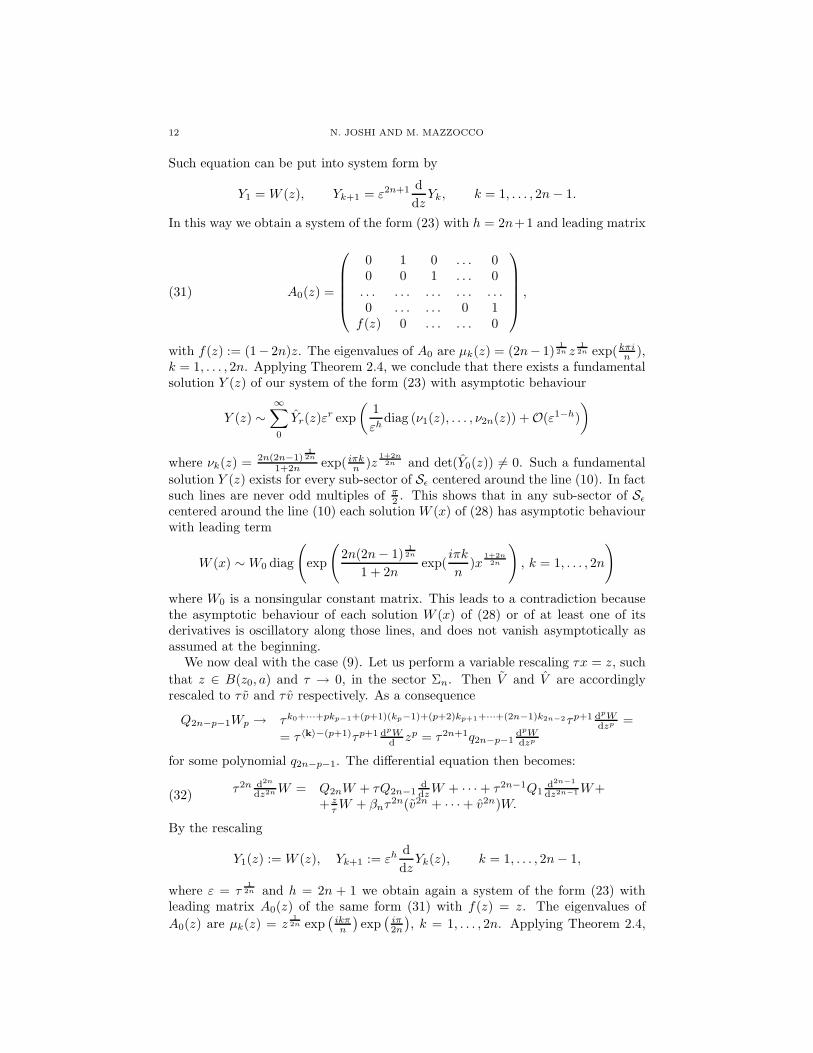
Such equation can be put into system form by

Y1 = W (z), Yk+1 = ε2n+1 d

dzYk, k = 1, . . . , 2n − 1.

In this way we obtain a system of the form (23) with h = 2n+1 and leading matrix

(31) A0(z) =

0 1 0 . . . 00 0 1 . . . 0

. . . . . . . . . . . . . . .0 . . . . . . 0 1

f(z) 0 . . . . . . 0

,

with f(z) := (1− 2n)z. The eigenvalues of A0 are µk(z) = (2n− 1)12n z

12n exp(kπi

n ),k = 1, . . . , 2n. Applying Theorem 2.4, we conclude that there exists a fundamentalsolution Y (z) of our system of the form (23) with asymptotic behaviour

Y (z) ∼∞∑

0

Yr(z)εr exp

(

1

εhdiag (ν1(z), . . . , ν2n(z)) + O(ε1−h)

)

where νk(z) = 2n(2n−1)12n

1+2n exp( iπkn )z

1+2n2n and det(Y0(z)) 6= 0. Such a fundamental

solution Y (z) exists for every sub-sector of Sǫ centered around the line (10). In factsuch lines are never odd multiples of π

2 . This shows that in any sub-sector of Sǫ

centered around the line (10) each solution W (x) of (28) has asymptotic behaviourwith leading term

W (x) ∼ W0 diag

(

exp

(

2n(2n− 1)12n

1 + 2nexp(

iπk

n)x

1+2n2n

)

, k = 1, . . . , 2n

)

where W0 is a nonsingular constant matrix. This leads to a contradiction becausethe asymptotic behaviour of each solution W (x) of (28) or of at least one of itsderivatives is oscillatory along those lines, and does not vanish asymptotically asassumed at the beginning.

We now deal with the case (9). Let us perform a variable rescaling τx = z, such

that z ∈ B(z0, a) and τ → 0, in the sector Σn. Then V and V are accordinglyrescaled to τ v and τ v respectively. As a consequence

Q2n−p−1Wp → τk0+···+pkp−1+(p+1)(kp−1)+(p+2)kp+1+···+(2n−1)k2n−2τp+1 dpWdzp =

= τ 〈k〉−(p+1)τp+1 dpWd zp = τ2n+1q2n−p−1

dpWdzp

for some polynomial q2n−p−1. The differential equation then becomes:

(32)τ2n d2n

dz2n W = Q2nW + τQ2n−1ddz W + · · · + τ2n−1Q1

d2n−1

dz2n−1 W++ z

τ W + βnτ2n(v2n + · · · + v2n)W.

By the rescaling

Y1(z) := W (z), Yk+1 := εh d

dzYk(z), k = 1, . . . , 2n − 1,

where ε = τ12n and h = 2n + 1 we obtain again a system of the form (23) with

leading matrix A0(z) of the same form (31) with f(z) = z. The eigenvalues of

A0(z) are µk(z) = z12n exp

(

ikπn

)

exp(

iπ2n

)

, k = 1, . . . , 2n. Applying Theorem 2.4,


we conclude that there exists a fundamental solution Y (z) of our system of theform (23) with asymptotic behaviour

Y (z) ∼

∞∑

0

Yr(z)εr exp

(

1

εhdiag (ν1(z), . . . , ν2n(z))

)

where νk(z) = 2n1+2n exp

(

iπ2n

)

exp( iπkn )z

1+2n2n and det(Y0(z)) 6= 0. Such solution

Y (z) exists for every sub-sector of Sǫ centered around the line (11). In fact suchlines are never odd multiples of π

2 . This shows that in any sub-sector of Sǫ centeredaround the line (11) each solution W (x) of (28) has asymptotic behaviour withleading term

W (x) ∼ W0 diag

(

exp

(

2n

1 + 2nexp

(

iπ

2n

)

exp

(

iπk

n

)

x1+2n2n

)

k = 1, . . . , 2n

)

where W0 is a non-singular constant matrix. This leads to a contradiction becausethe asymptotic behaviour of each solution W (x) of (28) or of at least one of itsderivatives is oscillatory along those lines, and not vanishing asymptotically asassumed at the beginning.

References

[1] M. J. Ablowitz and H. Segur. Exact linearization of a Painleve transcendent. Phys. Rev. Lett.,38:1103–1106, 1977.

[2] H. Airault. Rational solutions of Painleve equations. Studies in Applied Mathematics, 61:31–53, 1979.

[3] P. Boutroux. Recherches sur les transcendantes de M. Painleve et l’etude asymptotique des

equations differentielles du second ordre. Ann. Ecole Norm., 30:265–375, 1913.[4] P. Boutroux. Recherches sur les transcendantes de M. Painleve et l’etude asymptotique des

equations differentielles du second ordre. Ann. Ecole Norm., 31:99–159, 1914.[5] P. A. Clarkson and N. Joshi and M. Mazzocco. The Lax pair for the mKdV hierarchy. preprint,

2002.[6] P. A. Clarkson and N. Joshi and A. Pickering. Backlund transformations for the second

Painleve hierarchy: a modified truncation approach. Inverse Problems, 15:175–187, 1999.[7] H. Flaschka and A. C. Newell. Monodromy and Spectrum Preserving Deformations I. Comm.

Math. Phys., 76:65–116, 1980.[8] R. Haberman. The modulated phase shift for weakly dissipated nonlinear oscillatory waves of

the Korteweg-de Vries type. Stud. Appl. Math., 78, no. 1, 73–90 1988.[9] R. Haberman. Nonlinear transition layers—the second Painleve transcendent. Stud. Appl.

Math., 57, no. 3, 247–270, 1977.[10] N. Joshi and M. D. Kruskal. The Painleve connection problem: an asymptotic approach I.

Stud. Appl. Math., 86:315–376, 1992.[11] P. D. Lax. Almost periodic solutions of the KdV equation. SIAM review, 18, no.3:351–375,

1976.[12] R. C. Littlewood. Hyperelliptic asymptotics of Painleve–type equations. Nonlinearity, 12,

1629–1641, 1999.[13] P. Painleve. Sur les Equations Differentielles du Second Ordre et d’Ordre Superieur, dont

l’Interable Generale est Uniforme. Acta Math., 25:1–86, 1902.[14] Y. Sibuya. Linear Differential Equations in the Complex Domain: Problems of Analytic

Continuation. AMS TMM, 82, 1990.[15] H. Umemura. Second Proof of the Irreducibility of the First Differential Equation of Painleve.

Nagoya Math. J., 117:125–171, 1990.

[16] H. Umemura and H. Watanabe. Solutions of the Second and Fourth Painleve Equations. I.Nagoya Math. J., 148:151–198, 1997.

[17] W. Wasow. Asymptotic Expansions for Ordinary differential Equations. Pure and Applied

Mathematics, John Wiley and Sons, Inc., XIV, 1965.


School of Mathematics and Statistics F07, University of Sydney, NSW2006 Sydney,

Australia

E-mail address: [email protected]

Mathematical Institute, University of Oxford, 24-29 St Giles, Oxford OX1 3LB, UK

and DPMMS, Wilberforce Road, Cambridge CB3 0WB, UK.

E-mail address: [email protected]

Existence and uniqueness of tri-tronqu e solutions of the second Painlev hierarchy

Documents

Transcript of Existence and uniqueness of tri-tronqu e solutions of the second Painlev hierarchy