CORE DISCUSSION PAPER

2003/83

Optimal Growth Models and theLagrange Multiplier∗

Cuong Le Van†, H. Cagri Saglam‡

November 2003

Abstract

We provide sufficient conditions on the objective functional and theconstraint functions under which the Lagrangean can be represented by a`1 sequence of multipliers in infinite horizon discrete time optimal growthmodels.

Keywords: Optimal Growth, Lagrange Multipliers.

JEL Classification: C61, O41.

∗The authors thank the referee for criticisms, remarks and suggestions. They also thankYiannis Vailakis for helpful comments. This text presents research results of the BelgianProgram on Interuniversity Poles of Attraction initiated by the Belgian State, Prime Minister’sOffice, Science Policy Programming. The scientific responsibility is assumed by the authors.

†CNRS, CERMSEM, Université de Paris 1, CORE. E-mail: cuong.le-van@univ-paris1.fr‡IRES, Université catholique de Louvain. E-mail: saglam@ires.ucl.ac.be

1 IntroductionThe classical optimal growth models have played a central role in the theoryof economic dynamics. The model is described by the presence of a plannermaximizing the sum of discounted utilities of consumption subject to a convexone-sector production set. This simple and elegant model proves to be useful inexplaining many aspects of capital accumulation.1

The study of this type of optimal capital accumulation problems can beconsiderably enhanced by means of Lagrange multipliers techniques.2 Lagrangemultipliers have been widely used in solving finite dimensional constrainedoptimization problems as they also facilitate the analysis on the properties ofthe solution [see Rockafellar (1976)]. However, in infinite horizon optimal growthmodels, these multipliers will typically belong to an infinite dimensional decisionspace. Therefore, the questions whether the Lagrange multipliers exist andwhether they can be represented by a summable sequence arise.3

In this paper we extend the Lagrangean to infinite dimensional spaces andprovide sufficient conditions for Lagrangean to be represented by a summablesequence of multipliers in infinite discrete time horizon optimal growth models.We take the approach of placing restrictions directly on the asymptotic behaviorsof the objective functional and the constraint functions. In this sense, our workis closely related to Dechert (1982).

Considering the set of problems in the form of: inf {F (x) | φ (x) ≤ 0} , whereF : `∞ → R and φ : `∞ → `∞ are convex functions and x ∈ `∞, Dechert (1982)extends the Lagrangean to infinite dimensional spaces. However, a limitationto the direct use of his results in infinite horizon optimal growth models stemsfrom the fact that he assumes that the objective functional and the constraintfunctions are real valued on `∞. That avoids the analysis of the cases where theusual Inada type conditions are assumed for the utility (in this case there is noextension of utility value to R) and the production functions.

The paper is organized as follows. In section 2, we first present the problemin general form and give the extension of the Kuhn-Tucker theorem where themultipliers are represented in (`∞)p , the dual space of `∞. Second, we presentthe sufficient conditions for having an `1 representation of the multipliers andstate our main result. Finally, section 3 is devoted to the applications to aone-sector optimal growth model and an incentive-constrained optimal growthmodel.

1See Aliprantis, Border and Burkinshaw (1990, 1997) for some recent studies and Stokeyet al. (1989) for more details.

2Dynamic programming is another technique used in analyzing such models; see for in-stance Alvarez and Stokey (1998), Le Van and Morhaim (2002). See also Weitzman (1973) forthe close connection between duality theory for infinite horizon convex models and dynamicprogramming.

3The existence of separating vectors and whether they can be represented by a sequence ofreal numbers in infinite dimensional spaces have been widely studied; see for instance Bewley(1972), Majumdar (1972), Colonius (1983), Rustichini (1998) and McKenzie (1986).

1

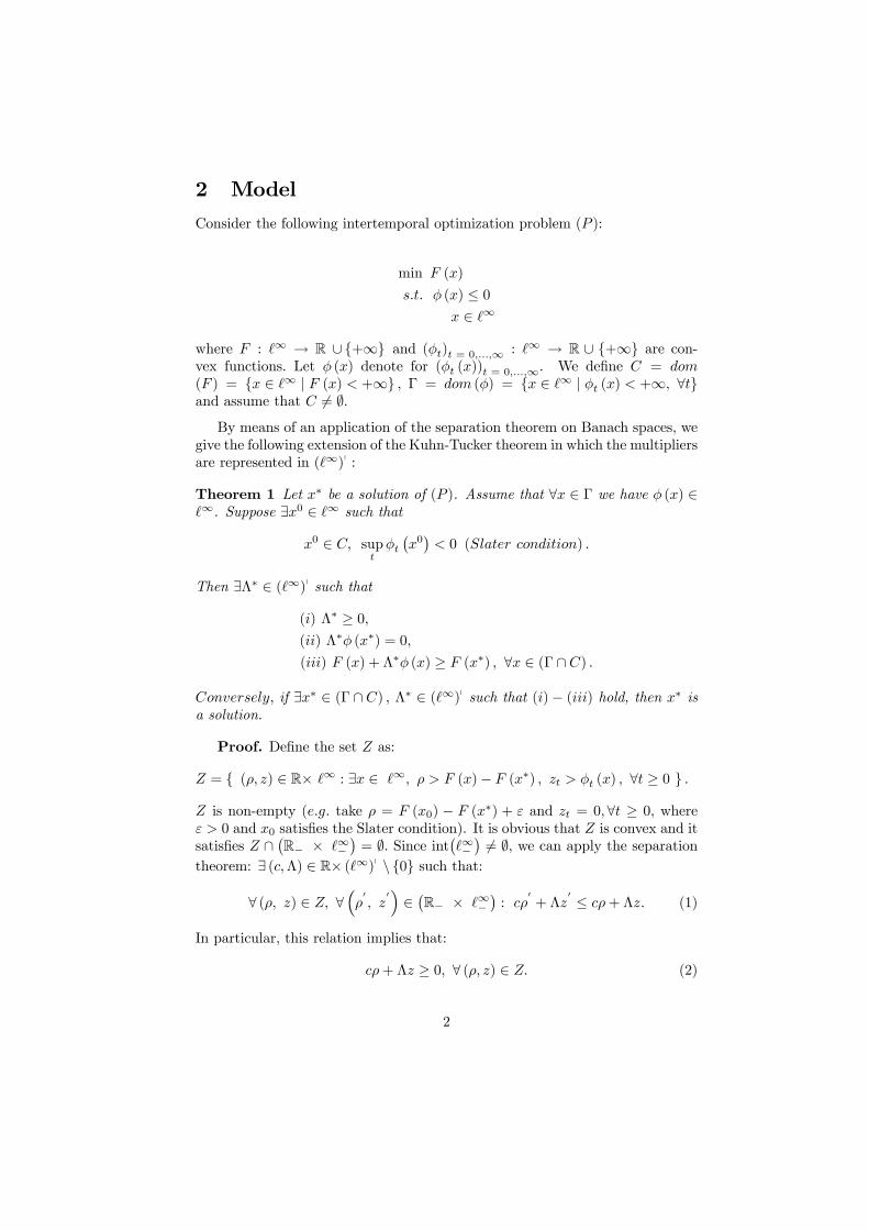
2 ModelConsider the following intertemporal optimization problem (P ):

min F (x)

s.t. φ (x) ≤ 0x ∈ `∞

where F : `∞ → R ∪ {+∞} and (φt)t = 0,...,∞ : `∞ → R ∪ {+∞} are con-vex functions. Let φ (x) denote for (φt (x))t = 0,...,∞. We define C = dom(F ) = {x ∈ `∞ | F (x) < +∞} , Γ = dom (φ) = {x ∈ `∞ | φt (x) < +∞, ∀t}and assume that C 6= ∅.By means of an application of the separation theorem on Banach spaces, we

give the following extension of the Kuhn-Tucker theorem in which the multipliersare represented in (`∞)p :

Theorem 1 Let x∗ be a solution of (P ). Assume that ∀x ∈ Γ we have φ (x) ∈`∞. Suppose ∃x0 ∈ `∞ such that

x0 ∈ C, suptφt¡x0¢< 0 (Slater condition) .

Then ∃Λ∗ ∈ (`∞)p such that

(i) Λ∗ ≥ 0,(ii) Λ∗φ (x∗) = 0,(iii) F (x) + Λ∗φ (x) ≥ F (x∗) , ∀x ∈ (Γ ∩C) .

Conversely, if ∃x∗ ∈ (Γ ∩C) , Λ∗ ∈ (`∞)p such that (i)− (iii) hold, then x∗ isa solution.

Proof. Define the set Z as:

Z = { (ρ, z) ∈ R× `∞ : ∃x ∈ `∞, ρ > F (x)− F (x∗) , zt > φt (x) , ∀t ≥ 0 } .

Z is non-empty (e.g. take ρ = F (x0) − F (x∗) + ε and zt = 0,∀t ≥ 0, whereε > 0 and x0 satisfies the Slater condition). It is obvious that Z is convex and itsatisfies Z ∩ ¡R− × `∞−

¢= ∅. Since int¡`∞− ¢ 6= ∅, we can apply the separation

theorem: ∃ (c,Λ) ∈ R× (`∞)p \ {0} such that:

∀ (ρ, z) ∈ Z, ∀³ρ0, z

0´ ∈ ¡R− × `∞−¢: cρ

0+ Λz

0 ≤ cρ+ Λz. (1)

In particular, this relation implies that:

cρ+ Λz ≥ 0, ∀ (ρ, z) ∈ Z. (2)

2

Note that (ρ, z) ∈ Z if ρ > 0 and zt > 0, ∀t (take x = x∗ in the definition of Z).We first want to prove that c ≥ 0. On the contrary, if c < 0 then keeping z

fixed and letting ρ→ +∞ in (2), we obtain a contradiction. Hence c ≥ 0.Now we claim that Λ ∈ (`∞)p+ , i.e. Λz ≥ 0, ∀z ∈ `∞+ . For that, take z ∈ `∞+ .

Let θ = (1, 1, 1, ...1, ...) and ρ = 1. Then, (ρ, θ + µz) ∈ Z for any µ > 0.From relation (2), we notice that cρ + Λ (θ + µz) ≥ 0, ∀µ > 0 or equivalentlyµ−1 (cρ+ Λθ) + Λz ≥ 0, ∀µ > 0. Letting µ → +∞, we obtain that Λz ≥ 0,∀z ∈ `∞+ . Hence, Λ ∈ (`∞)p+ .We now prove that c > 0. Assume on the contrary that c = 0. In this case,

we know that Λ 6= 0. Note that the closure of Z is:_Z = { (z0, z) ∈ R× `∞ : ∃x ∈ `∞, z0 ≥ F (x)− F (x∗) , zt ≥ φt (x) ,∀t } .Observe that we still have,

cρ+ Λz ≥ 0, ∀ (ρ, z) ∈_Z. (3)

As¡F¡x0¢− F (x∗) , φ ¡x0¢¢ ∈ _

Z, from (3), we obtain a contradiction:

0 > Λφ¡x0¢ ≥ 0,

due to the fact that suptφt¡x0¢< 0.

Let Λ∗ = c−1Λ in order to obtain the claim (i) of the theorem. Now, we provethe claim (ii) of the theorem. Since Λ∗ ≥ 0, (0, φ (x∗)) ∈

_Z and φ (x∗) ∈ `∞− ,

we have on the one hand Λ∗φ (x∗) ≤ 0 and Λ∗φ (x∗) ≥ 0 on the other. Hence,Λ∗φ (x∗) = 0.

Finally, take z0 = F (x) − F (x∗) and z = φ (x) , ∀x ∈ (Γ ∩ C) . Then, frominequality (3), we obtain that:

F (x)− F (x∗) + Λ∗φ (x) ≥ 0⇒F (x) + Λ∗φ (x) ≥ F (x∗) + Λ∗φ (x∗) , ∀x ∈ (Γ ∩ C) .

As for the converse, let x ∈ `∞ satisfy φ (x) ≤ 0. Then, x ∈ Γ. If x /∈ C thenF (x) = +∞ and of course we have F (x) ≥ F (x∗) . Now assume that x ∈ C.Relations (i), (ii) and (iii) imply that

F (x) ≥ F (x) + Λ∗φ (x) ≥ F (x∗) + Λ∗φ (x∗) = F (x∗) .Thus, we have proved that x∗ is an optimal solution.

Corollary 1 Let the assumptions of Theorem 1 be satisfied. If x∗ (solution tothe optimization problem P ) satisfies that x∗ ∈ int (Γ ∩ C) , then we have

∀x ∈ `∞, F (x) + Λ∗φ (x) ≥ F (x∗) + Λ∗φ (x∗)where Λ∗ ∈ (`∞)p+ and Λ∗φ (x∗) = 0.

3

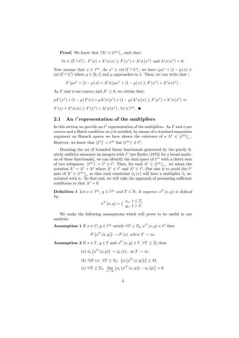
Proof. We know that ∃Λ∗ ∈ (`∞)p+ such that:∀x ∈ (Γ ∩ C) , F (x) + Λ∗φ (x) ≥ F (x∗) + Λ∗φ (x∗) and Λ∗φ (x∗) = 0.

Now assume that x ∈ `∞. As x∗ ∈ int (Γ ∩ C) , we have (µx∗ + (1− µ)x) ∈int (Γ ∩ C) where µ ∈ [0, 1] and µ approaches to 1. Then, we can write that :

F (µx∗ + (1− µ)x) + Λ∗φ (µx∗ + (1− µ)x) ≥ F (x∗) + Λ∗φ (x∗) .As F and φ are convex and Λ∗ ≥ 0, we obtain that:µF (x∗)+(1− µ)F (x)+µΛ∗φ (x∗)+ (1− µ)Λ∗φ (x) ≥ F (x∗)+Λ∗φ (x∗)⇒F (x) + Λ∗φ (x) ≥ F (x∗) + Λ∗φ (x∗) , ∀x ∈ `∞.

2.1 An `1representation of the multipliers

In this section we provide an `1 representation of the multipliers. As F and φ areconvex and a Slater condition on φ is satisfied, by means of a standard separationargument on Banach spaces we have shown the existence of a Λ∗ ∈ (`∞)p+ .However, we know that

¡`1¢p= `∞ but (`∞)p 6= `1.

Denoting the set of bounded linear functionals generated by the purely fi-nitely additive measures on integers with `s [see Rudin (1973) for a broad analy-sis of those functionals], we can identify the dual space of `∞ with a direct sumof two subspaces: (`∞)p = `1 ⊕ `s. Then, for each Λ∗ ∈ (`∞)p+ , we adopt thenotation Λ∗ = Λ1 + Λs where Λ1 ∈ `1 and Λs ∈ `s. Our aim is to avoid the `s

part of Λ∗ ∈ (`∞)p+ so that each constraint φt (x) will have a multiplier λt as-sociated with it. To that end, we will take the approach of presenting sufficientconditions so that Λs = 0.

Definition 1 Let x ∈ `∞, y ∈ `∞ and T ∈ N. A sequence xT (x, y) is definedby:

xT (x, y) = { xt, t ≤ T,yt, t > T.

We make the following assumptions which will prove to be useful in ouranalysis:

Assumption 1 If x ∈ C, y ∈ `∞ satisfy ∀T ≥ T0, xT (x, y) ∈ C thenF¡xT (x, y)

¢→ F (x) when T →∞.Assumption 2 If x ∈ Γ, y ∈ Γ and xT (x, y) ∈ Γ, ∀T ≥ T0 then

(a) φt¡xT (x, y)

¢→ φt (x) , as T →∞,

(b) ∃M s.t. ∀T ≥ T0,°°φ ¡xT (x, y)¢°° ≤M,

(c) ∀N ≥ T0, limt→∞

£φt¡xN (x, y)

¢− φt (y)¤= 0.

4

We also adopt the following conventions [see Rockafellar (1976)] in our analysis:

0 (+∞) = (+∞) 0 = 0,α (+∞) = (+∞) α = +∞ if α > 0.

We have the following remark on the assumptions we have made:

Remark 1 Assumption 1 is satisfied if F is continuous in C =dom(F ) for theproduct topology. Assumption 2-(a) is the asymptotically non-anticipatory as-sumption (ANA) and Assumption 2-(c) is true if the asymptotically insensitivity(AI) assumption holds [see Dechert (1982)] for φ in Γ = dom (φ) . Obviously,Assumption 2-(b) is satisfied when Γ = dom (φ) = `∞ and φ is continuous.

More precisely, the restrictions on φ that we use lead to the following twolemmas :

Lemma 1 Under Assumption 2-(c), we have:

Λsφ¡xN (x, y)

¢= Λsφ (y) , for any N ≥ T0.

Proof. Follows directly from the property of `s. Indeed, for any Λs ∈ `s andx ∈ `∞ with lim

t→∞x (t) = 0, Λsx = 0.GivenN, as lim

t→∞£φt¡xN (x, y)

¢− φt (y)¤=

0, we haveΛs£φ¡xN (x, y)

¢− φ (y)¤= 0,

completing the proof.

Lemma 2 Let Assumptions (2-a) and (2-b) be satisfied. Then, ∀Λ1 ∈ `1,limT→∞

Λ1φ¡xT (x, y)

¢= Λ1φ (x) .

Proof. We have for T ≥ T0,¯̄Λ1φ

¡xT (x, y)

¢− Λ1φ (x)¯̄ ≤NXt=0

|λt|¯̄φt¡xT (x, y)

¢− φt (x)¯̄+°°φ ¡xT (x, y)¢− φ (x)

°° ∞Xt=N+1

|λt| .

By Assumption (2-b), we know that ∃M such that:

∀T,°°φ ¡xT (x, y)¢− φ (x)°° ≤M 0 =M + kφ (x)k .

Now, ∀ε > 0, ∃N0 such that:∞X

t=N0+1

|λt| <³2M

0´−1ε,

and ∃T t ≥ T0, ∀T > T t,|λt|

¯̄φt¡xT (x, y)

¢− φt (x)¯̄< (2N0)

−1 ε.

5

Hence, ∀T > max1≤t≤N0

{T t} ,

¯̄Λ1φ

¡xT (x, y)

¢− Λ1φ (x)¯̄ < N0 (2N0)−1 ε+M 0 ³2M

0´−1ε = ε,

completes the proof.

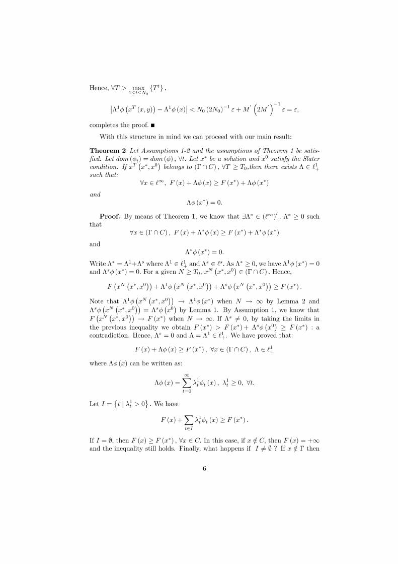
With this structure in mind we can proceed with our main result:

Theorem 2 Let Assumptions 1-2 and the assumptions of Theorem 1 be satis-fied. Let dom (φt) = dom (φ) , ∀t. Let x∗ be a solution and x0 satisfy the Slatercondition. If xT

¡x∗, x0

¢belongs to (Γ ∩ C) , ∀T ≥ T0,then there exists Λ ∈ `1+

such that:∀x ∈ `∞, F (x) + Λφ (x) ≥ F (x∗) + Λφ (x∗)

andΛφ (x∗) = 0.

Proof. By means of Theorem 1, we know that ∃Λ∗ ∈ (`∞)0 , Λ∗ ≥ 0 suchthat

∀x ∈ (Γ ∩C) , F (x) + Λ∗φ (x) ≥ F (x∗) + Λ∗φ (x∗)and

Λ∗φ (x∗) = 0.

Write Λ∗ = Λ1+Λs where Λ1 ∈ `1+ and Λs ∈ `s.As Λ∗ ≥ 0, we have Λ1φ (x∗) = 0and Λsφ (x∗) = 0. For a given N ≥ T0, xN

¡x∗, x0

¢ ∈ (Γ ∩ C) . Hence,F¡xN¡x∗, x0

¢¢+ Λ1φ

¡xN¡x∗, x0

¢¢+ Λsφ

¡xN¡x∗, x0

¢¢ ≥ F (x∗) .Note that Λ1φ

¡xN¡x∗, x0

¢¢ → Λ1φ (x∗) when N → ∞ by Lemma 2 andΛsφ

¡xN¡x∗, x0

¢¢= Λsφ

¡x0¢by Lemma 1. By Assumption 1, we know that

F¡xN¡x∗, x0

¢¢ → F (x∗) when N → ∞. If Λs 6= 0, by taking the limits inthe previous inequality we obtain F (x∗) > F (x∗)+ Λsφ

¡x0¢ ≥ F (x∗) : a

contradiction. Hence, Λs = 0 and Λ = Λ1 ∈ `1+. We have proved that:F (x) + Λφ (x) ≥ F (x∗) , ∀x ∈ (Γ ∩ C) , Λ ∈ `1+

where Λφ (x) can be written as:

Λφ (x) =∞Xt=0

λ1tφt (x) , λ1t ≥ 0, ∀t.

Let I =©t | λ1t > 0

ª. We have

F (x) +Xt∈I

λ1tφt (x) ≥ F (x∗) .

If I = ∅, then F (x) ≥ F (x∗) , ∀x ∈ C. In this case, if x /∈ C, then F (x) = +∞and the inequality still holds. Finally, what happens if I 6= ∅ ? If x /∈ Γ then

6

Pt∈I

λ1tφt (x) = +∞. Since F (x) ∈ R ∪ {+∞} , we have F (x)+Pt∈I

λ1tφt (x) = +∞so that the inequality F (x)+Λφ (x) ≥ F (x∗) holds. On the other hand, if x ∈ Γand x /∈ C we have also F (x)+P

t∈Iλ1tφt (x) = +∞ and F (x)+Λφ (x) ≥ F (x∗) .

Thus, ∀x ∈ `∞, F (x) + Λφ (x) ≥ F (x∗) .

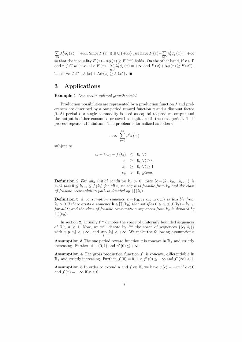
3 ApplicationsExample 1 One-sector optimal growth model

Production possibilities are represented by a production function f and pref-erences are described by a one period reward function u and a discount factorβ. At period t, a single commodity is used as capital to produce output andthe output is either consumed or saved as capital until the next period. Thisprocess repeats ad infinitum. The problem is formalized as follows:

max∞Xt=0

βtu (ct)

subject to

ct + kt+1 − f (kt) ≤ 0, ∀tct ≥ 0, ∀t ≥ 0kt ≥ 0, ∀t ≥ 1k0 > 0, given.

Definition 2 For any initial condition k0 > 0, when k =(k1, k2, ...kt, ...) issuch that 0 ≤ kt+1 ≤ f (kt) for all t, we say it is feasible from k0 and the classof feasible accumulation path is denoted by

Q(k0) .

Definition 3 A consumption sequence c =(c0, c1, c2, ...ct, ...) is feasible fromk0 > 0 if there exists a sequence k ∈

Q(k0) that satisfies 0 ≤ ct ≤ f (kt)− kt+1,

for all t; and the class of feasible consumption sequences from k0 is denoted byP(k0) .

In section 2, actually `∞ denotes the space of uniformly bounded sequencesof Rn, n ≥ 1. Now, we will denote by `∞ the space of sequences {(ct, kt)}with sup

t|ct| < +∞ and sup

t|kt| < +∞. We make the following assumptions:

Assumption 3 The one period reward function u is concave in R+ and strictlyincreasing. Further, β ∈ (0, 1) and u0 (0) ≤ +∞.Assumption 4 The gross production function f is concave, differentiable inR+ and strictly increasing. Further, f (0) = 0, 1 < f 0 (0) ≤ +∞ and f 0 (∞) < 1.Assumption 5 In order to extend u and f on R, we have u (c) = −∞ if c < 0and f (x) = −∞ if x < 0.

7

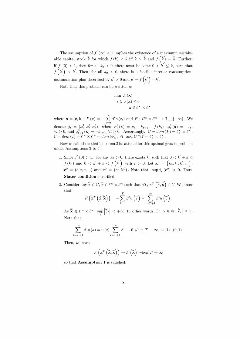
The assumption of f0(∞) < 1 implies the existence of a maximum sustain-

able capital stock_

k for which f (k) < k iff k >_

k and f³_k´=

_

k. Further,

if f0(0) > 1, then for all k0 > 0, there must be some 0 < k

0 ≤ k0 such thatf³k0´> k

0. Then, for all k0 > 0, there is a feasible interior consumption-

accumulation plan described by k0> 0 and c

0= f

³k0´− k0 .

Note that this problem can be written as

min F (x)

s.t. φ (x) ≤ 0x ∈ `∞ × `∞

where x =(c,k) , F (x) = −∞Pt=0

βtu (ct) and F : `∞ × `∞ → R ∪ {+∞} . Wedenote φt = (φ1t ,φ

2t ,φ

3t ) where φ1t (x) = ct + kt+1 − f (kt) , φ2t (x) = −ct,

∀t ≥ 0, and φ3t+1 (x) = −kt+1, ∀t ≥ 0. Accordingly, C = dom (F ) = `∞+ × `∞,Γ = dom (φ) = `∞ × `∞+ = dom (φt) , ∀t and C ∩ Γ = `∞+ × `∞+ .Now we will show that Theorem 2 is satisfied for this optimal growth problem

under Assumptions 3 to 5:

1. Since f0(0) > 1. for any k0 > 0, there exists k

0such that 0 < k

0+ ε <

f (k0) and 0 < k0+ ε < f

³k0´with ε > 0. Let k0 =

³k0, k

0, k

0, ...´,

c0 = (ε, ε, ε, ...) and x0 =¡c0,k0

¢. Note that sup

tφt¡c0¢< 0. Thus,

Slater condition is verified.

2. Consider any∼x ∈ C, ≈x ∈ `∞× `∞ such that ∀T, xT

³∼x,≈x´∈ C.We know

that:

F³xT³∼x,≈x´´= −

TXt=0

βtu³∼c´−

∞Xt=T+1

βtu³≈c´.

As≈x ∈ `∞ × `∞, sup

t

¯̄̄≈c t

¯̄̄< +∞. In other words, ∃a > 0,∀t,

¯̄̄≈c t

¯̄̄≤ a.

Note that,

∞Xt=T+1

βtu (a) = u (a)∞X

t=T+1

βt → 0 when T →∞, as β ∈ (0, 1) .

Then, we have

F³xT³∼x,≈x´´→ F

³∼x´when T →∞

so that Assumption 1 is satisfied.

8

3. Let x = (c,k) , kt ≥ 0,∀t and y = (c0,k0) , k0t ≥ 0,∀t. We have:

φ1t¡xT (x,y)

¢= { ct + kt+1 − f (kt) < +∞, if t < T

c0t + k0t+1 − f (k0t) < +∞, if t > T

andφ1T¡xT (x,y)

¢= cT + k

pT+1 − f (kT ) < +∞.

Then, xT (x,y) ∈ Γ, ∀T. It is evident that if T > t+ 1, we have:

φ1t¡¡xT (x,y)

¢¢= φ1t (x).

It is clear that the same is also true for φ2t¡xT (x,y)

¢and φ3t

¡xT (x,y)

¢,

as well. Thus, Assumption 2-(a) is satisfied.

4. For any x ∈ Γ, y ∈ Γ, let

M1 = kφ (x)k∞ = supt≥0

|φt (x)|

andM2 = kφ (y)k∞ = sup

t≥0|φt (y)| .

Knowing that

xT (x,y) = { xt, t ≤ Tyt, t > T

and simply setting M = max {M1,M2} lead us to conclude that ∃M such

that, ∀T,°°°°φµxT µx∼, y∼

¶¶°°°° ≤ M . This proves that Assumption 2-(b)is satisfied.

5. We know that

∀N, φt¡xT (x,y)

¢= { φt (x) , t ≤ N

φt (y) , t > N

Let∧t = N + 1. Then we have φt

¡xT (x,y)

¢= φt (y) , when t >

∧t > N.

Thus, Assumption 2-(c) is satisfied.

6. It is obvious that xT¡x∗,x0

¢belongs to `∞+ × `∞+ , ∀T.

Summimg up, we have shown that the assumptions of Theorem 2 are fulfilledfor our optimal growth problem. Hence there exists Λ ∈ `1+ such that ∀x ∈ `∞,if x∗ is optimal, then

F (x) + Λφ (x) ≥ F (x∗) + Λφ (x∗) and Λφ (x∗) = 0.

These establish the following proposition.

9

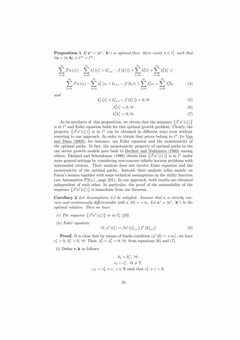
Proposition 1 If x∗ = (c∗, k∗) is optimal then there exists λ ∈ `1+ such that∀x = (c,k) ∈ `∞ × `∞,∞Xt=0

βtu (c∗t )−∞Xt=0

λ1t¡c∗t + k

∗t+1 − f (k∗t )

¢+∞Xt=0

λ2t c∗t +

∞Xt=0

λ3tk∗t ≥

∞Xt=0

βtu (ct)−∞Xt=0

λ1t (ct + kt+1 − f (kt)) +∞Xt=0

λ2t ct +∞Xt=0

λ3tkt (4)

andλ1t¡c∗t + k

∗t+1 − f (k∗t )

¢= 0,∀t (5)

λ2t c∗t = 0,∀t (6)

λ3tk∗t = 0,∀t. (7)

As by-products of this proposition, we obtain that the sequence©βtu0 (c∗t )

ªis in `1 and Euler equation holds for this optimal growth problem. Clearly, theproperty

©βtu0 (c∗t )

ªis in `1 can be obtained in different ways even without

resorting to our approach. In order to obtain that prices belong to `1, Le Vanand Dana (2003), for instance, use Euler equation and the monotonicity ofthe optimal paths. In fact, the monotonicity property of optimal paths in theone sector growth models goes back to Dechert and Nishimura (1983) amongothers. Ekeland and Scheinkman (1986) obtain that

©βtu0 (c∗t )

ªis in `1 under

more general settings by considering non-concave infinite horizon problems withunbounded returns. Their analysis does not involve Euler equation and themonotonicity of the optimal paths. Instead, their analysis relies mainly onFatou’s lemma together with some technical assumptions on the utility function(see Assumption P2(ct) , page 221). In our approach, both results are obtainedindependent of each other. In particular, the proof of the summability of thesequence

©βtu0 (c∗t )

ªis immediate from our theorem.

Corollary 2 Let Assumptions 3-5 be satisfied. Assume that u is strictly con-cave and continuously differentiable with u

0(0) = +∞. Let x∗ = (c∗, k∗) be the

optimal solution. Then we have:

(i) The sequence©βtu0 (c∗t )

ªis in `1+\{0}.

(ii) Euler equation:∀t, u0 (c∗t ) = βu0

¡c∗t+1

¢f 0¡k∗t+1

¢(8)

Proof. It is clear that by means of Inada condition (u0 (0) = +∞) , we havec∗t > 0, k∗t > 0, ∀t. Thus, λ2t = λ3t = 0, ∀t, from equations (6) and (7).

(i) Define c,k as follows:

kt = k∗t , ∀t,

ct = c∗t , ∀t 6= T,

cT = c∗T + ε, ε ∈ R such that c∗T + ε > 0.

10

Inequality (4) implies that:

βTu (c∗T )− λ1T c∗T ≥ βTu (c∗T + ε)− λ1T (c∗T + ε) ,

for any ε in a neighborhood of zero. This implies:

βTu0 (c∗T )− λ1T = 0.

Since, from Proposition 1, λ ∈ `1+, then³βTu0 (c∗T )

´∈ `1+.

(ii) Define

ct = c∗t , ∀t

kt = k∗T , ∀t 6= T + 1

kT+1 = k∗T+1 + ε, ε ∈ R such that k∗T+1 + ε > 0.

By (4), we have:

−λ1T k∗T+1 + λ1T+1 f¡k∗T+1

¢ ≥ −λ1T ¡k∗T+1 + ε

¢+ λ1T+1 f

¡k∗T+1 + ε

¢,

for any ε in a neighborhood of zero. Therefore,

−λ1T + λ1T+1f0 ¡k∗T+1

¢= 0.

From (i), we know that λ1T = βTu0 (c∗T ) . Hence, Euler equation follows.

Remark 2 In order to have an `1 representation of Lagrangean, Dechert (1982)introduces the hypothesis that:

∂F (x∗) ⊂ `1,together with two constraint conditions: φ is asymptotically insensitive (AI) andnon-anticipatory (ANA). Contrary to Dechert (1982), the hypothesis ∂F (x∗) ⊂`1 is not necessarily verified. Indeed, suppose that f

0(0) < 1

β . Let u be differen-tiable in R+ with u0 (0) = +∞. If ∂F (x∗) ⊂ `1, then we will have:

∂F (x∗) =©¡u0 (c∗0) , βu

0 (c∗1) , ... , βtu0 (c∗t ) , ...

¢ª.

Hence, F is differentiable at x∗ and thus, continuous at x∗ (for the topology`∞). Hence, ∀ε > 0, ∃η,

supt|c∗t − ct| ≤ η ⇒

¯̄̄̄¯∞Xt=0

βtu (c∗t )−∞Xt=0

βtu (ct)

¯̄̄̄¯ ≤ ε.

We know that c∗t → 0. Then, ∃T, ∀t ≥ T, 0 ≤ c∗t < η. So define ct = c∗t ,t 6= T and cT = c∗T − η < 0. (c0, ...ct, ...) verifies sup

t|c∗t − ct| = η and u (ct) =

−∞. Thus,¯̄̄βTu (c∗T )− βTu (cT )

¯̄̄= +∞ and

¯̄̄̄ ∞Pt=0

βtu (c∗t )−∞Pt=0

βtu (ct)

¯̄̄̄≤

ε, does not hold.

11

Remark 3 The assumption that f 0(0) > 1 is crucial to have multipliers in `1.Indeed, assume, on the contrary, that f 0(0) ≤ 1. Assume that Inada conditionholds. We then have the Euler equation:

−λ1T + λ1T+1f0 ¡k∗T+1

¢= 0.

Since f 0 is decreasing, we have f0 ¡k∗T+1

¢ ≤ f 0(0) ≤ 1. Hence λ1T+1 ≥ λ1T , ∀T .In other words, λ1T ≥ λ10 = u

0(c∗0) > 0,∀T. That proves that the multipliers λ1

are not in `1.

Example 2 The Recursive Utility and Optimal Growth

In the previous example, one can use the support prices approach accordingto Weitzman (1973) and McKenzie (1986) tradition. But this approach is spe-cific to separable utilities. We give below an example where their method fails.Actually, if we want to generalize their method to this example, we will not findsupport prices period by period, but the whole sequence of support prices. Itturns out to prove that the optimal growth model has a summable sequence ofmultipliers.

Regarding production technology we keep the same assumptions as in Ex-ample 1. We know that for all k0, there exists A (k0) > 0 such that k ∈ Π (k0)implies kt ≤ A (k0) for all t. Let π denote the first coordinate projection functionand S be the shift operator, i.e. πx =x0 and S (x) = (x1, ...xt, ...) . FollowingDana and Le Van (1990, 1991), we focus on utility functions that can be ex-pressed as:

U(c) =W (πc,U(Sc)) (9)

where W : R+×R+ → R+ is an aggregator function that satisfies the followingproperties:

(W1) W is continuous and satisfies W (0, 0) = 0;

(W2) W is concave and nondecreasing in both arguments;

(W3) There exists δ ∈ (0, 1) such that¯̄W (c, z)−W ¡

c, zp¢¯̄ ≤ δ

¯̄z − zp ¯̄ ,∀z,∀zp ,∀c.

Under assumption (W3), one can check that for any A ≥ 0, one can definethe utility of the stationary sequence (A,A, ..., A, ...) denoted by W (A,W (A, ..)as the limit of W (c0,W (c1, ...W (cT , 0))...) with ct = A, for every t.We actuallyhave W (A,W (A, ..) ≤ (1− δ)−1W (A, 0).

Dana and Le Van (1991) established that, under (W1)-(W3), with everyaggregator W is associated a unique utility function U, which satisfies (9) andmeets other regularities conditions such as continuity and the concavity. As inDana and Le Van (1990), we add:

12

(W4) W is C1. It satifies Inada conditions:

∂W

∂c(0, z) = +∞,∀z ≥ 0,

∂W

∂z(c, z) < +∞,∀c > 0,∀z ≥ 0.

This optimal growth problem with recursive preferences can be written asfollows:

min F (x)

s.t. φ (x) ≤ 0x ∈ `∞+ × `∞+

where x =(c,k) , φt (x) = ct + kt+1 − f (kt) , ∀t ≥ 0 , k0 > 0 is given andF ( x) = −U (c) with F : `∞+ × `∞+ → R+.

Proposition 2 The optimal growth problem with recursive preferences under(W1)-(W4) has a solution and multipliers in `1.

Proof. The proof of the existence of a solution is standard and follows fromthe continuity of U and f . We will show that Theorem 2 applies :

i) We know that for all k0, there exists A (k0) > 0 such that k ∈ Π (k0) implieskt ≤ A (k0) for all t. Then U is well defined and bounded from above over Σ (k0)as a consequence of A (k0) also bounding feasible consumption. In other words,

∀c∼ feasible, U³c∼

´≤W (A (k0) ,W (A (k0) ...)) <∞.

Consider now∼x = (c,k) ∈ C,

≈x = (c0,k0) ∈ `∞+ × `∞+ such that ∀T,

xT³∼x,≈x´∈ C. We have:¯̄̄

F³xT³∼x,≈x´´− F

³∼x´¯̄̄=¯̄

W¡c0, ...W

¡cT ,W

¡c0T+1, ...

¢¢¢−W (c0, ...W (cT ,W (cT+1, ...)))¯̄ ≤

δT+1¯̄̄W³c0T+1,W (...)

´−W (cT ,W (...))

¯̄̄≤ 2δT+1W (A (k0) ,W (A (k0) ...)) ,

which leads to:

F³xT³∼x,≈x´´→ F

³∼x´when T →∞.

Thus, Assumption 1 is satisfied.

ii) Slater condition and Assumption 2 are easily verified from Example 1.Finally, it is obvious that xT

¡x∗,x0

¢belongs to `∞+ × `∞+ .

All the assumptions of Theorem 2 are satisfied.

13

From Inada condition, the optimal paths satisfy ∀t, c∗t > 0, k∗t > 0. Proposi-tion 2 implies that there exists λ ∈ `1+ such that ∀x = (c,k) ∈ `∞+ × `∞+ ,

W (c∗0, ..W (c∗t , ...))−∞Xt=0

λt¡c∗t + k

∗t+1 − f (k∗t )

¢ ≥W (c0, ..W (ct, ...))−

∞Xt=0

λt (ct + kt+1 − f (kt)) , (10)

andλt¡c∗t + k

∗t+1 − f (k∗t )

¢= 0,∀t.

Corollary 3 Assume thatW is strictly concave and continuously differentiable.Let x∗ = (c∗, k∗) be the optimal solution. Let U be the recursive utility definedby U(c) =W (πc,U(Sc)).Then we have:

(i) The sequence ∂U∂ct(c∗0, .., c

∗t , ...) is in `

1+\{0}.

(ii) Euler equation:

∀t, ∂W

∂c

¡c∗t , z

∗t+1

¢=

∂W

∂c

¡c∗t+1, z

∗t+2

¢ ∂W

∂z(c∗t , z

∗t+1)f

0 ¡k∗t+1¢ , (11)

where ∀t, z∗t =W (c∗t ,W (c∗t+1, ...))) = U(c∗t , c∗t+1, ...).Proof. (i) Define c,k as follows:

kt = k∗t , ∀t,

ct = c∗t , ∀t 6= T,

cT = c∗T + ε, ε ∈ R such that c∗T + ε > 0.

Inequality (10) implies that:

W (c∗0, ..W (c∗T , ...))− λT c∗T ≥W (c∗0, ..W (c∗T + ε, ...))− λT (c∗T + ε) ,

for any ε in a neighborhood of zero. Then, we have:

∂U

∂cT(c∗0, .., c

∗T , ...)− λT = 0.

(ii) Define

ct = c∗t , ∀t

kt = k∗T , ∀t 6= T + 1

kT+1 = k∗T+1 + ε, ε ∈ R such that k∗T+1 + ε > 0.

By (10), we have:

−λT k∗T+1 + λT+1 f¡k∗T+1

¢ ≥ −λT ¡k∗T+1 + ε

¢+ λT+1 f

¡k∗T+1 + ε

¢,

14

for any ε in a neighborhood of zero. Therefore,

−λ1T + λ1T+1f0 ¡k∗T+1

¢= 0.

From (i), we know that λT = ∂U∂cT

(c∗0, ., c∗T , ...) . It is easy to check that

∂U

∂cT(c∗0, ., c

∗T , ...) =

∂W

∂z(c∗0, z

∗1)...

∂W

∂z(c∗t−1, z

∗t )∂W

∂c(c∗t , z

∗t+1),

while

∂U

∂cT+1

¡c∗0, ., c

∗T+1, ...

¢=

∂W

∂z(c∗0, z

∗1)...

∂W

∂z(c∗t , z

∗t+1)

∂W

∂c(c∗t+1, z

∗t+2).

Hence, Euler equation follows.

Example 3 The Incentive-constrained optimal growth model [Rustichini (1998)]

Consider the following problem (G):

max∞Xt=0

βtV (xt, xt+1), 0 ≤ β < 1,

s.t. (xt, xt+1) ∈ A ⊂ R2n,∀t,x0, is given,

where the government announces the optimal sequence of allocated capital goods(xt) . The government is assumed to have a full commitment power. This as-sumption is too strong as the government has the possibility to modify its pre-vious plan together with the specification of the continuation value that thegovernment will receive after any deviation from the previous plan. The valueof the deviation defines a constraint on the plans chosen by the government:

at any date N , the value of the government’s criterion,∞Pt=N

βt−NV (xt, xt+1)

should be greater than the value of the deviation, D(xN ). Then, the incen-tive constrained optimal growth problem can be written in the general form byadding these additional constraints to problem (G):

max∞Xt=0

βtV (xt, xt+1), 0 ≤ β < 1,

s.t.∞Xt=N

βt−NV (xt, xt+1) ≥ D(xN),∀N = 0, 1, ...,

(xt, xt+1) ∈ A ⊂ R2n,∀t,x0 ∈ π1(A), is given

where π1 denotes the projection on the first component.

15

We make the following assumptions:

Assumption 5 The set A is convex, compact and non-empty.

Assumption 6 The function V is concave, continuous on A. The function D

is continuous and convex on π1(A).

Assumption 7 If (x∗1, x∗2, ..., x

∗t , ...) is optimal from x0, then there exists x such

that:

(i) (x0, x) ∈ A, (x, x) ∈ A,(ii) D(x0)− V (x0, x)− β (1− β)−1 V (x, x) < 0, D(x)− (1− β)−1 V (x, x) < 0,

(iii) ∃T0 such that (x∗T , x) ∈ A for every T ≥ T0.

We then obtain the following propositions:

Proposition 3 Under Assumptions 5-7, the Incentive-constrained problem hasa solution.

Proof. First, observe that under Assumption 7-(ii), the feasible set is non-empty. It is then straightforward to prove that V is continuous for the producttopology and the feasible set is compact for this topology. Hence, there exists asolution.

Proposition 4 Under Assumptions 5-7, the Incentive-constrained problem hasa solution and multipliers in `1.

Proof. Obviously the sequence (x0, x, x, ..., x, ...) satisfies the Slater condi-tion by Assumption 7-(ii). Let us check whether the assumptions of Theorem 2are satisfied:

(i) It is obvious that Γ = C = {x ∈ `∞ : (xt, xt+1) ∈ A,∀t = 0, 1, ...} .(ii) Since A is compact and V , D are continuous, Assumption 2 (b) is satis-

fied. One can easily check that Assumption 1 is also satisfied.

(iii) To check Assumption 2 (a), observe that for x, y ∈ Γ, for T > N, wehave: ¯̄

φN (xT (x,y))− φN (x)

¯̄ ≤ 2M (1− β)−1 βT−N

where ∀i,φi(x) = D(xi)−∞Pt=i

βt−iV (xt, xt+1) andM = max {V (a, b) : (a, b) ∈ A} .Thus, when T → +∞,

φN (xT (x,y))→φN (x).

(iv) Since, given N, for t large enough, φt(xN (x,y)) = φ(y), Assumption 2

(c) is satisfied.

Finally, by assumption, the sequence xT (x∗, x) belongs to Γ = Γ ∩ C forevery T ≥ T0. All the assumptions of Theorem 2 are satisfied.

16

By Proposition 4, we obtain that the Lagrange multipliers are in `1.We willnow show how this result can help us to characterize the steady states of theincentive constrained problem.

Let (x∗1, x∗2, ..., x∗t , ...) is optimal from x0. By Proposition (4), ∀(xt, xt+1) ∈A, we have:

∞Xt=0

βtV (x∗t , x∗t+1)−

∞XN=0

λN

"D(x∗N)−

∞Xt=N

βt−NV (x∗t , x∗t+1)

#≥

∞Xt=0

βtV (xt, xt+1)−∞XN=0

λN

"D(xN )−

∞Xt=N

βt−NV (xt, xt+1)

#

and

λN

"D(x∗N )−

∞Xt=N

βt−NV (x∗t , x∗t+1)

#= 0,∀N. (12)

The first order conditions can be easily obtained as:£υt + βt

¤V2(x

∗t , x∗t+1) +

£υt+1 + βt+1

¤V1(x

∗t+1, x

∗t+2)

− λt+1D0(xt+1) = 0, t = 0, 1, ... (13)

where υt =∞PN=0

λNβt−N and V1, V2 denote the partial derivatives of V (x, y)

with respect to x and y, respectively.

Let us study the steady states (bx0) where the incentive constraints are bind-ing. One of the necessary conditions follows from (12) as:

V (bx0, bx0) = (1− β)D (bx0) . (14)

which can have many solutions. Consider one dimensional case and assume that(bx0, bx0) ∈ int A. Writing (13) for t − 1 and t at the steady state, and notingthat υt = βυt−1 + λt, one can prove that [see Rustichini (1998)]:

λt+1 =V2 (bx0, bx0) + βD

0(bx0)

D0(bx0)− V1 (bx0, bx0) λt.By Proposition 4, we know that λ

∼∈ `1+. Then, in addition to (14) we also have:

0 <V2 (bx0, bx0) + βD

0(bx0)

D0(bx0)− V1 (bx0, bx0) < 1. (15)

It should be noted that (14) and (15) are just necessary conditions for bx0to be a steady state of the incentive constrained problem. It is also worthmentioning that Rustichini (1998) used more assumptions (see Theorem 5.7,page 357) on the functions V and D in order to obtain (15).

17

4 ReferencesAliprantis, C. D., D. J. Brown and O. Burkinshaw (1990), "Existence and op-timality of competitive equilibria", Heidelberg and New York: Springer andVerlag.

Aliprantis, C. D., D. J. Brown and O. Burkinshaw (1997), "New proof of theexistence of equilibrium in a single sector growth model", MacroeconomicDynamics 1, 669-679.

Alvarez, F. and N. Stokey (1998), "Dynamic programming with homogeneousfunctions", Journal of Economic Theory 82, 167-189.

Bewley, T. F. (1972), "Existence of equilibria in economies with finitely manycommodities", Journal of Economic Theory 4, 514-540.

Colonius, F. (1983), "A note on the existence of Lagrange multipliers", Appl.Mathematics and Optimization 10, 187-191.

Dana, R.-A. and C. Le Van (1990), "On the structure of pareto-optima in aninfinite horizon economy where agents have recursive preferences", Journal ofOptimization Theory and Applications 64, 269-302.

Dana, R.-A. and C. Le Van (1991), "Optimal growth and Pareto optimality",Journal of Mathematical Economics 20, 155-180.

Dechert, W. D. (1982), ”Lagrange multipliers in infinite horizon discrete timeoptimal control models", Journal of Mathematical Economics 9, 285-302.

Dechert, W. D. and K. Nishimura (1983), "A complete characterization of op-timal growth paths in an aggregate model with a non-concave productionfunction", Journal of Economic Theory 31, 332-354.

Duran, J. (2000), "On dynamic programming with unbounded returns", Eco-nomic Theory 15, 339-352.

Ekeland, I. and J. A. Scheinkman (1986), "Transversality conditions for someinfinite horizon discrete time optimization problems", Mathematics of Oper-ations Research 11(2), 216-229.

Le Van, C. and R.-A. Dana (2003), "Dynamic Programming in Economics",Kluwer Academic Publishers.

Le Van, C. and L. Morhaim (2002), "Optimal growth models with boundedor unbounded returns: a unifying approach", Journal of Economic Theory105(1), 158-187.

Majumdar, M. (1972), "Some general theorems on efficiency prices with aninfinite dimensional commodity space", Journal of Economic Theory 5, 1-13.

18

McKenzie, L. W. (1986), "Optimal economic growth, turnpike theorems andcomparative dynamics", in Handbook of Mathematical Economics, Vol. III.Edited by Arrow, K. J. and M. D. Intriligator. North Holland, Amsterdam.

Rockafellar, R.T. (1976), "Lagrange multipliers in optimization", SIAM-AMSProceedings 9, 145-168.

Rudin, W. (1973), "Functional Analysis", McGraw-Hill, New York.

Rustichini, A. (1998), "Lagrange multipliers in incentive-constrained problems",Journal of Mathematical Economics 29, 365-380.

Stokey, N. L., R. E. Lucas, Jr., and E. C. Prescott (1989), "Recursive methodsin economic dynamics", Harvard University Press, Cambridge, MA.

Weitzman, M. L. (1973), "Duality theory for infinite horizon convex models",Management Science 19(7), 783-789.

19