1

Comparative Study of 2D Grid Antenna Array

Geometries for Massive Array SystemsThibaud Gabillard, Vidhya Sridhar, Akinbiyi Akindoyin, Athanassios Manikas.

Electrical and Electronics Engineering, Imperial College London

{t.gabillard13, vidhya.sridhar11, akinbiyi.akindoyin11, a.manikas}@imperial.ac.uk

Abstract—In upcoming trends of wireless communications,such as massive MIMO, the number of antennas at the trans-mitter (TX) and receiver (RX) are expected to increase dramat-ically, aiming to provide a substantial improvement in systemperformance and spectral efficiency. However, an increase in thenumber of antennas also results in an increase in hardware,computational complexity and energy dissipation of the MIMOsystem. Therefore, the antenna array geometry plays a crucialrole in the overall system performance. This paper is concernedwith planar antenna array geometries with emphasis given tothe family of 2D "grid" arrays and presents an insight into therelation between the array geometry and various performancemetrics, such as detection, resolution and data-rate maximization,that may be used in different applications.

Notation

A, a Scalar

A, a Column vector

A Matrix

(·)T Transpose

(·)H Hermitian transpose

k·k Norm of a vector

exp (A) Element by element exponential of vector A

ab Element by element power

1N Column vector of N ones

IN N ×N identity matrix

L [A] Linear subspace spanned by the columns of A

E {·} Expectation operator

R Set of real numbers

C Set of complex numbers

I. INTRODUCTION

The next generation wireless communication systems are

expected to contain hundreds or thousands of antenna array el-

ements. Such arrays are commonly known as large or massive

arrays. The signals from all these array elements are processed

and combined simultaneously providing, for instance, high res-

olution and cochannel interference cancellation [1]. However,

utilizing an independent RF chain for each antenna element of

a large array is not sustainable with the given constraints of

power, manufacturing cost and available area (array aperture).

Some methods in literature propose a roll back to analog or

hybrid beamforming [2][3] as a method to function with lower

number of RF chains at the cost of reduced beamforming

performance and accuracy. But, an often ignored design aspect

in multiple antenna communication systems that affects the

overall performance is the antenna array geometry.

In the literature, most of the array design techniques

have been geared towards optimizing the array geometries

to achieve a desired performance criteria such as maintain-

ing isotropy for channel parameter estimation [4], resolving

ambiguities [5], providing increased coverage [6], reducing

sidelobe level [7], improving direction finding capabilities

[8] and designing non-uniform linear arrays with predefined

detection–resolution thresholds [9].

In this paper, a qualitative study of the impact of the array

geometry on the overall system performance is presented with

emphasis given to the family of 2D "grid" antenna arrays.

However, the array geometry is reflected in the array manifold

which is one of the most important array concepts. These are

"curves" or "surfaces" embedded in an N -dimensional com-

plex space whose shape is crucial in analysing the performance

of an antenna array system using "differential geometry" [10].

Using the theoretical framework presented in [10] the family

of "grid" arrays is investigated in conjuction with different

performance metrics of a wireless communication system. This

study is relevant to a wide range of applications utilising

multiple antennas such as 5G wireless communication systems

as well as radar and geolocation systems. The contributions of

this paper are as follows:

• The detection and resolution bounds as well as link

capacity are expressed as a function of the arc length

of 2D "grid" antenna arrays. These arrays, due to their

compactness and configurability, are well-suited to future

5G array communication systems.

• Typical studies assume multiple users to be randomly

distributed in space. However, the worst case scenario

is where the interfering user is located close together

in space to the desired user, which is a scenario that is

highly relevant and crucial in future 5G networks where

an increase in user density is expected.

The remainder of this paper is organised as follows. In

Section II, the basic parameters of an array manifold surface

embedded in an N -dimensional complex space are presented.

These will be used to study and compare array geometries.

In Section III, the family of “grid” arrays is defined and its

main properties are described. Section IV is concerned with

a comparative study of a number of antenna array geometries

that belong to the family of “grid” arrays. In this analysis,

various communication tasks and performance criteria are

employed as figures–of–merit to compare array geometries

for different applications. Finally, the paper is concluded in

2

Section V.

II. ARRAY MANIFOLD PARAMETERS OF INTEREST

Consider an antenna array of N elements with Cartesian co-

ordinates�rx, ry, rz

�∈ RN×3 in meters. The array response

for a plane wave arriving from a direction1 (θ, φ) is given by

the vector a (θ, φ)

a(θ, φ) = exp�−j�rx, ry, rz

�k(θ, φ)

�, (1)

known as the array manifold vector where k(θ, φ) denotes thewavenumber vector defined as

k(θ, φ) ,2π

Fc[cos θ cosφ, sin θ cosφ, sinφ]

T, (2)

with Fc representing the carrier frequency. For 2D planar

arrays lying in the (x, y) plane, Eq. 1 is simplified to

a(θ, φ) = exp

�−j 2πFcR (θ) cosφ

�, (3)

where

R (θ) = rx cos θ + ry sin θ. (4)

The locus of all the array manifold vectors a(θ, φ), ∀(θ, φ)is a surface embedded in an N -dimensional complex space

known as the array manifold M , {a(θ, φ),∀(θ, φ)}. One ofthe most important parameters of the manifold surface M is

the manifold metric G defined as follows

G ,

�gθθ, gθφgφθ, gφφ

�

=

∂a∂θ 2

, Ren∂a∂θ

H ∂a∂φ

o

Ren∂a∂φ

H ∂a∂θ

o,

∂a∂φ 2

. (5)

Next, consider two far field sources with directions of arrival

(DOAs), (θ1, φ1) and (θ2, φ2). These sources are mapped

into the array manifold surface by their corresponding array

manifold vectors a(θ1, φ1) and a(θ2, φ2). These two sources

are shown in Fig. 1 as points P1 and P2 on the manifold

surface M. In the same figure, a geodesic curve (i.e. the

shortest path on the surface) of arc length ∆s between

P1 and P2 is shown, which is crucial in characterising the

performance of the system [10]. For the sake of simplicity we

define ai , a(θi, φi) for i = 1, 2. It can be proved that a

small displacement ∆s can be expressed as a function of the

elements of the manifold metric G as follows

∆s2 ≈ gθθ∆θ2 + 2gθφ∆θ∆φ+ gφφ∆φ2. (6)

where θ = θ1+θ22 , ∆θ = θ2− θ1, φ = φ

1+φ

2

2 , ∆φ = φ2−φ1,with (∆θ,∆φ) denoting small displacements.

In addition to the arc length ∆s, another important parame-ter is the principal curvature κ1 of the curve which is required

to describe the shape of a curve on the surface. It can be

proven that the principal curvature κ1 is constant and is given

by

κ1 = eR

2�Θ+

π

2

� (7)

1θ is the azimuth angle measured anticlockwise with respect to the x-axisand φ is the elevation.

N-dim comp

lex observation

space

Origin

CN

a a1 1( )2 2( )

s

P1

P2

Fig. 1. Illustration of the manifold surface M, the manifold vectorsa(θ1, φ1) and a(θ2, φ2) and the arc length ∆s of a geodesic curve betweentwo points P1 and P2 on M.

where eR (p) = R(p)kR(p)k with R (p) given by Eq. 4 and Θ is

defined as

Θ = tan−1�cosφ1 cos θ1 − cosφ2 cos θ2cosφ2 sin θ2 − cosφ1 sin θ1

�. (8)

In this paper, the novel Eqns. 6 and 7 will be employed to

study an antenna array communication system.

III. FAMILY OF GRID ARRAYS

A family of 3D array geometries which satisfy the following

relationship

�rx, ry, rz

�T �rx, ry, rz

�=ρ2I3 where ρ ∈ R. (9)

are defined as 3D “grid” arrays [10]. This implies that, in such

arrays, the Cartesian vectors rx, ry and rz are orthogonal with

the same magnitude and hence orchestrate balanced symmet-

rical forms of sensor arrangement. The manifold surface of a

3D grid array is spherical with a radius ρπ embedded in an

N -dimensional complex space. The planar (or 2D) grid array

is a special case of the 3D grid array with

�rx, ry, rz

�T �rx, ry, rz

�=

�ρ2I2 020T2 0

�. (10)

Figure 2 illustrates some representative examples of 2D grid

arrays that are under consideration in this paper. These

geometries are: 11×11 “filled”-grid2 (121 antennas), square

(40 antennas), circular (12 antennas), concentric circular (20

antennas), X-shaped (21 antennas) as shown in Fig. 2. It

is important to point out that all the geometries shown in

Fig. 2 have been derived from the underlying “filled”-grid and

2The “filled”-grid array geometry is commonly known as the “grid” array.However, in this paper the term “grid” arrays refers to the family of geometriesobeying Eq. 10.

3

(a) Filled -Grid“ ” (b) Square (c) Circle (d) Concentric Circle (e) X-shaped

Fig. 2. Illustration of the geometries to be compared for the different tasks of detection, estimation and reception (a) “filled”-grid (b) square (c) circular (d)concentric circular (e) X-shaped array geometries.

chosen to have the maximum array aperture for the specified

geometry. This is also inline with the practical availability of

“filled”-grid arrays in upcoming 5G systems. The manifold

surface of the 2D grid array is essentially a conoid lying on

the hypersphere of radius√N . It can be proved that for 2D

grid arrays the manifold metric of Eq. 5 simplifies to

G =ρ2π2�cos2 φ, 00, sin2 φ

�. (11)

This format of the manifold metric considerably simplifies the

study of differential geometry of manifold surfaces of these

geometries. From Eqs. 6 and 11, the arc length ∆s of a "grid"array can be expressed as

∆s2 = krxk2π2�∆θ2 cos2 φ+∆φ2 sin2 φ

�, (12)

where ρ = krxk. Hence, in this paper, five different arrays

belonging to the class of 2D grid arrays will be studied and

compared with respect to different performance metrics such

as detection, resolution and data rate maximization.

IV. EVALUATION OF GRID ARRAYS FOR A WIRELESS

COMMUNICATION SYSTEM

Consider a calibrated antenna array communication system

consisting of N antennas operating in the presence of one

desired user and a number of co-channel interferences. When

the presence of interfering users affects the performance of

detecting, resolving and receiving the desired signal, the worst

case scenario is dictated by the user which is located closest

to the desired user and this forms the motivation of analysing

the scenario of two closely spaced users interfering each other.

This is more relevant to future high density networks where,

for instance, reliable high capacity needs to be delivered to

clustered users. The geometry plays an important role in

the system’s performance and the parameters introduced in

Section II will be employed in this section to provide a

theoretical framework for studying and analysing different

array geometries, using as representative examples the five

antenna array geometries of Fig. 2. As figures–of–merit, the

detection and resolution thresholds as well as the link capacity

will be used and these are defined/presented below.

A. Detection Threshold

Based on Chapter 8 of [10], it can be shown that for two

points P1 and P2 on the manifold surface M the minimum

(SNR×L)det for the system to detect two users located close

to each other in space is given by

(SNR×L)det =2

∆s2. (13)

Thus, from Eqs. 13 and 12, the detection threshold for grid

arrays proves to be independent of the azimuth angles θ1 and

θ2. Moreover, for the special case of ∆θ = ∆φ, we obtain

(SNR×L)det ∝1

krxk2∆θ2

(14)

i.e. the detection threshold is independent of elevation angle

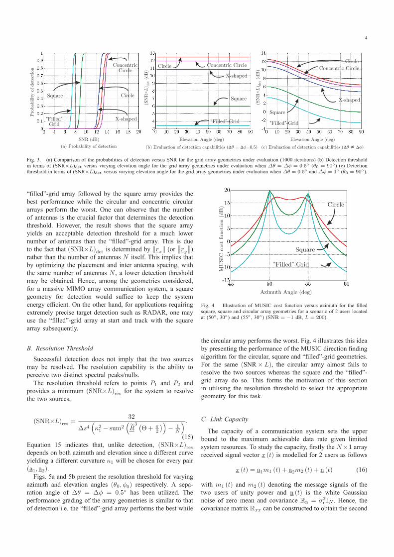
too. Fig. 3a illustrates the probability of detection versus vary-

ing SNR for two users with a fixed separation of 0.5 degrees

along the azimuth and elevation (∆θ = ∆φ = 0.5◦) and with

L = 200 snapshots across different grid geometries. In this

trial, the AIC (Akaike Information Criterion) [11] detection

algorithm has been employed and a detection iteration is

considered successful when the algorithm returns two users.

The results indicate that the best geometry is the “filled”-

grid array while the worst geometry is the circular array.

This illustrates the influence of array geometry in the task of

detection and the requirement to establish an accurate relation

between the detection threshold and the array geometry forms

the motivation of this section.

Figs. 3a and 3c illustrate the detection threshold presented

in Eq. 13 for the five grid array geometries under consid-

eration. The mid elevation angle φ0 = φ1+φ

2

2 is varied

while θ0 = (θ1+θ2)2 remains constant at 90

◦

. In Fig. 3b,

∆θ = ∆φ = 0.5◦, while in Fig. 3c, ∆θ = 0.5◦ and

∆φ = 1◦. As derived earlier, the detection threshold displays

a dependence on elevation when ∆θ 6= ∆φ. Please note thatthe simulation results with respect to varying azimuth are not

exhibited as the performance is constant with azimuth at all

times as predicted by Eq. 12. As reported by Table I, the

Performance Order Geometry

1st "Filled"-Grid

2nd Square

3rd X-Shaped

4th Concentric Circle

5th Circle

TABLE IPERFORMANCE RANKING OF ANTENNA ARRAY GEOMETRIES FOR THE

TASK OF DETECTION

4

SNR (dB) Elevation Angle (deg) Elevation Angle (deg)

(SN

R)

(dB

)×

det

(SN

R)

(dB

)×

det

(a) Probability of detection (b) Evaluation of detection capabilities ( = =0.5) (c) Evaluation of detection capabilities ( )

Pro

bability

ofdet

ecti

on

Square

Circle

X-shaped

“ ”Filled -Grid

Concentric Circle

Square

Circle

X-shaped

“ ”Filled -Grid

Concentric Circle

Square Circle

X-shaped“ ”FilledGrid

ConcentricCircle

Fig. 3. (a) Comparison of the probabilities of detection versus SNR for the grid array geometries under evaluation (1000 iterations) (b) Detection thresholdin terms of (SNR×L)det versus varying elevation angle for the grid array geometries under evaluation when ∆θ = ∆φ = 0.5◦ (θ0 = 90◦) (c) Detectionthreshold in terms of (SNR×L)det versus varying elevation angle for the grid array geometries under evaluation when ∆θ = 0.5

◦ and ∆φ = 1◦ (θ0 = 90◦).

“filled”-grid array followed by the square array provides the

best performance while the circular and concentric circular

arrays perform the worst. One can observe that the number

of antennas is the crucial factor that determines the detection

threshold. However, the result shows that the square array

yields an acceptable detection threshold for a much lower

number of antennas than the “filled”-grid array. This is due

to the fact that (SNR×L)det is determined by krxk (or ry )

rather than the number of antennas N itself. This implies that

by optimizing the placement and inter antenna spacing, with

the same number of antennas N , a lower detection threshold

may be obtained. Hence, among the geometries considered,

for a massive MIMO array communication system, a square

geometry for detection would suffice to keep the system

energy efficient. On the other hand, for applications requiring

extremely precise target detection such as RADAR, one may

use the “filled”-grid array at start and track with the square

array subsequently.

B. Resolution Threshold

Successful detection does not imply that the two sources

may be resolved. The resolution capability is the ability to

perceive two distinct spectral peaks/nulls.

The resolution threshold refers to points P1 and P2 and

provides a minimum (SNR×L)res for the system to resolve

the two sources,

(SNR×L)res =32

∆s4�κ21 − sum2

�eR3 �Θ+ π

2

��− 1

N

� .

(15)

Equation 15 indicates that, unlike detection, (SNR×L)resdepends on both azimuth and elevation since a different curve

yielding a different curvature κ1 will be chosen for every pair

(a1, a2).Figs. 5a and 5b present the resolution threshold for varying

azimuth and elevation angles (θ0, φ0) respectively. A sepa-

ration angle of ∆θ = ∆φ = 0.5◦ has been utilized. The

performance grading of the array geometries is similar to that

of detection i.e. the “filled”-grid array performs the best while

Azimuth Angle (deg)

MU

SIC

cost

funct

ion

(dB

)

Square

Circle

“ ”Filled -Grid

Fig. 4. Illustration of MUSIC cost function versus azimuth for the filledsquare, square and circular array geometries for a scenario of 2 users locatedat (50◦, 30◦) and (55◦, 30◦) (SNR = −1 dB, L = 200).

the circular array performs the worst. Fig. 4 illustrates this idea

by presenting the performance of the MUSIC direction finding

algorithm for the circular, square and “filled”-grid geometries.

For the same (SNR× L), the circular array almost fails to

resolve the two sources whereas the square and the “filled”-

grid array do so. This forms the motivation of this section

in utilising the resolution threshold to select the appropriate

geometry for this task.

C. Link Capacity

The capacity of a communication system sets the upper

bound to the maximum achievable data rate given limited

system resources. To study the capacity, firstly the N×1 arrayreceived signal vector x (t) is modelled for 2 users as follows

x (t) = a1m1 (t) + a2m2 (t) + n (t) (16)

with m1 (t) and m2 (t) denoting the message signals of the

two users of unity power and n (t) is the white Gaussian

noise of zero mean and covariance Rn = σ2nIN . Hence, the

covariance matrix Rxx can be constructed to obtain the second

5

(a) Resolution capabilities against azimuth (b) Resolution capabilities against elevation

(SN

R)

(dB

)×

res

(SN

R)

(dB

)×

res

Azimuth Angle (deg) Elevation Angle (deg)

Square

Circle

X-shaped

“ ”Filled -Grid

Concentric Circle

Square

Circle

Xshaped

“ ”FilledGrid

ConcentricCircle

Fig. 5. (a) Resolution threshold in terms of (SNR×L)res versus varying azimuth angle for the array geometries under evaluation (φ0 = 40◦) (b) Resolution

threshold in terms of (SNR×L)res versus varying elevation angle for the array geometries under evaluation (θ0 = 80◦).

order statistics of x(t) as

Rxx = Enx (t)x (t)

Ho

=

Rdesiredz }| {a1a

H1 +

Rundesiredz }| {a2a

H2 + 2Re

�ρ12a1a

H2

+

Rnz}|{σ2nIn, (17)

where Rdesired is the covariance matrix of user 1 and

Rundesired contains the covariance matrices of user 2 and the

term arising from ρ, the cross-correlation coefficient of the

messages transmitted by users 1 and 2. Also, Rn is the noise

covariance matrix. To receive the message of user 1, one can

steer a beam towards (θ1, φ1) by employing the manifold

vector a1 as a weight vector w (steering vector). In this case,

the system capacity can be characterized by the signal-to-noise

plus interference ratio at the output of the receiver, SNIRout,

as

C

B= log2 (1 + SNIRout)

= log2

�1 +

wHR1w

wH (R2 + Rn)w

�

= log2

1 +

aH1 a1aH1 a1

aH1 a2aH2 a1 + 2ρN Re

�aH2 a1

+ σ2na

H1 a1

!

= log2

1 +

N2

��aH1 a2��2 + 2ρN Re

�aH2 a1

+ σ2nN

!,

(18)

since aH1 a1 = N . Utilising the fact that the manifold of the

grid array lies on an N dimensional hypersphere and using

the length of the arc of the geodesic curve between P1 and

P2 in Fig. 1 given by Eq. 12, the inner product aH1 a2 can be

written as

aH1 a2 = N cos

�∆s√N

�(19)

= N cos

π krxk

p∆θ2 cos2 φ+∆φ2 sin2 φ√

N

!.

Using Eq. 19 and assuming ∆θ = ∆φ, Eq. 18 can be written

as

C

B= log2

1 +

N2

N2 cos2�πkrxk∆θ√

N

�+ σ2nN

. (20)

Without any loss of generality, it has been assumed that ρ = 0,implying that the messages transmitted by users 1 and 2 are

uncorrelated. Eq. 20 reveals a trade-off between the norm of

the geometry krxk (or equivalently ry for 2D-grid arrays)

and the number of antennas N . Hence, different geometries

will present different capacities with magnitudes depending on

an inverse cosine function of krxk ( or ry ), ∆θ (or ∆φ)

and the number of antennas N . Hence, there exists a trade-off

between the number of antennas in the array and the antenna

array geometry.

To illustrate this property, we present in Figs. 6a and 6b,

the evaluation of the capacity for the five geometries of Fig. 2

with varying elevation and constant azimuth θ = 90◦ (Fig. 6a),and varying azimuth for constant elevation φ = 50◦ (Fig. 6b).Please note that ∆φ = ∆θ = 3◦ and SNRin = 20 dB. Acrossall geometries, as shown in Figs. 6a and 6b, the square antenna

array exhibits the best performance with a maximum capacity

of 1.39 bits/sec/Hz achieved at θ̃ = 130◦ and φ̃ = 90◦.The square, circular and X-shaped antenna arrays surprisingly

outperform the “filled”-grid array which possesses the highest

number of antenna elements. This is inline with the result that

the “filled”-grid array has a poor ratio of cos−2�πkrxk∆θ√

N

�

while the square array yields the highest ratio closely followed

by the circular array. A higher ratio of this key term implies

higher capacity according to Eq. 20.

Apart from the common perception that the capacity de-

pends solely on the number of antennas, this study illustrates

that the capacity depends mainly on the particular array. Thus,

the square array of 40 antennas, for instance, has higher

capacity and better energy efficiency than a “filled”-grid array

with more (121) antennas. However, the “filled”-grid array has

better resolution and detection capabilities.

6

Azimuth Angle (deg) Elevation Angle (deg)

Capaci

ty(b

its/

sec/

Hz)

Capaci

ty(b

its/

sec/

Hz)

(b) Evaluation of capacity against elevation

Square Square

CircleCircle

X-shaped X-shaped

“ ”Filled -Grid“ ”Filled -Grid

Concentric Circle Concentric Circle

Fig. 6. Steering vector beamformer for the array geometries shown in Fig. 1: (a) Capacity (bits/sec/Hz) versus azimuth angle for the array geometriesunder evaluation (φ0 = 50◦, ∆θ = ∆φ = 3◦) (b) Capacity (bits/sec/Hz) versus elevation angle for the array geometries under evaluation (θ0 = 90◦,∆θ = ∆φ = 3◦). In both cases, the input SNR was chosen to be 20dB.

V. CONCLUSION

In this paper, various grid array geometries for different ap-

plications have been studied and compared by employing rele-

vant performance criteria as figures–of–merit. Five geometries

were examined by picking subsets of antennas from a 11×11“filled”-grid array and their performance were evaluated in the

context of a multi-user system where two cochannel users are

located close together in space. As a next step, the performance

of the system may be further improved by selecting antenna

elements dynamically. Hence, for upcoming 5G systems that

are to span a variety of applications, selection of appropriate

array geometry as per the task at hand is a crucial tool to

exploit.

REFERENCES

[1] D. Sadler and A. Manikas, “Blind reception of multicarrier ds-cdmausing antenna arrays,” IEEE Transactions on Wireless Communications,vol. 2, pp. 1231–1239, Nov. 2003.

[2] X. Huang, Y. J. Guo, and J. D. Bunton, “A hybrid adaptive antenna ar-ray,” IEEE Transactions on Wireless Communications, vol. 9, pp. 1770–1779, May 2010.

[3] J. Nsenga, A. Bourdoux, and F. Horlin, “Mixed analog/digital beam-forming for 60 GHz mimo frequency selective channels,” in IEEEInternational Conference on Communications, pp. 1–6, May 2010.

[4] U. Baysal and R. Moses, “On the geometry of isotropic arrays,” IEEETransactions on Signal Processing, vol. 51, pp. 1469–1478, June 2003.

[5] M. Gavish and A. Weiss, “Array geometry for ambiguity resolution indirection finding,” IEEE Transactions on Antennas and Propagation,vol. 44, pp. 889–895, June 1996.

[6] J.-W. Liang and J. Paulraj, “On optimizing base station antenna arraytopology for coverage extension in cellular radio networks,” in IEEEVehicular Technology Conference, pp. 866–870, July 1995.

[7] J. S. Petko and D. H. Werner, “Interleaved ultrawideband antenna arraysbased on optimized polyfractal tree structures,” IEEE Transactions onAntennas and Propagation, vol. 57, pp. 2622–2632, Sept. 2009.

[8] A. Manikas, A. Alexiou, and H. Karimi, “Comparison of the ultimatedirection-finding capabilities of a number of planar array geometries,”IEE Proceedings - Radar, Sonar and Navigation, vol. 144, pp. 321–329,Dec. 1997.

[9] N. Dowlut and A. Manikas, “A polynomial rooting approach to super-resolution,” IEEE Transactions on Signal Processing, vol. 48, pp. 1559–1569, June 2000.

[10] A. Manikas, Differential Geometry in Array Processing. London:Imperial College Press, 2004.

[11] H. Akaike, “A new look at the statistical model identification,” IEEETransactions on Automatic Control, vol. 19, pp. 716–723, Dec. 1974.