POLYMER SCIENCE

FUNDAMENTALS OF POLYMER SCIENCE

Molecular Weights of Polymers

Prof. Premamoy GhoshPolymer Study Centre

“Arghya” 3, Kabi Mohitlal RoadP.P. Haltu, Kolkata- 700078

(21.09.2006)

CONTENTSIntroductionConcept of Average Molecular WeightNumber Average Molecular WeightMembrane OsmometryWeight Average Molecular WeightAssessment of Shape of Polymer MoleculesViscosity Average Molecular WeightGeneral Expression for Viscosity Average Molecular WeightZ-Average Molecular WeightGeneral Requirement for Extrapolation to Infinite DilutionPolymer Fraction and Molecular Weight DistributionGel Permeation ChromatographyMolecular Size parameterPolymer End Groups and End Group Analysis

Key Words

Number average, weight average, viscosity average, z-average, osmometry,light scattering, turbidity, dissymmetry, size and shape, semipermeablemembrane, osmotic pressure, viscometry, solution viscosity, intrinsicviscosity, infinite dilution, sedimentation, fractionation, molecularweight distribution, distribution ratio / polydispersity index, endgroup, gel permeation chromatography, hydrodynamic volume, dyetechniques, refractive index.

IntroductionFor many reasons, particularly to know more about polymermolecular systems, it is necessary to characterize them withrespect to (i) the chemical identity of their repeat units,(ii) nature of end groups present, (iii) existence ofbranching with nature of branch units and their frequency,(iv) presence of comonomer units and also copolymercomposition and comonomer sequence distribution in copolymersystems, (v) solubility and associated features, (vi)optical properties covering clarity or degree of clarity andrefractive index, and (vii) resistance properties withreference to thermal, mechanical and electrical resistances,photoresistance or photostability, chemical and weatherresistance, corrosion resistance, and also bioresistance orresistance to biodegradation. But what is more importantand fundamental is knowledge about the molecular weight of agiven polymer. For molecular weight determination, it isnecessary to dissolve the polymer in an appropriate solventand begin with a dilute solution.

Concept of Average Molecular Weight A specified polymer material is generally a mixture ofmolecules of identical or near – identical chemicalstructure and composition, but differing in degree ofpolymerization (DP) or molecular weight. The moleculesproduced by polymerization reaction have chain lengths thatare distributed according to a probability function that isgoverned by the polymerization mechanism and by thecondition prevailing during the process. A concept of

average molecular weight, therefore, assumes importance andvery much relevant. However, assignment of a numericalvalue to the molecular weight will be dependent on thedefinition of a particular average. An average molecularweight, M may in fact be generally expressed as

M = f1 M1 + f2 M2 + f3 M3 + ------ = Σ fi Mi (1)

Here, M1 , M2 , M3 etc. refer to molecular weights ofdifferent sizes of molecules and the coefficients f1 , f2 , f3

etc. are fractions such that their summation Σ fi equals tounity. The average molecular weight M may otherwise beexpressed as

Σ Ni Mi a

M = (2)Σ Ni Mi

(a – 1)

where, Ni is the number of molecules, each of which ischaracterized by the molecular weight Mi and the index ‘a’may have any real value. Two very important averagemolecular weight widely recognized and used are (i) numberaverage molecular weight, Mn and (ii) weight averagemolecular weight, Mw. Setting a = 1 in equation (2), oneobtains the expression for the number average molecularweight, Mn :

Σ Ni Mi

Mn = (3) Σ Ni

Equation (3) can, in fact, be expressed as a simplesummation series resembling equation (1) where thefractional coefficients are actually the mole fractions ofthe respective molecular species existing in the polymersystem such that total weight W = Σ Ni Mi and total numberof molecules N = Σ Ni , Thus,

W Σ Ni Mi N1 N2 N3

Mn = = = M1 + M2 + M3 + ------ N Σ Ni N N N

= f1 M1 + f2 M2 + f3 M3 + ------- (4)

On the other hand, however, setting a = 2 in equation (2),

one finds the expression for weight average molecular

weight, Mw , i.e.,

Σ Ni Mi 2

Mw = (5) Σ Ni Mi

Equation (5) can also be rearranged and expressed as asummation series as given by equation (1), but in this case,the fractional coefficients actually correspond to weightfractions of different molecular species present. So, onemay write :

Σ Ni Mi . Mi Σ wi Mi

Σ wi Mi

Mw = = = Σ Ni Mi Σ wi W

w1 w2 w3

= M1 + M2 + M3 + ------ W W W

= f1 M1 + f2 M2 + f3 M3 + -------

(6)

Here, w1 , w2 , w3 , etc. stand for weight of differentmolecular species having molecular weight M1 , M2 , M3 etc.respectively and Σ wi = W gives the total weight of all themolecules present.

The obvious consequences of above definitions imply that Mw

≥ Mn , i.e., Mw / Mn 1; ≥ the equality, however, relates to aperfectly monodisperse polymer sample where all the polymermolecules are of equal molecular weight, i.e. M1 = M2 = M3 =

----- = M. So, for monodisperse systems, (Mw / Mn) = 1.Deviation from unity of the ratio Mw / Mn , known as thedistribution ratio is taken as a measure of polydispersityof the polymer sample. The said ratio is also referred to aspolydispersity index; a higher value of the ratio means agreater polydispersity.

Evaluation of number average molecular weight is helpful forhaving a good understanding of polymerization mechanism andrelevant kinetics. Mn is useful in the analysis of kineticdata and assessing or ascertaining effects of many sidereactions such as chain transfer, inhibition and retardationand also autoacceleration effects during vinyl and relatedpolymerizations. The number average molecular weightassumes prime importance in the context of studies ofsolution properties that go by the name of colligativeproperties viz., vapour pressure lowering, freezing pointdepression, boiling point evaluation and osmometry. Polymermolecules of lower molecular weight or even low molecularweight soluble impurities contribute equally and enjoy equalstatus with polymer molecules of higher molecular weights indetermining the colligative properties.

On the other hand, weight average molecular weight assumesimportance in the context of various bulk properties ofpolymers, particularly the rheological and resistanceproperties. Softening/melting and hot deformation, melt –viscosity or melt – flow, tensile and compressive strength,elastic modulus and elongation at break, toughness andimpact resistance and some other bulk properties of polymersare better appreciated on the basis of weight averagemolecular weight, keeping in mind, however, the influence ofchemical nature of the repeat units, degree of branching andcross linking, thermal or thermomechanical history of thepolymer sample, etc.

Number Average Molecular Weight Number average molecular weight can be evaluated usingdilute solution of a polymer making use of ebulliometric

(boiling point elevation), cryoscopic (freezing pointdepression) and osmometric (membrane osmometry)measurements.Direct measurements of vapour pressure loweringof dilute polymer solution lack precision and mostly produceuncertain results. Vapour – phase osmometry, however, allowsindirect exploitation of vapour pressure lowering of polymersolution at equilibrium as can be related through theClapeyron equation and in this method, one measures atemperature difference that can be related to vapourpressure lowering. This difference in temperature iscomparable to or of the same order of magnitude as thoseobserved in cryoscopy and ebulliomtry. These methodsrequire calibration with low molecular weight standards andthey may produce reliable results for polymer molecularweights < 30,000. The working equations for ebulliometric,cryoscopic and osmometric measurements are as follows:

T∆ b RT 2 1lim = . (7)c o→ c ρ H∆ ν M

T∆ f RT 2 1lim = . (8)c o→ c ρ H∆ f M

π RT lim = (9)c o→ c M

where, T∆ b , T∆ f , and π are boiling point elevation, freezingpoint depression and osmotic pressure, ρ is the density ofthe solvent, H∆ ν and H∆ f are respectively the latent heatof vaporization and of fusion of the solvent per gram, c isthe polymer (solute) concentration in g/cm3 and M is thesolute molecular weight. Very low observed temperaturedifferences (of the order of 10-3 0C) for low finiteconcentrations of a polymer of the molecular weight range of≥ 20,000 and lack of development of equipments forebulliometric and cryoscopic measurements have turned them

unattractive and less useful. Vapour pressure lowering forlow finite concentrations is also very low (of the order of10-3 mm Hg) for such polymers. The osmotic method is inmore wide use than other colligative techniques as becausethe osmotic response is of a magnitude that is easilyobservable and measurable, even though success of thismethod is contingent upon availability of prefect osmoticmembranes.

Membrane Osmometry Let us take the case of a dilute polymer solution of a lowfinite concentration separated from the pure solvent by asemipermeable membrane. The chemical potential of thesolvent (μs) in solution is lees than that (μo) of puresolvent and therefore, to keep the system in equilibrium,the chemical potential of the solvent on the two sides ofthe membrane requires to be balanced and made equal. Thisis readily done by applying an excess pressure, π , calledthe osmotic pressure to the solution side to compensate forthe difference in chemical potential. The equilibriumcondition can thus be expressed as :

μo – μs = μ∆ 1 = – π V1

Or, RT ln f1 x1 = – π V1 (10)

where, R is the universal gas constant, T, the absolutetemperature, V1, the partial molar volume, f1, the activitycoefficient of the solvent in solution, and x1, the solventmole fraction; for a very dilute solution, f1 → 1 and V1 maybe taken as equal to the molar volume V1

0 of the pure

solvent. Replacing solvent mole fraction x1 by (1 – x2),where x2 is the mole fraction of the (polymer) solute insolution, and expanding the logarithm factor, one obtains

x22 x2

3

π V10 = RT x2 + + + ------ (11)

2 3

If c is the concentration of the solute in gram per unitvolume of the solution, then for a very low value of c andvery high value of Mn , x2 is given by

c / Mn V1 0 c

x2 = ~ (12) 1/ V1

0 + c / Mn Mn

Combining equation (11) and (12), one obtains

RT 1 V10 1 V1

0 2

π / c = 1 + c + c2+-----(13)

Mn 2 Mn 3 Mn

Polymer solutions largely deviate from ideality, thusrendering the value of f1 less than unity; even at a verylow finite concentration at which precision osmometricmeasurement is possible. The real coefficients ofconcentration terms in equation (13) are somewhat higherthan those shown in the equation. Even then, the π / c termmay be expressed as a power series in c using empiricalcoefficients :

π / c = RT ( A1 + A2 c + A3 c 2 + ----- ) (14)

Or alternatively, RT

π / c = ( 1 + Г2 c + Г3 c 2 + ----- ) (15) Mn

where, Г2 = A2 / A1 , Г3 = A3 / A1 and so on, and A1 = ( 1 / Mn )

The coefficient A2, A3 etc. are referred to as second, third,etc. virial coefficients. For most cases and for allpractical purposes, the term in c 2 and those in higherpowers of c may be neglected. Thus, π / c is measured as afunction of c in unit of g/dl at a given temperature andplotted graphically; extrapolation of the low concentrationrange linear plot with a positive slope to c o→ gives anintercept that equals the parameter (RT / Mn).

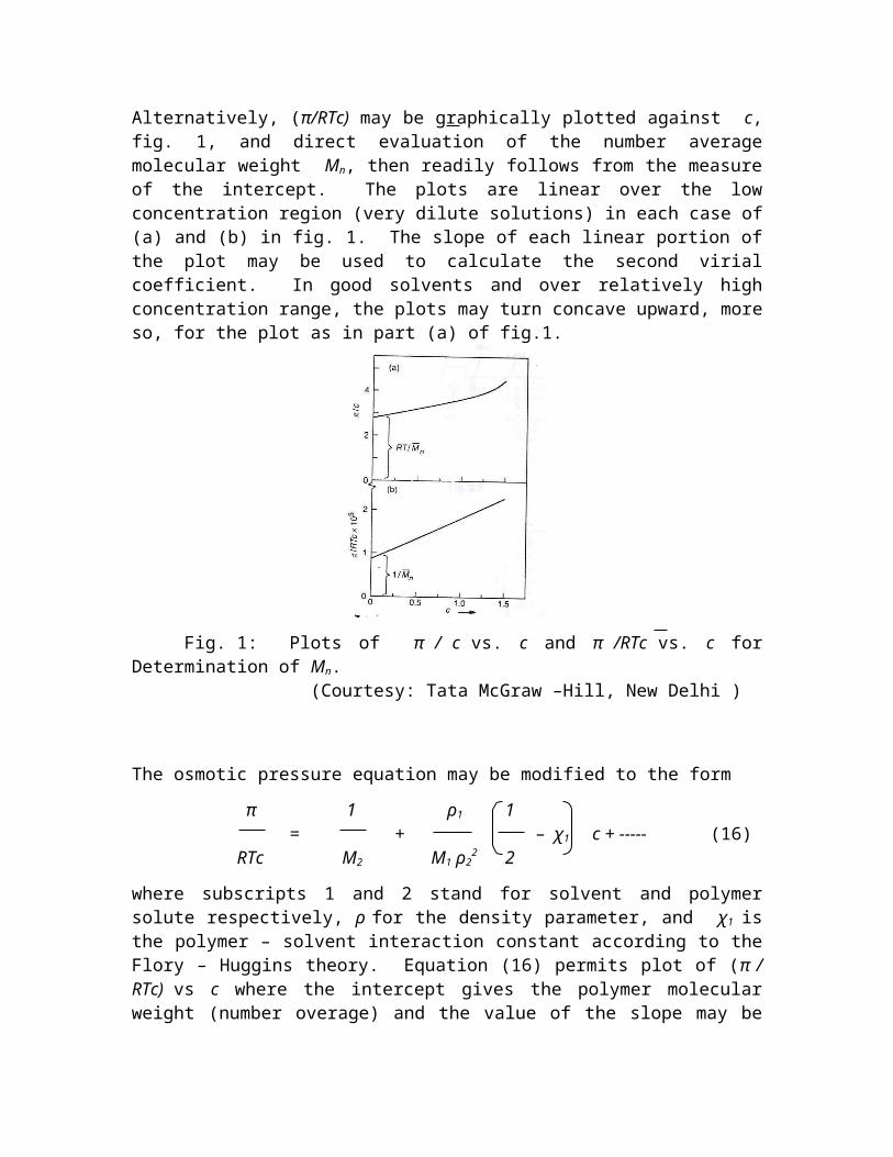
Alternatively, (π/RTc) may be graphically plotted against c,fig. 1, and direct evaluation of the number averagemolecular weight Mn, then readily follows from the measureof the intercept. The plots are linear over the lowconcentration region (very dilute solutions) in each case of(a) and (b) in fig. 1. The slope of each linear portion ofthe plot may be used to calculate the second virialcoefficient. In good solvents and over relatively highconcentration range, the plots may turn concave upward, moreso, for the plot as in part (a) of fig.1.

Fig. 1: Plots of π / c vs. c and π /RTc vs. c forDetermination of Mn.

(Courtesy: Tata McGraw –Hill, New Delhi )

The osmotic pressure equation may be modified to the form

π 1 ρ1 1= + – χ1 c + ----- (16)

RTc M2 M1 ρ22 2

where subscripts 1 and 2 stand for solvent and polymersolute respectively, ρ for the density parameter, and χ1 isthe polymer – solvent interaction constant according to theFlory – Huggins theory. Equation (16) permits plot of (π /RTc) vs c where the intercept gives the polymer molecularweight (number overage) and the value of the slope may be

used to calculate the value of Flory – Huggins polymer –solvent interaction constant χ1.

Both slope and curvature are zero at θ temperature. Themembrane osmometry is based on the principle described infig. 2. The membrane used is of critical importance. Itshould permit the small solvent molecules to permeatethrough but would be non permeable to even the smallestmacromolecules present in the test polymer sample. So, themembrane is better called semipermeable. All measurementsin a specific case must necessarily be made at a specifiedand constant temperature, preferably using the samesemipermeable membrane too. The thermodynamic drive toreach equilibrium causes entry of (more) solvent moleculesfrom the solvent chamber to the solution side, therebycausing the liquid level in the solution side to rise tillthe hydrostatic pressure on the membrane on the solutionside balances the osmotic pressure on the same in thesolvent side. Use of a narrow capillary over each of thesolution and solvent chambers makes it easy to follow therise in liquid height on the solution side and finally tomeasure the difference in liquid heights on the two sides onattainment of the equilibrium. The difference in liquidlevels at equilibrium is used to calculate the osmoticpressure.

Fig. 2: Operating Principle and Schematic Presentation ofa Membrane Osmometer

(Courtesy: Tata McGraw –Hill, New Delhi )

Membranes based on cellulose such as regenerated cellulose(gel cellophane) are most widely used. Other suitablemembrane materials are collodion (nitrocellulose, 11 – 13%N2) and denitrated collodion, poly(vinyl alcohol),poly(vinyl butyral), etc. Osmometer cell and assemblyaccording to Zimm and Meyerson, and shown in fig. 3, is morepopular for its simplicity. Time periods required forattainment of equilibrium in classical osmometers usingdilute polymer solutions range on the average between 10 –25 h.

Fig. 3: Sections and Parts of a Zimm – Meyerson Osmometer(Courtesy: Tata McGraw –Hill, New Delhi )

Different models of high–speed osmometers have beendeveloped. Most of them feature a closed solvent chambergadgeted with a sensitive pressure-sensing device withoutthe use of a capillary. Such equipments use suitablephotoelectric or other devices for sensing pressure orpressure difference employing a servomechanism or else,using a strain gauge. The high-speed equipments permitattainment of equilibrium within 5 min.

Weight Average Molecular Weight: Light Scattering By PolymerSolutions

The subject of scattering of light by gaseous systems(Rayleigh scattering) or by colloidal system suspended in a

liquid medium (Tyndal scattering) has been widely studied.The intensity of scattered light depends on thepolarizability of the molecules or particles compared withthat of the surrounding medium in which they exist, i.e.dissolved, mixed or suspended. It further depends on themolecular or particle size and on their concentration. Ifthe homogeneous mixture, solution or dispersion issufficiently dilute, the intensity of the scattered light isequal to the sum of the contributions from the individualmolecules / particles, each being unaffected by the othersin the medium.

Let us now consider a beam of light passing through anoptically inhomogeneous medium of path length, l is beingscattered in all directions; The intensity of thetransmitted beam I decreases exponentially and is related tothat Io of the incident beam and the relationship may beexpressed as,

I = Io e – τ l (17)

Here, the parameter τ is referred to as turbidity. Let ustake the case of a polymer solution. Thermal agitation ofthe molecules in solution causes instantaneous localfluctuation of density and concentration. For differentpolarizabilities of solute and solvent, the intensity oflight scattered by a tiny volume element also varies withsuch fluctuations arbitrarily on a continuous basis. Theeffect arising from density fluctuations can be accountedfor by subtracting the intensity of the light scattered bythe pure solvent from that scattered by the solution. The work expended to produce a given concentrationfluctuation is related directly to the free energy ofdilution, G∆ 1. So, the scattered light intensity can be usedto measure the thermodynamic properties. The scatteredlight intensity from a solution is commonly expressed interms of its turbidity τ , which is the fraction by whichthe scattered beam is reduced over 1 cm path length ofsolution according to equation (17). For polymer molecules

of size smaller than the wave length of light used, τ isexpressed as :

32 π 3 k T n2 c ( n / c )∂ ∂ 2 V1

τ = (18) 3 λ4 (– G∂ ∆ 1 / c )∂

Here, k is Boltzmann’s constant, n the refractive indexof the medium, ( n / c )∂ ∂ , the change in refractive index withconcentration, c, λ, the wave length of the incident beam and

G∆ 1 signifies the difference between the molar free energyof the pure solvent and partial molar free energy of thesolvent in solution of concentration c. Now, having therelation G∆ 1 = – π V1 based on equation (10), where π is theosmotic pressure and using the relation between π andmolecular weight, one may logically write.

RT V1

– ( G∂ ∆ 1 / c) =∂ ( 1 + Г2 c + ….) (19) M

Combining equations (18) and (19), one may derive

H (c / τ) = (1/M) ( 1 + Г2 c + ….) (20)

where, H = (32 π 3 n2 / 3 λ4 No) ( n / c )∂ ∂ 2 , is a constant for agiven solute – solvent system. and No = R/k is theArogadro’s number. If τ is determined as a function of c andH(c / τ) is plotted against c, then the intercept on the H(c / τ)axis as obtained on extrapolation of the straight line plotto zero concentration or more appropriately to infinitedilution, fig. 4, permits ready calculation of the molecularweight M, which for a polydisperse polymer solute, can beshown to be the weight average molecular weight Mw.

Fig. 4 : A Typical Linear Plot of Hc/τ vs. c forDetermination of Mw

(Courtesy: Tata McGraw –Hill, New Delhi ) Light scattering photometers employ photoelectric techniquefor measurements of scattering data. The measurementprinciple and approach is a simple one and is outlined infig.5. It is absolutely important and necessary that themeasuring chamber, and the solvent and solutions are keptdirt or dust free. The specified scattering glass – cell isplaced on the fixed center – table and centred on the axisof rotation of the receiver photomultiplier tube assembly;this assembly can be rotated and fixed at desired angularpositions for measurements of the scattered light. Besidesthe measurements of intensities of incident and scatteredlight, i.e. the turbidity. τ , it is necessary to determinethe refractive index n of solvent and the parameter( n / c) ∂ ∂ using a differential refractometer. The choice ofsolvent is also important. The difference in the refractiveindex between the polymer and the solvent should be as largeas possible. A solvent of low second virial coefficientmakes a more precise evaluation of Mw possible by the usualmethod of extrapolation to infinite dilution condition, i.e.to zero concentration. Molecular weights ranging from10,000 to 10,000,000 are measurable by this technique.

Fig. 5: Operating Line and Principle of Light ScatteringPhotometer

(Courtesy: Tata McGraw –Hill, New Delhi)Assessment of Shape of Polymer MoleculesFor polymer molecules much smaller than the wave length ( λ) of the incident light, the scatterings in the forward andbackward directions measured at two angles symmetrical about900 (say 450 and 1350) are not appreciably different. Butfor particles larger than about a tenth of the wavelength oflight, the scattered light intensity follows a loweringtrend from front to rear. The intensity ratio (i45° / i135°),known as dissymmetry (Z) of light scattering is unity forsmall particles and its value increases with increase insize of homogeneously mixed, dispersed or dissolvedparticles. Evaluation of the dissymmetry may beadvantageously used to estimate particle size, which is theeffective expanse of the particle. If the particle weightis also determined or known, then the measure of dissymmetrygives an idea about the shape of the particles as to whetherthey are characteristically spherical, disc-like, rod-likeor random coils. There are, however, some intrinsiclimitations to this approach of particle shapedetermination.

Methods of average molecular weight determination of a givenpolymer sample by membrane osmometry (giving Mn) and lightscattering (giving Mw) are viewed as absolute methods, andthe ratio Mw / Mn can then be used to get an idea about thedistribution ratio or poly dispersity index of the polymerstudied.

Viscosity Average Molecular Weight The viscosity of a polymer solution ( η ) is higher thanthat ( ηo ) of the pure solvent at a specified temperatureand the increase in medium viscosity on dissolving thepolymer in the solvent is a function of both molecularweight and concentration of the polymer solute. Thesolution viscosity can be measured easily; it however, fallsfar short of giving a direct and absolute value of polymermolecular weight.

Despite this shortcoming, viscometry has emerged as a usefuland simple technique in the context of having a measure ofpolymer molecular weight. If the polymer solution is verydilute and as a result, the change in density due to thedissolved polymer is negligible, then the viscosities of thesolvent and the solution at a given temperature would beproportional to their flow times in a given capillaryviscometer such that the relative viscosity, ηr expressedby the ratio, (η / ηo) would be given by the flow time ratio(t / to), where to is the flow time of a given volume of thesolvent and t is the flow time of the same volume ofsolution respectively. The parameter called specificviscosity, ηsp as defined by ηsp = (η – ηo) / ηo = (t –to) / to as well as the relative viscosity (ηr) aredimensionless.

If the solute polymer molecules do not interfere with oneanother during flow through the fine capillary of theviscometer, then the increase in viscosity due to thepresence of the dissolved polymer molecules is proportionalto their concentration and the parameter ηsp / c, called thereduced viscosity would be theoretically expected to be aconstant. In reality, however, for most polymer – solventsystems, ηsp / c is generally found to increase withincrease in the value of c, as in fig. 6. For dilutepolymer solutions, a plot of ηsp / c vs. c is usually astraight line with a positive slope. The viscometricparameter called the intrinsic viscosity or the limitingviscosity number, [η] for a given polymer – solvent system

at a given temperature is given by the intercept of thelinear plot of ηsp / c vs. c i.e. by extrapolation of theplot (fig. 6) to a condition of zero concentration, or moreprecisely to infinite dilution condition and the viscosityaverage molecular weight (Mν) is given by the semi empiricalMark – Houwink equation :

Lt . c o , η → sp / c = [η] = K Mν a (21)

Fig. 6 : Viscometric Plots ( η sp / c ) vs. c and ( ln ηr / c ) vs. c(Courtesy: Tata McGraw –Hill, New Delhi )

where K and a are known as Mark Houwink constants for aparticular polymer – solvent system at the giventemperature. ηsp / c at finite concentration may beexpressed as a function of [η] and the relevant expressionis known as Huggins’ equation.

( ηsp / c ) = [η] + k1 [η] 2 c (22)

Another useful equation known as Kraemer’s equation runs as

follows:

( ln ηr )/ c = [η] + k2 [η] 2 c (23)

The term ( ln ηr )/ c is commonly referred to as the inherentviscosity. The reduced viscosity, inherent viscosity andintrinsic viscosity are commonly expressed in the unit of

reciprocal concentration, i.e. decilitre per gram (dl / g), cbeing commonly expressed as g / dl or g/100 cc. The constantsk1 and k2 of equations (22) and 23) are known as Huggins’constant and Kraemer’s constant respectively. For mostcases k2 is negative and it is the general experience that k1

– k2 = 0.5. The slope of each plot, left hand side vs. c foreach of Huggins’ equation and Kraemer’s equation isproportional to [η]2 and the two plots made using commonordinate and abscissa would extrapolate to a common point onthe ordinate. One can thus get a precise [η] value based onsuch duel plots as in fig. 6.

Each of the above two equations provides a basis fordetermination of polymer molecular weight from viscometricmeasurements. The value of Mν thus obtained is not anabsolute value in view of incomplete interpretations of Kand a values (equation (21)).

One has to determine the K and a values by measuring the[η] values of monodisperse polymer samples whose molecularweights have been obtained from, one of the absolute methodssuch as osmometry (giving Mn ) and light scattering(giving Mw ) and making use of respective plot of log [η]vs. log M, which is a straight line plot. The value ofthe constant, a (exponent of molecular weight in equation(21)) is obtained from the slope of the plot, fig. 7. Thevalue of the exponent a usually varies between 0.5 and0.8. It does not fall below 0.5 normally and it may exceed0.8 in rare cases, particularly for solutions ofpolyelectrolytes bearing no added salt.

Fig. 7 : Logarithmic Plot of [ η ] vs. M (Schematic).(Courtesy: Tata McGraw –Hill, New Delhi )

K and a are best understood for nearly all systems if [η]is determined at the theta (θ) temperature, when a =0.5 ; K depends on the measuring temperature whileremaining independent of solvent, keeping in mind of coursethat the solvent fixes the temperature of measurement. Atthe θ temperature, the change in solvent chemical potentialdue to interaction with the segments of the polymer soluteis zero, and the deviations from ideality just vanish. So,the free energy of interactions of solute segments within avolume element is zero. θ temperature is in fact thelowest temperature for complete miscibility of the solute inthe poor solvent used at the theoretical limit of infinitemolecular weight. The ideality is attained at T = θ in viewof the position that chain molecular dimensions areunperturbed by intramolecular interactions.

General Expression for Viscosity Average Molecular Weight At infinite dilution (c o→ ), the polymer molecules insolution contribute to viscosity discretely without mutualinterference. Solubilization of a polymer sample ispreceded by a large amount of swelling if left undisturbedand the swelling degree is higher in a better solvent.Similarly, the intrinsic viscosity is also higher in a goodsolvent than in a poor solvent. What all these would meanis that in a better solvent, as the polymer chain moleculesgo into solution, a unit mass of the same expands more togive a higher hydrodynamic volume.

Let there be a heterogeneous (polydisperse) polymer indilute solution of concentration c considered to behaveideally in that the individual molecules contribute toviscosity enhancement independently of one another. In thatevent, if ( ηsp ) i be the specific viscosity contribution

due to the species of size i , then one may express theoverall specific viscosity ηsp as ηsp = Σ (ηsp ) i

(24)

Considering Mi and ci as the molecular weight andconcentration of the species of size i and in view of theideal specific viscosity component ( ηsp )i = KMi

a ci , it isfurther possible to write.

ηsp = K Σ Mi a ci (25)

and so, ( ηsp / c ) = [η] = ( K Σ Mi

a ci ) / c(26)

where, c = Σ ci stands for overall concentration taking allpolymer species into consideration. Further taking c = Σ ci

= Σ Ni Mi , and considering the (Mark Houwink) equation (21),one may have :

Σ Ni Mi (1 + a)

[η] = K = K Mν a (27)

Σ Ni Mi

such that, Σ Ni Mi

(1 + a) 1/a

Mν = (28) Σ Ni Mi

Clearly, one may see that for the limiting case when a =

1 , Mν = Mw

The viscometric studies as a means of molecularcharacterization of polymers are recognized to be verysimple in respect of experimental approach and apparatusneeded and hence, widely practiced. Dilute solutionviscosity is very easily measured using capillaryviscometers of the Ostwald type or the Ubbelohde type, fig.8. The Ubbelohde type is a suspended level dilutionviscometer having the advantage that the flow time measuredis independent of the volume of liquid (for solvent andsolutions) in the viscometer; measurements at a series of

concentrations can be conveniently done by successivedilution within the viscometer itself. All flow timemeasurements for solvent and solutions of differentconcentration or dilution are carried out in a thermostatedbath regulated within + 0.1 0C. The flow time data are thenplotted graphically using equation (22) and/or (23) and thenextrapolated to infinite dilution ( c o→ ) to obtain thevalue of [η] or the intrinsic viscosity, as has beendescribed earlier in this chapter. Mv is then calculatedout using the Mark – Houwink equation and taking help ofappropriate K and a values from the literature, ifavailable, or from an independent determination as describedearlier.

Fig. 8 : (a) Ostwald – type and (b) Ubbelohde – typeCapillary Viscometers

(Courtesy: Tata McGraw –Hill, New Delhi )

Z-Average Molecular Weight ( Mz )

The Z – average molecular weight, Mz is expressed as :

Σ Ni Mi 3

Mz = (29) Σ Ni Mi

2

For a given molecular weight distribution, the variousaverage molecular weights come in the order Mn < Mv < Mw

< Mz . The Z-average molecular weight is commonly measuredby sedimentation equilibrium method using anultracentrifuge.

The ultra centrifugation techniques are somewhat complicatedand much less commonly employed for molecular weightmeasurements of synthetic polymers, even though, they aremore commonly used for characterizing biological polymerssuch as proteins and enzymes. Employing a low speed of rotation with the polymer solutionin the cell held in position and operating theultracentrifuge under constant conditions for a long periodavoiding convection related disturbances within the cell, astate of equilibrium is reached. Under equilibriumcondition, the polymer fractions get distributed in the cellaccording to size or molecular weight distribution. Theforce of sedimentation on a molecular species in solution isjust balanced by its tendency to diffuse out. For dilutesolutions closely approaching ideal behaviour and for amonodisperse polymer, the molecular weight M is expressed as

2 RT ln ( c2 / c1 )M = (30)

(1 – v ρ) ω2 (r22 – r1

2)

where c1 and c2 are the concentration at two pointscorresponding to distances r1 and r2 in the cell and ωis the angular velocity of rotation, v, the partial specificvolume of the polymer and ρ, the density of the medium. Thesolvent chosen should be preferably a poor solvent having adensity far different from that of the polymer so as tofacilitate sedimentation; the solvent and polymer must alsodiffer in refractive index so as to facilitate easymeasurement. For a poly disperse polymer, differentapproaches for measuring the concentration as a function ofr yield different molecular weight averages ( Mw or Mz ).Measurements based on refractive index yield Mz.Preparative ultracentrifugation is utilized in fractionatingpolymer samples and in separating them from easilysedimented contaminants.

General Requirement for Extrapolation to Infinite Dilution

Solubility and solution features of polymers are quitecomplicated indeed, much as a consequence of their big sizesand chain – like structures and significant interplay ofintrachain and/or interchain entanglements and also complexsolute – solvent interactions contributing to retardation offlow behaviours of its molecules not only under meltconditions, but also in dilute solutions. High solutionviscosity even for very dilute solutions, compared to thesolvent viscosity is a unique feature of polymer materialsystems.

A simple theory conceives a polymer chain molecule as anassemblage of a large number of tiny spheres or dots (chainrepeat units) on a lattice work, which are sequentiallyjoined or tied together by flexible (covalent chemical)bonds of equal lengths. A polymer molecular chain mayassume certain specific arrangements on the lattice sitesout of many statistically possible arrangements. For idealsolution behaviour, there should be no contact orinteraction between segments of different chains, which canbe nearly approached and possibly attained only insituations of infinite dilution. But actual measurements ofsolution properties at such vanishing concentrations withany degree of certainty are simply not practically possible.

This position thus necessitates extrapolation of measuredproperties at finite concentrations to infinite dilutionmeaning c o. → For actual measurements at finiteconcentrations, howsoever dilute, the interaction betweenthe chain molecules or intermolecular chain segments can notbe altogether ignored due to short range or long rangeentanglements of the long, flexible molecular chains.

Polymer Fractionation and Molecular Weight DistributionIn a poor solvent or more precisely in a non-solvent, apolymer will have retarded, restricted or poor solubility.On dropwise addition of a non – solvent to a dilute solutionof a polymer in a good solvent under stirring conditions,some amount of the polymer will be thrown out of solution

with the development of some turbidity and then causing aprecipitate to appear at a certain point. It is the commonexperience that polymer molecules of the highest molecularweight or molecular weight range get separated andprecipitated first. On separation of the first fraction ofpolymer precipitate, further dropwise addition of the non –solvent in a similar manner throws out at a subsequent pointa second fraction of polymer having the next highermolecular weight or molecular weight range. In this mannerone may obtain and isolate several or a large number ofsuccessive fractions of polymer as precipitate coming indecreasing order of molecular weight or molecular weightrange.

The separation into fractions may be made narrower orsharper if after adding the requisite volume of the non –solvent for development of turbidity, the mixture isslightly warmed to render the system just homogeneous againand then the system is slowly cooled to the workingtemperature to allow the precipitate to reappear in themixture. The process is repeated to isolate successivefractions of decreasing molecular weight or molecular weightrange.

Each of the successive fractions is carefully isolated,washed with excess non – solvent, dried and weighed, and itsmolecular weight determined by one of the techniquesdiscussed in this chapter. It is then possible to draw anintegral molecular weight distribution curve as given infig. 9; the curve exhibits a plot of cumulative weightpercent against molecular weight. The integral distributioncurve may be differentiated at selected points of molecularweight to obtain a differential molecular weightdistribution curve as shown in fig. 10. The relativepositions of Mn , Mv , Mw , Mz are shown on this curve.

Fig..9: A Typical Integral Molecular Weight (M)Fig. 10 :A Typical Differential Distribution CurveMolecular Weight Distribution Curve.

(Courtesy: Tata McGraw –Hill, New Delhi )

It is important to recognize that the above approachseparates the various molecular species primarily on thebasis of their solubility characteristics, and not really onthe basis of their molecular weight or size. For a givenpolymer, however, the solubility characteristics aredependent not only on chain length, but also on branchingincluding branch nature and branch frequency or degree ofbranching, cross linking, end groups present and also onchanges in chemical structure on storage and aging.

Gel Permeation ChromatographyIn a chromatographic separation process the solute istransferred between two phases – one stationary and theother moving; the transfer is allowed to take place in along packed column (column chromatography) or on a thinsheet of paper (paper chromatography). In gel permeationchromatography, the same solvent or liquid is allowed to

form the two phases in a column packed with a micro-porousgel (cross linked polymer), such that the stationary phaseis made up of the part of the solvent that is inside theporous gel particles, while the mobile phase is made up ofthe flowing solvent part remaining outside the gelparticles.

The driving force behind the transfer of solute polymermolecules between the two phases is the diffusional driftthat causes a difference in concentration of the solute inthe two phases; the transfer process is, however, largelyrestricted by the solute (polymer) molecules capacity topenetrate or permeate through the pore structure of the gel.The gels commonly used are hard, incompressible polymersbased on micro-porous polystyrene (having been cross linkedwith use of selected dose of divinyl benzene duringpolymerization of styrene) prepared by suspensionpolymerization technique. Another gel material in commonuse is fine micro-porous glass bead. The pores in the gelsused are nearly of the size comparable with the size of thepolymer molecules. A known amount of polymer dissolved in a known volume ofsolvent is injected into a solvent stream flowing down thegel packed column. The solute (polymer) molecules flow pastthe porous beads of the packed gel mass and at the same timediffuse into their inner pore structures according to thesize distribution of the solute polymer molecules and pore–size distribution of the gel mass. A fractionation of thepolymer mass is thereby achieved consequently, as the entryof the larger molecules into the pores of the gel is morerestricted or may be completely hindered due to relativelylow pore sizes. They have the better chance of flowing roundthe gel beads and finally flowing out of the gel columnfaster, spending less time inside the gel. The smallerpolymer molecules, however, follow just the opposite trendas they find easy entry into the gel pores and spend longertimes inside the gel. The largest among the (polymer)solute molecules emerge first while the smallest of them

emerge last from the gel column. This technique, commonlyknown as the “gel permeation chromatography” (GPC), allowsfractionation of polymer molecules according to their size.For an appropriately selected gel, the smallest of thesolute (polymer) molecules find most of the stationary phasemost readily accessible.

The method requires an initial empirical calibration of acolumn or a set of columns packed with gels of graded poresizes to yield a calibration curve such as the one shown infig. 11, that relates the molecular size parameter [η] M (seeequation (31)) and the retention volume by means of which aplot of amount of solute versus retention volume of a testpolymer known as its chromatogram, fig. 12, can be convertedinto a molecular size distribution curve from which again amolecular weight distribution curve can be drawn.

Fig.11:Plot of [ η ] M vs. Retention VolumeFig.12:A Typical GPC Chromatogram Giving the Calibration Curve forShowing a Plot of Amount ofGel Permeation Chromatography (GPC)Polymer Eluted vs. Retention Volume

(Courtesy: Tata McGraw –Hill, New Delhi )

The GPC is a fast and neat technique for both preparativeand analytical work applicable to a wide variety of linear

and branched polymer systems ranging from low to very highmolecular weights. The method requires a sample size ofonly a few milligrams and the analysis is complete in a timescale of 2 – 5 h.

Gel permeation chromatography allows separation of moleculesin a given polymer sample according to their molecular sizesor hydrodynamic volumes. Any extraneous physico – chemicalfactors that measurably perturb the hydrodynamic volumes ofthe dissolved polymer molecules and also infuse change intheir rate of elution would complicate measurements andinterpretations and may also lead to erroneous, inconclusiveresults. Non-polar polymers bearing limited number ofcharged side groups (e.g. – COO– , – SO3

–, etc.) such as theionomers or even those having charged end groups, are proneto be absorbed on the surface of the microgels as they passthrough the columns, and thereby offer enhanced resistanceto the normal elution process and in that case, the sizeexclusion basis of separation by GPC loses its relevance.Such a phenomenon would lead to larger elution volumes andhence to relatively low molecular weights than actual.Moreover, the ion – containing polymers have a tendency toagglomerate in solvents of low polarity, and in that event,fractionation and molecular weight determination based onseparation according to molecular size in solution orhydrodynamic volume are largely affected. Analysis by GPCmay be reliable if in such cases the charged groups areturned nonionic or by selecting an eluent solvent that wouldprevent adsorptive anchorage of polymers on the surface ofgel particles or beads and would prevent macromolecularaggregation. A good knowledge about the history of the testpolymer including its method and condition of synthesis andits microstructure, particularly in respect of presence ofcharged groups would be helpful in planning solventselection for separation and fractionation employing GPC.Modern microprocessor controlled GPC equipments provideprintout data about the polydispersity index or distributionratio Mw / Mn .

Molecular Size ParameterThe molecular size parameter given by the expression [η] Mis conveniently used in the GPC calibration plot, fig. 11.The intrinsic viscosity term [η] of a polymer solution isknown to be proportional to the effective hydrodynamicvolume of its molecules in solution, [ ( r 2 )1/2 ]3 divided bythe molecular weight, i.e.

( r 2 )3/2 [η] = Φ (31)

M

where the value of the proportionality constant Φ ,commonly referred to as the Flory – Fox constant is reportedto vary between 2.0 x 1021 and 2.8 x 1021. The linearparameter r represents the actual end to end distance ofthe polymer molecule in solution. Equation (31) may bemodified simply by replacing ( r 2 )1/2 by α ( r o

2)1/2 where αhaving a value > 1, is known as the expansion factor and( r o

2)1/2 is the unperturbed end – to – end distance (underideal situation) and K = Φ ( r o

2/ M)3/2 is a constant for agiven polymer, independent of solvent

( r o 2)3/2 α3 r o

2 3/2 [η] = Φ = Φ . M1/2 . α3 = K M1/2 . α3 (32)

M M

and molecular weight. At θ temperature or under θ

condition, α = 1 , so ,

[ η ] θ = K M 1/2 (33)

This expression allows estimation of or getting to a measureof the unperturbed dimension ( r o

2)1/2 of the polymer chain.The value of α is dependent on the nature of the solventused. α has a relatively high value for use of athermodynamically ‘good’ solvent and in the limiting case ofT = θ , α = 1. In any solution form, a polymer moleculegenerally exists as a randomly coiling mass having

conformations that occupy many times the volume of all itssegments. However, in a poor solvent characterized by poorsolute – solvent interactions, the coils remain relativelycontracted, while in good solvents they are relativelyexpanded or extended through interplay of different degreesof solute – solvent interaction, leading to a relativelylarge value for the expansion factor α.

Polymer End Groups and End Group Analysis Molecular characterization of polymers, particularly linearpolymers, by end group count assumes importance,particularly for low polymers, and the relevant analyticaldata may be used for the determination of polymer molecularweight, which would invariably be Mn .

Use of chemical methods, mostly titrimetric, for selected,suitable linear polymer systems (e.g. polyesters orpolyamides bearing – COOH and – OH or – COOH and – NH2 endgroup respectively) requires that the polymer is free fromtraces of impurities and that the structure of the polymerbased on prior considerations be such as to bear a knownnumber of chemically determinable specified functionalgroups per molecule. For a precisely linear polymer,quantitative determination of all end groups present (eachpolymer molecule having two end groups, one at each end)would give a direct measure of the number of polymermolecules in a given mass of the polymer, and hence, ameasure of the average molecular weight (Mn) then obviouslyfollows. Chemical methods of end group determination aregenerally reliable for molecular weight < 25,000, and theyare therefore more suited to characterize thermoplasticcondensation (step – growth) polymers, where Mn is seldom>25,000.

Selected / suitable chemical methods may be applicable formolecular characterization and end group estimation of vinylpolymers, if formed in the presence of a calculated dose of

a strong chain transfer agent, such as a mercaptan, carbontetrachloride or hydrogen sulfide1, etc. If the polymerchain length is overwhelmingly determined by chain transfer,the number of polymer molecules may be related to thefragments of the chain transfer agent incorporated in thepolymer chain end as determined, taking recourse to chemicalanalysis. Often, such incidence of a chain transferreaction would create two chain ends (one consequent to theinterception of the propagation process by the chaintransfer reaction and the other consequent to reinitiationthat follows).

Alternatively, molecular weight of a vinyl polymer may attimes be calculated from a count of the initiator fragmentsoccurring in the polymer, provided the initiation andtermination mechanisms are known with good degree ofcertainty and that chain transfer is unimportant.

Chemical methods as tools of molecular weight determinationare only selectively applicable in systems where end groupsare easily characterizable chemically, and they becomeinsufficiently sensitive when the molecular weight is large.Spurious sources of end groups admitted into the systeminadvartently and not taken into account in the assumedreaction mechanism become more and more consequential as themolecular weight increases; with increase in molecularweight the number of actual end groups ultimately comes downto a point where their quantitative determination turns verydifficult if not impractical and uncertain.

Some worthy and relevant physical methods of end groupdetection and estimation are : tracer technique, infra redabsorption spectroscopy and ultra violet absorptionspectroscopy. Even though the suitability of physicalmethods has been widely advocated, some uncertainty aboutthese methods can not be ruled out, especially in respect oftheir quantitative aspects because of the end group contentof polymers being very low and because of odd difficulties

in removing adsorbed impurities from them. Anotherdifficulty with the physical methods arises when more thanone type of end groups exist and when imperfections aregiven rise to in the polymer chain structure duringpolymerization due to branching, chain transfer anduncontrolled thermal chain degradation. Sensitivecolorimetric methods for end group analysis appear to be ofsome importanec. Palit, Ghosh and Coworkers developed two sensitive dyetechniques viz., (i) the biphasic dye partition techniqueand (ii) the monophasic dye interaction technique; theyfound wide applicability for simple and rapid detection ofpolymer end groups and their quantitative estimation infavourable cases.

(i) The Dye Partition Technique: When chloroform or benzenesolution of a specified amount of a polymer containing anionizable end group (basic or acidic) is shaken with aqueoussolution of a suitable ionic dye (acidic or basic) taken inequal volume proportion, the dye gets partitioned into theorganic layer (say, chloroform layer) thereby rendering theorganic layer coloured with an intensity proportional to theconcentration of the appropriate ionic end group present;with corresponding polymer having no specified ionizable endgroup or with the simple organic solvent containing nodissolved polymer, i.e. for the control experiment, the non-aqueous phase remains colourless, indicating that adsorptionof the water soluble dye by the polymer or the organicsolvent is practically negligible and that when only apolymer with appropriate concentration of specified ionicend groups is present, the dye is proportionatelypartitioned to the organic layer. End groups that have beenstudied and analyzed by the dye techniques are : – COOH, – OH(transformed to – COOH by phthalation in the presence ofphthalic anhydride in pyridine medium or to – OSO3H group bychlorosulfonation using ClSO3H in pyridine medium and thenon purification in each case by severalreprecipitations and drying before testing), – NH2 and

halogen atom, end groups (– Cl, – Br, transformed to quaternary(pyridinium) halide end groups by thermally treating themwith pyridine at 950C for 24 h and subsequently purifyingthe treated polymer by repeated precipitations and drying),and – OSO3

– , – SO3

– and related anionic sulfoxy end groups.The principle of dye partition may be schematically shown1

as follows :

Dye+ Cl – Water(34)

Chloroform SO3– Na+

(ii) The Dye Interaction Technique : This technique isemployed in homogeneous benzene solution. Some basic(rhodamines, crystal violet etc.) and acid (eosin,crythrosin, etc.) dyes when extracted with benzenefrom their aqueous solutions (at pH 10 – 12 and pH 4 –5 respectively) yield highly sensitive coloured benzeneextracts which change colour when treated with dilutebenzene solution of polymers containing ionic (acidicor basic) (end) groups.

Colorimetic / spectrophotometric analysis of the colourchanges or colour developments in the organic (polymercontaining) layer enables quantitative analysis of endgroups by the dye techniques; appropriate calibration curvesobtained by use of such simple compounds as sodium laurylsulfate, a strong organic acid or a fatty amine orquaternary ammonium / pyridinium compounds are used forquantitative estimation.

References

1. Ghosh, P., Polymer Science and Technology – Plastics Rubbers, Blendsand Composites, 2nd ed., Tata McGraw-Hill, New Delhi, 2002. 2. Billmeyer, Jr. F.W., Text Book of Polymer Science, 3rd ed., Wiley –Interscience, New York, 1984.3. Flory, P. J., Principles of Polymer Chemistry, Cornell UniversityPress, Ithaca, N.Y., 1953.

4. Rayleigh, Lord, Phil. Mag. 41 (1871) 107 – 120, 274 – 279, 447 – 454.5. Huggins, M.L., J. Am., Chem. Soc. 64 (1942) 2716 – 2718.6. Kraemer, E.O., Ind. Eng. Chem., 30 (1938) 1200 – 1203.

Selected Readings

1. Heimenz, P.C., Polymer Chemistry – The Basic Concepts, Marcel Dekker,New York, 1984.2. Huggins, M.L., Physical Chemistry of High Polymers, Wiley –Interscience, New York, 1958.3. Klenin, V.J., Thermodynamics of Systems Containing Flexible ChainPolymers, Elsevier, New York, 1999. 4. Odian, G., Principles of Polymerization, 2nd ed., McGraw – Hill, NewYork, 1981. 5. Schmidt, A.X. and C.A. Marlies, Principles of High Polymer Theory andPractice, McGraw – Hill, New York 1948.