ANOVA with Stochastic Group Weights 1 - OSF
36
ANOVA with Stochastic Group Weights 1 Running head: ANOVA WITH STOCHASTIC GROUP WEIGHTS Analysis of Variance Models with Stochastic Group Weights Axel Mayer RWTH Aachen University Felix Thoemmes Cornell University This is a pre-copyedited, author-produced PDF of an article published in Multivariate Behavioral Research following peer review. Citation: Mayer, A. & Thoemmes, F. (2019) Analysis of variance models with stochastic group weights, Multivariate Behavioral Research, 54, 542–554, doi:10.1080/00273171.2018.1548960 Correspondence should be addressed to Axel Mayer, Department of Psychological Methods, Institute of Psychology, RWTH Aachen University, Jaegerstr. 17/19, D-52066 Aachen, Germany. E- mail: [email protected] Acknowledgment This work was supported by the German Research Foundation (Deutsche Forschungsgemeinschaft, DFG; Grant No. MA 7702/1-1).
-
Upload
khangminh22 -
Category
Documents
-
view
0 -
download
0
Transcript of ANOVA with Stochastic Group Weights 1 - OSF
ANOVA with Stochastic Group Weights1
Running head: ANOVA WITH STOCHASTIC GROUP WEIGHTS
Analysis of Variance Models with Stochastic Group Weights
Axel Mayer
RWTH Aachen University
Felix Thoemmes
Cornell University
This is a pre-copyedited, author-produced PDF of an article published in Multivariate BehavioralResearch following peer review.
Citation:Mayer, A. & Thoemmes, F. (2019) Analysis of variance models with stochastic group weights,
Multivariate Behavioral Research, 54, 542–554, doi:10.1080/00273171.2018.1548960
Correspondence should be addressed to Axel Mayer, Department of Psychological Methods, Institute of Psychology, RWTH Aachen University, Jaegerstr. 17/19, D-52066 Aachen, Germany. E-mail: [email protected]
Acknowledgment
This work was supported by the German Research Foundation (Deutsche Forschungsgemeinschaft, DFG; Grant No. MA 7702/1-1).
ANOVA with Stochastic Group Weights2
Abstract
The analysis of variance (ANOVA) is still one of the most widely used statistical methods in the
social sciences. This paper is about stochastic group weights in ANOVA models – a neglected
aspect in the literature. Stochastic group weights are present whenever the experimenter does not
determine the exact group sizes before conducting the experiment. We show that classic ANOVA
tests based on estimated marginal means can have an inflated type I error rate when stochastic
group weights are not taken into account, even in randomized experiments. We propose two new
ways to incorporate stochastic group weights in the tests of average effects - one based on the
general linear model and one based on multigroup structural equation models (SEMs). We show in
simulation studies that our methods have nominal type I error rates in experiments with stochastic
group weights while classic approaches show an inflated type I error rate. The SEM approach can
additionally deal with heteroscedastic residual variances and latent variables. An easy-to-use
software package with graphical user interface is provided.
Keywords: analysis of variance, stochastic group weights, main effects, average effects,
EffectLiteR, marginal means, least square means, adjusted means

ANOVA with Stochastic Group Weights3
Analysis of Variance Models with Stochastic Group Weights
In experimental or quasi-experimental designs with one or multiple categorical predictors
the classic analysis of variance (ANOVA) model is still the data-analytic method of choice for many
researchers in the social sciences. The method is implemented in all major statistical software
packages and its mathematical foundations have remained mostly unchanged since Sir Ronald
Aylmer Fisher introduced the method in the beginning of the twentieth century (see e.g., Fisher,
1925). The standard procedure to use ANOVA methods involves specifying the statistical model, the
computation of overall hypothesis tests for main effects and interactions using a sums of squares
table, and the computation of contrasts based on marginal means (Searle, Speed & Milliken, 1980)
which have also been called least square means in earlier research (Goodnight & Harvey, 1978). In
this paper, we consider experiments with randomized and non-randomized treatment assignment, a
second categorical predictor and interactions between the two variables. The design is not
necessarily balanced which is very common in the social and behavioral sciences (Keselmann et al.,
1998). In such designs, the tests for interactions are unproblematic from both an interpretative and a
computational point of view, but methodologists frequently caution against interpreting main
effects, because they depend on coding of predictors, type of sum of squares, and in general are
considered to be not informative when there are interactions. However, we argue that many
researchers are in fact interested in the average effect of a treatment. It is interesting to know if a
treatment is effective on average, i.e., averaged over the distribution of covariates., even if there is
an interaction present. To give a precise example, we may consider a treatment, e.g. to reduce
weight. Such a treatment could be on average effective, meaning that it reduces weight in
participants, at around 10lbs for the whole course of the treatment. At the same time, it could be true
that it reduces weight in males by 12lbs and for females by 8lbs. Even though this interaction is
interesting, it is still meaningful (and correct) to state that there is weight reduction on average.
Such statements about average effects are especially important for policy makers who need to know
if a treatment they plan to implement on a large scale is effective in addition to learning about
interactions, because often they may not even be able to assess these potential moderators.
Average effects are well-defined in the causal inference literature (e.g., in the Neyman-
Rubin causal model; Holland, 1986; Splawa-Neyman, 1923/1990; Rubin, 1974) and are oftentimes
the most important quantity in randomized controlled trials. To estimate average effects in an
ANOVA framework, researchers need to specify the statistical model, compute the estimated means
in each cell based on the model parameters, and then compute the estimated marginal means as a
weighted sum of the estimated cell means. If weights are used which are proportional to the
ANOVA with Stochastic Group Weights4
frequencies of the factor combinations that are averaged over, the difference between two marginal
means corresponds to the average treatment effect1. The more frequently used Type III sums of
squares (which are the default in some popular statistical software programs) use equal weights
across all cells to estimate marginal means. But no matter how we compute average effects, or
classic type I, II, III sums of squares main effects, or other weighted combinations of cell means, we
always implicitly or explicitly end up using weights in these computation. These weights may
sometimes be known, but oftentimes they may also be estimated from observed data. In fact, in
standard ANOVA methods, these weights are usually always estimated, but critically, the
uncertainty in estimating the weights is not taken into account.
In this paper we explore consequences of treating weights as known and fixed when they are
in fact unknown and stochastic2 and present two different ways of how to incorporate stochastic
group weights into our tests for average effects. We first review the estimation of cell means and
marginal means in simple ANOVA designs, then present two statistical models with stochastic
group weights which we evaluate and contrast to existing methods using simulation studies.
Consequences for different research designs and corresponding analysis methods are discussed.
Fixed versus Stochastic Group Weights
Our focus is to elaborate on the role of stochastic group weights in the context of testing
average effects with ANOVA models. To better understand what we mean by stochastic group
weights, consider the following hypothetical scenario. Assume we want to investigate the effects of
an educational intervention X on the mathematics ability Y of adolescents, while taking into account
the school type K. Let X=1 denote the group receiving the intervention and let X=0 denote the
control group. We consider three different school types: public schools K=0, private schools K=1,
and vocational schools K=2. In standard ANOVA terminology, this is a 2 x 3 between subject
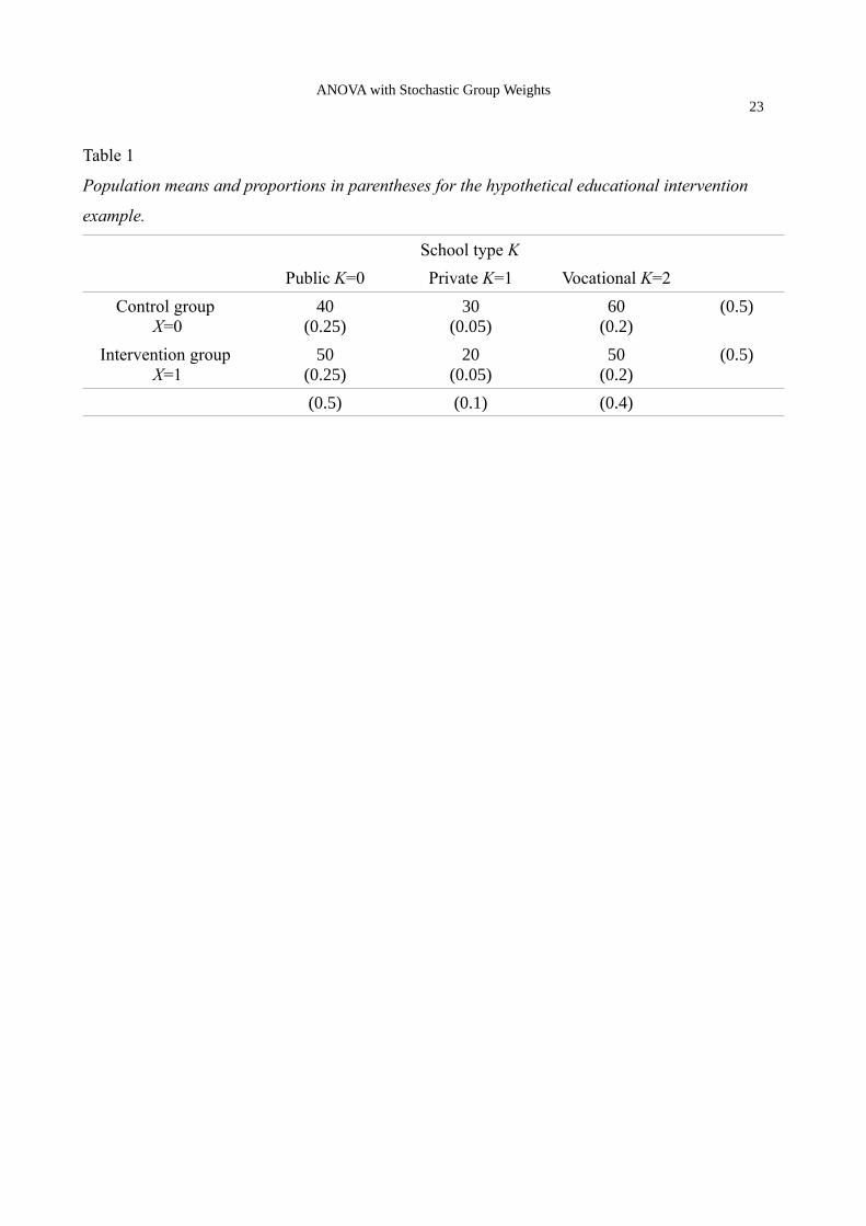
design. Assume we know the population means and marginal probabilities which are depicted in
Table 1.
Table 1 to appear about here
Comparing the population means between the intervention group and the control group, we see that
the mathematics training has a positive effect +10 in public schools and a negative effect -10 in
1 In some statistical software packages it is not easy to get such average effects (like in SPSS) but in others there exist convenient functions (e.g. R packages lsmeans or emmeans). To the best of our knowledge, EffectLiteR (Mayer & Dietzfelbinger, 2018) is the only software package that now allows for incorporating stochastic group weights.
2 Notice that our distinction between fixed and stochastic group weights is not related to treating factors as fixed or random, which is sometimes emphasized in the ANOVA literature. In this literature fixed factors are categorical variables with a fixed number of levels that are all observed in each sample, and random factors are categorical variables, such as the person variable or a school-ID, that have a large number of levels and the realized levels in the sample are a random sample of all possible levels and can therefore be different in each sample. In this sense, we consider fixed factors with stochastic group sizes in this paper.
ANOVA with Stochastic Group Weights5
private and vocational schools. The average effect is zero, because 50% of the population attend
public schools and 50% attend private or vocational schools, so each of the two effects gets a
weight of 0.5. Notice that this is a randomized experiment, and therefore X (intervention status) and
K (school type) are independent, i.e., the cell probabilities are obtained as the product of the
marginal probabilities.
Now consider two different researchers who both collect data with sample size N=200 and
conduct an ANOVA to obtain tests for main effects, interactions, and contrasts based on marginal
means. The first researcher is using a design with stochastic group weights and the second
researcher is using a design with fixed group weights. Researcher 1 recruits a random sample of 200
adolescents, asks them which type of school they attend, and assigns each of them randomly to
either the intervention group or the control group with probability 0.5, e.g., by flipping a coin for
each participant. Of course, the cell probabilities in the sample are most likely not exactly equal to
the population probabilities but they would typically be close. If researcher 1 would repeat the
experiment, we would see some variability in cell probabilities in the samples but no systematic
deviations from the population values. In the fully stochastic design used by researcher 1 both X and
K are stochastic, i.e., the cell frequencies, the marginal frequencies of X and the marginal
frequencies of K vary (slightly) from sample to sample. Researcher 2 happens to know the
population probabilities and ensures that these are exactly the same in the sample by first recruiting
individuals from each school type based on the known proportions and then randomly assigning
exactly half of the individuals from each school type to the control and treatment condition, e.g., by
drawing assignments out of an urn with the same number of intervention and control group
assignments. So in this sample, there are 100 adolescents from public schools (50 in the control
group and 50 in the training group), 20 adolescents from private schools (10 in the control group
and 10 in the training group), and 80 adolescents from vocational schools (40 in the control group
and 40 in the training group). If researcher 2 would repeat the experiment, we would get identical
group sizes and cell probabilities in all samples. In this fully fixed design, the group weights are
fixed and therefore also the marginal frequencies of both X and K are fixed as well.
Notice that both researchers conduct a randomized experiment and data come from the same
population. Both researchers have the same research question and they use the same statistical
method. We argue that the design with stochastic group sizes used by researcher 1 is far more
common in social research research, because the true population probabilities are rarely known and
oftentimes not all predictors are under full control of the experimenter. Nevertheless, the ANOVA
method that assumes fixed group weights is frequently used to estimate effects in designs with
stochastic group weights.
ANOVA with Stochastic Group Weights6
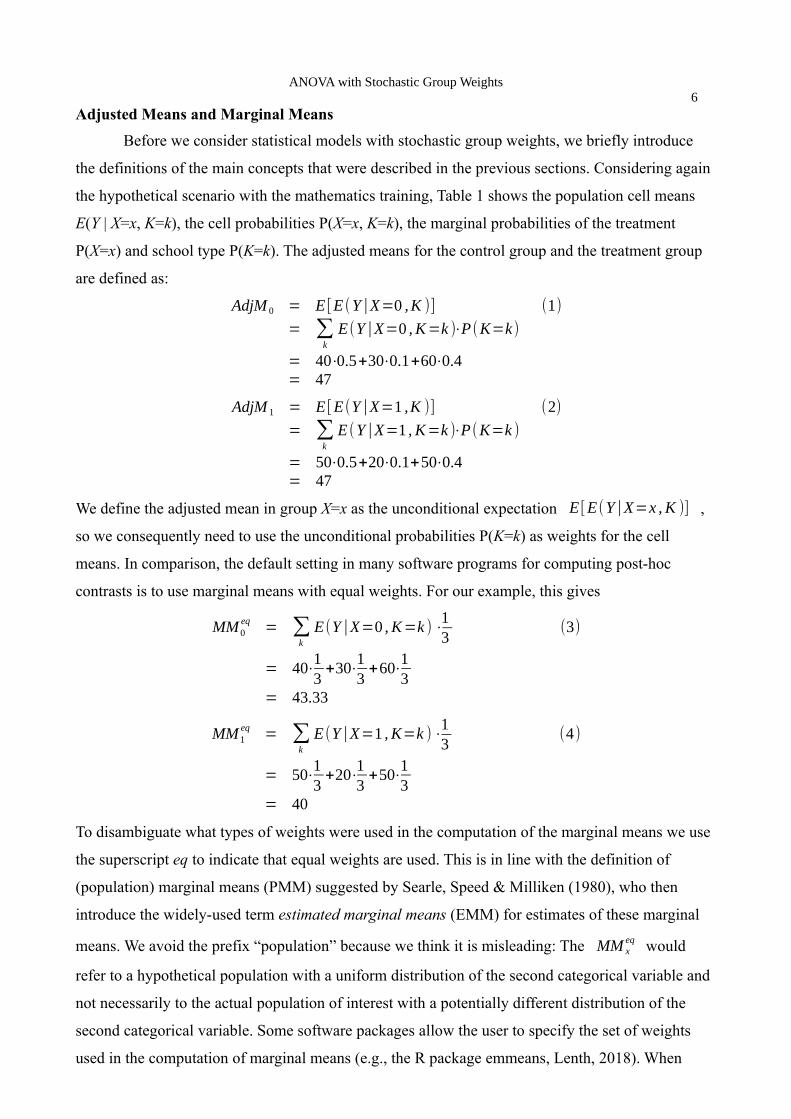
Adjusted Means and Marginal Means
Before we consider statistical models with stochastic group weights, we briefly introduce
the definitions of the main concepts that were described in the previous sections. Considering again
the hypothetical scenario with the mathematics training, Table 1 shows the population cell means
E(Y | X=x, K=k), the cell probabilities P(X=x, K=k), the marginal probabilities of the treatment
P(X=x) and school type P(K=k). The adjusted means for the control group and the treatment group
are defined as:
AdjM 0 = E [E (Y|X=0 ,K )] (1)= ∑
k
E(Y|X=0 , K=k )⋅P(K=k)
= 40⋅0.5+30⋅0.1+60⋅0.4= 47
AdjM 1 = E [E(Y|X=1 ,K )] (2)= ∑
k
E (Y|X=1 , K=k )⋅P(K=k )
= 50⋅0.5+20⋅0.1+50⋅0.4= 47
We define the adjusted mean in group X=x as the unconditional expectation E [E(Y|X=x , K )] ,
so we consequently need to use the unconditional probabilities P(K=k) as weights for the cell
means. In comparison, the default setting in many software programs for computing post-hoc
contrasts is to use marginal means with equal weights. For our example, this gives
MM0eq = ∑
k
E(Y|X=0 , K=k ) ⋅13
(3)
= 40⋅13
+30⋅13
+60⋅13
= 43.33
MM1eq = ∑
k
E(Y|X=1 , K=k )⋅13
(4)
= 50⋅13
+20⋅13
+50⋅13
= 40
To disambiguate what types of weights were used in the computation of the marginal means we use
the superscript eq to indicate that equal weights are used. This is in line with the definition of
(population) marginal means (PMM) suggested by Searle, Speed & Milliken (1980), who then
introduce the widely-used term estimated marginal means (EMM) for estimates of these marginal
means. We avoid the prefix “population” because we think it is misleading: The MM xeq would
refer to a hypothetical population with a uniform distribution of the second categorical variable and
not necessarily to the actual population of interest with a potentially different distribution of the
second categorical variable. Some software packages allow the user to specify the set of weights
used in the computation of marginal means (e.g., the R package emmeans, Lenth, 2018). When
ANOVA with Stochastic Group Weights7
proportional weights are specified, the marginal means MM xpro are identical to the adjusted means
as defined above and we can use standard software to obtain estimates for the adjusted means as we
show in Appendix A.
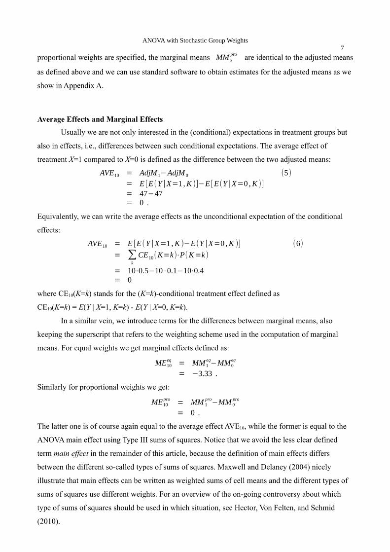
Average Effects and Marginal Effects
Usually we are not only interested in the (conditional) expectations in treatment groups but
also in effects, i.e., differences between such conditional expectations. The average effect of
treatment X=1 compared to X=0 is defined as the difference between the two adjusted means:
AVE10 = AdjM 1−AdjM 0 (5)= E [E(Y|X=1 , K )]−E [E(Y|X=0 , K )]= 47−47= 0 .
Equivalently, we can write the average effects as the unconditional expectation of the conditional
effects:
AVE10 = E [E(Y|X=1 , K )−E(Y|X=0 , K )] (6)= ∑
k
CE10(K=k)⋅P(K=k)
= 10⋅0.5−10⋅0.1−10⋅0.4= 0
where CE10(K=k) stands for the (K=k)-conditional treatment effect defined as
CE10(K=k) = E(Y | X=1, K=k) - E(Y | X=0, K=k).
In a similar vein, we introduce terms for the differences between marginal means, also
keeping the superscript that refers to the weighting scheme used in the computation of marginal
means. For equal weights we get marginal effects defined as:
ME10eq = MM1
eq−MM0eq
= −3.33 .
Similarly for proportional weights we get:
ME10pro = MM 1
pro−MM 0pro
= 0 .
The latter one is of course again equal to the average effect AVE10, while the former is equal to the
ANOVA main effect using Type III sums of squares. Notice that we avoid the less clear defined
term main effect in the remainder of this article, because the definition of main effects differs
between the different so-called types of sums of squares. Maxwell and Delaney (2004) nicely
illustrate that main effects can be written as weighted sums of cell means and the different types of
sums of squares use different weights. For an overview of the on-going controversy about which
type of sums of squares should be used in which situation, see Hector, Von Felten, and Schmid
(2010).
ANOVA with Stochastic Group Weights8
Models with Stochastic Group Weights
Having introduced the most important concept at the population level, we now turn to
presenting two different statistical models with stochastic group weights that both can be used to
estimate adjusted means as well as average effects based on a sample. They can also be used to
obtain overall hypothesis tests as is common for ANOVA-like methods. The first model is based on
the general linear model where the group weights are added to the model. The second model is a
special case of the general EffectLiteR model (Mayer et al., 2016) and uses maximum likelihood
estimation for a multigroup structural equation model with stochastic group weights. Both models
along with the computation of all parameters and hypothesis tests of interest are implemented in the
R software package EffectLiteR (Mayer & Dietzfelbinger, 2018). The R code for analyzing the
teaching intervention example is provided in Appendix A.
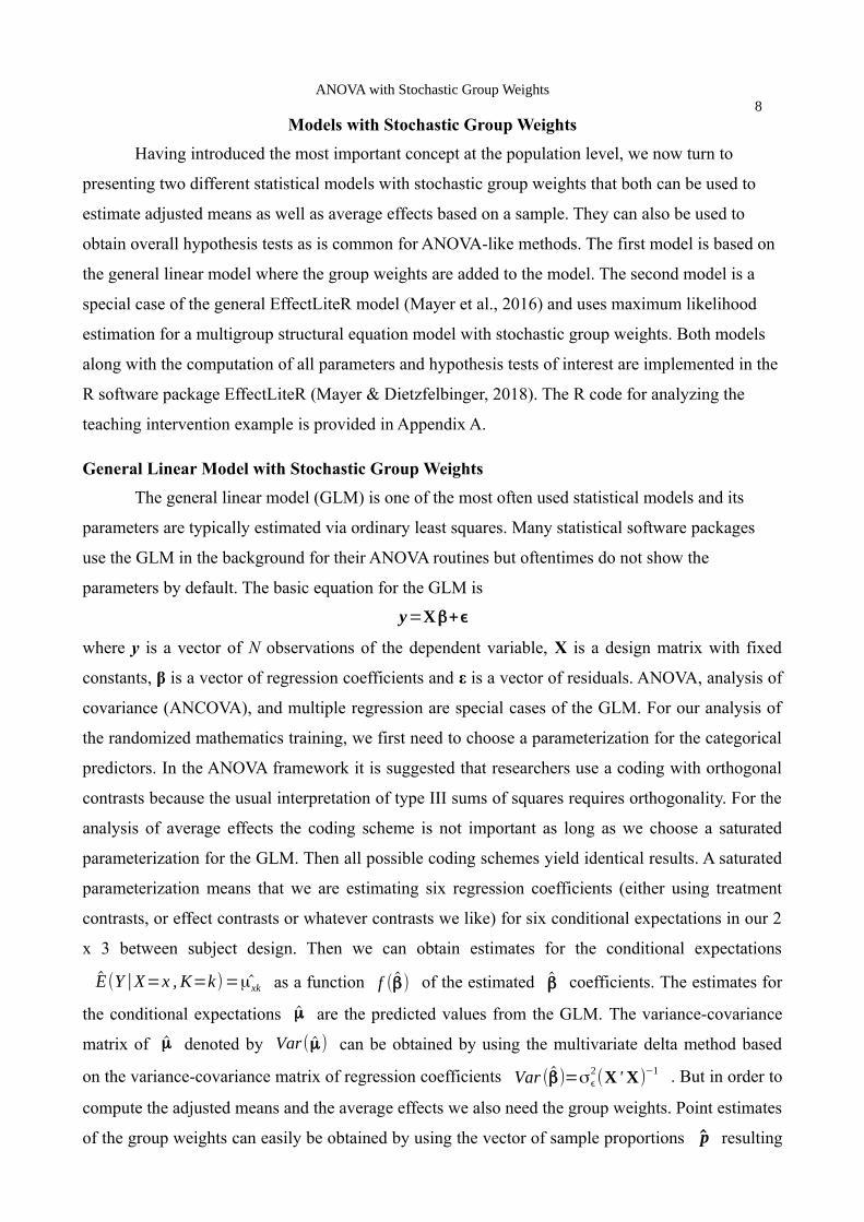
General Linear Model with Stochastic Group Weights
The general linear model (GLM) is one of the most often used statistical models and its
parameters are typically estimated via ordinary least squares. Many statistical software packages
use the GLM in the background for their ANOVA routines but oftentimes do not show the
parameters by default. The basic equation for the GLM is
y=Xβ+ϵ
where y is a vector of N observations of the dependent variable, X is a design matrix with fixed
constants, β is a vector of regression coefficients and ε is a vector of residuals. ANOVA, analysis of
covariance (ANCOVA), and multiple regression are special cases of the GLM. For our analysis of
the randomized mathematics training, we first need to choose a parameterization for the categorical
predictors. In the ANOVA framework it is suggested that researchers use a coding with orthogonal
contrasts because the usual interpretation of type III sums of squares requires orthogonality. For the
analysis of average effects the coding scheme is not important as long as we choose a saturated
parameterization for the GLM. Then all possible coding schemes yield identical results. A saturated
parameterization means that we are estimating six regression coefficients (either using treatment
contrasts, or effect contrasts or whatever contrasts we like) for six conditional expectations in our 2
x 3 between subject design. Then we can obtain estimates for the conditional expectations
E(Y|X=x , K=k)=μxk as a function f (β) of the estimated β coefficients. The estimates for
the conditional expectations μ are the predicted values from the GLM. The variance-covariance
matrix of μ denoted by Var(μ) can be obtained by using the multivariate delta method based
on the variance-covariance matrix of regression coefficients Var (β)=σϵ2(X 'X)−1 . But in order to
compute the adjusted means and the average effects we also need the group weights. Point estimates
of the group weights can easily be obtained by using the vector of sample proportions p resulting
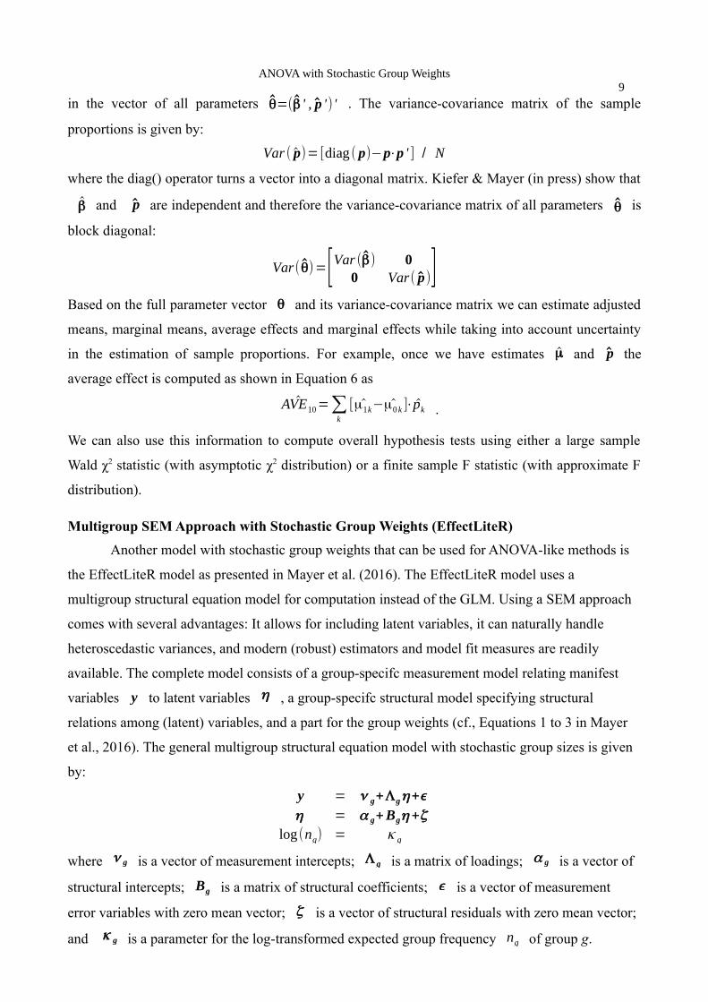
ANOVA with Stochastic Group Weights9
in the vector of all parameters θ=(β ' , p ') ' . The variance-covariance matrix of the sample
proportions is given by:
Var ( p)=[diag ( p)−p⋅p ' ] / N
where the diag() operator turns a vector into a diagonal matrix. Kiefer & Mayer (in press) show that
β and p are independent and therefore the variance-covariance matrix of all parameters θ is
block diagonal:
Var(θ)=[Var (β) 00 Var( p)]
Based on the full parameter vector θ and its variance-covariance matrix we can estimate adjusted
means, marginal means, average effects and marginal effects while taking into account uncertainty
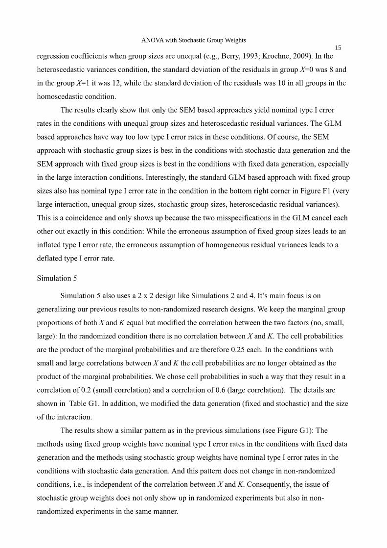
in the estimation of sample proportions. For example, once we have estimates μ and p the
average effect is computed as shown in Equation 6 as
^AVE10=∑k
[ ^μ1k− ^μ0 k ]⋅pk .
We can also use this information to compute overall hypothesis tests using either a large sample
Wald χ2 statistic (with asymptotic χ2 distribution) or a finite sample F statistic (with approximate F
distribution).
Multigroup SEM Approach with Stochastic Group Weights (EffectLiteR)
Another model with stochastic group weights that can be used for ANOVA-like methods is
the EffectLiteR model as presented in Mayer et al. (2016). The EffectLiteR model uses a
multigroup structural equation model for computation instead of the GLM. Using a SEM approach
comes with several advantages: It allows for including latent variables, it can naturally handle
heteroscedastic variances, and modern (robust) estimators and model fit measures are readily
available. The complete model consists of a group-specifc measurement model relating manifest
variables y to latent variables η , a group-specifc structural model specifying structural
relations among (latent) variables, and a part for the group weights (cf., Equations 1 to 3 in Mayer
et al., 2016). The general multigroup structural equation model with stochastic group sizes is given
by:
y = ν g+Λgη+ϵη = α g+Bgη+ζ
log(ng) = κ g
where ν g is a vector of measurement intercepts; Λ g is a matrix of loadings; α g is a vector of
structural intercepts; Bg is a matrix of structural coefficients; ϵ is a vector of measurement
error variables with zero mean vector; ζ is a vector of structural residuals with zero mean vector;
and κ g is a parameter for the log-transformed expected group frequency ng of group g.
ANOVA with Stochastic Group Weights10
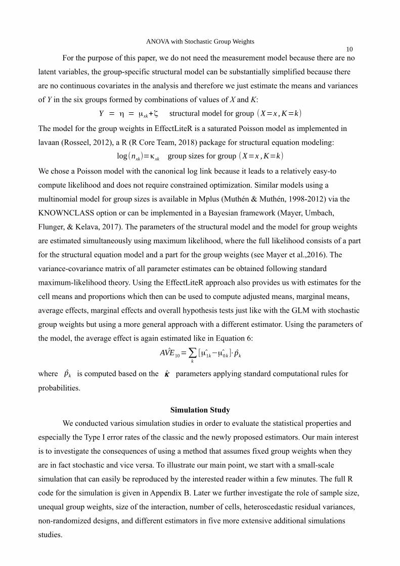
For the purpose of this paper, we do not need the measurement model because there are no
latent variables, the group-specific structural model can be substantially simplified because there
are no continuous covariates in the analysis and therefore we just estimate the means and variances
of Y in the six groups formed by combinations of values of X and K:
Y = η = μxk+ζ structural model for group (X=x , K=k)
The model for the group weights in EffectLiteR is a saturated Poisson model as implemented in
lavaan (Rosseel, 2012), a R (R Core Team, 2018) package for structural equation modeling:
log (nxk)=κxk group sizes for group (X=x , K=k)
We chose a Poisson model with the canonical log link because it leads to a relatively easy-to
compute likelihood and does not require constrained optimization. Similar models using a
multinomial model for group sizes is available in Mplus (Muthén & Muthén, 1998-2012) via the
KNOWNCLASS option or can be implemented in a Bayesian framework (Mayer, Umbach,
Flunger, & Kelava, 2017). The parameters of the structural model and the model for group weights
are estimated simultaneously using maximum likelihood, where the full likelihood consists of a part
for the structural equation model and a part for the group weights (see Mayer et al.,2016). The
variance-covariance matrix of all parameter estimates can be obtained following standard
maximum-likelihood theory. Using the EffectLiteR approach also provides us with estimates for the
cell means and proportions which then can be used to compute adjusted means, marginal means,
average effects, marginal effects and overall hypothesis tests just like with the GLM with stochastic
group weights but using a more general approach with a different estimator. Using the parameters of
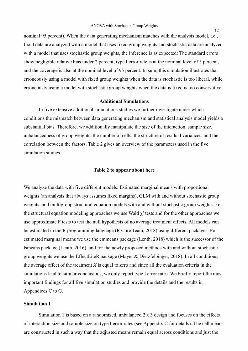
the model, the average effect is again estimated like in Equation 6:
^AVE10=∑k
[ ^μ1k− ^μ0 k ]⋅pk
where pk is computed based on the κ parameters applying standard computational rules for
probabilities.
Simulation Study
We conducted various simulation studies in order to evaluate the statistical properties and
especially the Type I error rates of the classic and the newly proposed estimators. Our main interest
is to investigate the consequences of using a method that assumes fixed group weights when they
are in fact stochastic and vice versa. To illustrate our main point, we start with a small-scale
simulation that can easily be reproduced by the interested reader within a few minutes. The full R
code for the simulation is given in Appendix B. Later we further investigate the role of sample size,
unequal group weights, size of the interaction, number of cells, heteroscedastic residual variances,
non-randomized designs, and different estimators in five more extensive additional simulations
studies.
ANOVA with Stochastic Group Weights11
Design
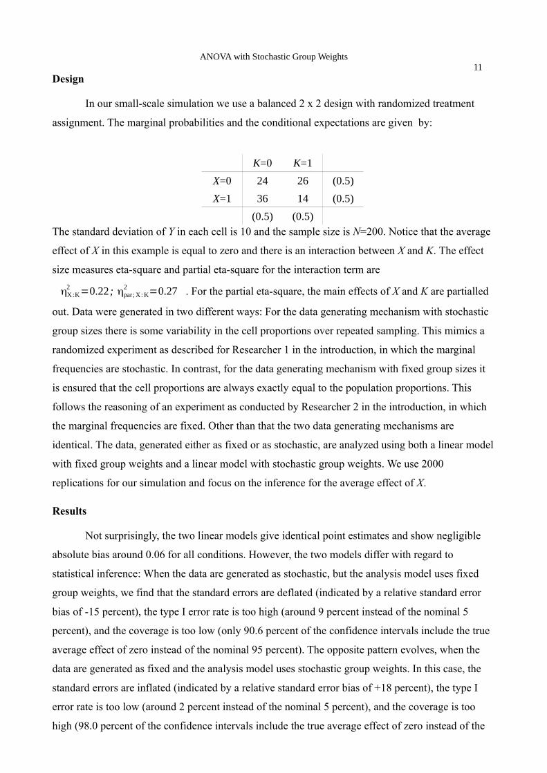
In our small-scale simulation we use a balanced 2 x 2 design with randomized treatment
assignment. The marginal probabilities and the conditional expectations are given by:
K=0 K=1
X=0 24 26 (0.5)
X=1 36 14 (0.5)
(0.5) (0.5)The standard deviation of Y in each cell is 10 and the sample size is N=200. Notice that the average
effect of X in this example is equal to zero and there is an interaction between X and K. The effect
size measures eta-square and partial eta-square for the interaction term are
ηX:K2 =0.22; ηpar ; X: K
2 =0.27 . For the partial eta-square, the main effects of X and K are partialled
out. Data were generated in two different ways: For the data generating mechanism with stochastic
group sizes there is some variability in the cell proportions over repeated sampling. This mimics a
randomized experiment as described for Researcher 1 in the introduction, in which the marginal
frequencies are stochastic. In contrast, for the data generating mechanism with fixed group sizes it
is ensured that the cell proportions are always exactly equal to the population proportions. This
follows the reasoning of an experiment as conducted by Researcher 2 in the introduction, in which
the marginal frequencies are fixed. Other than that the two data generating mechanisms are
identical. The data, generated either as fixed or as stochastic, are analyzed using both a linear model
with fixed group weights and a linear model with stochastic group weights. We use 2000
replications for our simulation and focus on the inference for the average effect of X.
Results
Not surprisingly, the two linear models give identical point estimates and show negligible
absolute bias around 0.06 for all conditions. However, the two models differ with regard to
statistical inference: When the data are generated as stochastic, but the analysis model uses fixed
group weights, we find that the standard errors are deflated (indicated by a relative standard error
bias of -15 percent), the type I error rate is too high (around 9 percent instead of the nominal 5
percent), and the coverage is too low (only 90.6 percent of the confidence intervals include the true
average effect of zero instead of the nominal 95 percent). The opposite pattern evolves, when the
data are generated as fixed and the analysis model uses stochastic group weights. In this case, the
standard errors are inflated (indicated by a relative standard error bias of +18 percent), the type I
error rate is too low (around 2 percent instead of the nominal 5 percent), and the coverage is too
high (98.0 percent of the confidence intervals include the true average effect of zero instead of the
ANOVA with Stochastic Group Weights12
nominal 95 percent). When the data generating mechanism matches with the analysis model, i.e.,
fixed data are analyzed with a model that uses fixed group weights and stochastic data are analyzed
with a model that uses stochastic group weights, the inference is as expected: The standard errors
show negligible relative bias under 2 percent, type I error rate is at the nominal level of 5 percent,
and the coverage is also at the nominal level of 95 percent. In sum, this simulation illustrates that
erroneously using a model with fixed group weights when the data is stochastic is too liberal, while
erroneously using a model with stochastic group weights when the data is fixed is too conservative.
Additional Simulations
In five extensive additional simulations studies we further investigate under which
conditions the mismatch between data generating mechanism and statistical analysis model yields a
substantial bias. Therefore, we additionally manipulate the size of the interaction, sample size,
unbalancedness of group weights, the number of cells, the structure of residual variances, and the
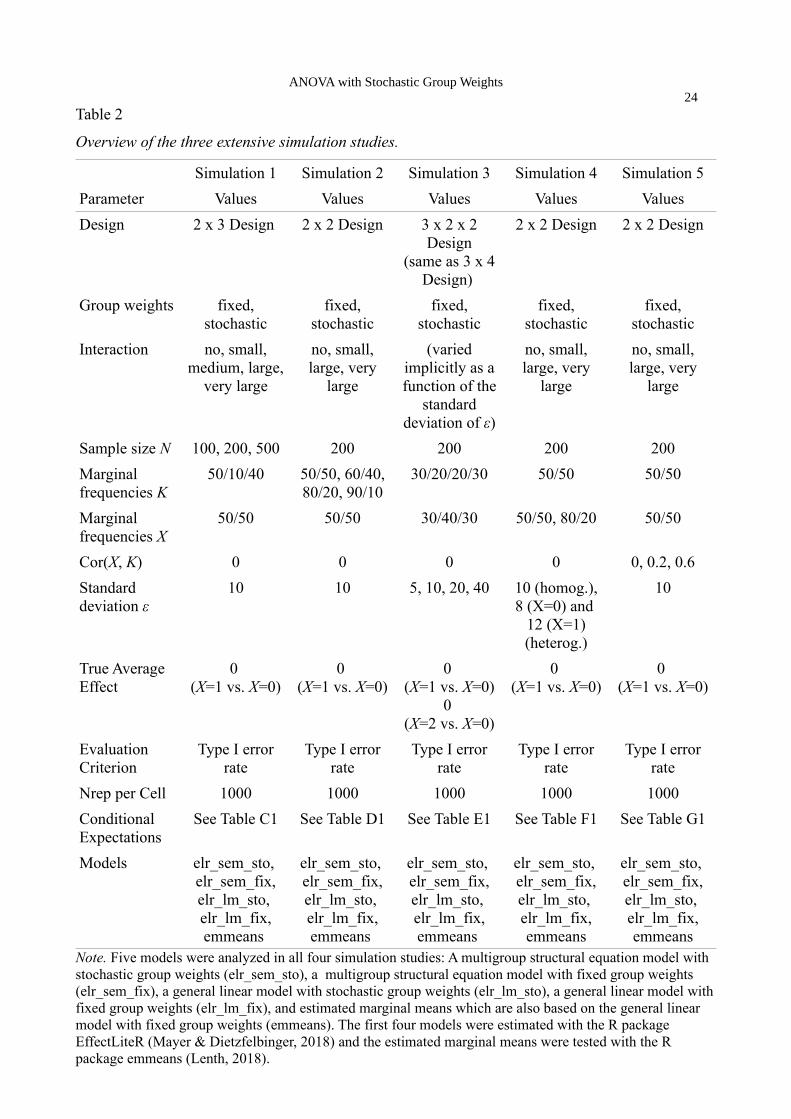
correlation between the factors. Table 2 gives an overview of the parameters used in the five
simulation studies.
Table 2 to appear about here
We analyze the data with five different models: Estimated marginal means with proportional
weights (an analysis that always assumes fixed margins), GLM with and without stochastic group
weights, and multigroup structural equation models with and without stochastic group weights. For
the structural equation modeling approaches we use Wald χ2 tests and for the other approaches we
use approximate F tests to test the null hypothesis of no average treatment effects. All models can
be estimated in the R programming language (R Core Team, 2018) using different packages: For
estimated marginal means we use the emmeans package (Lenth, 2018) which is the successor of the
lsmeans package (Lenth, 2016), and for the newly proposed methods with and without stochastic
group weights we use the EffectLiteR package (Mayer & Dietzfelbinger, 2018). In all conditions,
the average effect of the treatment X is equal to zero and since all the evaluation criteria in the
simulations lead to similar conclusions, we only report type I error rates. We briefly report the most
important findings for all five simulation studies and provide the details and the results in
Appendices C to G.
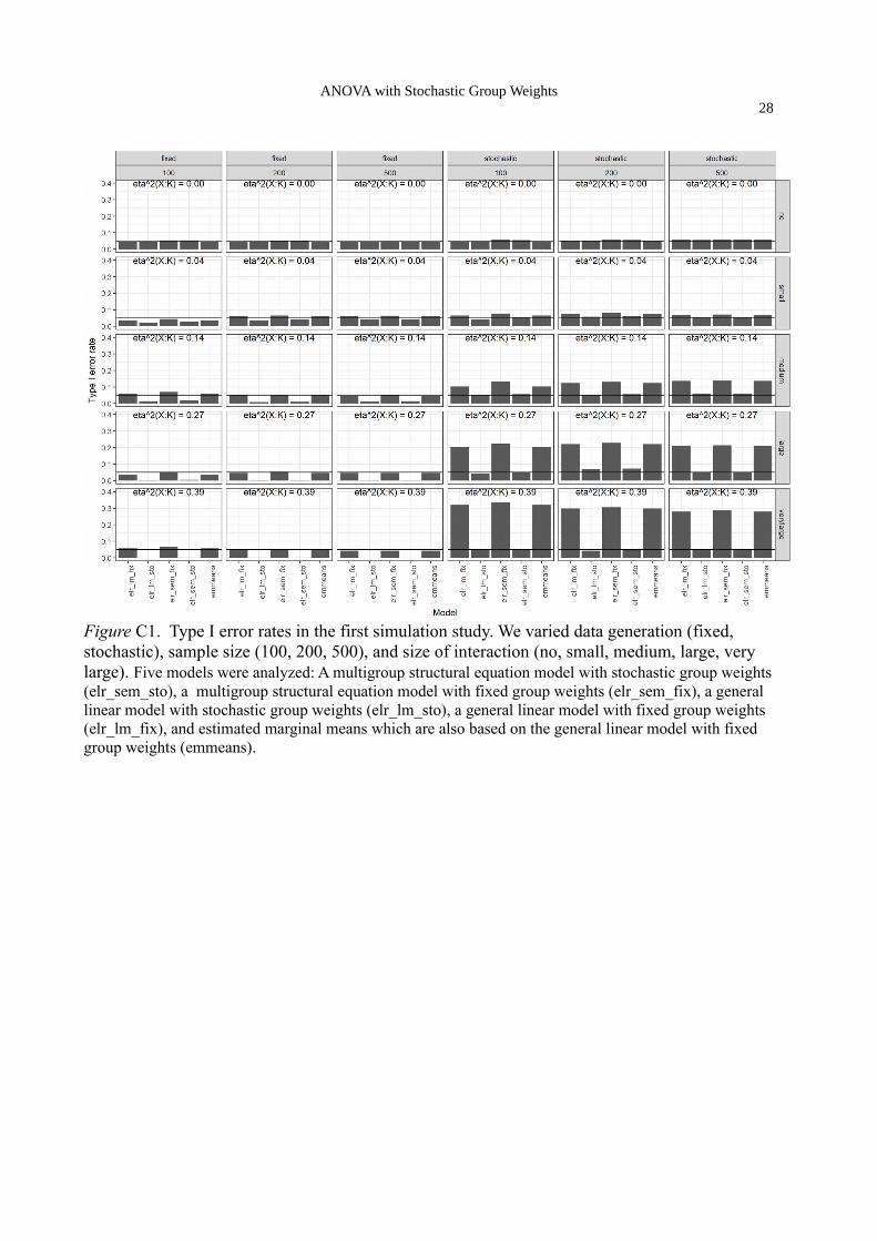
Simulation 1
Simulation 1 is based on a randomized, unbalanced 2 x 3 design and focuses on the effects
of interaction size and sample size on type I error rates (see Appendix C for details). The cell means
are constructed in such a way that the adjusted means remain equal across conditions and just the

ANOVA with Stochastic Group Weights13
size of the interaction is varied. As in our our small-scale simulation we find that the models that
erroneously assume fixed group weights have an inflated type I error rate. This finding crucially
depends on the size of the interaction: For medium interactions (ηX: K2 =0.14 ; ηpar ; X: K
2 =0.39) , the
type I error rate is around 10 percent, for large interactions (ηX: K2 =0.27 ; ηpar ; X: K
2 =0.59) , the type
I error rate is around 20 percent, and for very large interactions (ηX: K2 =0.39; ηpar ;X :K
2 =0.72) , the
type I error rate is around 30 percent. The inflation of type I error rates is negligible in conditions
with no or small interactions. Correctly specified models have nominal type I error rates in all
conditions. Interestingly, these findings are totally independent of sample size. We also do not find
differences between using Wald χ2 tests as for the SEM based models or F tests as for the GLM
based models.
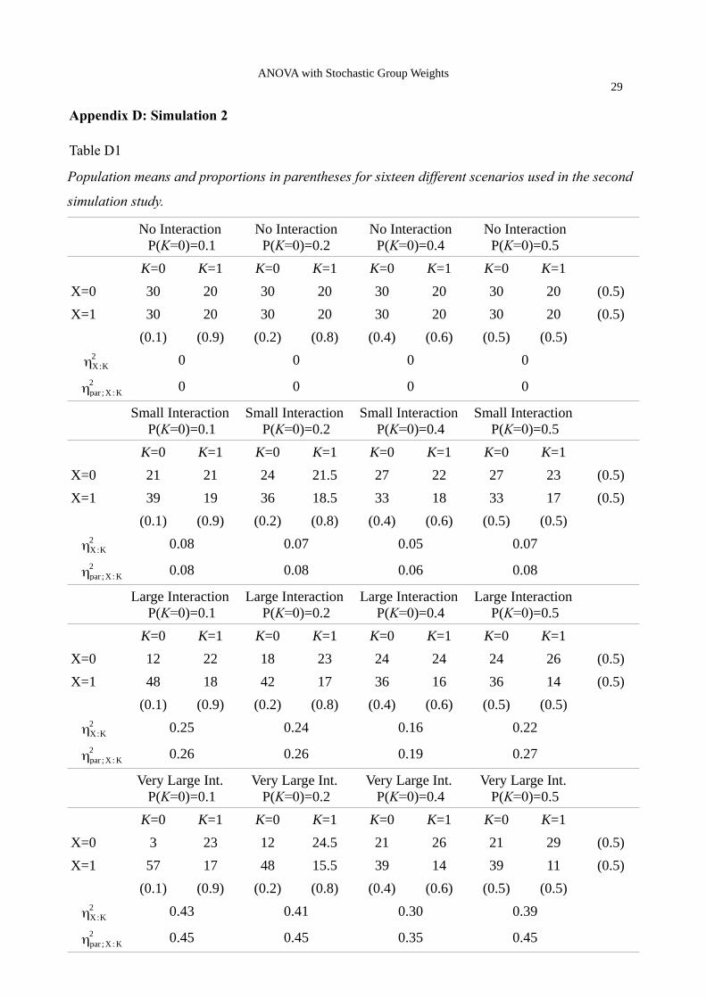
Simulation 2
Simulation 2 is based on a randomized 2 x 2 design and focuses on the effects of
unbalancedness on type I error rates (see Appendix D for details). Unbalancedness is manipulated
by using different marginal group proportions for K ranging from balanced (50/50) to highly
unbalanced (10/90). Since the interaction size turned out to be a crucial parameter, we also
manipulated the size of the interaction in simulation 2. The cell means are again constructed in such
a way that the adjusted means remain equal across conditions and that the average effect of X is
zero in all conditions. The key findings are the same as in our previous simulations and are not
repeated here. Interestingly, the amount of unbalancedness is irrelevant for the inflation of type I
error rates. The only significant factor is again the size of the interaction.
When comparing the results from Simulations 1 and 2 we find that the inflation of type I
error rates are considerably higher in Simulation 1. For example, in the very large interaction
condition, the type I error rate in Simulation 1 is around 30 percent, whereas it is around 13 percent
in Simulation 2. There are two key differences between the simulation studies that could cause this
discrepancy: First, it could be due to the number of values of K. Since we need to average over K,
more group weights enter the computation of the average effect in Simulation 1. Second, the
average effect of K is higher in Simulation 1, leading to a higher amount of overall variance
explained (R2) and therefore to much greater effect sizes of the interaction in terms of partial η2. To
figure out which causes the discrepancy in type I error rates between Simulation 1 and 2, we
conducted a third simulation study with more levels of K, in which we also manipulated the average
effect of K.

ANOVA with Stochastic Group Weights14
Simulation 3
Simulation 3 is based on a randomized 3 x 2 x 2 design and focuses on the consequences of
the average effect of K on type I error rates for the average effect of X (see Appendix E for details).
Notice that the overall amount of variance explained in the outcome (R2) changes as well by
manipulating the average effect of K. In contrast to previous simulations, X can take on three values
and the reported tests for average effects are joined tests that there is no average effect of X=1 vs.
X=0 and there is no average effect of X=2 vs. X=0. Since we focus on the effects of X, we need to
average over the 2 x 2 combinations of values of the other two categorical variables K1 and K2. This
is computationally equivalent to a 3 x 4 design with a K variable that can take on four values. The
data are generated in such a way that the absolute size of the interaction and the conditional effects
of X remain the same across a low R2 and high R2 condition. In the low R2 condition there is no
average effect of K while there is a strong average effect of K in the high R2 condition. Because the
absolute size of the interaction and the residual error variance remain the same, the partial η2 for the
interaction term is the same in both low and high R2 conditions, but the η2 for the interaction term
can be quite different between low and high R2 conditions. The size of the interaction is
manipulated indirectly by using different values for the residual standard deviation SD(ε).
The results clearly illustrate that the key factor for the inflation of type I error rates is the
partial η2. Within the large interaction condition, the type I error rate is almost identical for the low
and high R2 conditions, even though the η2 is much lower for the high R2 condition. However, the
partial η2 is identical for both conditions which explains that they have almost identical type I error
rates. The number of levels of K is not important as can be seen by comparing results across the
simulations: In conditions with similar partial η2 values we always find comparable type I error
rates, no matter if we average over two (as in Simulation 2), three (as in Simulation 1) or four (as in
Simulation 3) values of K.
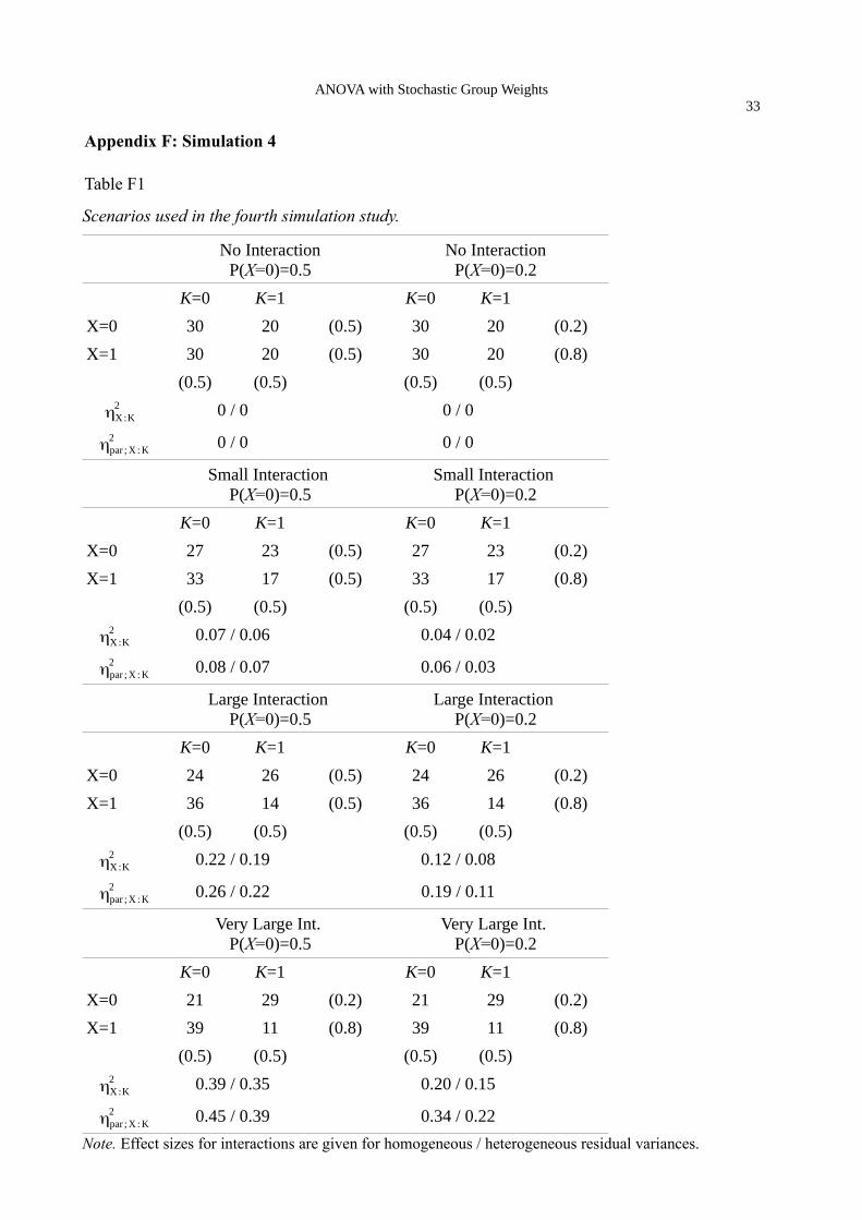
Simulation 4
Simulation 4 uses a 2 x 2 design like Simulation 2. It’s main focus is on comparing our first
proposed approach based on the general linear model to our second approach based on the
multigroup SEM (see Appendix F for details). The SEM based approach uses a multigroup model
and can easily incorporate unequal residual variances across groups. Therefore we expect to see an
advantage of the SEM approach in conditions with heteroscedastic residual variances. The
considered scenarios are similar to those in Simulation 2, but instead of manipulating the marginal
group proportions of K, which did not make a difference, we manipulated the marginal group
proportions of X (with two conditions, 50/50 and 20/80), because it is well-known in the literature
that violation of homoscedasticity is critical with respect to the standard error of estimated
ANOVA with Stochastic Group Weights15
regression coefficients when group sizes are unequal (e.g., Berry, 1993; Kroehne, 2009). In the
heteroscedastic variances condition, the standard deviation of the residuals in group X=0 was 8 and
in the group X=1 it was 12, while the standard deviation of the residuals was 10 in all groups in the
homoscedastic condition.
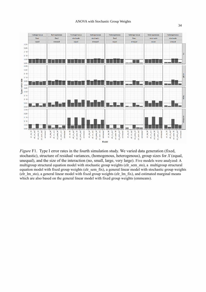
The results clearly show that only the SEM based approaches yield nominal type I error
rates in the conditions with unequal group sizes and heteroscedastic residual variances. The GLM
based approaches have way too low type I error rates in these conditions. Of course, the SEM
approach with stochastic group sizes is best in the conditions with stochastic data generation and the
SEM approach with fixed group sizes is best in the conditions with fixed data generation, especially
in the large interaction conditions. Interestingly, the standard GLM based approach with fixed group
sizes also has nominal type I error rate in the condition in the bottom right corner in Figure F1 (very
large interaction, unequal group sizes, stochastic group sizes, heteroscedastic residual variances).
This is a coincidence and only shows up because the two misspecifications in the GLM cancel each
other out exactly in this condition: While the erroneous assumption of fixed group sizes leads to an
inflated type I error rate, the erroneous assumption of homogeneous residual variances leads to a
deflated type I error rate.
Simulation 5
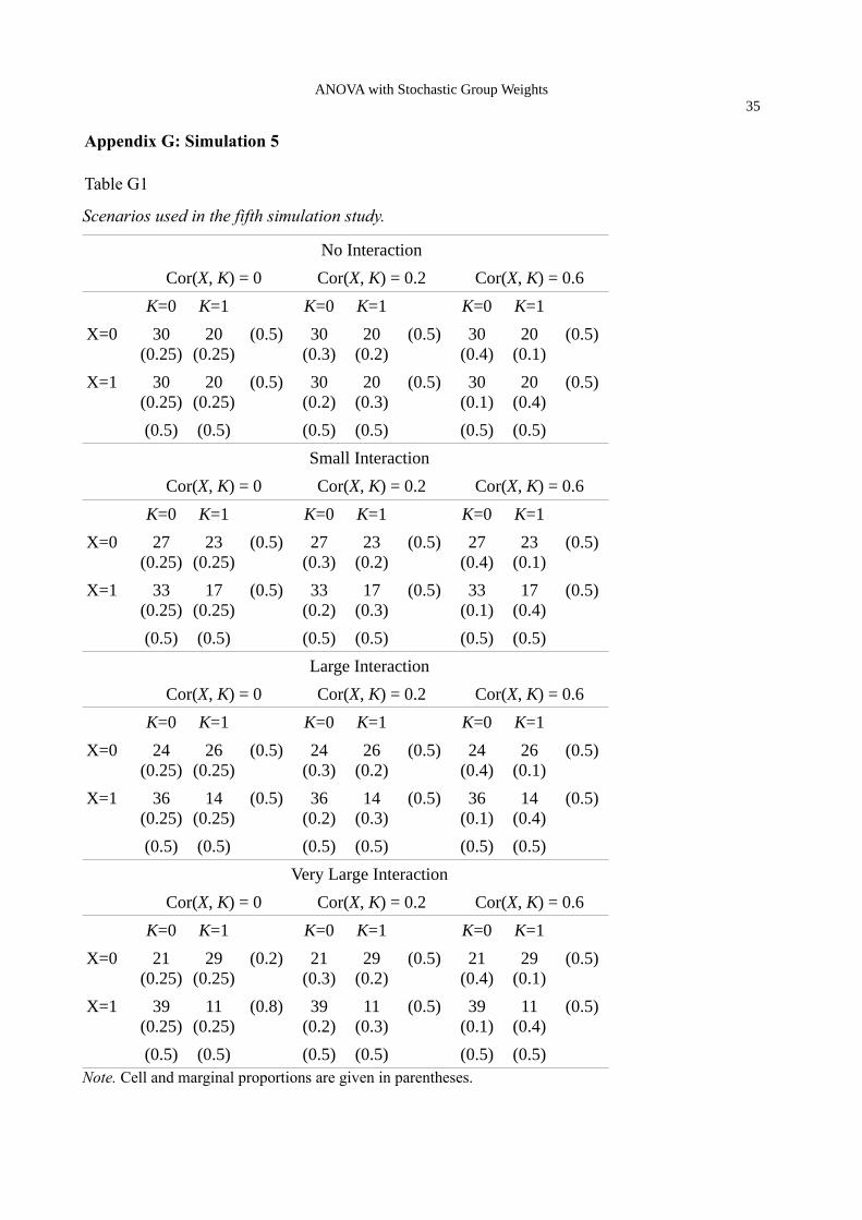
Simulation 5 also uses a 2 x 2 design like Simulations 2 and 4. It’s main focus is on
generalizing our previous results to non-randomized research designs. We keep the marginal group
proportions of both X and K equal but modified the correlation between the two factors (no, small,
large): In the randomized condition there is no correlation between X and K. The cell probabilities
are the product of the marginal probabilities and are therefore 0.25 each. In the conditions with
small and large correlations between X and K the cell probabilities are no longer obtained as the
product of the marginal probabilities. We chose cell probabilities in such a way that they result in a
correlation of 0.2 (small correlation) and a correlation of 0.6 (large correlation). The details are
shown in Table G1. In addition, we modified the data generation (fixed and stochastic) and the size
of the interaction.
The results show a similar pattern as in the previous simulations (see Figure G1): The
methods using fixed group weights have nominal type I error rates in the conditions with fixed data
generation and the methods using stochastic group weights have nominal type I error rates in the
conditions with stochastic data generation. And this pattern does not change in non-randomized
conditions, i.e., is independent of the correlation between X and K. Consequently, the issue of
stochastic group weights does not only show up in randomized experiments but also in non-
randomized experiments in the same manner.

ANOVA with Stochastic Group Weights16
Discussion
In this paper we discussed the issue of stochastic group sizes in factorial ANOVA designs.
Even though stochastic group sizes are probably the norm, rather than the exception, in social
science research, they are typically ignored in the data analysis. In fact, Keselman et al. (1998)
show in their review that 72 percent of the between-subject factorial designs in educational research
are unbalanced. Yet, the standard ANOVA approach is used almost exclusively, and we argue that
there is essentially no awareness of this issue in the psychological community. This approach, as we
have explained, does not by default integrate the uncertainty that arises from stochastic cell sizes.
Using a simple simulation study, we have shown that ignoring the uncertainty in the
sampling process, leads to a negative bias in standard errors, and resulting from this to Type I error
inflation, and coverage intervals that are lower than their nominal level. In further simulation
studies, we were able to demonstrate that the magnitude of the interaction is a critical component as
to how much bias is introduced. Generally speaking, the larger the interaction in the factorial
design, the more bias will be introduced when the stochastic nature of the sampling procedure is
ignored. An interesting aspect of these simulations studies is that this type of bias also happens in
randomized studies, and is not much influenced by sample size, or the particular design (e.g.,
number of groups, or imbalance of the design).
We have proposed two new ways that allow to incorporate stochastic sampling plans, either
using GLM methods that include the information on stochastic group sizes, or using a maximum
likelihood-based multigroup SEM approach. Both of these approaches account for the uncertainty
in the sampling process, and yield unbiased estimates of the standard errors, and therefore nominal
Type I error and coverage rates. The SEM based approach can additionally deal with
heteroscedastic residual variances and latent variables. Our recommendation therefore follows
naturally, that we urge researchers who use stochastic group sizes, to rely on methods that estimate
the uncertainty that comes with these methods, and provide trustworthy inferential statistics.
Generalizations
Non-randomized experiments: In this paper we focused on randomized experiments and
briefly showed in Simulation 5 that the issue of stochastic group weights generalizes to non-
randomized experiments. Stochastic group weights can be present in all types of studies in which
researchers want to estimate average or conditional effects, while taking into account interactions
between a cause and categorical covariates. The proposed procedure of estimating the stochastic
group weights and incorporating them in the computation of average effects is directly applicable in
non-randomized settings as well. However, in non-randomized experiments there can be a
stochastic dependency between the treatment variable and the other categorical (and continuous)
ANOVA with Stochastic Group Weights17
variables. Therefore, considering additional categorical and continuous variables in the analysis is
essential not only for gaining efficiency but also to obtain unbiased estimates for the average effects
in such studies. In order for the average effects to have a causal interpretation in non-randomized
experiments, additional causality assumptions such as strong ignorability (Rosenbaum & Rubin,
1983) or another causality condition needs to be fulfilled (see also Imbens, 2004; Steyer, Gabler,
von Davier & Nachtigall, 2000).
Continuous covariates: We looked at experimental designs with categorical covariates only
and did not consider examples with continuous covariates. However, the proposed approach can be
generalized to such models including continuous covariates. A simple way to incorporate
continuous covariates in the analysis is to add grand-mean centered continuous covariates (Aiken &
West, 1996) as regressors either to the GLM based approach or to the SEM based approach and then
proceed as suggested in this paper. However, mean centering the continuous covariates again treats
the mean of the covariates as fixed and known and ignores uncertainty in the estimation of the
population mean. Just like ignoring uncertainty in the estimation of group weights, this may result
in an inflated type I error rate for the average effects (Kroehne, 2009; Liu, West, Levy, & Aiken,
2017; Sampson, 1974). Instead, estimates for the mean of the continuous variable can be added
along with a standard error and can then take into account for computing average effects. Mayer et
al. (2016) fully describe an example with a non-randomized 3 x 2 design and a continuous (latent)
covariate and also provide general formulas for computing average effects in such designs.
Comparisons to Other Methods
Post-stratification: A statistical technique that is closely related to the present paper is post-
stratification (Cochran, 1977; McHugh & Matts, 1983). In post-stratification the researcher stratifies
persons based on a pretreatment variable, estimates treatment effects within the strata and then uses
a weighted average of these strata estimates for the overall average treatment effect estimate
(Gelman & Little, 1997; Miratrix, Sekhon, & Yu, 2013). The definition of the average treatment
effect also originates from the causal inference literature and is identical with the definition we used
in the present paper. However, the rationale for deriving standard errors and confidence intervals for
the average effect is different: The post-stratification literature uses the Neyman-Rubin causal
model (Holland, 1986) to derive expressions for the standard errors of the sample average treatment
effect (SATE) and the population average treatment effect (PATE) based on potential outcomes
(Imbens & Rubin, 2015; Miratrix, Sekhon, & Yu, 2013; Neyman, 1923/1990). In contrast, we build
on the ANOVA and regression literature to derive standard errors for the average effect based on the
estimated regression coefficients and group sizes. Miratrix and colleagues claim that their “[...]
post-stratified estimator is identical to a fully saturated ordinary linear regression with the strata as
ANOVA with Stochastic Group Weights18
dummy variables and all strata-by-treatment interactions—i.e. a two-way analysis-of-variance
analysis with interactions.” (p. 382). So their post-stratified estimator for the SATE is identical to
our GLM based estimator with fixed group sizes and yields valid inferences when the group sizes
are fixed – or, equivalently, when only the sample average effect is of interest. In the settings we
considered the main interest is not in the SATE but in generalizing to a population, i.e., in
estimating the PATE. In this case we presume that our approaches with stochastic group sizes are
very similar (if not identical) to the post-stratified estimator for the PATE (Imbens, 2011; Miratrix et
al., 2013), even though the derivations and formulas are very different.
Weighted Effects Coding: In situations where the proportions of cases in each group in the
sample can be considered to represent the corresponding proportion of cases in the population,
Cohen, Cohen, Aiken and West (2003) recommend using weighted effects coding (see Chapter 8.4
on page 328ff). Weighted effects coding is straightforward to apply when there is only a single
factor. In this case, the regression coefficients represent the difference between the group means and
the weighted (overall) mean. However, weighted effects coding becomes much more complicated
when there are continuous or further categorical variables in the model, because interaction terms
cannot simply be created by multiplying the values of the two variables that make up the interaction
(Nieuwenhuis, te Grotenhuis, & Pelzer, 2017). Our approach differs from weighted effects coding
in multiple ways: First, we define our effects by comparing the groups with a reference group and
not with the weighted overall mean. Second, we provide clear definitions of average effects in the
presence of interactions based on conditional expectations and show how they can be computed.
Third, we take uncertainty in the estimation of group weights into account which is not done in
weighted effects coding.
Stochastic Regression: In stochastic regression the regressors are modeled as stochastic and
the joint distribution of the outcome and the regressors is considered (as opposed to the conditional
distribution of the outcome in ordinary least-squares regression). For regressions with identity link
function the estimation and inference for the regression coefficients is identical for both approaches
(see, e.g., Casella & Berger, 2002, p. 550). While there is no difference for the regression
coefficients, the key aspect of the present manuscript is the (subsequent) analysis of average or
main effects. And for this subsequent analysis it can make a difference whether we treat the
regressors (group weights) as fixed or as stochastic as we show in our simulations. So we need to
distinguish between treating the regressors as fixed/stochastic in the first step (i.e., when estimating
the regression coefficients; this is what stochastic regression is concerned about) and in the second
step (i.e., when estimating the average effects; this is the focus of the present paper).
ANOVA with Stochastic Group Weights19
Limitations
Our study tried to argue for the general point of being mindful of stochastic group sizes, but
there are some nuances that we did not explore in this paper. We only considered designs in which
all factors had fixed samples sizes, or in which all factors had stochastic sample sizes. Clearly, there
can be situations in which one factor has fixed sample sizes, and the other factor has stochastic
sample sizes, which we could refer to as mixed sample size design. For example, if researcher 2 in
our example in the paper would recruit individuals from each school type based on the exact known
proportions and would then randomly assign individuals using a coin toss to the control and
treatment condition, then X would be stochastic and K would be fixed. In such a mixed design, we
need to think about the nature of the variable that we average over for computing the average effect.
So when we compute the average effect of X we average over the distribution of fixed school type
K and therefore can use fixed group weights. When we compute the average effects of K (e.g., for
K=1 vs K=0 and K=2 vs. K=0), we average over the stochastic X and consequently need stochastic
group weights. We did not consider these designs directly, but based on our results, we strongly
conjecture that ignoring the stochastic nature of one factor, would yield similar issues to the one that
we described in the paper. For more complex experimental designs that eventually have structurally
empty cells or other distinct features, we also need to carefully think about the weighting scheme
we would like to use and whether the weights are stochastic or fixed.
In this paper, we neither fully discussed the causal interpretation and the causal definitions
for the effects, nor the causality conditions that are required for obtaining causal effects. However,
the definitions that we used for average effects and adjusted means originate from the causal
inference literature (e.g., Imbens & Rubin, 2015; Pearl, 2009; Rubin, 1974; Steyer, Mayer & Fiege,
2014). Given that there are no unobserved confounders, the average effect is the unconditional
expectation of the individual causal effects and the adjusted means are the expectations of the
individual potential or true outcomes in each treatment condition.
Our focus in the presentation of the our approaches was on studies in which the sample is a
random sample from the population. In survey research where more complicated sampling
procedures are used, the sampling design needs to be taken into account not only for the estimation
of regression coefficients but also for the estimation of the group weights. Otherwise we get biased
estimates for the group weights. Oftentimes the population proportions (from the Census or alike)
are used to determine the sampling scheme (e.g. oversampling of minorities) in a large scale survey.
In this case we recommend directly using the population proportions and treating them as fixed,
instead of using the biased estimates from the survey. An alternative is to correct the biased
estimates and recompute the population proportions taking into account the sampling scheme.
ANOVA with Stochastic Group Weights20
As we have illustrated throughout the paper, there are many situation where stochastic group
weights are more meaningful and we believe that they are an important addition to the statistical
toolbox of researchers. However, there are also situations where fixed group weights are more
appropriate. In balanced designs the group sizes have usually been fixed by the experimenter and
can therefore be considered fixed. Also in cases where the unbalancedness is not per se meaningful
but results from dropout or other difficulties in the data selection process, fixed group sizes can be
reasonable. In such cases, the researcher can also consider to use (fixed) equal group weights
instead of the observed unequal group weights. Another situation where fixed group weights are
adequate is when there is information on the true marginal probabilities of the categorical variables
that we average over. For instance, when we know, e.g., from Census data, the true proportions of
male and females in a population of interest, we can choose to use these true proportions in our
computations of adjusted means and average effects and consequently treat them as fixed. To
conclude, there are designs where fixed group weights are more appropriate and there are designs
where stochastic group weights are more appropriate and with this paper we give researchers the
opportunity to adequately address both types of designs in their analysis.
References
Aiken, L. S., & West, S. G. (1996). Multiple regression: Testing and interpreting interactions.
Thousand Oaks, CA: Sage.
Berry, W. D. (1993). Understanding regression assumptions. Thousand Oaks, CA: Sage
Publications.
Cochran, W. G. (1977). Sampling Techniques (3rd ed). New York: Wiley.
Cohen, J., Cohen, P., West, S. G., & Aiken, L. S. (2003). Applied multiple regression/correlation
analysis for the behavioral sciences. 3rd edition. Laurence Erlbaum Associates, Publishers,
Mahwah, NJ, USA.
Fisher, R. A. (1925). Statistical Methods for Research Workers, Oliver & Boyd, Edinburgh, London.
Fox, J., & Weisberg, S. (2011). An R Companion to Applied Regression (2nd ed.).
Thousand Oaks CA: Sage.
Gelman, A., & Little, T. C. (1997). Poststratification into many categories using hierarchical logistic
regression. Survey Methodology, 23, 127-135.
Goodnight, J. H., & Harvey, W. R. (1978). Least squares means in the fixed effects general linear
model. SAS Institute, Incorporated.
Hector, A., Von Felten, S., & Schmid, B. (2010). Analysis of variance with unbalanced data: An
update for ecology & evolution. Journal of Animal Ecology, 79, 308–316.

ANOVA with Stochastic Group Weights21
doi:10.1111/j.1365-2656.2009.01634.x
Holland, P. W. (1986) Statistics and causal inference. Journal of the American Statistical
Association, 81, 945–960.
Imbens, G. W. (2004). Nonparametric estimation of average treatment effects under exogeneity: A
review. Review of Economics and Statistics, 86, 4–29
Imbens, G. W. (2011) Experimental design for unit and cluster randomized trials. International
Initiative for Impact Evaluation, Cuernavaca.
Imbens, G. W., & Rubin, D. B. (2015). Causal inference in statistics, social, and biomedical
sciences. Cambridge University Press. doi: 10.1017/CBO9781139025751
Keselman, H. J., Huberty, C. J., Lix, L. M., Olejnik, S., Cribbie, R. A., Donahue, B., ..., Levin, J. R.
(1998). Statistical practices of educational researchers: An analysis of their ANOVA,
MANOVA, and ANCOVA analyses. Review of Educational Research, 68, 350–386. doi:
10.3102/00346543068003350
Keselman, H. J., Kowalchuk, R. K., & Lix, L. M. (1998). Robust nonorthogonal analyses
revisited: An update based on trimmed means. Psychometrika, 63, 145-163. doi:
10.1007/BF02294772
Kiefer, C., & Mayer, A. (in press). Average effects based on regressions with logarithmic link
function: A new approach with stochastic covariates. Psychometrika.
Kroehne, U. (2009). Estimation of average causal effects in quasi-experimental designs: Non-linear
constraints in structural equation models. (Unpublished doctoral dissertation). Friedrich-
Schiller-University, Jena, Germany.
Lenth, R. V. (2018). emmeans: Estimated marginal means, aka least-squares means. R package
version 1.1. https://CRAN.R-project.org/package=emmeans
Lenth, R. V. (2016). Least-squares means: The R package lsmeans. Journal of Statistical
Software, 69, 1-33. doi:10.18637/jss.v069.i01
Liu, Y., West, S. G., Levy, R., & Aiken, L. S. (2017). Tests of simple slopes in multiple regression
models with an interaction: Comparison of four approaches. Multivariate Behavioral
Research, 1–20.
Maxwell, S., & Delaney, H. (2004). Designing experiments and analyzing data: A model
comparison perspective. Mahwah, NJ: Lawrence Erlbaum
McHugh, R. and Matts, J. (1983). Post-stratification in the randomized clinical trial. Biometrics, 39,
217–225.
Mayer, A., & Dietzfelbinger, L. (2018). EffectLiteR: An R package for estimating average and
conditional effects. Retrieved from https://github.com/amayer2010/EffectLiteR.
Mayer, A., Dietzfelbinger, L., Rosseel, Y., & Steyer, R. (2016). The EffectLiteR approach for

ANOVA with Stochastic Group Weights22
analyzing average and conditional effects. Multivariate Behavioral Research, 51, 374-
391. doi: 10.1080/00273171.2016.1151334
Mayer, A., Flunger, B., Umbach, N., & Kelava, A. (2017). Effect analysis using nonlinear structural
equation mixture modeling. Structural Equation Modeling, 24, 556-570.
doi: 10.1080/10705511.2016.1273780
Miratrix, L. W., Sekhon, J. S., & Yu, B. (2013). Adjusting treatment effect estimates by post‐
stratification in randomized experiments. Journal of the Royal Statistical Society: Series B,
75, 369-396.
Muthén, L. K., & Muthén, B. O. (1998-2012). Mplus User’s Guide (7th ed.) [Computer software
manual]. Los Angeles, CA: Muthén & Muthén.
Nieuwenhuis, R., te Grotenhuis, H. F., & Pelzer, B. J. (2017). Weighted effect coding for
observational data with wec. The R Journal, 9, 477-485.
Pearl, J. (2009). Causality: Models, reasoning, and inference (2nd ed.). Cambridge, UK: Cambridge
University Press. doi: 10.1017/CBO9780511803161
R Core Team (2018). R: A language and environment for statistical computing. R Foundation for
Statistical Computing, Vienna, Austria. https://www.R-project.org/.
Rosenbaum, P. R. and Rubin, D. B. (1983). The central role of the propensity score in observational
studies for causal effects. Biometrika, 70, 41–55.
Rubin, D. B. (1974). Estimating causal effects of treatments in randomized and nonrandomized
studies. Journal of Educational Psychology, 66, 688–701. doi: 10.1037/h0037350
Sampson, A. R. (1974). A tale of two regressions. Journal of the American Statistical Association,
69, 682–689.
Searle, S. R., Speed, F. M., & Milliken, G. A. (1980). Population marginal means in the linear
model: an alternative to least squares means. The American Statistician, 34, 216-221.
Speed, F. M., Hocking, R. R., & Hackney, O. P. (1978). Methods of analysis of linear models with
unbalanced data. Journal of the American Statistical Association, 73, 105–112. doi:
10.1080/01621459.1978.10480012
Splawa-Neyman, J. (1923/1990). On the application of probability theory to agricultural
experiments: Essays on principles. Section 9. Statistical Science, 5, 465-480.
Steyer, R., Gabler, S., von Davier, A., & Nachtigall, C. (2000). Causal regression models II:
Unconfoundedness and causal unbiasedness. Methods of Psychological Research Online, 5,
55-86.
Steyer, R., Mayer, A., & Fiege, C. (2014). Causal inference on total, direct, and indirect effects. In
Michalos, A. C. (Ed.), Encyclopedia of Quality of Life and Well-Being Research (pp. 606–
631). Dordrecht, Netherlands: Springer. doi: 10.1007/978-94-007-0753-5_295
ANOVA with Stochastic Group Weights23
Table 1
Population means and proportions in parentheses for the hypothetical educational intervention
example.
School type K
Public K=0 Private K=1 Vocational K=2
Control group X=0
40(0.25)
30(0.05)
60(0.2)
(0.5)
Intervention group X=1
50(0.25)
20(0.05)
50(0.2)
(0.5)
(0.5) (0.1) (0.4)
ANOVA with Stochastic Group Weights24
Table 2
Overview of the three extensive simulation studies.
Simulation 1 Simulation 2 Simulation 3 Simulation 4 Simulation 5
Parameter Values Values Values Values Values
Design 2 x 3 Design 2 x 2 Design 3 x 2 x 2Design
(same as 3 x 4Design)
2 x 2 Design 2 x 2 Design
Group weights fixed,stochastic
fixed,stochastic
fixed,stochastic
fixed,stochastic
fixed,stochastic
Interaction no, small,medium, large,
very large
no, small,large, very
large
(variedimplicitly as afunction of the
standarddeviation of ε)
no, small,large, very
large
no, small,large, very
large
Sample size N 100, 200, 500 200 200 200 200
Marginal frequencies K
50/10/40 50/50, 60/40,80/20, 90/10
30/20/20/30 50/50 50/50
Marginal frequencies X
50/50 50/50 30/40/30 50/50, 80/20 50/50
Cor(X, K) 0 0 0 0 0, 0.2, 0.6
Standard deviation ε
10 10 5, 10, 20, 40 10 (homog.),8 (X=0) and
12 (X=1)(heterog.)
10
True Average Effect
0 (X=1 vs. X=0)
0 (X=1 vs. X=0)
0 (X=1 vs. X=0)
0 (X=2 vs. X=0)
0 (X=1 vs. X=0)
0 (X=1 vs. X=0)
Evaluation Criterion
Type I errorrate
Type I errorrate
Type I errorrate
Type I errorrate
Type I errorrate
Nrep per Cell 1000 1000 1000 1000 1000
Conditional Expectations
See Table C1 See Table D1 See Table E1 See Table F1 See Table G1
Models elr_sem_sto, elr_sem_fix,elr_lm_sto, elr_lm_fix,emmeans
elr_sem_sto, elr_sem_fix,elr_lm_sto, elr_lm_fix,emmeans
elr_sem_sto, elr_sem_fix,elr_lm_sto, elr_lm_fix,emmeans
elr_sem_sto, elr_sem_fix,elr_lm_sto, elr_lm_fix,emmeans
elr_sem_sto, elr_sem_fix,elr_lm_sto, elr_lm_fix,emmeans
Note. Five models were analyzed in all four simulation studies: A multigroup structural equation model with stochastic group weights (elr_sem_sto), a multigroup structural equation model with fixed group weights (elr_sem_fix), a general linear model with stochastic group weights (elr_lm_sto), a general linear model withfixed group weights (elr_lm_fix), and estimated marginal means which are also based on the general linear model with fixed group weights (emmeans). The first four models were estimated with the R package EffectLiteR (Mayer & Dietzfelbinger, 2018) and the estimated marginal means were tested with the R package emmeans (Lenth, 2018).

ANOVA with Stochastic Group Weights25
Supplemental Materials
Appendix A: Software Code for Educational Intervention Example
library(EffectLiteR)library(emmeans)
set.seed(2929)
#### stochastic data ####design <- expand.grid(k=factor(0:2), x=factor(0:1))design$y <- c(40,30,60,50,20,50)prob <- c(0.25, 0.05, 0.2, 0.25, 0.05, 0.2)ind <- sample(1:6, size=200, replace=TRUE, prob=prob)d <- design[ind,]d$y <- d$y + rnorm(N, 0, sd=10)
#### fixed data ####design <- expand.grid(k=factor(0:2), x=factor(0:1))design$y <- c(40,30,60,50,20,50)prob <- c(0.25, 0.05, 0.2, 0.25, 0.05, 0.2)ind <- rep(1:6, times=prob*200)d <- design[ind,]d$y <- d$y + rnorm(200, 0, sd=10)
#### models ####m1 <- lm(y~x*k, data=d)emmeans(m1, "x", contr="trt.vs.ctrl", weights="proportional"))effectLite(y="y", x="x", k="k", data=d, method="sem", fixed.cell=FALSE, test.stat=”Chisq”)effectLite(y="y", x="x", k="k", data=d, method="sem", fixed.cell=TRUE, test.stat=”Chisq”)effectLite(y="y", x="x", k="k", data=d, method="lm", fixed.cell=FALSE, test.stat=”Ftest”)effectLite(y="y", x="x", k="k", data=d, method="lm", fixed.cell=TRUE, test.stat=”Ftest”)
ANOVA with Stochastic Group Weights26
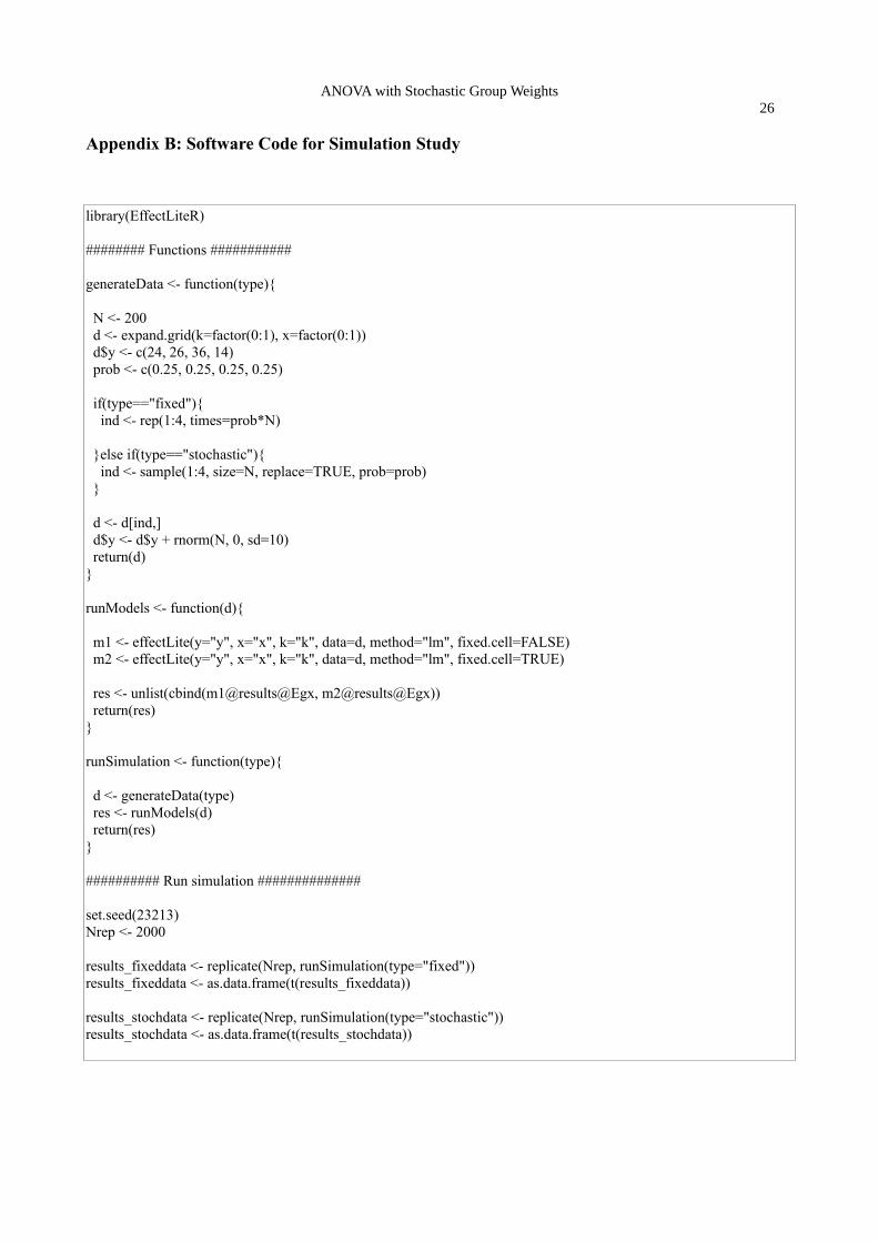
Appendix B: Software Code for Simulation Study
library(EffectLiteR)
######## Functions ###########
generateData <- function(type){ N <- 200 d <- expand.grid(k=factor(0:1), x=factor(0:1)) d$y <- c(24, 26, 36, 14) prob <- c(0.25, 0.25, 0.25, 0.25) if(type=="fixed"){ ind <- rep(1:4, times=prob*N) }else if(type=="stochastic"){ ind <- sample(1:4, size=N, replace=TRUE, prob=prob) } d <- d[ind,] d$y <- d$y + rnorm(N, 0, sd=10) return(d)}
runModels <- function(d){ m1 <- effectLite(y="y", x="x", k="k", data=d, method="lm", fixed.cell=FALSE) m2 <- effectLite(y="y", x="x", k="k", data=d, method="lm", fixed.cell=TRUE) res <- unlist(cbind(m1@results@Egx, m2@results@Egx)) return(res)}
runSimulation <- function(type){ d <- generateData(type) res <- runModels(d) return(res)}
########## Run simulation ##############
set.seed(23213)Nrep <- 2000
results_fixeddata <- replicate(Nrep, runSimulation(type="fixed"))results_fixeddata <- as.data.frame(t(results_fixeddata)) results_stochdata <- replicate(Nrep, runSimulation(type="stochastic"))results_stochdata <- as.data.frame(t(results_stochdata))

ANOVA with Stochastic Group Weights27
Appendix C: Simulation 1
Table C1
Population means and proportions in parentheses for five different scenarios for interactions used
in the first simulation study.
No Interaction Small Interaction Medium Interaction
K=0 K=1 K=2 K=0 K=1 K=2 K=0 K=1 K=2
X=0 40 20 70 36 24 74 32 28 78 (0.5)
X=1 40 20 70 44 16 66 48 12 62 (0.5)
(0.5) (0.1) (0.4) (0.5) (0.1) (0.4) (0.5) (0.1) (0.4)
CE10(K=k) 0 0 0 8 -8 -8 16 -16 -16
AVE10 0 0 0
ηX:K2 0 0.04 0.14
ηpar ; X : K2 0 0.14 0.39
Large Interaction Very Large Interaction
K=0 K=1 K=2 K=0 K=1 K=2
X=0 28 32 82 24 36 86 (0.5)
X=1 52 8 58 56 4 54 (0.5)
(0.5) (0.1) (0.4) (0.5) (0.1) (0.4)
CE10(K=k) 24 -24 -24 32 -32 -32
AVE10 0 0
ηX:K2 0.27 0.39
ηpar ; X : K2 0.59 0.72
Note. The table shows the conditional expectations of Y in the six cells of the 2 x 3 between subject design. Data were generated with normally distributed residuals in each cell with a standard deviation of 10. The average effect is always zero and the adjusted means for both X and K remain constant. The size of the interaction is varied in the five scenarios. ηX :K
2 stands for the effect size of the interaction term.
ANOVA with Stochastic Group Weights28
Figure C1. Type I error rates in the first simulation study. We varied data generation (fixed, stochastic), sample size (100, 200, 500), and size of interaction (no, small, medium, large, very large). Five models were analyzed: A multigroup structural equation model with stochastic group weights (elr_sem_sto), a multigroup structural equation model with fixed group weights (elr_sem_fix), a general linear model with stochastic group weights (elr_lm_sto), a general linear model with fixed group weights (elr_lm_fix), and estimated marginal means which are also based on the general linear model with fixed group weights (emmeans).
ANOVA with Stochastic Group Weights29
Appendix D: Simulation 2
Table D1
Population means and proportions in parentheses for sixteen different scenarios used in the second
simulation study.
No Interaction P(K=0)=0.1
No InteractionP(K=0)=0.2
No InteractionP(K=0)=0.4
No InteractionP(K=0)=0.5
K=0 K=1 K=0 K=1 K=0 K=1 K=0 K=1
X=0 30 20 30 20 30 20 30 20 (0.5)
X=1 30 20 30 20 30 20 30 20 (0.5)
(0.1) (0.9) (0.2) (0.8) (0.4) (0.6) (0.5) (0.5)
ηX:K2 0 0 0 0
ηpar ; X : K2 0 0 0 0
Small Interaction P(K=0)=0.1
Small Interaction P(K=0)=0.2
Small Interaction P(K=0)=0.4
Small Interaction P(K=0)=0.5
K=0 K=1 K=0 K=1 K=0 K=1 K=0 K=1
X=0 21 21 24 21.5 27 22 27 23 (0.5)
X=1 39 19 36 18.5 33 18 33 17 (0.5)
(0.1) (0.9) (0.2) (0.8) (0.4) (0.6) (0.5) (0.5)
ηX:K2 0.08 0.07 0.05 0.07
ηpar ; X : K2 0.08 0.08 0.06 0.08
Large Interaction P(K=0)=0.1
Large Interaction P(K=0)=0.2
Large Interaction P(K=0)=0.4
Large Interaction P(K=0)=0.5
K=0 K=1 K=0 K=1 K=0 K=1 K=0 K=1
X=0 12 22 18 23 24 24 24 26 (0.5)
X=1 48 18 42 17 36 16 36 14 (0.5)
(0.1) (0.9) (0.2) (0.8) (0.4) (0.6) (0.5) (0.5)
ηX:K2 0.25 0.24 0.16 0.22
ηpar ; X : K2 0.26 0.26 0.19 0.27
Very Large Int. P(K=0)=0.1
Very Large Int. P(K=0)=0.2
Very Large Int. P(K=0)=0.4
Very Large Int. P(K=0)=0.5
K=0 K=1 K=0 K=1 K=0 K=1 K=0 K=1
X=0 3 23 12 24.5 21 26 21 29 (0.5)
X=1 57 17 48 15.5 39 14 39 11 (0.5)
(0.1) (0.9) (0.2) (0.8) (0.4) (0.6) (0.5) (0.5)
ηX:K2 0.43 0.41 0.30 0.39
ηpar ; X : K2 0.45 0.45 0.35 0.45
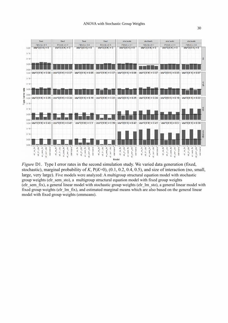
ANOVA with Stochastic Group Weights30
Figure D1. Type I error rates in the second simulation study. We varied data generation (fixed, stochastic), marginal probability of K, P(K=0), (0.1, 0.2, 0.4, 0.5), and size of interaction (no, small,large, very large). Five models were analyzed: A multigroup structural equation model with stochastic group weights (elr_sem_sto), a multigroup structural equation model with fixed group weights (elr_sem_fix), a general linear model with stochastic group weights (elr_lm_sto), a general linear model withfixed group weights (elr_lm_fix), and estimated marginal means which are also based on the general linear model with fixed group weights (emmeans).

ANOVA with Stochastic Group Weights31
Appendix E: Simulation 3
Table E1
Population means and proportions in parentheses for scenarios used in the third simulation study.
Zero Average Effects for K(Low R2)
Non-Zero Average Effects for K(High R2)
K1=0 K1=1 K1=0 K1 =1
K2=0 K2=1 K2=0 K2=1 K2=0 K2=1 K2=0 K2=1
(K=0) (K=1) (K=2) (K=3) (K=0) (K=1) (K=2) (K=3)
X=0 50 50 50 50 30 50 70 90 (0.33)
X=1 70 30 70 30 50 30 90 70 (0.33)
X=2 30 70 30 70 10 70 50 110 (0.33)
(0.3) (0.2) (0.2) (0.3) (0.3) (0.2) (0.2) (0.3)
SD(ε) = 40 ηX:K2 0.73 0.28 Very
LargeInt.SD(ε) = 40 ηpar ; X : K
2 0.73 0.73
SD(ε) = 20 ηX:K2 0.40 0.21 Large
Int.SD(ε) = 20 ηpar ; X : K
2 0.40 0.40
SD(ε) = 10 ηX:K2 0.14 0.11 Small
Int.SD(ε) = 10 ηpar ; X: K
2 0.14 0.14
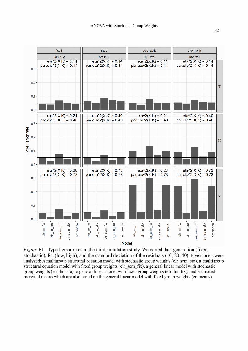
ANOVA with Stochastic Group Weights32
Figure E1. Type I error rates in the third simulation study. We varied data generation (fixed, stochastic), R2, (low, high), and the standard deviation of the residuals (10, 20, 40). Five models wereanalyzed: A multigroup structural equation model with stochastic group weights (elr_sem_sto), a multigroupstructural equation model with fixed group weights (elr_sem_fix), a general linear model with stochastic group weights (elr_lm_sto), a general linear model with fixed group weights (elr_lm_fix), and estimated marginal means which are also based on the general linear model with fixed group weights (emmeans).
ANOVA with Stochastic Group Weights33
Appendix F: Simulation 4
Table F1
Scenarios used in the fourth simulation study.
No InteractionP(X=0)=0.5
No InteractionP(X=0)=0.2
K=0 K=1 K=0 K=1
X=0 30 20 (0.5) 30 20 (0.2)
X=1 30 20 (0.5) 30 20 (0.8)
(0.5) (0.5) (0.5) (0.5)
ηX:K2 0 / 0 0 / 0
ηpar ; X : K2 0 / 0 0 / 0
Small Interaction P(X=0)=0.5
Small Interaction P(X=0)=0.2
K=0 K=1 K=0 K=1
X=0 27 23 (0.5) 27 23 (0.2)
X=1 33 17 (0.5) 33 17 (0.8)
(0.5) (0.5) (0.5) (0.5)
ηX:K2 0.07 / 0.06 0.04 / 0.02
ηpar ; X : K2 0.08 / 0.07 0.06 / 0.03
Large Interaction P(X=0)=0.5
Large Interaction P(X=0)=0.2
K=0 K=1 K=0 K=1
X=0 24 26 (0.5) 24 26 (0.2)
X=1 36 14 (0.5) 36 14 (0.8)
(0.5) (0.5) (0.5) (0.5)
ηX:K2 0.22 / 0.19 0.12 / 0.08
ηpar ; X : K2 0.26 / 0.22 0.19 / 0.11
Very Large Int. P(X=0)=0.5
Very Large Int. P(X=0)=0.2
K=0 K=1 K=0 K=1
X=0 21 29 (0.2) 21 29 (0.2)
X=1 39 11 (0.8) 39 11 (0.8)
(0.5) (0.5) (0.5) (0.5)
ηX:K2 0.39 / 0.35 0.20 / 0.15
ηpar ; X : K2 0.45 / 0.39 0.34 / 0.22
Note. Effect sizes for interactions are given for homogeneous / heterogeneous residual variances.
ANOVA with Stochastic Group Weights34
Figure F1. Type I error rates in the fourth simulation study. We varied data generation (fixed, stochastic), structure of residual variances, (homogenous, heterogenous), group sizes for X (equal, unequal), and the size of the interaction (no, small, large, very large). Five models were analyzed: A multigroup structural equation model with stochastic group weights (elr_sem_sto), a multigroup structural equation model with fixed group weights (elr_sem_fix), a general linear model with stochastic group weights(elr_lm_sto), a general linear model with fixed group weights (elr_lm_fix), and estimated marginal means which are also based on the general linear model with fixed group weights (emmeans).
ANOVA with Stochastic Group Weights35
Appendix G: Simulation 5
Table G1
Scenarios used in the fifth simulation study.
No Interaction
Cor(X, K) = 0 Cor(X, K) = 0.2 Cor(X, K) = 0.6
K=0 K=1 K=0 K=1 K=0 K=1
X=0 30(0.25)
20(0.25)
(0.5) 30(0.3)
20(0.2)
(0.5) 30(0.4)
20(0.1)
(0.5)
X=1 30(0.25)
20(0.25)
(0.5) 30(0.2)
20(0.3)
(0.5) 30(0.1)
20(0.4)
(0.5)
(0.5) (0.5) (0.5) (0.5) (0.5) (0.5)
Small Interaction
Cor(X, K) = 0 Cor(X, K) = 0.2 Cor(X, K) = 0.6
K=0 K=1 K=0 K=1 K=0 K=1
X=0 27(0.25)
23(0.25)
(0.5) 27(0.3)
23(0.2)
(0.5) 27(0.4)
23(0.1)
(0.5)
X=1 33(0.25)
17(0.25)
(0.5) 33(0.2)
17(0.3)
(0.5) 33(0.1)
17(0.4)
(0.5)
(0.5) (0.5) (0.5) (0.5) (0.5) (0.5)
Large Interaction
Cor(X, K) = 0 Cor(X, K) = 0.2 Cor(X, K) = 0.6
K=0 K=1 K=0 K=1 K=0 K=1
X=0 24(0.25)
26(0.25)
(0.5) 24(0.3)
26(0.2)
(0.5) 24(0.4)
26(0.1)
(0.5)
X=1 36(0.25)
14(0.25)
(0.5) 36(0.2)
14(0.3)
(0.5) 36(0.1)
14(0.4)
(0.5)
(0.5) (0.5) (0.5) (0.5) (0.5) (0.5)
Very Large Interaction
Cor(X, K) = 0 Cor(X, K) = 0.2 Cor(X, K) = 0.6
K=0 K=1 K=0 K=1 K=0 K=1
X=0 21(0.25)
29(0.25)
(0.2) 21(0.3)
29(0.2)
(0.5) 21(0.4)
29(0.1)
(0.5)
X=1 39(0.25)
11(0.25)
(0.8) 39(0.2)
11(0.3)
(0.5) 39(0.1)
11(0.4)
(0.5)
(0.5) (0.5) (0.5) (0.5) (0.5) (0.5)Note. Cell and marginal proportions are given in parentheses.

ANOVA with Stochastic Group Weights36
Figure G1. Type I error rates in the fifth simulation study. We varied data generation (fixed, stochastic), the correlation between X and K (no=0 (independent), small=0.2, large=0.6), and the size of the interaction (no, small, large, very large). Five models were analyzed: A multigroup structural equation model with stochastic group weights (elr_sem_sto), a multigroup structural equation model with fixed group weights (elr_sem_fix), a general linear model with stochastic group weights (elr_lm_sto), a general linear model with fixed group weights (elr_lm_fix), and estimated marginal means which are also based on the general linear model with fixed group weights (emmeans).