228

© Taylor & Francis

Chapter 12

Repeated-Measures ANOVA

12.1 Visualizing Data with Interaction (Means) Plots and Parallel Coordinate Plots

12.1.1 Creating Interaction (Means) Plots in R with More Than One Response Variable

Interaction or means plots using the plotMeans() command were covered in the online document ―Factorial ANOVA.Visual summary with means plots,‖ but I noted there that this command cannot deal with more than one response variable at a time. The interaction.plot() command can deal with more than one response variable, but you may have to massage your data into a different format for the plot to work. I reiterate that interaction plots in general are relatively information-poor plots, but they can be useful for getting the big picture of what is going on with your data, so I will explain here how to make interaction.plot() work with the Murphy (2004) data. The data needs to be in the ―long‖ form, where all of the numerical scores are concatenated into one column, with index columns specifying the categories the data belongs to. Murphy’s (2004) data in its original form was set up to easily perform an RM ANOVA in SPSS (this is called the ―wide‖ form), which means it is not in the correct form for making an interaction plot in R (or for doing the repeated-measures analysis in R either). Murphy’s (2004) original data set, with performance on each of the six verb categories in separate columns, is shown in Figure 12.1. This data set is only 60 columns long.

Figure 12.1 Murphy (2004) data in original form. The online section ―Repeated measures ANOVA.Putting data in correct format for RM ANOVA‖ explains how to put Murphy’s data into the correct form for the interaction plot and the RM ANOVA (the ―long‖ form). After manipulation, Murphy’s data has one column with the score (verbs), one column to note which of the three groups the participant belongs

229

© Taylor & Francis

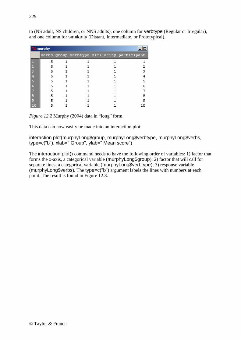
to (NS adult, NS children, or NNS adults), one column for verbtype (Regular or Irregular), and one column for similarity (Distant, Intermediate, or Prototypical).

Figure 12.2 Murphy (2004) data in ―long‖ form. This data can now easily be made into an interaction plot:

interaction.plot(murphyLong$group, murphyLong$verbtype, murphyLong$verbs, type=c("b"), xlab=" Group", ylab=" Mean score") The interaction.plot() command needs to have the following order of variables: 1) factor that forms the x-axis, a categorical variable (murphyLong$group); 2) factor that will call for separate lines, a categorical variable (murphyLong$verbtype); 3) response variable (murphyLong$verbs). The type=c("b") argument labels the lines with numbers at each point. The result is found in Figure 12.3.

230

© Taylor & Francis

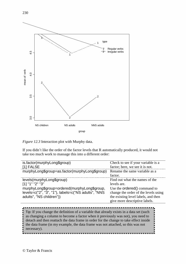
Figure 12.3 Interaction plot with Murphy data. If you didn’t like the order of the factor levels that R automatically produced, it would not take too much work to massage this into a different order:

is.factor(murphyLong$group) [1] FALSE

Check to see if your variable is a factor; here, we see it is not.

murphyLong$group=as.factor(murphyLong$group) Rename the same variable as a factor.

levels(murphyLong$group) [1] "1" "2" "3"

Find out what the names of the levels are.

murphyLong$group=ordered(murphyLong$group, levels=c("2", "3", "1"), labels=c("NS adults", "NNS adults", "NS children"))

Use the ordered() command to change the order of the levels using the existing level labels, and then give more descriptive labels.

1

1

1

3.0

3.5

4.0

4.5

group

me

an

of v

erb

2

2

2

NS children NS adults NNS adults

type

12

Regular verbsIrregular verbs

Tip: If you change the definition of a variable that already exists in a data set (such

as changing a column to become a factor when it previously was not), you need to detach and then reattach the data frame in order for the change to take effect inside the data frame (in my example, the data frame was not attached, so this was not necessary).

231

© Taylor & Francis

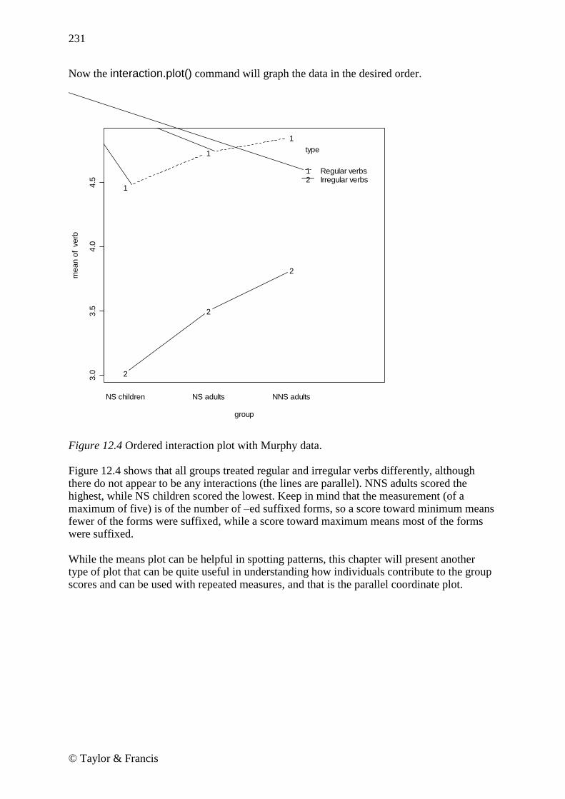
Now the interaction.plot() command will graph the data in the desired order.

Figure 12.4 Ordered interaction plot with Murphy data. Figure 12.4 shows that all groups treated regular and irregular verbs differently, although there do not appear to be any interactions (the lines are parallel). NNS adults scored the highest, while NS children scored the lowest. Keep in mind that the measurement (of a maximum of five) is of the number of –ed suffixed forms, so a score toward minimum means fewer of the forms were suffixed, while a score toward maximum means most of the forms were suffixed. While the means plot can be helpful in spotting patterns, this chapter will present another type of plot that can be quite useful in understanding how individuals contribute to the group scores and can be used with repeated measures, and that is the parallel coordinate plot.

1

1

1

3.0

3.5

4.0

4.5

group

me

an

of v

erb

2

2

2

NS children NS adults NNS adults

type

12

Regular verbsIrregular verbs

232

© Taylor & Francis

12.1.2 Parallel Coordinate Plots

A very nice graphic that takes the place of the means plot and contains many more points of data is the parallel coordinate plot (sometimes called a profile plot). Adamson and Bunting (2005) say that a profile plot can help viewers get a general impression of the trends of individuals that go into a means plot. An example of a profile plot for the Lyster (2004) data is seen in Figure 12.5. This shows the performance of individuals in the four different conditions over the three times participants were tested (pre-test, immediate post-test, and delayed post-test) on the written completion task (cloze). The graphic shows a line representing each individual, and separate panels are given for the participants within each treatment group. Considering that the further to the right in the panel a score is the higher it is, a leaning to the right in a line indicates that the learner has improved on their ability to use French gender correctly for this task. We see a very strong trend toward learning for the FFI Prompt group in the immediate post-test (Post1TaskCompl), although this attenuates in the delayed post-test (Post2TaskCompl). There also seems to be some general movement to the right in both the FFI Recast and FFI Only groups, although we can see some individuals who get worse in the post-tests. In the comparison group the individual movement of lines from pre-test to post-test seems very random.

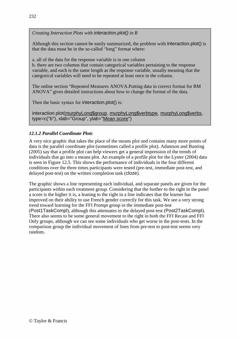
Creating Interaction Plots with interaction.plot() in R Although this section cannot be easily summarized, the problem with interaction.plot() is that the data must be in the so-called ―long‖ format where: a. all of the data for the response variable is in one column b. there are two columns that contain categorical variables pertaining to the response variable, and each is the same length as the response variable, usually meaning that the categorical variables will need to be repeated at least once in the column. The online section ―Repeated Measures ANOVA.Putting data in correct format for RM ANOVA‖ gives detailed instructions about how to change the format of the data. Then the basic syntax for interaction.plot() is:

interaction.plot(murphyLong$group, murphyLong$verbtype, murphyLong$verbs, type=c("b"), xlab="Group", ylab="Mean score")

233

© Taylor & Francis

Figure 12.5 Profile plot of data for Lyster (2004). The syntax for creating a parallel plot is quite simple. I imported the Lyster.written.sav file.

library(lattice) attach(lyster) parallel(~lyster[6:8] | lyster$Cond) parallel (x, . . . ) Command for parallel coordinate plot; x should be a data

frame or matrix, as the Lyster data set is.

(~lyster[6:8] The name of the matrix is lyster, and the brackets enclose the three columns of the matrix that should be used.

| Cond The vertical line (found by using the Shift key plus backslash) precedes the conditioning variable, in this case the condition (Cond).

PreTaskCompl

Post1TaskCompl

Post2TaskCompl

Min Max

FFIrecast FFIprompt

PreTaskCompl

Post1TaskCompl

Post2TaskCompl

FFIonly

Min Max

Comparison

234

© Taylor & Francis

It is also possible to easily split the output with another variable. For example, in the data from Chapter 11 by Obarow, a parallel coordinate plot could be done showing the change from the immediate post-test to the delayed post-test according to each of the four conditions (we can do this because Obarow tested over more than one time period, thus providing the data for a repeated-measures study, even though we ignored the variable of time in Chapter 11). However, that study also found a statistical difference for gender, so we could include this variable to split each of the four conditions (see Figure 12.6).

Figure 12.6 Parallel coordinate plot for Obarow Story 1. The syntax for adding another variable is just to connect it using the asterisk (―*‖).

parallel(~obarow[8:9]|obarow$Treatment1*obarow$gender) If this is extended to three variables, which is possible, R will print two different pages of R graphics, split by the last variable in your list. For example, the command:

gnsc1.1

gnsc1.2

Min Max

No music No pics

male

No music Yes pics

male

Min Max

Yes music No pics

male

Yes music Yes pics

male

gnsc1.1

gnsc1.2

No music No pics

female

Min Max

No music Yes pics

female

Yes music No pics

female

Min Max

Yes music Yes pics

female

235

© Taylor & Francis

parallel(~obarow[8:9]|obarow$PicturesT1*obarow$MusicT1*obarow$gender) will give one page of graphics with just the females split by pictures and music, and another page of graphics with just the males split by pictures and music (try it!).

12.2 Application Activities for Interaction (Means) Plots and Parallel Coordinate Plots

1. Create a means plot with Lyster’s (2004) data. Import the SPSS file LysterClozeLong.sav and save it as lysterMeans. Lyster had four experimental groups (―Cond‖) over three time periods (―Time‖) for the written cloze task measured here (―ClozeTask‖). The data have already been arranged in the long form. Create a means plot with the three time periods as the separate lines, and the four groups as categories on the x-axis. Which group received the highest mean score on the immediate post-test? Which group received the highest mean score on the delayed post-test? Do you see any parallel trends in the means plot? Which groups made gains and which did not? How does this plot compare to the parallel coordinate plot in Figure 12.5? 2. Larson-Hall (2004) data. Create a means plot by first importing the LarsonHall2004MeansPlot.sav file and calling it LHMeans. In this study Japanese learners of Russian were tested for repeated measures on phonemic contrasts, but the original data has been cut down to just three contrasts (R_L, SH_SHCH, F_X). The data has already been arranged in the long form. Make a means plot where the separate lines are the three contrasts (―contrast‖). Now try to make a means plot where separate lines are the four groups (―level‖). Describe the means plots you can make. 3. Lyster (2004) data. Import the Lyster.Written.sav file as lyster. Create a parallel coordinate plot for the written binary task in the Lyster data set. Use the variables PreBinary, Post1Binary and Post2Binary and split the data by the variable of condition (Cond). Describe what the plots show about how each group performed. 4. Murphy (2004) data. Create a parallel coordinate plot for the Murphy (2004) data set (using the ―wide‖ form of the Murphy data set; if you have already imported the Murphy.sav SPSS file as murphy you can just use this data set). Examine how participants performed with regular verbs, with data split into the three different groups of participants. Then look at a parallel coordinate plot for the irregular verbs. Do the participants seem to have parallel patterns? Keep in mind that the measurement is of the number of –ed suffixed forms, so a score toward minimum means fewer of the forms were suffixed while a score toward maximum means most of the forms were suffixed. 12.3 Putting Data in the Correct Format for RM ANOVA

Creating Parallel Coordinate Plots The basic command in R is:

library(lattice) parallel(~lyster[6:8] | lyster$Cond) or

parallel(~obarow[8:9]|obarow$Treatment1*obarow$gender) where the data needs to be in a data frame or matrix so that columns can be selected for the first argument of the command.

236

© Taylor & Francis

Data for any type of linear modeling in R (whether regression, ANOVA, or mixed-effects) needs to be arranged in ―long‖ form, which means that all of the data for the response variable needs to be in one column. There will then be index columns that specify the categorical distinctions for the fixed-effect and random-effect variables. Murphy’s (2004) original data set is arranged in the proper format to do an RM ANOVA in SPSS (see Figure 12.7); therefore, it will need to be reconfigured for R. In the original data set there are 60 participants with six recorded pieces of information each (participants’ scores on the 30-item wug test have been divided into categories depending on regular/irregular verb type and prototypical/intermediate/distant similarity to real verbs). This means we will want one (60×6=) 360-item column along with four indexing columns: one for the participants themselves (since the participants’ data will take up more than one row, we need to know which rows all belong to the same person), one for the between-group category the entry belongs to (NS adult, NS child, or NNS adult), one for verb type, and one for verb similarity.

Figure 12.7 Murphy (2004) data in original form. The following table will walk you through the steps in R for converting Murphy’s (2004) data from a ―short‖ form into a ―long‖ form (I will start with the imported SPSS file Murphy.sav which has been called ―murphy‖ and convert it into murphyLong).

names(murphy) [1] "group" "RegProto" [3] "RegInt" "RegDistant" [5] "IrregProto" "IrregInt" [7] "IrregDistant"

Find out names of the columns; group is a categorical variable specifying which of three categories the participants fit in.

murphyLong<- stack(murphy [,c("RegProto", "RegInt", "RegDistant", "IrregProto", "IrregInt", "IrregDistant")])

stack takes all the numerical values and concatenates them into one long column which is indexed by column names, and we specify which columns to choose.

names(murphyLong) <- c("verbs", "index")

I’ve named the two columns in the new data frame.

levels(murphy$group) [1] "NS children" "NS adults" "NNS adults"

The next step is to make an index column specifying which group each entry belongs to. In order to do this, I first ask for the names (and implicit order) of the original variable, group.

group=gl(3,20,360,labels= c("NS children", "NS adults", "NNS adults"))

The gl command stands for ―generate levels‖ and creates a factor whose

237

© Taylor & Francis

arguments are: 1) number of levels; 2) how many times each level should repeat; 3) total length of result; and 4) labels for levels; note that number 2 works only if the number of subjects in each group is exactly the same!

participant=factor(rep(c(1:60),6)) Generates an index so that each item is labeled as to the participant who produced it (because there were 60 separate rows for each original variable, and these were 60 separate individuals).

verbtype=gl(2,180,360,labels=c("regular", "irregular"))

Generates an index of verb type (regular vs. irregular).

similarity=rep(rep(1:3,c(20,20,20)),6)

For verb similarity, instead of using gl I use rep to demonstrate how this factor could be called for if you had different numbers of groups in each category; the rep command works like this: 1:3 specifies to insert the numbers ―1,‖ ―2,‖ ―3‖; the c(20,20,20) specifies the times that each number (1, 2, or 3) should be repeated; the 6 specifies that this whole sequence should be repeated 6 times (this applies to the outer rep command).

similarity=as.factor(similarity)

The rep command does not create a factor, so we do that here.

levels(similarity)=c("prototypical", "intermediate", "distant")

Give the similarity levels names here.

murphyLong=data.frame(cbind(verbs= murphyLong$verbs, group, verbtype, similarity, participant))

Collect all of the vectors just created and put them together into a data frame; notice that for all but the first column the name will be the name of the vector, but for the first one I specify the name I want.

str(murphyLong) This command will tell you about the structure of the data frame. You might use this to verify that the variables that are factors are marked as factors. Even though I made all of the variables that were factors into factors, they are not factors after I bind them, so I go through the steps again.

murphyLong$group=as.factor(murphyLong$group) levels(murphyLong$group)=c("NS children", "NS adults", "NNS adults")

Make group into a factor and label levels.

murphyLong$verbtype=as.factor(murphyLong$verbtype) levels(murphyLong$verbtype)= c("regular", "irregular")

Make verb type into a factor and label levels.

murphyLong$similarity=as.factor(murphy Make similarity into a factor and label

238

© Taylor & Francis

Long$similarity) levels(murphyLong$similarity)= c("prototypical", "intermediate", "distant")

levels.

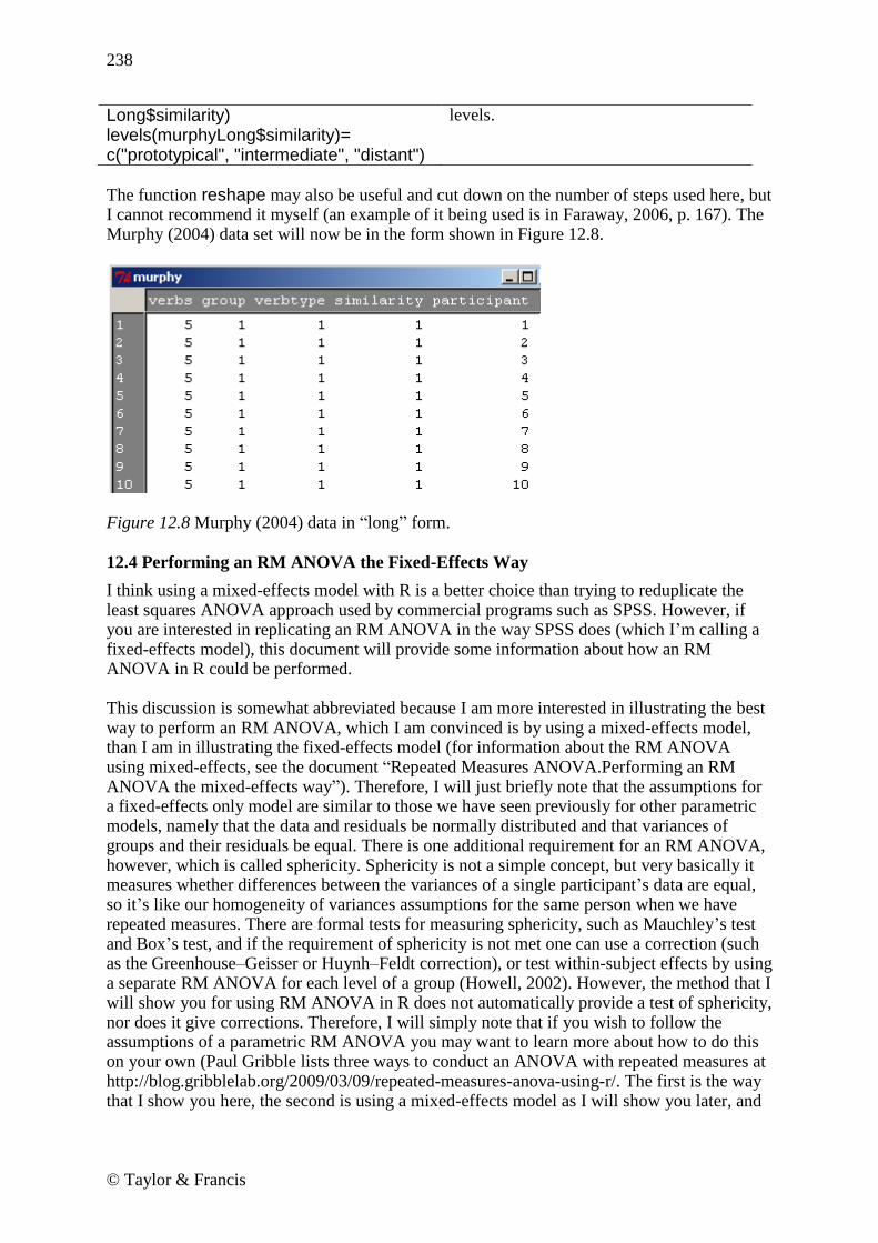
The function reshape may also be useful and cut down on the number of steps used here, but I cannot recommend it myself (an example of it being used is in Faraway, 2006, p. 167). The Murphy (2004) data set will now be in the form shown in Figure 12.8.

Figure 12.8 Murphy (2004) data in ―long‖ form. 12.4 Performing an RM ANOVA the Fixed-Effects Way

I think using a mixed-effects model with R is a better choice than trying to reduplicate the least squares ANOVA approach used by commercial programs such as SPSS. However, if you are interested in replicating an RM ANOVA in the way SPSS does (which I’m calling a fixed-effects model), this document will provide some information about how an RM ANOVA in R could be performed. This discussion is somewhat abbreviated because I am more interested in illustrating the best way to perform an RM ANOVA, which I am convinced is by using a mixed-effects model, than I am in illustrating the fixed-effects model (for information about the RM ANOVA using mixed-effects, see the document ―Repeated Measures ANOVA.Performing an RM ANOVA the mixed-effects way‖). Therefore, I will just briefly note that the assumptions for a fixed-effects only model are similar to those we have seen previously for other parametric models, namely that the data and residuals be normally distributed and that variances of groups and their residuals be equal. There is one additional requirement for an RM ANOVA, however, which is called sphericity. Sphericity is not a simple concept, but very basically it measures whether differences between the variances of a single participant’s data are equal, so it’s like our homogeneity of variances assumptions for the same person when we have repeated measures. There are formal tests for measuring sphericity, such as Mauchley’s test and Box’s test, and if the requirement of sphericity is not met one can use a correction (such as the Greenhouse–Geisser or Huynh–Feldt correction), or test within-subject effects by using a separate RM ANOVA for each level of a group (Howell, 2002). However, the method that I will show you for using RM ANOVA in R does not automatically provide a test of sphericity, nor does it give corrections. Therefore, I will simply note that if you wish to follow the assumptions of a parametric RM ANOVA you may want to learn more about how to do this on your own (Paul Gribble lists three ways to conduct an ANOVA with repeated measures at http://blog.gribblelab.org/2009/03/09/repeated-measures-anova-using-r/. The first is the way that I show you here, the second is using a mixed-effects model as I will show you later, and

239

© Taylor & Francis

the third way involves restructuring the data to use the Anova() command in the car library, which will then return a sphericity value and corrections). An RM ANOVA can be performed in R by using an aov() linear model and adding an ―Error‖ term that contains the ―subjects‖ term, plus the within-subjects variables with variables listed from largest to smallest if there is any hierarchy to the data (Baron & Li, 2003; Crawley, 2007; Revelle, 2005). For example, recall that, for the Murphy (2004) data, we are asking whether verb type, verb similarity, and age/NS status (in the ―group‖ variable) affect how often participants attach the regular past tense [–ed] ending. The response variable is verbs. The variables verbtype, similarity, and group are categorical explanatory variables. Two are within-subject variables (verbtype and similarity), and one is a between-subject variable (group). We will put only the within-subject variables in the ―Error‖ section of the model, not the between-subject variable. In order for this modeling to work properly, it is very important that your data have the correct structure. Check the structure with the str() command, and make sure all of your categorical variables are factors as well as your subject or participant variable. str(murphyLong)

If your participant variable is not a factor then make it one (it won’t be in the file you import from SPSS):

murphyLong$participant=as.factor(murphyLong$participant) In the Murphy data set, the subjects are called ―participant.‖ To make sure you have the correct set-up for this analysis (if you are following along with me), import the SPSS file called MurphyLongForm.sav and call it murphyLong. Now we can model:

murphy.aov=aov(verbs~(verbtype*similarity*group)+ Error(participant/verbtype*similarity),data=murphyLong) summary(murphy.aov) The following table gives the syntax that would be used for differing numbers of within-subject and between-subject variables (Revelle, 2005).

1.1.1.1.1.1.1.1 Number of Within-Subject Variabl

1.1.1.1.1.1.1.2 Number of Between-Subject

1.1.1.1.1.1.1.3 Model Formula

240

© Taylor & Francis

es Variables

1 0 aov(DV~IV + Error (Subject/IV), data=data)

2 0 aov(DV~IV*IV + Error (Subject/IV*IV), data=data)

3 0 aov(DV~IV*IV*IV + Error(Subject/(IV*IV*IV)), data=data)

2 1 aov(DV~~(IVbtw*IV*IV) + Error(Subject/( IV*IV)), data=data)

2 2 aov(DV~~(IVbtw* IVbtw *IV*IV) + Error(Subject/( IV*IV)) , data=data)

The pattern is clear—within-subject variables are entered in the error term as well as in the non-error term, but between-subject variables need only be entered once. Note that, if you are working with data in a ―wide‖ or ―short‖ form in R, you will need to create your own ―participant‖ column in order to keep track of which participant is linked to which piece of data. Note also that it actually doesn’t matter whether the between-subject variables come before or after the within-subject variables (I ran my analysis with the between-subject variable of group after the within-subject variables). Returning now to the output of the repeated-measures model, we have the following output:

241

© Taylor & Francis

The output provides quite a bit of information, which can be overwhelming at first. All of the information after the first grouping (labeled ―Error: participant‖) concerns the within-subjects effects, but the first grouping concerns the between-subjects effect. Here we have only one between-subjects variable, that of group, and so we can see that the effect of group is statistical because the p-value, found in the column labeled ―Pr(>F),‖ is less than .05. We will want to note a couple more pieces of information about this interaction, which are the F-value and the degrees of freedom, and report that the main effect of group was statistical (F2,57=5.67, p=.006, partial eta-squared=(2*5.67/ ((2*5.67) +57) =.17).

1

For the within-subject effects there are basically three groupings: those dealing with verbtype, those dealing with similarity, and those dealing with the interaction between verbtype and similarity. The report for similarity is split into two sections (labeled ―Error: similarity‖ and ―Error: participant:similarity‖) depending on what error term is in the denominator, but they both concern the effect of similarity. Remember, one of the features of repeated measures is that, instead of using the same error term as the denominator for every entry in the ANOVA table, an RM ANOVA is able to use different (appropriate) error terms as denominators and thus factor out subject differences. In R these error terms are the row labeled ―Residuals.‖ I advise researchers to look first at the largest interactions and then work backwards, since main effects for single variables may not retain their importance in the face of the interactions. The largest interaction is the three-way interaction between type of verb, similarity of verb, and group, which is the last entry in the output printed here (labeled ―Error: participant: verbtype: similarity‖). This is a statistical interaction (F4,114=3.28, p=.01, partial eta-squared=4*3.28/((4*3.28)+114)=.10) with a medium effect size. What this means is that participants from the different groups performed differently on regular and irregular verbs, and they also performed differently on at least one of the types of similarities of verbs. In other words, the groups did not all perform in a parallel manner on both types of verbs and all three types of verb similarities. The process of understanding the output is the same for other interactions and main effects listed in the output. Howell (2002) notes that researchers should not feel compelled to report every statistical effect that they find, feeling they must do so for the sake of completeness. In addition, Kline (2004) observes that non-statistical effects may be at least as interesting as, if not more interesting than, statistical effects. One important point to consider is the effect size. If a certain comparison has an effect size that is noteworthy but the comparison is not statistical, this may be due to insufficient power (probably owing to a small group size), and further testing with larger groups would probably uncover a statistical relationship. If this information could further hypotheses, then it should probably be reported. In an RM ANOVA you are sure to have large amounts of output, so consider carefully what your questions are and what data you would like to report. Going through the rest of the output, we can see that there is a statistical main effect for verb type with a large effect size (F1,57=233.24, p<.0001, partial eta-squared=.80). The main effect for similarity does not include an F value or a p-value, but we can calculate the F by dividing the mean square of similarity by the mean square of the error (Residual) term for similarity (found in the grouping ―Error: participant:similarity‖), which would be 16.19/.42=38.5, which is a very large F and would certainly be statistical (using the SPSS print-out of the

1 Note that I am using the equation

2

22

1

f to calculate effect size.

242

© Taylor & Francis

same analysis I find a statistical main effect for similarity, F2,114=38.22, p<.0001, partial eta-squared=.40). The interaction between verbtype and group is not statistical (F2,57=2.20, p=.12, partial eta-squared=.07), but the interaction between similarity and group is (F4,114=3.94, p=.005, partial eta-squared=.12), and so is the interaction between verbtype and similarity (F2,114=62.63, p<.0001, partial eta-squared=.52). At this point we still have some unanswered questions because, since there are more than two levels of variables involved in the variables in the interaction, we don’t yet understand the nature of the interaction. For example, is the difference between verb similarities statistical for all three groups of participants? Is the difference between verb regularity statistical across all three similarities of verbs? Some of these questions we can answer based on data already contained in the output, but some we will have to do some extra work to request. However, keep in mind that results that are pertinent to the theoretical hypotheses and address the issues the researcher wants to illuminate are the right choice for reporting. For the Murphy (2004) data, let us look at the hypotheses Murphy formulated and, knowing that there is a statistical three-way interaction, decide which further comparisons to look at. Murphy’s (2004) hypotheses were:

1. All groups will add more –ed forms to regular verbs than irregular verbs. 2. Similarity should play a role on irregular verbs but not regular verbs. 3. Group differences in amount of suffixed forms should be seen only in the irregular

verbs, not the regular ones. 4. No previous research looked at these three groups, so it is unclear which groups will

pattern together. For hypothesis 1 we could first look at descriptive statistics. A normal call for summary statistics will not get us what we need, however. To get our answer we need to manipulate our data so all of the regular verbs are in one column and all of the irregular verbs are in another column (so each of these columns will have a maximum score of 15 points). This can be done by using the murphy data set and creating a new variable that adds together all of the points of the irregular verbs and then for regular verbs, like this (in R Commander, use Data > Manage variables in active data set > Compute new variable):

murphy$Irregulars <- with(murphy, IrregDistant+ IrregInt+ IrregProto) murphy$Regulars <- with(murphy, RegDistant+ RegInt+ RegProto) Now I call for descriptive statistics separating the scores in these new variables by group membership (in R Commander: Statistics > Summaries > Numerical summaries). The descriptive statistics show in every case that regulars were suffixed more than irregulars (mean scores—NS children: reg.V = 14.6, irreg.V = 11.5; NS adults: reg.V = 13.4, irreg.V = 9.1; NNS adults: reg.V = 14.2, irreg.V = 10.5). We also know there is a statistical difference with a very strong effect size for verbtype from the output above (F1,57=233.24, p<.0001, partial eta-squared=.80), and since there were only two levels for verb type no further analysis is necessary to state that regular verbs received statistically more –ed forms than irregulars, and that all of the participant groups followed this pattern (because there was no interaction between verbtype and group, so it follows that all groups performed in a parallel manner). For hypothesis 2 we would want to see an interaction between similarity and verbtype. This interaction was indeed statistical, again with a large effect size (F2,114=62.63, p<.0001, partial eta-squared=.52). We need to know more about this interaction, and we can use the

243

© Taylor & Francis

pairwise.t.test() command (explained in more detail in the online document ―Factorial ANOVA.Performing comparisons in a factorial ANOVA‖) to look at post-hoc comparisons with the interaction. I don’t want to perform post-hocs comparing the regular verbs to irregular ones, however, just the regular ones to each other, so I specify the rows in order to pick out just the regular verbs first:

pairwise.t.test(murphyLong$verbs[1:180], murphyLong$verbtype[1:180]:murphyLong$similarity[1:180], p.adjust.method="fdr")

The pairwise comparisons show that, for regular verbs, prototypical and intermediate verbs are statistically different from distant verbs (a look at the summary statistics not shown here indicates they are more suffixed than distant verbs; in fact, prototypical and intermediate verbs that are regular have exactly the same mean). This contradicts the hypothesis that similarity plays no role for regular verbs. Repeat the process for irregular verbs only:

pairwise.t.test(murphyLong$verbs[181:360], murphyLong$verbtype[181:360]:murphyLong$similarity[181:360], p.adjust.method="fdr") For irregular verbs (verbtype 2), there are statistical differences between prototypical and distant verbs and also between intermediate and distant verbs. Thus hypothesis 2 is not upheld, because similarity interacts with both types of verbs. Murphy (2004) points out that these effects run in opposite directions; participants suffix least for distant similarity when verbs are regular, but suffix most for distant similarity when verbs are irregular (look back to the means plot in Figure 12.3 to confirm this visually). Hypothesis 3 posited that the groups would suffix differently on the irregular verbs but not on the regular verbs. In other words, there should be an interaction between verbtype and group, but there is none (F2,57=2.2, p=.12, partial eta-squared=.07). The means plots indicate that group differences in the amount of suffixed verbs are present for both regular and irregular verbs. To look in more detail at how the groups performed on both types of verbs, we can run the RM ANOVA analysis again but only put in regular verbs (so there would be only one independent variable of similarity, and we could pick out just the rows that tested regular verbs as in the pairwise t-test above). We would run it again with just the irregular verbs too. Post-hocs will then tell us whether the groups performed differently on the regular verbs (in the first run) and on the irregular verbs (in the second run). In the case of Murphy’s data, where there were two IVs, the RM ANOVA is appropriate, but, in other cases where there is only one IV, further testing would need to be done with a one-way ANOVA.

244

© Taylor & Francis

Doing this for the regular verbs, I found that the variable of group was statistical. Post-hocs showed that children are statistically different from NS adults (p=.03) but not NNS adults, and that NS and NNS adults are not statistically different from one another. For irregular verbs, post-hocs showed exactly the same situation as with regular verbs. Hypothesis 3 is therefore discredited, as there are group differences for both irregular and regular verbs. Note that running a couple more tests beyond the original RM ANOVA to answer a hypothesis (such as I just did for hypothesis 3) does not mean that you need to adjust p-values for everything because you have run too many tests. Howell (2002) has only two cautions in such cases. One is that you not try to include every result from the tests. Just get the results you need and don’t look at the rest. The second caution is that, if you are going to use many more results from such additional testing, then you should adjust the familywise error rate. However, in this case where only a couple of results were investigated, and in fact we did not look at the results of every single comparison, there is no need to adjust the error rate. Hypothesis 4 was concerned about which groups would pattern together. To answer this question we can report there was an overall statistical main effect for group (F2,57=5.7, p=.006, partial eta-squared=.17). We can run post-hoc tests for group using the pairwise.t.test() command. These show that NS children were statistically different from NS adults and NNS adults were statistically different from the NS adults but not children. To summarize then, what steps you will take after running an RM ANOVA will depend on your questions, but hopefully this discussion has helped you see how you might address the questions you have.

12.5 Performing an RM ANOVA the Mixed-Effects Way

You have hopefully look at section 12.4, which shows how to perform a least squares RM ANOVA that replicated the type of model SPSS uses for RM ANOVA. In this section I will demonstrate how to use a mixed-effects model to examine repeated-measures data. 12.5.1 Performing an RM ANOVA

Performing an RM ANOVA with R (Fixed Effects Only) 1. Use an aov() linear model and add an ―Error‖ term that contains the ―subjects‖ term, plus the within-subjects variables with variables listed from largest to smallest if there is any hierarchy to the data. Here is one example for two within-group variables (A and B) and one between-group variable (Group):

model.aov=aov(DepVar~(VarA*VarB*Group)+ Error(Participant/VarA*VarB), data=dataset Examples of other configurations are shown in the text.

2. For this to work properly, make sure all of your independent variables as well as your Participant variable are factors (use str() to ascertain the structure of your data set). 3. Use normal means of assessing linear models, such as summary(model.aov), and normal

reduction of model by looking for the minimal adequate model.

245

© Taylor & Francis

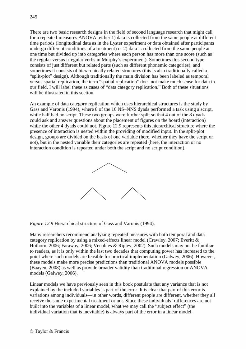
There are two basic research designs in the field of second language research that might call for a repeated-measures ANOVA: either 1) data is collected from the same people at different time periods (longitudinal data as in the Lyster experiment or data obtained after participants undergo different conditions of a treatment) or 2) data is collected from the same people at one time but divided up into categories where each person has more than one score (such as the regular versus irregular verbs in Murphy’s experiment). Sometimes this second type consists of just different but related parts (such as different phonemic categories), and sometimes it consists of hierarchically related structures (this is also traditionally called a ―split-plot‖ design). Although traditionally the main division has been labeled as temporal versus spatial replication, the term ―spatial replication‖ does not make much sense for data in our field. I will label these as cases of ―data category replication.‖ Both of these situations will be illustrated in this section. An example of data category replication which uses hierarchical structures is the study by Gass and Varonis (1994), where 8 of the 16 NS–NNS dyads performed a task using a script, while half had no script. These two groups were further split so that 4 out of the 8 dyads could ask and answer questions about the placement of figures on the board (interaction) while the other 4 dyads could not. Figure 12.9 represents this hierarchical structure where the presence of interaction is nested within the providing of modified input. In the split-plot design, groups are divided on the basis of one variable (here, whether they have the script or not), but in the nested variable their categories are repeated (here, the interaction or no interaction condition is repeated under both the script and no script condition).

Figure 12.9 Hierarchical structure of Gass and Varonis (1994). Many researchers recommend analyzing repeated measures with both temporal and data category replication by using a mixed-effects linear model (Crawley, 2007; Everitt & Hothorn, 2006; Faraway, 2006; Venables & Ripley, 2002). Such models may not be familiar to readers, as it is only within the last two decades that computing power has increased to the point where such models are feasible for practical implementation (Galwey, 2006). However, these models make more precise predictions than traditional ANOVA models possible (Baayen, 2008) as well as provide broader validity than traditional regression or ANOVA models (Galwey, 2006). Linear models we have previously seen in this book postulate that any variance that is not explained by the included variables is part of the error. It is clear that part of this error is variations among individuals—in other words, different people are different, whether they all receive the same experimental treatment or not. Since these individuals’ differences are not built into the variables of a linear model, what we may call the ―subject effect‖ (the individual variation that is inevitable) is always part of the error in a linear model.

246

© Taylor & Francis

We noted previously in the chapter that RM ANOVA does address this issue. Repeated-measures models, along with mixed-effects models, recognize within-subject measures as a source of variation separate from the unexplained error. If a ―Subject‖ term is included in the model, this will take the variance due to individuals and separate it from the residual error. The way that RM ANOVA and mixed-effects models differ, however, is in how they go about calculations. Solving RM ANOVA calculations is a straightforward process which can even be done easily by hand if the design is balanced, as can be seen in Howell’s (2002) Chapter 14 on RM ANOVA. This calculation is based on least squares (LS) methods where mean scores are subtracted from actual scores. Galwey (2006) says that solving the equations involved in a mixed-effects model is much more complicated and involves fitting a model using a method called residual or restricted maximum likelihood (REML). Unlike LS methods, REML methods are iterative, meaning that ―the fitting process requires recursive numerical models‖ (Galwey, 2006, p. x). This process is much smarter than LS; for example, it can recognize that, if subjects have extreme scores at an initial testing time, on the second test with the same subjects they will have acclimated to the process and their scores are not bound to be so extreme and it adjusts to anticipate this, essentially ―considering the behavior of any given subject in the light of what it knows about the behavior of all the other subjects‖ (Baayen, 2008, p. 302). There is then ample reason to consider the use of mixed-effects models above a traditional RM ANOVA analysis for repeated-measures data. This section, however, can only scratch the surface of this broad topic, and I do recommend that readers take a look at other treatments of mixed-effects models, including the very clear Crawley (2007), and also Baayen (2008), which contains examples from psycholinguistics, especially work with reaction times and decision latencies. 12.5.2 Fixed versus Random Effects

A mixed-effects model is called mixed because it can contain both fixed and random effects. Understanding what is a fixed effect and what is a random effect is an effort that takes some work and experience, but I will try to provide some guidance here. Note that previous to the RM ANOVA we have considered only fixed effects in our models. Fixed effects are those whose parameters are fixed and are the only ones we want to consider. Random effects are those effects where we want to generalize beyond the parameters that constitute the variable. A ―subject‖ term is clearly a random effect because we want to generalize the results of our study beyond those particular individuals who took the test. If ―subject‖ were a fixed effect, that would mean we were truly only interested in the behavior of those particular people in our study, and no one else. Note that the difference between fixed and random factors is not the same as between-subject and within-subject factors. A factor which is repeated, such as the presence of interaction in the Gass and Varonis (1994) study, may be of direct interest to us as a fixed effect. We want to know specifically whether the interaction itself was useful. A different repeated factor, such as the classroom that subjects come from, may simply be a nuisance variable that we want to factor out and generalize beyond, so this will be a random factor. Table 12.1 (which is also found as Table 2.1 in the SPSS book, A Guide to Doing Statistics in Second Language Research Using SPSS, p. 41) contains a list of attributes of fixed and random effects, and gives possible examples of each for language acquisition studies (although classification always depends upon the intent of the researcher, as noted above!). This table draws upon information from Crawley (2007), Galwey (2006), and Pinheiro and Bates (2000). Table 12.1 Deciding whether an Effect is Fixed or Random—Some Criteria

247

© Taylor & Francis

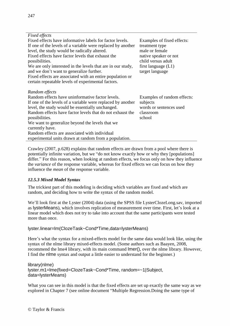
Fixed effects Fixed effects have informative labels for factor levels. Examples of fixed effects:

treatment type male or female native speaker or not child versus adult first language (L1) target language

If one of the levels of a variable were replaced by another level, the study would be radically altered. Fixed effects have factor levels that exhaust the possibilities. We are only interested in the levels that are in our study, and we don’t want to generalize further. Fixed effects are associated with an entire population or certain repeatable levels of experimental factors. Random effects Random effects have uninformative factor levels. Examples of random effects:

subjects words or sentences used classroom school

If one of the levels of a variable were replaced by another level, the study would be essentially unchanged. Random effects have factor levels that do not exhaust the possibilities. We want to generalize beyond the levels that we currently have. Random effects are associated with individual experimental units drawn at random from a population.

Crawley (2007, p.628) explains that random effects are drawn from a pool where there is potentially infinite variation, but we ―do not know exactly how or why they [populations] differ.‖ For this reason, when looking at random effects, we focus only on how they influence the variance of the response variable, whereas for fixed effects we can focus on how they influence the mean of the response variable. 12.5.3 Mixed Model Syntax

The trickiest part of this modeling is deciding which variables are fixed and which are random, and deciding how to write the syntax of the random model. We’ll look first at the Lyster (2004) data (using the SPSS file LysterClozeLong.sav, imported as lysterMeans), which involves replication of measurement over time. First, let’s look at a linear model which does not try to take into account that the same participants were tested more than once.

lyster.linear=lm(ClozeTask~Cond*Time,data=lysterMeans) Here’s what the syntax for a mixed-effects model for the same data would look like, using the syntax of the nlme library mixed-effects model. (Some authors such as Baayen, 2008, recommend the lme4 library, with its main command lmer(), over the nlme library. However, I find the nlme syntax and output a little easier to understand for the beginner.)

library(nlme) lyster.m1=lme(fixed=ClozeTask~Cond*Time, random=~1|Subject, data=lysterMeans) What you can see in this model is that the fixed effects are set up exactly the same way as we explored in Chapter 7 (see online document ―Multiple Regression.Doing the same type of

248

© Taylor & Francis

regression as SPSS‖), and we have seen this same syntax in the ANOVA tests. It is the random effects part that is new to us. Notice that the random model has two parts—the part that comes before the vertical bar and the part that comes after. The part that comes before the vertical bar will allow the slopes of the response variable to vary in accordance with the named factor, while the part that comes after the vertical bar will allow the intercepts of the response variable to vary in accordance with the named factor. If a random variable is found only after the vertical bar, as seen in the model for the Lyster data, this is called a random intercept type of mixed-effects model. The syntax random=~1|Subject means that the response variable of scores on the cloze task is allowed to vary in intercept depending upon the subject. Put another way, random intercepts mean that ―the repeated measurements for an individual vary about that individual’s own regression line which can differ in intercept but not in slope from the regression lines of other individuals‖ (Faraway, 2006, p. 164). According to Galwey (2006), one should first approach a mixed-effects model by treating as many variables as possible as fixed-effect terms. Those factors that should be treated as random effects are what Galwey (2006, p. 173) terms ―nuisance effects (block effects). All block terms should normally be regarded as random.‖ Factors you are truly interested in can be either fixed or random, depending on whether you want to generalize beyond those categories that are contained in the variable. For example, for Lyster’s data we can choose to generalize only to the time periods where data was measured, in which case we would not put this variable into the random-effects model. On the other hand, we definitely would like to generalize more widely than the particular subjects who took the test, so that term will go into the random-effects model. Another possibility for the Lyster data is the following model: lyster.m3=lme(fixed=ClozeTask~Cond*Time, random=~Time|Subject, data=lysterMeans) If there are variables on both sides of the bar, this is called the random intercepts and slope type of model. The random part of this model means that the response variable of scores on the cloze task is allowed to vary in slope depending on the time it was tested, and in intercept depending upon the particular subject being measured. Faraway (2006) says this type of model where both slopes and intercepts can vary is a more realistic model, especially for longitudinal data where observations may be highly correlated. As we will see later, this particular model for the Lyster (2004) data is not a good model, and one of the main reasons is that there are only three time periods. A time period is more appropriately put into the random effects part of the model when it is a continuous variable that is a measurement of growth. In Lyster’s study there are only three time periods, and this is thus not a continuous variable. For the Murphy data (using the murphyLong data set created in this chapter) here is one possibility for a mixed-effects model:

murphy.m1=lme(fixed=verbs~group*verbtype*similarity, random=~1|similarity/participant, data=murphyLong)

249

© Taylor & Francis

In this model the random effects are nested within each other, and this allows the intercept to vary for different participants at the level of verb similarity. The nested model is a logical model because the three terms for similarity (Distant, Intermediate, and Prototypical) are repeated for both verb types (Regular and Irregular), which means that the verb similarity category is actually nested within the verb type category, as shown in Figure 12.10. You should only put nested effects in the error term if they are replicated. Pinheiro and Bates (2000, p. 27) say ―[N]ested interaction terms can only be fit when there are replications available in the data.‖

Figure 12.10 The nested nature of the Murphy terms ―verb type‖ and ―similarity.‖ If you have effects that are nested within each other (this design is also called a split-plot design), you will need to put those nested effects in order from largest to smallest (spatially or conceptually) to the right of the vertical bar. We will note, however, that Murphy’s model is not actually a split-plot design, since all participants were asked to suffix both regular and irregular verbs. With true split-plot designs (such as the Gass and Varonis hierarchical design seen in Figure 12.9) the participants are divided by the dominating variable and then the variable that is dominated is repeated. In other words, if Murphy’s design were a split-plot design, participants would have suffixed either regular or irregular verbs only (the dominating variable), but then suffixed verbs from all of the similarity types (the dominated variable). Here is a mixed-effects model for a true split-plot design, such as the Gass and Varonis (1994) design shown earlier in the chapter: fixed=score~ScriptGroup*InteractionGroup, random=~1|ScriptGroup/InteractionGroup/ participant This idea of a mixed-effects model will surely seem new and confusing. But if you are not sure you have constructed the best model, there is no need to worry because you can try out different models and compare the fit of each model later. Checking the 95% confidence intervals of parameter estimates, both fixed and random, will also help ascertain if there are problems with the model. If parameters are extremely wide, this indicates an inappropriate model. Pinheiro and Bates say, ―Having abnormally wide intervals usually indicates problems with the model definition‖ (2000, p. 27). For more reading about syntax that is used in mixed-effects models, see Baayen (2008), Crawley (2007), Faraway (2006), Galwey (2006), and Pinheiro and Bates (2000). If you plan to use mixed-effects models regularly I do recommend further reading, as this chapter is only a short introduction. 12.5.4 Understanding the Output from a Mixed-Effects Model

You should have some idea now of how the syntax of a mixed-effects model works. Let’s examine the output we’ll receive when we summarize our created models. To contrast the output, first look at the output generated from a least squares analysis of the Lyster data.

250

© Taylor & Francis

lyster.linear=lm(ClozeTask~Cond*Time,data=lysterMeans) summary(lyster.linear)

Remember that a linear model assumes that all observations are independent. We have 540 observations, but we know that this experiment had only 180 participants. Therefore, we can see from the error degrees of freedom (528) that this model has pseudoreplication. Crawley (2007) defines pseudoreplication as analysis of the data with more degrees of freedom than you really have. Even if you don’t really understand exactly what degrees of freedom are, you need to take notice of them to make sure that your model does not show pseudoreplication. As we will see, models that correctly take the repeated measurements into account will have much lower degrees of freedom. Now let’s go ahead and run our mixed-effects model, making sure to open the appropriate library (nlme) so that the commands will work.

library(nlme) lyster.m1=lme(fixed=ClozeTask~Cond*Time, random=~1|Subject, data=lysterMeans) summary(lyster.m1)

The first line of the output describes what kind of model we have used, which is a model fit by a technique called residual maximum likelihood (REML). The next part of the output gives some measures of goodness of fit, including the Akaike information criterion (AIC),

251

© Taylor & Francis

which we have seen and used previously to compare model fit, the Bayesian information criterion (BIC), which penalizes additional parameters more heavily, and the log likelihood. These will be useful later in comparing model fits. For all of these numbers, the lower the number the better the fit, but because they are calculated differently not all of these values will always agree! Next comes information about random effects. Notice that just the standard deviation is given. There are no parameter estimates and no p-values. This is because random effects are, given the definition of the model, presumed to have a mean of zero, and it is their variance (or standard deviation, which is the square root of the variance) that we are estimating (Baayen, 2008). In a linear model, we run the model intending to estimate parameters (coefficients) of the fixed models, while in the mixed model we estimate variances of the random factors as well as parameters of the fixed factors. We have two standard deviations here, one for the effect of subject (defined relative to the intercept, so its value is found under the ―Intercept‖ column), and the other for the residuals, which is the variance the model has not been able to explain. Baayen points out that this residual variance ―is a random variable with mean zero and unknown variance, and is therefore a random effect‖ (2008, p. 268), just as our subject variable is random. For the random effects, variances (the standard deviations squared) should be reported. Crawley (2007, p. 628) says ―[v]ariance components analysis is all about estimating the size of this variance, and working out its percentage contribution to the overall variation.‖ So here we see two sources of variance—the subjects and the residual (leftover, unexplained) error. The standard deviation of the subject error is 4.39 and the residual error 3.41. Now we’ll square these to make them variances, and express each as a percentage of the total, as Crawley (2007, p. 640) explains:

sd=c(4.39, 3.41) var=sd^2 100*var/sum(var) [1] 62.36885 37.63115 This shows that the subject effect was a large 62.4% of the total variance. Only 36.6% of the variance was unexplained. I continue with the output, which shows the fixed effects of the model in regression format.

This is in the format of regression output, so, to see the ANOVA results, call for the anova() analysis of the model:

252

© Taylor & Francis

anova(lyster.m1)

In accordance with our traditional interpretation of the fixed effects, we see that both main effects and the interaction between condition and time are statistical. Continuing with the output of the model:

This part of the output is a full correlation matrix of all of the parameters. Baayen (2008) asserts that these correlations are not the same as what you would get when using the cor() command on pairs of vectors, but that these numbers ―can be used to construct confidence ellipses for pairs of fixed-effects parameters‖ (p. 268). Since we will not be doing this, Baayen suggests suppressing this part of the output by typing the following line, which then subsequently affects the summary function for the lyster.m1 model:

print(lyster.m1, corr=FALSE) Fox (2002a) concurs that the correlation output is not usually anything we would use, but does note that if there are large correlations this would be indicative of problems within the model. This is the last part of the output:

This gives quartiles of the standardized within-group residuals, and a count of the number of observations and the number of groups. Again, use this information to make sure you do not have pseudoreplication in your model. We see here that everything is in order—we did have 540 observations, but only 180 participants. Since we found a statistical interaction between condition and groups in the fixed-effects part of the model, we would want to continue to look more closely at that interaction. This could be accomplished using the pairwise.t.test() command, as explained in the online document ―Factorial ANOVA.Performing comparisons in a factorial ANOVA.‖

253

© Taylor & Francis

12.5.5 Searching for the Minimal Adequate Model

Just as was shown previously with linear models, we can look for a minimal adequate model by subtracting terms from our original model and then comparing them using anova() (note that neither step() nor boot.stepAIC() is available for a mixed-effects model). In this case, though, we cannot compare mixed-effects models with different fixed-effect terms if we are using the REML method. We must switch to the normal maximum likelihood method by specifying method="ML" in our model. On the other hand, if you want to compare differences in the random effects part of the model, you do not need to switch methods. To make this process clearer, let’s look again at the Lyster data. In the ANOVA output, the interaction of condition and time was statistical, leading us to believe we cannot simplify this model any further (remember, if the interaction is statistical then we must keep the component main effects of the interaction). However, just to illustrate the fact that we need to keep the interaction, we can subtract the interaction out of the model and compare models using the log likelihood test. Because we are changing the fixed part of the model, we must change to the ―ML‖ method: lyster.m1=lme(fixed=ClozeTask~Cond*Time, random=~1|Subject, data=lysterMeans, method="ML")

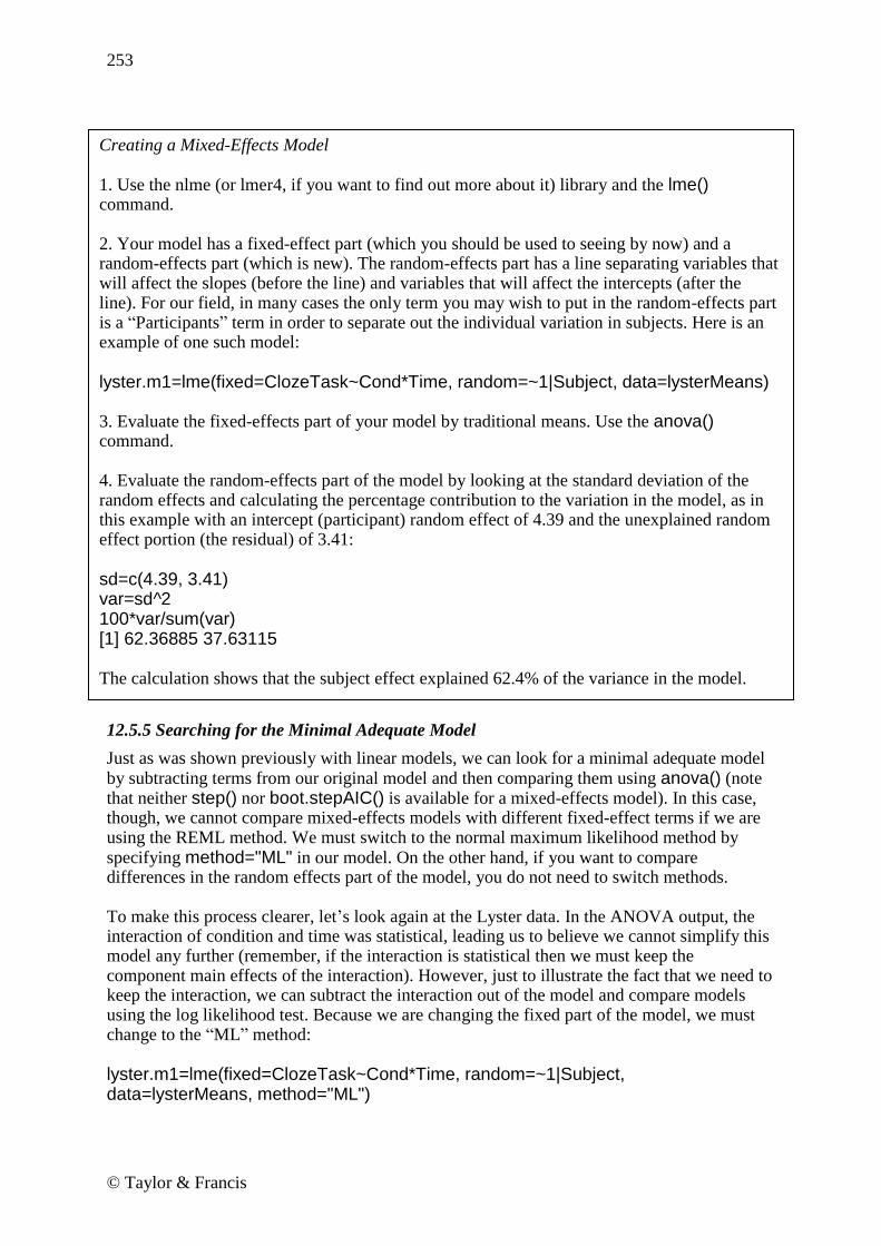
Creating a Mixed-Effects Model 1. Use the nlme (or lmer4, if you want to find out more about it) library and the lme() command. 2. Your model has a fixed-effect part (which you should be used to seeing by now) and a random-effects part (which is new). The random-effects part has a line separating variables that will affect the slopes (before the line) and variables that will affect the intercepts (after the line). For our field, in many cases the only term you may wish to put in the random-effects part is a ―Participants‖ term in order to separate out the individual variation in subjects. Here is an example of one such model:

lyster.m1=lme(fixed=ClozeTask~Cond*Time, random=~1|Subject, data=lysterMeans) 3. Evaluate the fixed-effects part of your model by traditional means. Use the anova() command. 4. Evaluate the random-effects part of the model by looking at the standard deviation of the random effects and calculating the percentage contribution to the variation in the model, as in this example with an intercept (participant) random effect of 4.39 and the unexplained random effect portion (the residual) of 3.41:

sd=c(4.39, 3.41) var=sd^2 100*var/sum(var) [1] 62.36885 37.63115 The calculation shows that the subject effect explained 62.4% of the variance in the model.

254

© Taylor & Francis

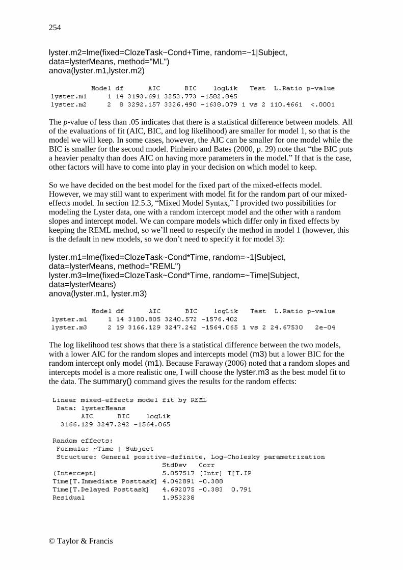
lyster.m2=lme(fixed=ClozeTask~Cond+Time, random=~1|Subject, data=lysterMeans, method="ML") anova(lyster.m1,lyster.m2)

The p-value of less than .05 indicates that there is a statistical difference between models. All of the evaluations of fit (AIC, BIC, and log likelihood) are smaller for model 1, so that is the model we will keep. In some cases, however, the AIC can be smaller for one model while the BIC is smaller for the second model. Pinheiro and Bates (2000, p. 29) note that ―the BIC puts a heavier penalty than does AIC on having more parameters in the model.‖ If that is the case, other factors will have to come into play in your decision on which model to keep. So we have decided on the best model for the fixed part of the mixed-effects model. However, we may still want to experiment with model fit for the random part of our mixed-effects model. In section 12.5.3, ―Mixed Model Syntax,‖ I provided two possibilities for modeling the Lyster data, one with a random intercept model and the other with a random slopes and intercept model. We can compare models which differ only in fixed effects by keeping the REML method, so we’ll need to respecify the method in model 1 (however, this is the default in new models, so we don’t need to specify it for model 3):

lyster.m1=lme(fixed=ClozeTask~Cond*Time, random=~1|Subject, data=lysterMeans, method="REML") lyster.m3=lme(fixed=ClozeTask~Cond*Time, random=~Time|Subject, data=lysterMeans) anova(lyster.m1, lyster.m3)

The log likelihood test shows that there is a statistical difference between the two models, with a lower AIC for the random slopes and intercepts model (m3) but a lower BIC for the random intercept only model (m1). Because Faraway (2006) noted that a random slopes and intercepts model is a more realistic one, I will choose the lyster.m3 as the best model fit to the data. The summary() command gives the results for the random effects:

255

© Taylor & Francis

We want to estimate how much each factor adds to the variance, so use the formula found in the summary box for ―Creating a Mixed-Effects Model‖ at the end of section 12.5.4, adding in all four of the variances that we have (note that the intercept variance represents the variance for the pre-test, because it is the default level of the variable):

sd=c(5.06, 4.04, 4.69, 1.95) var=sd^2 100*var/sum(var) [1] 37.805912 24.100242 32.479128 5.614717 This result shows that the pre-test accounted for 37.8% of the variance, the immediate post-test 24.1%, the delayed post-test 32.5%, and there was only 5.6% of the variance that was not accounted for which ends up as error. For the fixed effects Pinheiro and Bates (2000) say we should examine the results with the anova() command and not by examining the t-values and p-values of the regression output. With the different model the ANOVA evaluation has different F-values than the first model, but the conclusion that all main effects and interactions in the model are statistical does not change:

anova(lyster.m3)

We can use the command in lme called intervals() to call for 95% confidence intervals of all the parameters.

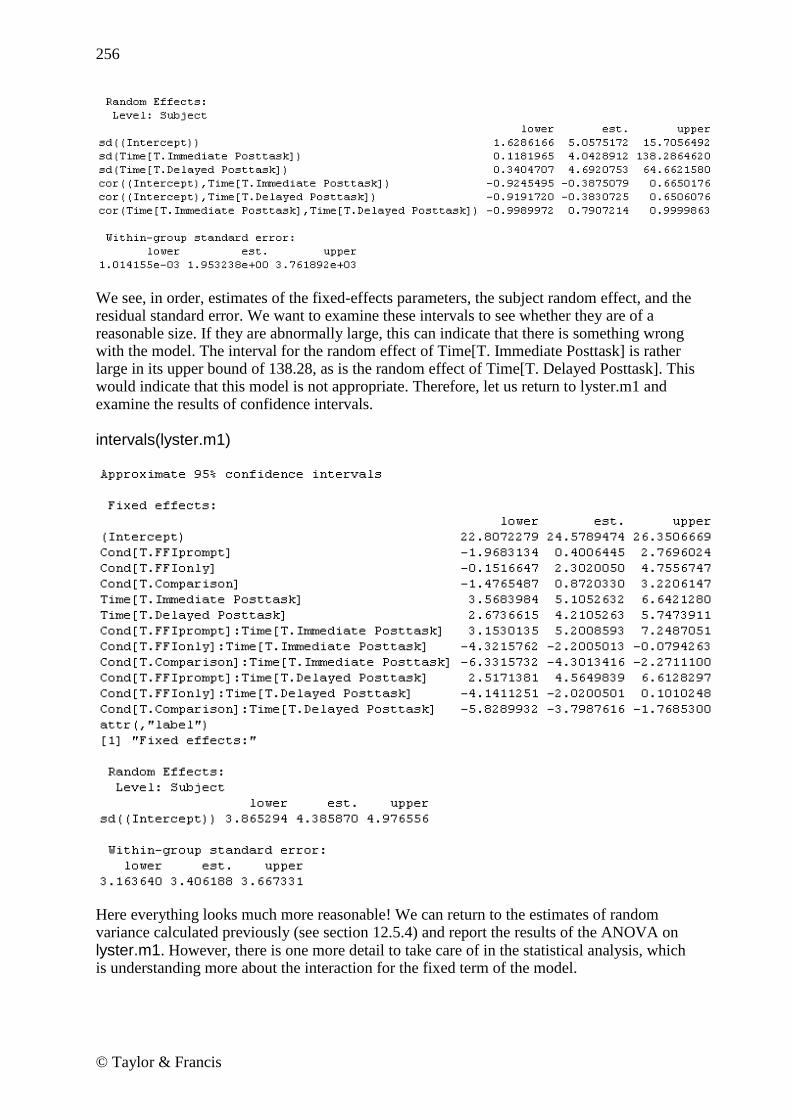
intervals(lyster.m3)

256

© Taylor & Francis

We see, in order, estimates of the fixed-effects parameters, the subject random effect, and the residual standard error. We want to examine these intervals to see whether they are of a reasonable size. If they are abnormally large, this can indicate that there is something wrong with the model. The interval for the random effect of Time[T. Immediate Posttask] is rather large in its upper bound of 138.28, as is the random effect of Time[T. Delayed Posttask]. This would indicate that this model is not appropriate. Therefore, let us return to lyster.m1 and examine the results of confidence intervals.

intervals(lyster.m1)

Here everything looks much more reasonable! We can return to the estimates of random variance calculated previously (see section 12.5.4) and report the results of the ANOVA on lyster.m1. However, there is one more detail to take care of in the statistical analysis, which is understanding more about the interaction for the fixed term of the model.

257

© Taylor & Francis

In looking at the Lyster (2004) research design, it is clear that all of the subjects who were not in the comparison group improved their scores in the post-tests. What we are therefore particularly interested in knowing is which group performed the best at the first and second post-tests. I recommend following Howell’s (2002) advice for RM ANOVA, which is to run separate ANOVAs at each level of one factor. To address these issues, let’s model two ANOVAs at each of the post-test times. First we must subset the data to contain only the immediate post-test scores; then we can model the ANOVA and run multiple comparisons using the glht() command (find out more information about this command in the online document ―One way ANOVA.One-way ANOVA test‖).

lyster.post1=subset(lysterMeans,subset=Time=="Immediate Posttask") post1.m1=lm(ClozeTask~Cond,data=lyster.post1) library(multcomp) post1.pairs=glht(post1.m1,linfct=mcp(Cond="Tukey")) confint(post1.pairs)

For the first post-test, 95% confidence intervals show differences between all groups except FFI only versus FFI recast. Recalling the mean scores of the conditions on the cloze test: numSummary(lyster.post1[,"ClozeTask "],groups=lyster.post1$Cond)

We can say that FFI prompt scored statistically better than any other group, the comparison group scored statistically lowest, and FFI recast and FFI were in the middle but not statistically different from one another. Written another way, this could be expressed by: FFI prompt > FFI recast, FFI only > Comparison Redoing this process for the second post-test, results are almost identical, but now the FFI recast group is not statistically different from the comparison group either, meaning that the FFI prompt group is statistically better than all other groups, FFI only is statistically better than the comparison group, and FFI recast and comparison are not different from one another. Note that we have run a couple more tests than just the mixed-effects model, but we really don’t need to worry that there is anything wrong with this, according to Howell (2002). The only caveats that Howell provides are that you do not need to include every result which you obtain, and that if you do run a significant number of additional tests then you ought to think about adjusting the p-values to stay within the familywise error rate. Only those results which are relevant to your hypotheses need to be reported, and you can ignore the rest, and in this

258

© Taylor & Francis

case we did not run a large number of additional tests, so we won’t worry about adjusting p-values. 12.5.6 Testing the Assumptions of the Model

Just as with any type of regression modeling, we need to examine the assumptions behind our model after we have settled on the minimal adequate model. The assumptions of a mixed-effects model are somewhat different than those we are used to seeing for parametric statistics. Crawley (2007, p. 628) says there are five assumptions:

1. ―Within-group errors are independent with mean zero and variance σ2.‖ 2. ―Within-group errors are independent of the random effects.‖ 3. ―The random effects are normally distributed with mean zero and covariance matrix

Ψ.‖ 4. ―The random effects are independent in different groups.‖ 5. ―The covariance matrix does not depend on the group.‖

The plot command is the primary way of examining the first two assumptions that concern the error component. The first plot is a plot of the standardized residuals versus fitted values for both groups:

plot(lyster.m1, main="Lyster (2004) data")

Figure 12.11 Fitted values vs. standardized residual plots to examine homoscedasticity assumptions for Lyster (2004). The plot in Figure 12.11 is used to assess the assumption of the constant variance of the residuals. Remember that these plots should show a random scattering of data with no tendency toward a pie shape. This residual plot indicates some problems with heteroscedasticity in the residuals because there is a tapering of the data on the right-hand side of the graph. We can study these plots further by examining them by group as shown in Figure 12.12.

Lyster (2004) data

Fitted values

Sta

nd

ard

ize

d r

esid

ua

ls

-2

-1

0

1

2

3

15 20 25 30 35 40

259

© Taylor & Francis

plot(lyster.m1,resid(.,type="p")~fitted(.)|Cond)

Figure 12.12 Fitted values vs. standardized residual plots divided by groups in Lyster (2004). For the Lyster (2004) data, it appears that it is group 2 (FFI+prompt) where the data are heteroscedastic, since it is the lower right-hand corner box that shows the real tapering off of values on the right-hand side of the graph. It is possible to fit variance functions in lme that will model heteroscedasticity (and thus correct for it), but this topic is beyond the scope of this book (see Pinheiro and Bates, 2000, Chapter 5 for more information). The following command looks for linearity in the response variable by plotting it against the fitted values (the with command lets me specify the data set for each command):

with(lysterMeans, plot(lyster.m1,ClozeTask~fitted(.)))

Fitted values

Sta

nd

ard

ize

d r

esid

ua

ls

-2

-1

0

1

2

3

15 20 25 30 35 40

FFIrecast FFIprompt

FFIonly

15 20 25 30 35 40

-2

-1

0

1

2

3

Comparison

260

© Taylor & Francis

Figure 12.13 Response variable plotted against fitted values to examine linearity assumption for Lyster (2004) data. The plot returned by this command in Figure 12.13 looks reasonably linear. Next we can examine the assumption of normality for the within-group errors (assumption 3) by looking at Q-Q plots. Notice that this command calls for Q-Q plots that are divided into different categories of time for the Lyster (2004) data. qqnorm(lyster.m1,~resid(.)|Time)

Figure 12.14 Q-Q plots to examine normality assumption for Lyster (2004) data.

Fitted values

Clo

ze

Ta

sk

10

15

20

25

30

35

40

15 20 25 30 35 40

Residuals

Qu

an

tile

s o

f sta

nd

ard

no

rma

l

-2

0

2

-5 0 5 10

Pretask Immediate Posttask

-2

0

2

Delayed Posttask

261

© Taylor & Francis

Figure 12.14 does not seem to show any departures from normality. We could examine Q-Q plots for other divisions of the data, such as the interaction of Time and Condition:

qqnorm(lyster.m1,~resid(.)|Time:Cond) Everything still looks very normal. In sum, just as with many of our real data sets, these data do not appear to satisfy all of the assumptions of our model. For assumptions about random effects (assumption 4) we will look at a Q-Q plot of the random effects. The estimated best linear unbiased predictors (BLUPs) of the random effects can be extracted with the ranef command:

qqnorm(lyster.m1,~ranef(.)) This graph shows that the assumption of normality is reasonable (it is not shown here). For help in checking the fifth assumption listed here, that of the homogeneity of the random effects covariance matrix, see Pinheiro and Bates (2000). 12.5.7 Reporting the Results of a Mixed-Effects Model

When reporting the results of a mixed-effects model, you should give the reader your minimal adequate model, and state whether you considered other models in your search for the best model. If several models were considered, then the AIC for each model should be reported. The best model for the data should be reported with the appropriate fixed-effect parameters. For the random effects, variances (the standard deviations squared) should be reported and the percentage variance that the random effects explain can be noted. An ANOVA summary of the model will generally be most appropriate for telling your reader about statistical terms in the model if that is your interest. Although you could construct a regression equation with the fixed-effect parameters, I don’t think most people who are doing repeated-measures analyses are looking for regression models. They are looking to see whether there are group differences, and these are best addressed by ANOVA summaries and then further analysis with multiple comparisons to see which factor levels differ statistically from each other, and what their confidence intervals and effect sizes are. Here is a sample report about a mixed-effects model of the Lyster data with the cloze task: The minimal adequate model for the cloze task in Lyster (2004) is:

fixed=ClozeTask~Cond + Time + Cond:Time, random=~1|Subject In the fixed-effects part of the model, the main effect of Condition was statistical (F3,176=11.2, p<.0001, partial eta-squared=.16), the main effect of Time was statistical (F2,352=100.8, p<.0001, partial eta-squared=.36), and the interaction of Condition and Time was statistical (F6,352=21.1, p<.0001, partial eta-squared=.26). Further examination of the interaction between Condition and Time showed that, for the immediate post-test, the FFI prompt group performed statistically better than all other groups, while the FFI recast and FFI only groups performed statistically better only than the comparison group. For the delayed post-test, the FFI prompt group performed statistically better than all other groups, the FFI only group was

262

© Taylor & Francis

statistically better than the comparison group, and there was no statistical difference between the FFI recast and comparison groups. It is clear that recasting by using prompts produced the best results for this task. In the random effects part of the model the intercept of participants was allowed to vary. Another model where both slopes and intercepts were allowed to vary was tested (random=time|Subject) and had an AIC of 3166 (as compared to 3180 for the model shown above), but confidence intervals for this model were too wide, showing problems with the model, so it was rejected. The standard deviation was 4.39 for the subject effect and 3.41 for the error, meaning that the effect of subjects accounted for 62.4% of the total variance. Examination of model assumptions showed heteroscedasticity in the data. 12.6 Application Activities for Mixed-Effects Models

1. Using the mixed-effects model proposed in section 12.5.1 (right before Figure 12.9), find the best way to model the variable of verbs in the Murphy data set (be sure to open the nlme library first; also, import the SPSS file MurphyLongForm.sav as murphyLong for this exercise; look at the structure of the data and make sure group, verbtype, and similarity are factors—if you don’t have the correct structure, you will get an error message with something about ―Error in MEEM‖). Look at the fixed effects—will you keep the full factorial model or reduce it? Compare the syntax of the random model found in the online document (one with ―similarity‖ and ―participant‖ in the random model) to a random model with only the one term of ―participant.‖ Examine model assumptions. 2. Write a mixed-effects model for following research designs (start with the maximal model for the fixed effects). There is no right answer for the random effects part, but in most cases you will want to let intercepts vary by participant. a. Toth (2006): 3 (group: type of input) × 3 (time tested) RM ANOVA, repeated measures on the time of testing. b. Erdener and Burnham (2005): 4 (condition of orthographic and audio-visual material) × 2 (L1) × 2 (L2) RM ANOVA, repeated measures on the condition. c. Larson-Hall (2004): 16 (contrast) × 3 (proficiency level) RM ANOVA, repeated measures on the contrast. 3. Lyster (2004) binary-choice test. Import the Lyster.Written.sav file as lyster. In order to conduct this test you will need to rearrange the data into the long form, with the columns for PreBinary, Post1Binary, and Post2Binary all in one column. Next construct a mixed-effects model and use the results of anova() to report on statistical terms. Report on the variances for the random effects, and calculate percentages for variances. Describe your search for the minimal adequate model. Try to fit at least one other model and perform a log-likelihood test with anova. Perform additional tests to answer the question of which groups were statistically better at the immediate post-test. Perform checks on model assumptions and report on how well the data fit the assumptions.