An algorithm for panel ANOVA with grouped data

Metrika (2011) 74:85–107DOI 10.1007/s00184-009-0291-y

An algorithm for panel ANOVA with grouped data

Carmen Anido · Carlos Rivero · Teofilo Valdes

Received: 1 November 2008 / Published online: 7 November 2009© Springer-Verlag 2009

Abstract In this paper, we present an algorithm suitable for analysing the varianceof panel data when some observations are either given in grouped form or are missed.The analysis is carried out from the perspective of ANOVA panel data models withgeneral errors. The classification intervals of the grouped observations may vary fromone to another, thus the missing observations are in fact a particular case of grouping.The proposed Algorithm (1) estimates the parameters of the panel data models; (2)evaluates the covariance matrices of the asymptotic distribution of the time-dependentparameters assuming that the number of time periods, T , is fixed and the numberof individuals, N , tends to infinity and similarly, of the individual parameters whenT → ∞ and N is fixed; and, finally, (3) uses these asymptotic covariance matrixestimations to analyse the variance of the panel data.

Keywords Panel data · Iterative estimation · ANOVA with grouped data ·Conditional imputation · Asymptotics

C. AnidoDepartamento de Análisis Económico: Economía Cuantitativa,Facultad de Ciencias Económicas y Empresariales,Universidad Autónoma de Madrid, Cantoblanco, 28049 Madrid, Spain

C. RiveroDepartamento de Estadística e I.O. II, Facultad de Ciencias Económicas y Empresariales,Universidad Complutense de Madrid, 28223 Pozuelo de Alarcón, Spain

T. Valdes (B)Departamento de Estadística e I.O. I, Facultad de Matemáticas,Universidad Complutense de Madrid, 28040 Madrid, Spaine-mail: [email protected]

123

86 C. Anido et al.

1 Problem presentation and paper design

The algorithm presented in this paper focuses on the analysis of variance panel datamodel yit = μ+ αi + βt + ηi t , (i = 1, . . . , N , t = 1, . . . , T ). The sub-indexes i andt represent individuals and time periods, respectively, yit denotes the data of the indi-vidual i at time t , and the η′i t s are random errors. The remaining terms are parameterswith the usual constraints α1+· · ·+αN = 0 and β1+· · ·+βT = 0, which ensure themodel is identifiable. Our intention is to test for constant effects (either over the indi-viduals or over time) when the two following assumptions are made: (a) some of thevalues yit are given in grouped form (meaning that their exact values are lost, althoughwe know their grouping intervals which may vary from one data to another) or aremissed (a special case of grouped data with a unique classification interval equal to thewhole line); and (b) the distribution of the errors is general, not necessarily normal.The usual statistical methods become inapplicable under the assumptions made. Asan example, let us suppose that we aim to test that the time effects are constant (i.e.,β1 = · · · = βT ), since a similar rationale is applicable to test for constant individualeffects. The test implicitly means that T is fixed, thus, if we intend to use the asymp-totic distribution of the parameters to carry out the test, only N must tend to infinity.However, as N increases, the number of parameters of the model also increases bythe same order as N , due to the existence of individual-terms. Thus, the search forthe asymptotic distribution, as N →∞, of all the parameters of the model becomespointless. In spite of this, the search for the asymptotic distribution of the time-depen-dent parameters is pertinent, as its dimension is assumed to be fixed. Although severaltransformations of the aforementioned model (see Hsiao 2003 or Baltagi 1995) mayeliminate the individual-terms (e.g., through yit − yi. = βt + (ηi t − ηi.) or similarmodels, which could be estimated by generalized least squares in the case of normalerrors), the existence of grouped data may result in the majority of the values yit − yi.

becoming grouped, which has a pernicious, occasionally pathologic, effect as the infor-mation lost may be complete. For example, if one single value yit (t = 1, . . . , T ) ismissed, then all yit − yi. (i = 1, . . . , N ) are also missed. Therefore the transformationcited above becomes inapplicable. Additionally, the transformed model errors ηi t− ηi.

are dependent, and their distribution may be difficult to determine if the independenterrors ηi t are not normal. These comments show the kind of distortions that derivefrom the assumptions made.

Assuming the existence of grouped data, the algorithm that we propose in thispaper is valid to estimate the time (individual)-dependent parameters of model (1),and also to test for constant time (individual) effects in this model from the asymptoticdistribution of these parameters as N → ∞ (T → ∞). Assuming that N and T arefixed, the estimation of the N + T − 1 independent parameters of model (1) from theNT observations may be tackled through the EM algorithm (see Dempster et al. 1977;Little and Rubin 1987; Tanner 1993; McLachlan and Krishnan 1997; Lange 1999, forinstance), for which, as known, there exist several antecedents (e.g., the missing infor-mation principle of Orchard and Woodbury (1972), and the algorithm of Healy andWestmacott (1956) when the errors follow a normal distribution). The rationale thatjustifies our proposal will be explained in detail later. For the moment, it is sufficientto make the following general observations as a mere presentation of the origin and

123

An algorithm for panel ANOVA with grouped data 87

general structure of our algorithm, as well as of its advantages compared to the EM,its natural competitor:

(a) The idea that motivated our proposal was the EM algorithm applied to the initialpanel model with grouped data and normal errors; in spite of this, our algorithmis applicable for a wide class of error distributions, namely, the strongly unimodaldistributions, which include the normal distribution among many others.

(b) The proposed algorithm consists of two phases. Firstly, it starts estimating allof the parameters of model (1) for the finite number of observations available(N and T fixed). For this the algorithm uses the information provided by boththe precise and grouped data. Secondly, the ANOVA analysis is carried out,which will be based in asymtotics. For example, testing for constant time effects(β1 = · · · = βT ) is accomplished through the estimation (from the NT avail-able observations) of the asymptotic covariance matrix of the time parameterestimates, as N → ∞ and with T fixed. The individual parameters, αi , needto be dropped out of the aforementioned asymptotics, otherwise, the asymptoticcovariance would be infinite dimensional, thus impossible to estimate from afinite number of data. These two phases also need to be completed if the ANOVAanalysis is carried out by means of the EM algorithm. However, the EM typicallyrefers only to the parameter estimating process, therefore, in addition to this,one has to evaluate the Fisher information matrix through any of the numericalprocedures that have been proposed in this respect within the context of the EM.

(c) With normal errors, the estimating part of our algorithm agrees with its naturalestimating competitor, the EM algorithm, in presence of grouped data. Thus, ourestimates and the maximum likelihood estimates coincide in this case. However,with non-normal errors the estimating stage of our algorithm differs from theEMs. In this case, our estimating process has a clear computational advantagecompared to the EM, since the maximization step (M) of the EM usually requiresa numerical implementation which is substituted with ordinary least square pro-jections in our algorithm.

(d) Finally, with either normal or non-normal errors our estimation procedure ofthe asymptotic covariance matrices of the time (individual) parameter estimates,completely differs from, and is simpler than, the numerical methods which havebeen proposed within the context of the EM to estimate the Fisher informa-tion matrix. These later methods essentially tackle the estimation of the secondderivatives of the log-likelihood function by direct computational/numerical dif-ferentiation (Meilijson 1989), the Louis’ (1982) method or using IM iterates(Meng and Rubin 1991 ). All of them are numerical and quite unstable. Onthe contrary we will see in Sects. 2 and 3 that the equivalent estimation in ouralgorithm is simpler, since only first derivatives in analytical form are involved.

The paper is organized as follows. In Sect. 2 we describe the insides of our algorithm.Section 3 is dedicated to the hypotheses testing procedure. Its performance is con-sidered in Sects. 4 and 5. Firstly, a large amount of computer simulations are shownand commented on. Secondly, some case studies are considered. Section 6 brings thepaper to a close after commenting on some final remarks.

123

88 C. Anido et al.

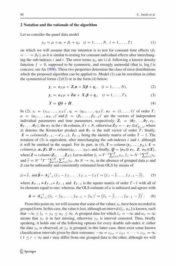
2 Notation and the rationale of the algorithm

Let us consider the panel data model

yit = μ+ αi + βt + ηi t (i = 1, . . . , N , t = 1, . . . , T ) (1)

on which we will assume that our intention is to test for constant time effects (β1= · · · = βT ), as it is similar to testing for constant individual effects after interchang-ing the sub-indexes i and t . The error terms ηi t are i.i.d. following a known densityfunction f > 0, supposed to be symmetric, and strongly unimodal (that is, log f isconcave; see An 1998). These two properties determine the class of error distributionswhich the proposed algorithm can be applied to. Model (1) can be rewritten in eitherthe symmetrical forms (2)/(3) or in the form (4) below:

yi = eT μ+ Ziα + Xβ + ηi , (i = 1, . . . , N ), (2)

yt = eN μ+ Zα + Xtβ + ηt , (t = 1, . . . , T ), (3)

Y = Qδ + H . (4)

In (2), yi = (yi1, . . . , yiT )′ , ηi = (ηi1, . . . , ηiT )′, eT = (1, . . . , 1)′ of order T ;α = (α1, . . . , αN−1)

′ and β = (β1, . . . , βT−1)′ are the vectors of independent

individual parameters and time parameters, respectively; Zi = (0T , . . .,0T , eT ,

0T , . . .,0T ), the eT in the i-th column, if i < N , otherwise ZN =− eT ⊗ e′N−1, where⊗ denotes the Kronecker product and 0T is the null vector of order T ; finally,X = column(IT−1,− e′T−1), IT−1 being the identity matrix of order T − 1. The

notation of (3) is equivalent, after interchanging the sub-indexes i and t , althoughit will be omitted in the sequel. For its part, in (4), Y= column (y1, . . ., yN ), δ =column(μ,α, β), H= column(η1, . . . , ηN ), and, finally, Q = (

eN⊗ eT, Z, eN⊗X),

where Z= column (Z1, . . ., ZN ). Let us define yi.= T−1∑Tt=1 yit , y.t = N−1∑N

i=1 yit

and ¯y = N−1T−1∑Ni=1

∑Tt=1 yit . As N →∞, in the absence of grouped data μ and

β can be unbiasedly and consistently estimated from OLS by means of

μ= ¯y, and β= A−1T−1 (y.1 − y.T , . . . , y.T−1 − y.T )′ = (

y.1 − ¯y, . . . , y.T−1 − ¯y), (5)

where AT−1 = IT−1+ 1T−1 and 1T−1 is the square matrix of order T−1 with all ofits elements equal to one; whereas, the OLS estimate of α is unbiased and agrees with

α = A−1N−1 (y1. − yN ., . . . , yN−1. − yN .)

′ = (y1. − ¯y, . . . , yN−1. − ¯y

)′. (6)

From this point on, we will assume that some of the values yit have been recorded ingrouped form. In this case, the value is lost, although an interval (li t , uit ] is known, suchthat −∞ ≤ li t < yit ≤ uit ≤ ∞. A grouped data for which li t = −∞ and uit = ∞means that yit is in fact missing, otherwise yit is interval censored. Thus, brieflyspeaking, it holds one of the following options for every double sub-index it: eitherthe data yit is observed, or yit is grouped; in this latter case, there exist some knownclassification intervals given by their extremes:−∞ = cito < cit1 < · · · < citr = ∞( 1 ≤ r < ∞ and r may differ from one grouped data to the other, although we will

123


omit this possible dependency). The interval (li t , uit ] corresponding to the groupeddata yit agrees with one of the classification intervals (cits, cits+1] mentioned above.

The existence of grouped data makes the use of the estimates (5) and (6) imprac-ticable. Assuming that the number of individuals and the number of time periods arefixed, let us partition the set of sub-indexes I = {i t |i = 1, . . ., N , t = 1, . . ., T } inthe following two sets: Io = {i t |yit is observed, i = 1, . . ., N , t = 1, . . ., T } andIg= I\I o = {i t |yit is grouped, i = 1, . . ., N, t = 1, . . ., T}. We propose to estimatethe true vector parameter δ by means of an iterative algorithm based on OLS estimatesand conditional imputations given the current value assigned to δ. It will be shown thatthe algorithm converges, independent of the initial value chosen. The limit point of thealgorithm will define our estimate of δ. Then, our intention being to test for constanttime effects, the focus will be on the asymptotic distribution of the β-estimates whenN tends to infinity. This distribution will allow us to test for constant time-dependentparameters as well as other linear transformations of β. A similar procedure can beused to test for constant individual effects. In this case, we need to assume N to beconstant and T → ∞ in the search of the asymptotic distribution of the individual-dependent parameters. Strictly speaking, assuming N and T to be fixed, the proposedalgorithm, to estimate δ, runs as follows:

123

90 C. Anido et al.

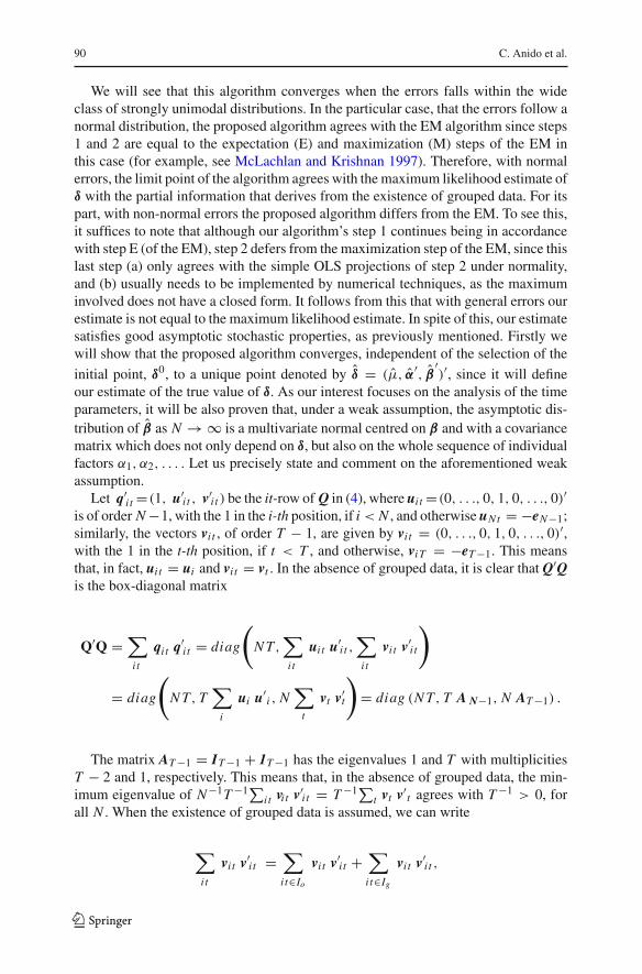
We will see that this algorithm converges when the errors falls within the wideclass of strongly unimodal distributions. In the particular case, that the errors follow anormal distribution, the proposed algorithm agrees with the EM algorithm since steps1 and 2 are equal to the expectation (E) and maximization (M) steps of the EM inthis case (for example, see McLachlan and Krishnan 1997). Therefore, with normalerrors, the limit point of the algorithm agrees with the maximum likelihood estimate ofδ with the partial information that derives from the existence of grouped data. For itspart, with non-normal errors the proposed algorithm differs from the EM. To see this,it suffices to note that although our algorithm’s step 1 continues being in accordancewith step E (of the EM), step 2 defers from the maximization step of the EM, since thislast step (a) only agrees with the simple OLS projections of step 2 under normality,and (b) usually needs to be implemented by numerical techniques, as the maximuminvolved does not have a closed form. It follows from this that with general errors ourestimate is not equal to the maximum likelihood estimate. In spite of this, our estimatesatisfies good asymptotic stochastic properties, as previously mentioned. Firstly wewill show that the proposed algorithm converges, independent of the selection of the

initial point, δ0, to a unique point denoted by δ = (μ, α′, β′)′, since it will define

our estimate of the true value of δ. As our interest focuses on the analysis of the timeparameters, it will be also proven that, under a weak assumption, the asymptotic dis-tribution of β as N →∞ is a multivariate normal centred on β and with a covariancematrix which does not only depend on δ, but also on the whole sequence of individualfactors α1, α2, . . . . Let us precisely state and comment on the aforementioned weakassumption.

Let q′i t=(1, u′i t , v′i t ) be the it-row of Q in (4), where ui t=(0, . . ., 0, 1, 0, . . ., 0)′is of order N−1, with the 1 in the i-th position, if i < N , and otherwise uNt = −eN−1;similarly, the vectors vi t , of order T − 1, are given by vi t = (0, . . ., 0, 1, 0, . . ., 0)′,with the 1 in the t-th position, if t < T , and otherwise, viT = −eT−1. This meansthat, in fact, ui t = ui and vi t = vt . In the absence of grouped data, it is clear that Q′Qis the box-diagonal matrix

Q′Q =∑

i t

qi t q′i t = diag

(

N T,∑

i t

ui t u′i t ,∑

i t

vi t v′i t

)

= diag

(

N T, T∑

i

ui u′i , N∑

t

vt v′t

)

= diag (N T, T A N−1, N AT−1) .

The matrix AT−1 = IT−1 + 1T−1 has the eigenvalues 1 and T with multiplicitiesT − 2 and 1, respectively. This means that, in the absence of grouped data, the min-imum eigenvalue of N−1T−1∑

i t vi t v′i t = T−1∑t vt v′t agrees with T−1 > 0, for

all N . When the existence of grouped data is assumed, we can write

∑

i t

vi t v′i t =∑

i t∈Io

vi t v′i t +∑

i t∈Ig

vi t v′i t ,

123


where the use of double sub-indexes in the terms of the sum becomes unavoidable. Theweak assumption that was mentioned is similar to that seen in the absence of groupeddata: the minimum eigenvalues of the matrices N−1T−1 ∑

i t∈Iovi t v′i t are bounded

from below by a positive value. The following assumption strictly establishes this, andit will be assumed in the sequel when we test for constant time effects.

Weak assumption (on time coefficients)

Assuming T to be fixed,

ξN > ξ > 0 (11)

f orall N , whereξN istheminimumeigenvalueof thematri x N−1T−1 ∑i t∈Io

vi t v′i t .Assumption (11) may be weakened by imposing ξN > ξ > 0, for all N ≥ M .

Also, if the data grouping mechanism is random, it is sufficient that this assumptionbe fulfilled almost everywhere (a.e.). The reader can verify this from the proofs ofTheorem 1. Although Assumption (11) does not permit, for instance, that all of theobservations can be grouped, some examples in which this assumption is satisfied areshown below:

Example 1 Let us suppose that each data yit independently has probabilities p > 0and 1− p of being observed and of being given in grouped form, respectively. For afixed number of individuals, N , let us denote by Nt = #{i t |yit ∈ Io}. It is clear that,as N →∞, N−1 Nt → p a.e., and

N−1T−1∑

i t∈Io

vi t v′i t = N−1T−1 (diag (N1, . . . , NT−1)

+NT 1T−1) →N→∞ pT−1 AT−1 a.e..

Therefore, ξN → pT−1 > 0 a.e. and the basic hypothesis holds in the weakenedform mentioned above.

Example 2 As before, if the values yit (t = 1, . . ., T ) of the individual i have probabil-ities pi > 0 and 1− pi of being observed or being given in grouped form, respectivelyand additionally, we assume that

N−1N∑

i=1

pi →N→∞ p > 0 a.e., (12)

then N−1 Nt → p a.e. and ξN → pT−1 > 0, a.e. as in case 1. The convergence (12)holds, for example, if p1, . . ., pN are i.i.d. from a distribution (e.g., uniform, beta,etc.) on the interval (0, 1) with mean p.

The following two theorems formally state: (a) the convergence of the proposed esti-mating algorithm, assuming that N and T are fixed; (b) the asymptotic normality of

123

92 C. Anido et al.

the distributions of μ− μ and β − β; and (c) the consistent estimation of the covari-ance matrices of the asymptotic distributions specified in the former point (b). In thenext section, these results will be taken into account to test for constant effects or, ingeneral, other linear transformations of the time or individual dependent parametersof model (1).

Theorem 1 If the error distribution is strongly unimodal, then

(i) Assuming that N and T are fixed, the sequence {δ p = (μp,α p,β p)′} gen-erated by the proposed algorithm converges, as p → ∞, to a unique point,

δ = (μ, α′, β′)′, for any initial point δ0 = (μ0,α0,β0)′.

In addition, if assumption (11) holds, then

(ii) (Time-dependent factor part: T fixed) As N → ∞, β and μ areconsistent estimates of the true parameters β and μ , respectively. Let

L(√

N T(β − β

))and L

(√N T

(μ− μ

))denote the distribution laws

of√

N T(β − β

)and√

N T(μ− μ

), respectively. It holds that, as N→∞,

L(√

N T(β − β

))and L

(√N T

(μ− μ

))weakly converge to some nor-

mal distributions, N (0,Λ(μ,β,α∞)) and N (0, σ (μ,β,α∞)), respectively,for some non-null covariance matrix Λ(μ,β,α∞) and some σ(μ,β,α∞)

> 0. Both Λ(μ,β,α∞) and σ(μ,β,α∞) do not only depend on the true

δ = (μ, α′, β′)′, which was defined for fixed values of N and T, but also on

the whole sequence of individual factors α∞ = (α1, α2, . . .).

Proof (i) For any real values a < b, let us define the non-decreasing function γab(z)given by the conditional expectation

γab (z) = E(η|a + z < η ≤ b + z),

where η denotes any error ηi t .Firstly, let us start by proving that z − γab(z) is also non-decreasing as a function

of z. It is clear that (1) γab(z + d) = γa+d,b+d(z) and (2) given b > 0, γ−b,b(z) is anodd function of z; thus, it is sufficient to prove that z−γ−b,b(z) does not decrease overz > 0, for any fixed value b > 0. It can easily be verified that this occurs if and onlyif the ratio f (t)/ f (t + τ ) is non-decreasing as a function of t , for any given τ >0.Finally, this last assertion holds if f is strongly unimodal, as assumed. To see this, letus note that, if log f is concave then, for τ > 0 and c > 0,

− f (t + c + τ)− f (t + c)

τ f (t + c)≥ − f (t + τ)− f (t)

τ f (t),

hence

f (t + c)

f (t + c + τ)≥ f (t)

f (t + τ).

123


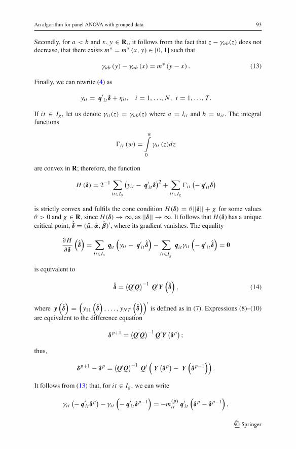
Secondly, for a < b and x, y ∈ R,, it follows from the fact that z − γab(z) does notdecrease, that there exists m∗ = m∗ (x, y) ∈ [0, 1] such that

γab (y)− γab (x) = m∗ (y − x) . (13)

Finally, we can rewrite (4) as

yit = q′i tδ + ηi t , i = 1, . . ., N , t = 1, . . ., T .

If i t ∈ Ig, let us denote γi t (z) = γab(z) where a = li t and b = uit . The integralfunctions

i t (w) =w∫

0

γi t (z)dz

are convex in R; therefore, the function

H (δ) = 2−1∑

i t∈Io

(yit − q′i tδ

)2 +∑

i t∈Ig

i t(− q′i tδ

)

is strictly convex and fulfils the cone condition H(δ) = θ ||δ|| + χ for some valuesθ > 0 and χ ∈ R, since H(δ)→∞, as ||δ|| → ∞. It follows that H(δ) has a uniquecritical point, δ = (μ, α, β)′, where its gradient vanishes. The equality

∂ H

∂δ

(δ)=

∑

i t∈Io

qi t

(yit − q′i t δ

)−

∑

i t∈Ig

qi tγi t

(− q′i t δ

)= 0

is equivalent to

δ = (Q′Q

)−1 Q′Y(δ)

, (14)

where y(δ)=

(y11

(δ)

, . . . , yN T

(δ))′

is defined as in (7). Expressions (8)–(10)

are equivalent to the difference equation

δ p+1 = (Q′Q

)−1 Q′Y(δ p) ;

thus,

δ p+1 − δ p = (Q′Q

)−1 Q′(

Y(δ p)− Y

(δ p−1

)).

It follows from (13) that, for i t ∈ Ig, we can write

γi t(− q′i tδ p)− γi t

(− q′i tδ p−1

)= −m(p)

i t q′i t(δ p − δ p−1

),

123

94 C. Anido et al.

for some 0 ≤ m(p)i t ≤ 1; thus,

yit(δ p)− yit

(δ p−1

)= q′i tδ p + γi t

(− q′i tδ p)− q′i tδ p−1 − γi t

(− q′i tδ p−1

)

=(

1− m(p)i t

)q′i t

(δ p − δ p−1

).

This last expression is also valid for i t ∈ Io if we assume that m(p)i t = 1, since, in this

case, yit(δ p)− yit

(δ p−1) = 0. Then, we can write

Y(δ p)− Y

(δ p−1

)=

(I − M(p)

)Q

(δ p − δ p−1

),

where M(p) = diag(

m(p)i t

)and I is the identity matrix, both with dimension NT

(omitted in this proof); hence

δ p+1 − δ p = (Q′Q

)−1 Q′(

I −M(p))

q(δ p − δ p−1

).

This equality allows us to write

∥∥∥δ p+1 − δ p

∥∥∥ ≤ ρp

∥∥∥δ p − δ p−1

∥∥∥ ,

where ρp is the spectral radius of the matrix (Q′Q)−1Q′ (I −M(p))Q. This is similarto the symmetric matrix (Q′Q)−1/2Q′ (I−M(p))Q(Q′Q)−1/2, where (Q′Q)−1/2 is thesquare root of the symmetric and positive definite matrix Q′Q. Thus,

ρp = max‖u‖=1

∣∣∣∣∣u′Q′

(I −M(p)

)Qu

u′Q′Qu

∣∣∣∣∣= max‖u‖=1

∣∣∣∣∣∣

∑i t∈Ig

(1− m(p)

i t

)u′qi t q′i t u

u′Q′Qu

∣∣∣∣∣∣

≤ max‖u‖=1

∣∣∣∣∣

∑i t∈Ig

u′qi t q′i t u

u′Q′Qu

∣∣∣∣∣≤

⎛

⎝1+min‖u‖=1

∑i t∈Io

u′qi t q′i t u

max‖u‖=1

∑i t∈Ig

u′qi t q′i t u

⎞

⎠

−1

= ρ < 1.

This concludes the proof and also guarantees that as p→∞, δ p converges to δ at leastat a linear rate, independent of the initial point δ0 that was taken.

(ii) We will only prove the results concerning β, as the proofs for μ are similar.Observe that Y(δ) can be shortened as

Y (δ) = Qδ + ε,

where the components of ε = (ε11, . . . , εN T )′ are independent and defined as εi t =ηi t if i t ∈ Io; otherwise, εi t = E(ηi t | − μ − αi − βt + cits < ηi t ≤ −μ − αi −βt + cit(s+1)) with probability Pr(−μ − αi − βt + cits < ηi t ≤ −μ − αi − βt +

123


cit(s+1)), s = 0, . . . , r − 1. This allows us to affirm that E(εi t ) = 0 and V ar(εi t ) ≤V ar (ηi t ) , for all i t ∈ I.. As in the proof of i), we can write

Y(δ)− Y (δ) = (

I − M)

Q(δ − δ

),

where the random diagonal matrix M = diag (mit ) is associated with (δ − δ) in thesame way as M(p) was associated with (δ p, δ p−1) in the proof of i). Every δ fulfils(14), thus

Q′ε = Q′Y (δ)− Q′Qδ − Q′Y(δ)+ Q′Qδ,

hence

Q′ε = Q′M Q(δ − δ

). (15)

Since∑

i t∈Ioqi t q′i t is a positive definite matrix, also Q′M q = ∑

i t mit qi t q′i t ispositive definite. Then, we can write

δ − δ = (Q′M Q

)−1Q′ε,

therefore

β − β =(

N∑

i

T∑

t

mit vi t v′i t

)−1 N∑

i

T∑

t

vi tεi t .

From Assumption (11) the maximum eigenvalue of

N T

(N∑

i

T∑

t

mit vi t v′i t

)−1

is not larger than ξ−1 and clearly the minimum eigenvalue of this matrix is greaterthat 1. Finally, considering that vi t are bounded, and that εi t are independent and havebounded variance, we conclude from the Law of Large Numbers that β − β → 0almost certainly and in L2, as N →∞.Let us define the random diagonal matrix M= diag(mit ), where

mit = dγi t (z)

dz

∣∣∣∣z=−μ−αi−βt

if i t ∈ Ig, otherwise mit = 1. Since, as N → ∞, β → β in probability, alsomit → mit in probability. Finally, it can easily be proved that the asymptotic distri-

butions of√

N T(β − β

)and

123

96 C. Anido et al.

√N T

(N∑

i

T∑

t

E (mit ) vi t v′i t

)−1 N∑

i

T∑

t

vi tεi t

are equal. Let us write the latter as

1√N T

N∑

i

T∑

t

f i tεi t , (16)

where

f i t = N T

(N∑

i

T∑

t

E (mit ) vi t v′i t

)−1

vi t .

Recalling that || vi t || ≤ (T − 1)1/2 , it follows from this and the basic condition thatthe eigenvalues of the matrices

1

N T

N∑

i

T∑

t

E (mit ) vi t v′i t , and1

N T

N∑

i

T∑

t

vi t v′i t

are within the interval[(T − 1)−1/2 , ξ−1

]. This allows us to prove that the covari-

ance matrix of f i tεi t is uniformly and asymptotically negligible compared to the totalcovariance, i.e.

f i t f ′i t

(N∑

i

T∑

t

f i t f ′i t

)−1

→N←∞ 0.

This condition guarantees the application of the Central Limit Theorem (see Laha

and Rohatgi 1979), thus concluding that L(√

N T(β − β

))w→ N (0,Λ(μ,β,α∞)),

as N → ∞ (and T fixed). The asymptotic covariance matrix not only depends onδ = (μ,α′,β ′)′, which has been defined for fixed values of N and T , but on thewhole sequence α∞ = (α1, α2, . . .), as the variance of (16) depends on the true δ. �To estimate Λ(μ,β,α∞), let us define �(ε) = diag(V ar(εi t )) and assume that thefollowing two limits hold:

ΦN (δ) = 1

N T

N∑

i

T∑

t

E (mit ) vi t v′i t →N→∞Φ (17)

N (δ) = 1

N T

N∑

i

T∑

t

V ar (εi t ) vi t v′i t →N→∞ (18)

123


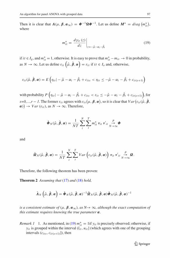
Then it is clear that Λ(μ,β,α∞) = Φ−1Φ−1. Let us define M∗ = diag(m∗i t

),

where

m∗i t =dγi t (z)

dz


(19)

if i t ∈ Ig , and m∗i t = 1, otherwise. It is easy to prove that m∗i t −mit → 0 in probability,

as N →∞. Let us define εi t

(μ, β,α

)= εi t if i t ∈ Io and, otherwise,

εi t (μ, β,α) = E(ηi t | − μ− αi − βt + cits < ηi t ≤ −μ− αi − βt + cit(s+1)

)

with probability P(ηi t | − μ− αi − βt + cits < εi t ≤ −μ− αi − βt + cit(s+1)

), for

s=0,…,r− 1. The former εi t agrees with εi t(μ,β,α

), so it is clear that V ar

(εi t (μ, β,

α))→ V ar (εi t ), as N →∞. Therefore,

ΦN (μ, β,α) = 1

N T

N∑

i

T∑

t

m∗i t vi t v′i tP→

N→∞Φ

and

Ω N (μ, β,α) = 1

N T

N∑

i

T∑

t

V ar(εi t (μ, β,α)

)vi t v′i t

P→N→∞Ω.

Therefore, the following theorem has been proven:

Theorem 2 Assuming that (17) and (18) hold,

ΛN

(μ, β,α

)= ΦN (μ, β,α)−1Ω N (μ, β,α)ΦN (μ, β,α)−1

is a consistent estimate of (μ,β,α∞), as N→∞, although the exact computation ofthis estimate requires knowing the true parameter α.

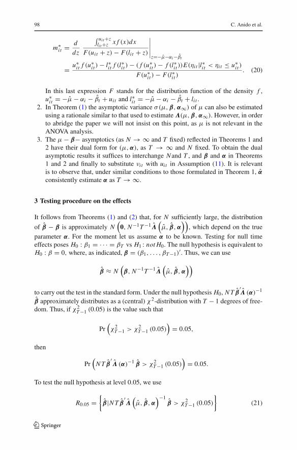
Remark 1 1. As mentioned, in (19) m∗i t = 1if yit is precisely observed; otherwise, ifyit is grouped within the interval (li t , uit ] (which agrees with one of the groupingintervals (cits, cit (s+1)]), then

123

98 C. Anido et al.

m∗i t =d

dz

∫ uit+zli t+z x f (x)dx

F(uit + z)− F(li t + z)

∣∣∣∣∣z=−μ−αi−βt

= u∗i t f (u∗i t )− l∗i t f (l∗i t )− ( f (u∗i t )− f (l∗i t ))E(ηi t |l∗i t < ηi t ≤ u∗i t )F(u∗i t )− F(l∗i t )

. (20)

In this last expression F stands for the distribution function of the density f ,u∗i t = −μ− αi − βt + uit and l∗i t = −μ− αi − βt + li t .

2. In Theorem (1) the asymptotic variance σ(μ,β,α∞) of μ can also be estimatedusing a rationale similar to that used to estimate Λ(μ,β,α∞). However, in orderto abridge the paper we will not insist on this point, as μ is not relevant in theANOVA analysis.

3. The μ− β− asymptotics (as N →∞ and T fixed) reflected in Theorems 1 and2 have their dual form for (μ,α), as T → ∞ and N fixed. To obtain the dualasymptotic results it suffices to interchange Nand T , and β and α in Theorems1 and 2 and finally to substitute νi t with uit in Assumption (11). It is relevantis to observe that, under similar conditions to those formulated in Theorem 1, α

consistently estimate α as T →∞.

3 Testing procedure on the effects

It follows from Theorems (1) and (2) that, for N sufficiently large, the distribution

of β − β is approximately N(

0, N−1T−1Λ(μ, β,α

)), which depend on the true

parameter α. For the moment let us assume α to be known. Testing for null timeeffects poses H0 : β1 = · · · = βT vs H1 : not H0. The null hypothesis is equivalent toH0 : β = 0, where, as indicated, β = (β1, . . . , βT−1)

′. Thus, we can use

β ≈ N(β, N−1T−1Λ

(μ, β,α

))

to carry out the test in the standard form. Under the null hypothesis H0, N T β′Λ (α)−1

β approximately distributes as a (central) χ2-distribution with T − 1 degrees of free-dom. Thus, if χ2

T−1 (0.05) is the value such that

Pr(χ2

T−1 > χ2T−1 (0.05)

)= 0.05,

then

Pr(

N T β′Λ (α)−1 β > χ2

T−1 (0.05))= 0.05.

To test the null hypothesis at level 0.05, we use

R0.05 ={β|N T β

′Λ

(μ, β,α

)−1β > χ2

T−1 (0.05)

}(21)

123


as our critical region. Similarly, to test the null hypothesis at level l (0<l<1), the value0.05 must be substituted by l.

Up to now, we have supposed α to be known, although in fact it is not. We simplypropose to appeal to the consistency (as T → ∞) of α as an estimate of α and tosubstitute Λ(μ, β,α) with Λ(μ, β, α) = Λ(δ). Thus, the strategic plan that we pro-pose to test null time effects when some yit are grouped, is given by the steps 1–3below:

This procedure is also applicable to test for null linear transformations of the timeeffects. For an arbitrary matrix C of rank r ≤ T − 1, we can test H0:Cβ = 0 vsH1 : not H0 at level l by taking

Rl ={β|N T β

′C ′

(CΛ

(δ)

C ′)−1

Cβ > χ2r (l)

}

as the critical region. This follows from the fact that Cβ and N T β′C ′

(CΛ

(δ)

C ′)−1

Cβ approximately distribute as a N(

Cβ, N−1T−1CΛ (α) C ′)

and a central χ2with

r degrees of freedom, respectively.

123

100 C. Anido et al.

Similarly, the procedure may be adapted straightaway to test for either null indi-vidual effects (or null linear transformations of these), and also to test if the constanteffect is equal to a certain value. Nonetheless, we will not insist on this point.

To finish let us highlight a final substantial advantage of the proposed algorithmcompared to the EM for ANOVA purposes. Our proposal bases the hypothesis testingon the computation of the matrix Λ(δ), in which only the first derivatives

m∗i t =d

dzE (ηi t |li t + z < ηi t ≤ uit + z)


are involved. These derivatives do have a closed form, which is similar to (20) aftersubstituting αi with αi . For its part, in the EM environment the matrix

ΛE M

(δE M

) =(−∂2l(δ)

∂δ∂δ′

∣∣∣∣δ=δ

E M

)−1

,

is equivalent to the former Λ(δ) and is equal to the inverse of the Fisher information

matrix evaluated in the convergence point of the EM, δE M

. If f has been standardized,the log-likelihood function agrees with the integral function

l(δ) =∑

i t∈Io

log f (yit − μ− αi − βt )+∑

i t∈Ig

log

ui j−μ−αi−βt∫

li j−μ−αi−β

f (x)dx .

Within the context of the EM algorithm, several methods have been proposed toevaluate the Hessian (matrix) of the log-likelihood function. Among them, the directnumerical differentiation (Meilijson 1989), the Louis′ (1982) method or the proposalof Meng and Rubin (1991) which uses the EM iterates. In all of these methods theevaluation of the second derivatives of l(δ) is numerical and quite unstable. Undoubt-

edly the computation of Λ(δ) is easier and more reliable than that of ΛE M

(δE M

) ifwe recall that only first derivatives in analytical form are required.

4 Simulations and computational results

In this section, we present a simulation study carried out to analyse the performanceof the testing procedure commented on above. Our focus is on testing for constanttime effects, since testing for constant individual effects is similar. We have fixedT = 4, and the values μ+ αi (i = 1, . . . , N ) were selected uniformly on the interval(−5, 5) for different values of N (N = 15, 25, 50), as a way of testing the rate ofconvergence of the asymptotic distributions stated in Theorem 1. In each case, μ andthe α′i s were calculated from the values ϕi . Then, several sets of values were assignedto (β1, β2, β3, β4). The first was (0, 0, 0, 0), since the interest was to test for constanttime factors. The remaining sets are included in Table 1, where it can be seen that they

123


differ increasingly from the initial null vector, the intention being to evaluate the testpower function on different points. Finally, we generated the errors from the followingdistributions: (a) Laplace (1), with the density function f (u) = 2−1exp(−|u|); (b)Logistic, with f (u) = e−u(1 + e−u)−2; and (c) N (0, 1). Once the dependent vari-ables were generated from model (1), each yit was grouped with probability 0.5, inwhich case the grouping intervals were ( −∞,−5], (−5, 0], and ( 0,∞). With theresulting data, we have implemented the testing procedure shown in Sect. 3. First,we have run the estimating algorithm to determine the complete parameter estimate

δ = (μ, α′, β′)′ as the limit point of the sequence generated by the algorithm, {δ p};

we used the STOP condition ||δ p−δ p−1||2 ≤ 10−5, and the starting point of the algo-rithm was randomly selected from a uniform distribution on (−3, 3)N+T−1, althoughδ is independent of the starting point, as proved in Theorem 1. Then, the estimate,Λ(δ), of the asymptotic covariance matrix of β was computed. Finally, we have com-

puted N T β′Λ(δ)−1β, which allows us to determine the critical region Rl for testing

H0:β1 = · · · = β4vsH1 : not H0 at level l. These processes were repeated 300 times,

and we recorded the values δ(r)

, Λ(r)(δ(r)

), and N T β(r)′

Λ(r)

(δ(r)

)−1β(r)

, correspond-ing to the replication r (r = 1, . . . , 300). The results that we have obtained concerningthe time-dependent parameters are synthesised in Table 1. This includes the empiricalmultivariate mean square errors (MSE)

E

(∥∥∥β − β

∥∥∥

2)= 300−1

300∑

r=1

∥∥∥β

(r) − β

∥∥∥

2.

For purposes of comparison Table 1 also shows the former MSE for two usual ordinaryleast squares estimates. The first takes into account all the yit -values, before being sub-

mitted to the grouping process, and it will be denoted by β(r)O L S

in the sequel. The

second estimate, which will be identified by β(r)ols

(with the super-index writtenin small letters) was computed considering only the non-grouped data, after havingdischarged the resulting grouped yit -values, in each replication.

Upon examination of Table 1, the following remarks are sketched. The MSE′s of allof the estimates decrease as the number of individuals increases. Thus naturally, theprecision of the time parameter estimates is improved in all cases by increasing N . The

estimate βO L S

, which uses the complete data before executing the censoring process,has the minimum empirical MSE for all of the error distributions mentioned above. For

its part, the maximum MSE is achieved by βols

, which discharges all the censored data.

The increases between their respective MSE, E∥∥∥β

ols − β

∥∥∥

2 − E∥∥∥β

O L S − β

∥∥∥

2, can

be attributed to the censoring information loss. The estimating algorithm described inSect. 2 substantially diminishes the increase of MSE due to the information loss. In thepresence of the information loss that derives from the data grouping process mentionedabove, the rate of improvement of our estimate β compared with the ols-estimate, isgiven by

123

102 C. Anido et al.

Table 1 Mean square errors of the different estimates for different error distributions, number of individ-uals, and true values of β

Estimates Error distribution and number of individualsobtained from

Laplace Standard normal Logistic

N = 15 N = 25 N = 50 N = 15 N = 25 N = 50 N = 15 N = 25 N = 50

True time parameters: β1 = 0, β2 = 0, β3 = 0, β4 = 0

OLS 0.2832 0.1592 0.0812 0.1149 0.0699 0.0396 0.4709 0.2642 0.1335

ols 0.4684 0.2373 0.1197 0.4579 0.3791 0.3306 0.7418 0.3778 0.1893

Proposed algorithm 0.3854 0.2135 0.1071 0.3120 0.2180 0.1804 0.5826 0.3059 0.1617

True time parameters: β1 = 0, β2 = 0, β3 = 0.2, β4 = −0.2

OLS 0.2875 0.1543 0.0815 0.1102 0.0822 0.0400 0.4784 0.2656 0.1345

ols 0.4689 0.2309 0.1222 0.4500 0.3787 0.3267 0.7469 0.3770 0.1798



OLS 0.2899 0.1535 0.0824 0.1067 0.0721 0.0424 0.4503 0.2598 0.1321

ols 0.4675 0.2311 0.1201 0.4489 0.3781 0.3212 0.7284 0.3635 0.1579



OLS 0.2865 0.1498 0.0856 0.1079 0.0862 0.0491 0.4639 0.2643 0.1298

ols 0.4600 0.2287 1.1145 0.4498 0.3772 0.3280 0.7312 0.3701 0.1793



OLS 0.2799 0.1507 0.0832 0.1103 0.0678 0.0389 0.4629 0.2687 0.1328

ols 0.4578 0.2299 0.1124 0.4521 0.3698 0.3301 0.7408 0.3659 0.1894


True time parameters: β1 = 0.2, β2 = −0.2, β3 = 0.4, β4 = −0.4

OLS 0.2903 0.1589 0.0901 0.1001 0.0781 0.0521 0.4498 0.2559 0.1279

ols 0.4706 0.2401 0.1199 0.4398 0.3689 0.3199 0.7198 0.3598 0.1603


True time parameters: β1 = 1, β2 = −2, β3 = 0, β4 = 1

OLS 0.2850 0.1612 0.0828 0.0987 0.0891 0.0394 0.4902 0.2612 0.1343

ols 0.4699 0.2381 0.1178 0.4324 0.3723 0.3000 0.7534 0.3699 0.1753


True time parameters: β1 = −5, β2 = 4, β3 = 2, β4 = −1

OLS 0.2901 0.1587 0.0907 0.1064 0.0805 0.0502 0.4879 0.2679 0.1321

ols 0.4725 0.2456 0.1235 0.4401 0.3703 0.3240 0.7600 0.3823 0.1783


100

⎛

⎜⎝

E∥∥∥β

ols − β

∥∥∥

2 − E∥∥∥β − β

∥∥∥

2

E∥∥∥β

ols − β

∥∥∥2 − E

∥∥∥βO L S − β

∥∥∥2

⎞

⎟⎠ %. (24)

123


Table 2 Rate of improvement from expression (14) in the text of β with respect to βols

(in %)

True time parametersβ = (β1, β2, β3)′;thus, β4 = −β1− β2 − β3

Error distribution and number of individuals


N = 15 N = 25 N = 50 N = 15 N = 25 N = 50 N = 15 N = 25 N = 50

β = (0, 0, 0)′ 44.82 30.47 32.73 42.54 52.10 51.62 58.77 63.29 49.46

β = (0.2, 0, 0)′ 45.70 36.42 38.33 43.00 56.09 52.04 60.26 68.76 49.45

β = (0.4, 0, 0)′ 41.27 38.79 39.79 45.59 57.32 52.83 59.76 68.66 40.31

β = (0.6, 0, 0)′ 40.06 37.26 35.29 45.04 58.35 55.50 57.35 60.11 55.96

β = (0.8, 0, 0)′ 41.09 37.25 33.90 44.76 54.54 53.40 60.27 71.81 49.29

β = (0.2,−0.2, 0.4)′ 35.55 34.61 28.86 46.66 57.22 55.04 69.15 69.39 36.11

β = (1,−2, 0)′ 41.27 29.52 30.29 50.34 56.81 56.83 51.29 61.55 42.68

β = (−5, 4, 2)′ 34.32 27.73 34.45 49.24 58.42 58.11 51.19 49.83 41.56

(b) Normal errors Logistic errors

0.0

Laplacian errors(a) (c)

Fig. 1 Cross-section of the empirical test power function, φ(β1, β2,0), when N = 25

Table 2 shows this rate when, as in Table 1, we vary (1) the error distribution, (2) thenumber of individuals, N , and (3) the true time-dependent parameters.

Additionally, we have tested the hypothesis H0 :β = 0 vs H1 :β �= 0 with the pro-cedure proposed in Sect. 3, and then we have computed the number, M,of replicationswhere χ2-tests commented on in this section led us to reject the null hypothesis, atlevel 0.05. Clearly, M agrees with the number of replications r for which the inequality

N T β(r)′

Λ(r)(δ(r)

)−1β(r)

> 7.815

is fulfilled, as χ23 (0.05) = 7.815. The fraction M/300 represents the empirical test

power function, φ(.), in the true value of β. As β varies, this fraction empiricallyestimates the probability of the Type I error when β = 0, otherwise, it estimates 1minus the probability of the Type II errors.

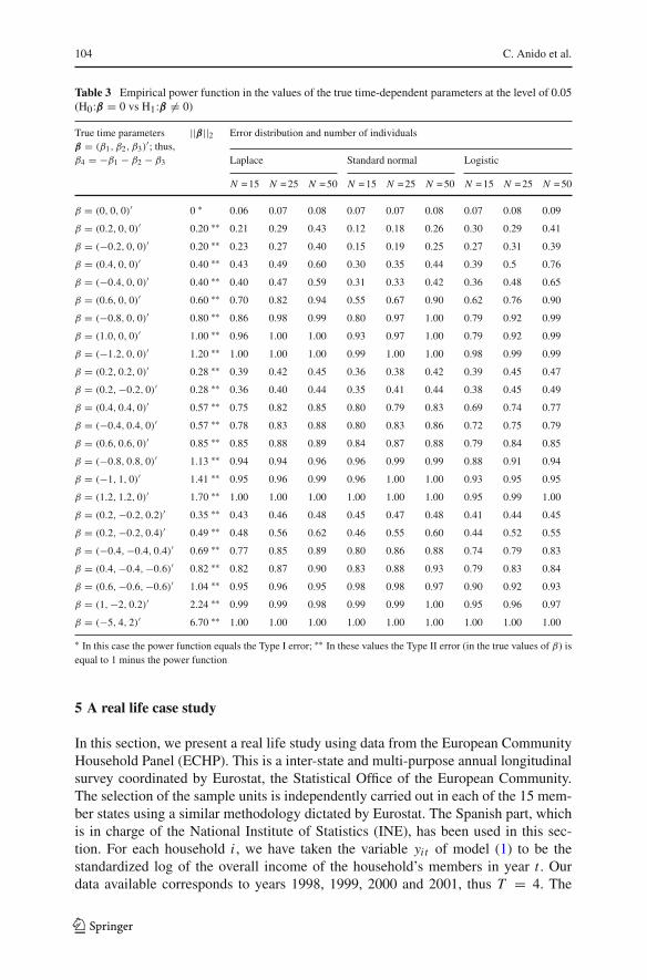
Figure 1 depicts the cross-section (assuming β3 = 0) of the empirical test powerfunction, when N = 25, for the three error distributions which were considered in thissection. Certain values of this cross-section, φ(β1,β2,0), are included in the first andthird horizontal data parts of Table 3.

123

104 C. Anido et al.

Table 3 Empirical power function in the values of the true time-dependent parameters at the level of 0.05(H0:β = 0 vs H1:β �= 0)

True time parametersβ = (β1, β2, β3)

′; thus,β4 = −β1 − β2 − β3

||β||2 Error distribution and number of individuals


N = 15 N = 25 N = 50 N = 15 N = 25 N = 50 N = 15 N = 25 N = 50

β = (0, 0, 0)′ 0 ∗ 0.06 0.07 0.08 0.07 0.07 0.08 0.07 0.08 0.09

β = (0.2, 0, 0)′ 0.20 ∗∗ 0.21 0.29 0.43 0.12 0.18 0.26 0.30 0.29 0.41

β = (−0.2, 0, 0)′ 0.20 ∗∗ 0.23 0.27 0.40 0.15 0.19 0.25 0.27 0.31 0.39

β = (0.4, 0, 0)′ 0.40 ∗∗ 0.43 0.49 0.60 0.30 0.35 0.44 0.39 0.5 0.76

β = (−0.4, 0, 0)′ 0.40 ∗∗ 0.40 0.47 0.59 0.31 0.33 0.42 0.36 0.48 0.65

β = (0.6, 0, 0)′ 0.60 ∗∗ 0.70 0.82 0.94 0.55 0.67 0.90 0.62 0.76 0.90

β = (−0.8, 0, 0)′ 0.80 ∗∗ 0.86 0.98 0.99 0.80 0.97 1.00 0.79 0.92 0.99

β = (1.0, 0, 0)′ 1.00 ∗∗ 0.96 1.00 1.00 0.93 0.97 1.00 0.79 0.92 0.99

β = (−1.2, 0, 0)′ 1.20 ∗∗ 1.00 1.00 1.00 0.99 1.00 1.00 0.98 0.99 0.99

β = (0.2, 0.2, 0)′ 0.28 ∗∗ 0.39 0.42 0.45 0.36 0.38 0.42 0.39 0.45 0.47

β = (0.2,−0.2, 0)′ 0.28 ∗∗ 0.36 0.40 0.44 0.35 0.41 0.44 0.38 0.45 0.49

β = (0.4, 0.4, 0)′ 0.57 ∗∗ 0.75 0.82 0.85 0.80 0.79 0.83 0.69 0.74 0.77

β = (−0.4, 0.4, 0)′ 0.57 ∗∗ 0.78 0.83 0.88 0.80 0.83 0.86 0.72 0.75 0.79

β = (0.6, 0.6, 0)′ 0.85 ∗∗ 0.85 0.88 0.89 0.84 0.87 0.88 0.79 0.84 0.85

β = (−0.8, 0.8, 0)′ 1.13 ∗∗ 0.94 0.94 0.96 0.96 0.99 0.99 0.88 0.91 0.94

β = (−1, 1, 0)′ 1.41 ∗∗ 0.95 0.96 0.99 0.96 1.00 1.00 0.93 0.95 0.95

β = (1.2, 1.2, 0)′ 1.70 ∗∗ 1.00 1.00 1.00 1.00 1.00 1.00 0.95 0.99 1.00

β = (0.2,−0.2, 0.2)′ 0.35 ∗∗ 0.43 0.46 0.48 0.45 0.47 0.48 0.41 0.44 0.45

β = (0.2,−0.2, 0.4)′ 0.49 ∗∗ 0.48 0.56 0.62 0.46 0.55 0.60 0.44 0.52 0.55

β = (−0.4,−0.4, 0.4)′ 0.69 ∗∗ 0.77 0.85 0.89 0.80 0.86 0.88 0.74 0.79 0.83

β = (0.4,−0.4,−0.6)′ 0.82 ∗∗ 0.82 0.87 0.90 0.83 0.88 0.93 0.79 0.83 0.84

β = (0.6,−0.6,−0.6)′ 1.04 ∗∗ 0.95 0.96 0.95 0.98 0.98 0.97 0.90 0.92 0.93

β = (1,−2, 0.2)′ 2.24 ∗∗ 0.99 0.99 0.98 0.99 0.99 1.00 0.95 0.96 0.97

β = (−5, 4, 2)′ 6.70 ∗∗ 1.00 1.00 1.00 1.00 1.00 1.00 1.00 1.00 1.00

∗ In this case the power function equals the Type I error; ∗∗ In these values the Type II error (in the true values of β) isequal to 1 minus the power function

5 A real life case study

In this section, we present a real life study using data from the European CommunityHousehold Panel (ECHP). This is a inter-state and multi-purpose annual longitudinalsurvey coordinated by Eurostat, the Statistical Office of the European Community.The selection of the sample units is independently carried out in each of the 15 mem-ber states using a similar methodology dictated by Eurostat. The Spanish part, whichis in charge of the National Institute of Statistics (INE), has been used in this sec-tion. For each household i , we have taken the variable yit of model (1) to be thestandardized log of the overall income of the household’s members in year t . Ourdata available corresponds to years 1998, 1999, 2000 and 2001, thus T = 4. The

123


number of different households sampled was 6,233. However, not all of these wereobserved in the 4 years, since certain households are created and destroyed in eachperiod. Thus, our data is an incomplete panel, and we have treated missing data asgrouped on the whole line. The number of missing observations was 4,194, which rep-resents the 16.8% of the 24,932 possible observations (6,233 households×4 years). Inaddition to this, in 4.2% of the households with several active members, the incomesof some of these members are lacking. This means that the total incomes of thesehouseholds are in fact right censored. Finally, we have assumed in this study thatthe error terms of model (1) are normal. Our goal has been to test the hypothesesH0 :β1 = β2 = β3 = 0 against H1: not H0, through the proposed algorithm. This

gives the limit point β =(β1, β2, β3

)and it also yields as a sub-product the asymp-

totic covariance matrix of β, which was denoted by Λ(δ)

in the description of the

algorithm included in Sect. 3. Finally, to test H0 against H1 at the l-significance-level, we have used as our critical region Rl given in (23), within the aforementioneddescription of the algorithm.

Part (a) of Table 4 shows the results obtained, including the time parameter esti-

mates, their asymptotic covariance matrix, the value of the test statistic N T β′Λ(δ)β

included in Rl and also the p values for testing that that there is no time effect. It canbe seen that the value of the test statistic with our proposed algorithm was 158.22 (pvalue equal to 0.000). Thus, there is the strongest evidence that the time parametersof model (1) differ from 1 year to other.

All of the former computations were repeated with two special sub-samples, namely,one-person households (1,048 sampled households, with a 13.55% of missing data andnone of the right censored incomes) and households composed of a couple withoutdependent children (2,272 observations over the 4 years, with 24.82% of missing dataand a 5.2% of censored incomes). Parts (b) and (c) of Table 4 are similar to part (a),although referred to these sub-samples. For the first sub-sample the p value resulted in0.319; thus, the hypothesis of null time effects is accepted at any level of significancelower than this. On the contrary, for the second sub-sample the same hypothesis isrejected at both the 5 and 1% level of significance, as the value 14.24 of the test statisticcorresponds to a p value of 0.002.

6 Concluding remarks

In this paper, we have presented an algorithm useful in analysing the variance ofgrouped and ungrouped panel data. The algorithm jointly tackles two estimating tasks.The first is dedicated to the estimation of the parameters of model (1) through an itera-tive procedure which is rather easy to implement, as it only involves the simple expres-sions (8)–(10). It is proven that the iterative procedure converges to a unique fixedpoint whichever starting point is taken. This unique limit point defines our estimate.The second task faces the estimation of the covariance matrix of the time (individual)parameters from expression (22), which is not complicated since it only involves a sim-ple differentiation and a little algebra. The aforementioned covariance matrix is thenused to test null linear combinations of the time (individual) dependent parameters.

123

106 C. Anido et al.

Table 4 Performance of the proposed algorithm on the ECHP data

(a) Using the total sample of households1. Time parameter estimates:

β = (β1, β2, β3), β4 = −β1 − β2 − β3 (−0.123,−0.024, 0.044), 0.103

2. Asymptotic covariance matrix: Λ(δ)

⎛

⎝3.504 −1.118 −1.180−1.403 3.561 −1.212−1.175 −1.206 3.699

⎞

⎠

3. Value of the test statistic N T β′Λ(δ)−1β 158.221

4. p value 0.000

5. The hypothesis H0 (constant time effects) is Rejected∗(b) Using the sub-sample of one-person households1. Time parameter estimates:

β = (β1, β2, β3), β4 = −β1 − β2 − β3 (−0.012, 0.070,−0.095), 0.037


⎛

⎝3.780 −1.332 −1.308−1.332 3.529 −1.173−1.308 −1.173 3.490

⎞

⎠


4. p value 0.319

5. The hypothesis H0 (constant time effects) is Accepted∗(c) Using the sub-sample ofhousehold composed by a couplewithout children1. Time parameter estimates:

β = (β1, β2, β3), β4 = −β1 − β2 − β3 (−0.160, 0.002, 0.080), 0.078


⎛

⎝5.023 −2.034 −1.643−2.034 4.362 −1.392−1.643 −1.392 3.864

⎞

⎠


4. p value 0.002

5. The hypothesis H0 (constant time effects) is Rejected∗∗At both the 5 and 1% level of significance (χ2

3,0.05 = 7.815 or χ23,0.01 = 11.340)

In spite of the simplicity of the algorithm, the results shown in Sect. 4 indicate thatit is rather efficient in comparison to some alternative procedures. In fact, its level ofefficiency is of the same order as the standard ANOVA in absence of grouped data,although the algorithm is designed to handle grouped or missing data, as has beenindicated. This means that the loss of accuracy due to existence of incomplete data israther mitigated by the proposed algorithm. Also, we have shown that standard statis-tical methods based on discharging the existing incomplete data worsen our results.

Finally, in Sect. 5 we included a real life case study regarding the analysis of vari-ance of household incomes taken from the ECHP (European Community HouseholdPanel).

Acknowledgments This paper stems from research partially funded by MEC and EUROSTAT, undergrant MTM2004-05776 and Contract No 9.242.010, respectively.

123


References

An MY (1998) Logconcavity versus logconvexity: a complete characterization. J Econ Theory 80:350–369

Baltagi BH (1995) Econometric analysis of panel data. Wiley, New YorkDempster AP, Laird NM, Rubin DB (1977) Maximum likelihood from incomplete data via the EM algo-

rithm. J R Stat Soc 39(B):1–22Healy MJR, Westmacott M (1956) Missing values in experiments analysed on automatic computers. Appl

Stat 5:203–206Hsiao C (2003) Analysis of panel data. Cambridge University Press, CambridgeLaha RG, Rohatgi VK (1979) Probability theory. Wiley, New YorkLange K (1999) Numerical analysis for statistician. Springer, BerlinLittle RJA, Rubin DB (1987) Statistical analysis with missing data. Wiley, New YorkLouis TA (1982) Finding observed information using the EM algorithm. J R Stat Soc 44(B):98–130McLachlan GJ, Krishnan T (1997) The EM algorithm and extensions. Wiley, New YorkMeilijson I (1989) A fast improvement of the EM algorithm on its own terms. J R Stat Soc 51(B):127–138Orchard T, Woodbury MA (1972) A missing information principle: theory and applications. In:

Proceedings of the sixth berkeley symposium on mathematical statistics and probability. Universityof California Press, Berkeley, pp 697–715

Meng XL, Rubin DB (1991) Using EM to obtain asymptotic variance-covariance matrices. J Am Stat Assoc86:899–909

Tanner MA (1993) Tools for statistical inference Methods for the exploration of posterior distributions andlikelihood functions. Springer, Berlin

123

An algorithm for panel ANOVA with grouped data

Documents

Transcript of An algorithm for panel ANOVA with grouped data