Grouped Mathematically Differentiable NMS for Monocular 3D ...
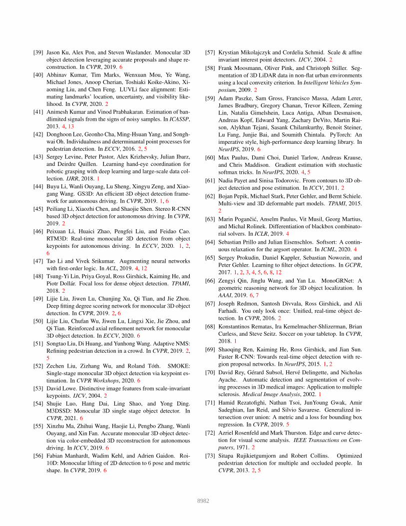
11
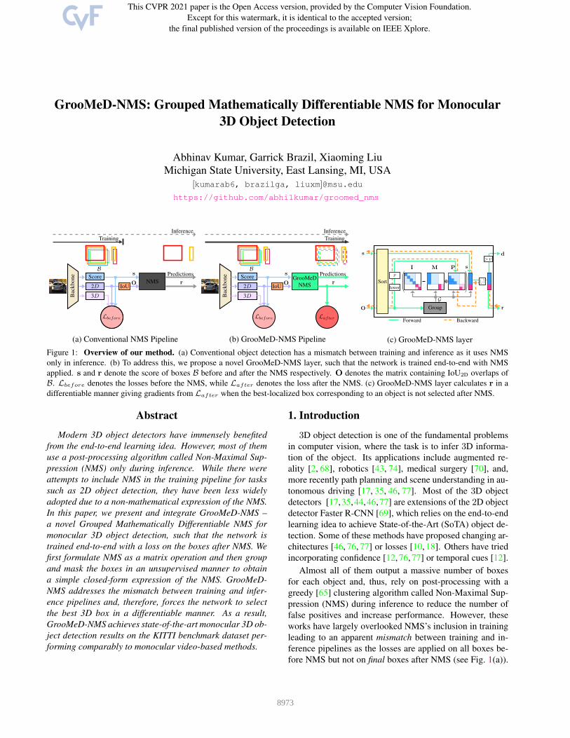
GrooMeD-NMS: Grouped Mathematically Differentiable NMS for Monocular 3D Object Detection Abhinav Kumar, Garrick Brazil, Xiaoming Liu Michigan State University, East Lansing, MI, USA [kumarab6, brazilga, liuxm]@msu.edu https://github.com/abhi1kumar/groomed_nms Backbone Score 2D 3D s O IoU Lbefore B Inference NMS Predictions r Training Lbefore (a) Conventional NMS Pipeline Backbone Score 2D 3D s O IoU Lbefore B Inference GrooMeD NMS Predictions r Training Laf ter (b) GrooMeD-NMS Pipeline s s O Sort Group G lower p I M P ⌊.⌉ r >v d Forward Backward (c) GrooMeD-NMS layer Figure 1: Overview of our method. (a) Conventional object detection has a mismatch between training and inference as it uses NMS only in inference. (b) To address this, we propose a novel GrooMeD-NMS layer, such that the network is trained end-to-end with NMS applied. s and r denote the score of boxes B before and after the NMS respectively. O denotes the matrix containing IoU2D overlaps of B. L before denotes the losses before the NMS, while L af ter denotes the loss after the NMS. (c) GrooMeD-NMS layer calculates r in a differentiable manner giving gradients from L af ter when the best-localized box corresponding to an object is not selected after NMS. Abstract Modern 3D object detectors have immensely benefited from the end-to-end learning idea. However, most of them use a post-processing algorithm called Non-Maximal Sup- pression (NMS) only during inference. While there were attempts to include NMS in the training pipeline for tasks such as 2D object detection, they have been less widely adopted due to a non-mathematical expression of the NMS. In this paper, we present and integrate GrooMeD-NMS – a novel Grouped Mathematically Differentiable NMS for monocular 3D object detection, such that the network is trained end-to-end with a loss on the boxes after NMS. We first formulate NMS as a matrix operation and then group and mask the boxes in an unsupervised manner to obtain a simple closed-form expression of the NMS. GrooMeD- NMS addresses the mismatch between training and infer- ence pipelines and, therefore, forces the network to select the best 3D box in a differentiable manner. As a result, GrooMeD-NMS achieves state-of-the-art monocular 3D ob- ject detection results on the KITTI benchmark dataset per- forming comparably to monocular video-based methods. 1. Introduction 3D object detection is one of the fundamental problems in computer vision, where the task is to infer 3D informa- tion of the object. Its applications include augmented re- ality [2, 68], robotics [43, 74], medical surgery [70], and, more recently path planning and scene understanding in au- tonomous driving [17, 35, 46, 77]. Most of the 3D object detectors [17, 35, 44, 46, 77] are extensions of the 2D object detector Faster R-CNN [69], which relies on the end-to-end learning idea to achieve State-of-the-Art (SoTA) object de- tection. Some of these methods have proposed changing ar- chitectures [46, 76, 77] or losses [10, 18]. Others have tried incorporating confidence [12, 76, 77] or temporal cues [12]. Almost all of them output a massive number of boxes for each object and, thus, rely on post-processing with a greedy [65] clustering algorithm called Non-Maximal Sup- pression (NMS) during inference to reduce the number of false positives and increase performance. However, these works have largely overlooked NMS’s inclusion in training leading to an apparent mismatch between training and in- ference pipelines as the losses are applied on all boxes be- fore NMS but not on final boxes after NMS (see Fig. 1(a)). 8973
-
Upload
khangminh22 -
Category
Documents
-
view
3 -
download
0
Transcript of Grouped Mathematically Differentiable NMS for Monocular 3D ...
GrooMeD-NMS: Grouped Mathematically Differentiable NMS for Monocular
3D Object Detection
Abhinav Kumar, Garrick Brazil, Xiaoming Liu
Michigan State University, East Lansing, MI, USA
[kumarab6, brazilga, liuxm]@msu.edu
https://github.com/abhi1kumar/groomed_nms
Bac
kb
on
e Score
2D
3D
s
OIoU
Lbefore
B
Inference
NMS
Predictions
r
Training
Lbefore
(a) Conventional NMS Pipeline
Bac
kb
on
e Score
2D
3D
s
OIoU
Lbefore
B
Inference
GrooMeD
NMS
Predictions
r
Training
Lafter
(b) GrooMeD-NMS Pipeline
s
s
O
Sort
Group
G
lower
p
I M P
⌊.⌉
r
>vd
Forward Backward
(c) GrooMeD-NMS layer
Figure 1: Overview of our method. (a) Conventional object detection has a mismatch between training and inference as it uses NMS
only in inference. (b) To address this, we propose a novel GrooMeD-NMS layer, such that the network is trained end-to-end with NMS
applied. s and r denote the score of boxes B before and after the NMS respectively. O denotes the matrix containing IoU2D overlaps of
B. Lbefore denotes the losses before the NMS, while Lafter denotes the loss after the NMS. (c) GrooMeD-NMS layer calculates r in a
differentiable manner giving gradients from Lafter when the best-localized box corresponding to an object is not selected after NMS.
Abstract
Modern 3D object detectors have immensely benefited
from the end-to-end learning idea. However, most of them
use a post-processing algorithm called Non-Maximal Sup-
pression (NMS) only during inference. While there were
attempts to include NMS in the training pipeline for tasks
such as 2D object detection, they have been less widely
adopted due to a non-mathematical expression of the NMS.
In this paper, we present and integrate GrooMeD-NMS –
a novel Grouped Mathematically Differentiable NMS for
monocular 3D object detection, such that the network is
trained end-to-end with a loss on the boxes after NMS. We
first formulate NMS as a matrix operation and then group
and mask the boxes in an unsupervised manner to obtain
a simple closed-form expression of the NMS. GrooMeD-
NMS addresses the mismatch between training and infer-
ence pipelines and, therefore, forces the network to select
the best 3D box in a differentiable manner. As a result,
GrooMeD-NMS achieves state-of-the-art monocular 3D ob-
ject detection results on the KITTI benchmark dataset per-
forming comparably to monocular video-based methods.
1. Introduction
3D object detection is one of the fundamental problems
in computer vision, where the task is to infer 3D informa-
tion of the object. Its applications include augmented re-
ality [2, 68], robotics [43, 74], medical surgery [70], and,
more recently path planning and scene understanding in au-
tonomous driving [17, 35, 46, 77]. Most of the 3D object
detectors [17,35,44,46,77] are extensions of the 2D object
detector Faster R-CNN [69], which relies on the end-to-end
learning idea to achieve State-of-the-Art (SoTA) object de-
tection. Some of these methods have proposed changing ar-
chitectures [46, 76, 77] or losses [10, 18]. Others have tried
incorporating confidence [12, 76, 77] or temporal cues [12].
Almost all of them output a massive number of boxes
for each object and, thus, rely on post-processing with a
greedy [65] clustering algorithm called Non-Maximal Sup-
pression (NMS) during inference to reduce the number of
false positives and increase performance. However, these
works have largely overlooked NMS’s inclusion in training
leading to an apparent mismatch between training and in-
ference pipelines as the losses are applied on all boxes be-
fore NMS but not on final boxes after NMS (see Fig. 1(a)).
8973

We also find that 3D object detection suffers a greater mis-
match between classification and 3D localization compared
to that of 2D localization, as discussed further in Sec. A3.2
of the supplementary and observed in [12, 35, 76]. Hence,
our focus is 3D object detection.
Earlier attempts to include NMS in the training
pipeline [31,32,65] have been made for 2D object detection
where the improvements are less visible. Recent efforts to
improve the correlation in 3D object detection involve cal-
culating [77, 79] or predicting [12, 76] the scores via like-
lihood estimation [40] or enforcing the correlation explic-
itly [35]. Although this improves the 3D detection perfor-
mance, improvements are limited as their training pipeline
is not end to end in the absence of a differentiable NMS.
To address the mismatch between training and inference
pipelines as well as the mismatch between classification and
3D localization, we propose including the NMS in the train-
ing pipeline, which gives a useful gradient to the network
so that it figures out which boxes are the best-localized in
3D and, therefore, should be ranked higher (see Fig. 1(b)).
An ideal NMS for inclusion in the training pipeline
should be not only differentiable but also parallelizable.
Unfortunately, the inference-based classical NMS and Soft-
NMS [8] are greedy, set-based and, therefore, not paralleliz-
able [65]. To make the NMS parallelizable, we first for-
mulate the classical NMS as matrix operation and then ob-
tain a closed-form mathematical expression using elemen-
tary matrix operations such as matrix multiplication, ma-
trix inversion, and clipping. We then replace the threshold
pruning in the classical NMS with its softer version [8] to
get useful gradients. These two changes make the NMS
GPU-friendly, and the gradients are backpropagated. We
next group and mask the boxes in an unsupervised man-
ner, which removes the matrix inversion and simplifies our
proposed differentiable NMS expression further. We call
this NMS as Grouped Mathematically Differentiable Non-
Maximal Suppression (GrooMeD-NMS).
In summary, the main contributions of this work include:
• This is the first work to propose and integrate a closed-
form mathematically differentiable NMS for object de-
tection, such that the network is trained end-to-end
with a loss on the boxes after NMS.
• We propose an unsupervised grouping and masking on
the boxes to remove the matrix inversion in the closed-
form NMS expression.
• We achieve SoTA monocular 3D object detection per-
formance on the KITTI dataset performing compara-
bly to monocular video-based methods.
2. Related Work
3D Object Detection. Recent success in 2D object detec-
tion [26, 27, 48, 67, 69] has inspired people to infer 3D in-
formation from a single 2D (monocular) image. How-
ever, the monocular problem is ill-posed due to the inherent
scale/depth ambiguity [82]. Hence, approaches use addi-
tional sensors such as LiDAR [35,75,88], stereo [45,87] or
radar [58, 84]. Although LiDAR depth estimations are ac-
curate, LiDAR data is sparse [33] and computationally ex-
pensive to process [82]. Moreover, LiDARs are expensive
and do not work well in severe weather [82].
Hence, there have been several works on monocular
3D object detection. Earlier approaches [15, 23, 61, 62] use
hand-crafted features, while the recent ones are all based
on deep learning. Some of these methods have proposed
changing architectures [46, 49, 82] or losses [10, 18]. Oth-
ers have tried incorporating confidence [12,49,76,77], aug-
mentation [80], depth in convolution [10, 22] or temporal
cues [12]. Our work proposes to incorporate NMS in the
training pipeline of monocular 3D object detection.
Non-Maximal Suppression. NMS has been used to re-
duce false positives in edge detection [72], feature point
detection [29, 53, 57], face detection [85], human detec-
tion [11, 13, 20] as well as SoTA 2D [26, 48, 67, 69] and
3D detection [4, 12, 17, 76, 77, 82]. Modifications to NMS
in 2D detection [8, 21, 31, 32, 65], 2D pedestrian detec-
tion [42,51,73], 2D salient object detection [91] and 3D de-
tection [76] can be classified into three categories – infer-
ence NMS [8, 76], optimization-based NMS [3, 21, 42, 73,
86, 91] and neural network based NMS [30–32, 51, 65].
The inference NMS [8] changes the way the boxes are
pruned in the final set of predictions. [76] uses weighted av-
eraging to update the z-coordinate after NMS. [73] solves
quadratic unconstrained binary optimization while [3, 42,
81] and [91] use point processes and MAP based inference
respectively. [21] and [86] formulate NMS as a structured
prediction task for isolated and all object instances respec-
tively. The neural network NMS use a multi-layer net-
work and message-passing to approximate NMS [31,32,65]
or to predict the NMS threshold adaptively [51]. [30] ap-
proximates the sub-gradients of the network without mod-
elling NMS via a transitive relationship. Our work pro-
poses a grouped closed-form mathematical approximation
of the classical NMS and does not require multiple layers
or message-passing. We detail these differences in Sec. 4.2.
3. Background
3.1. Notations
Let B= {bi}ni=1 denote the set of boxes or proposals bi
from an image. Let s = {si}ni=1 and r = {ri}
ni=1 denote
their scores (before NMS) and rescores (updated scores af-
ter NMS) respectively such that ri, si ≥ 0 ∀ i. D denotes
the subset of B after the NMS. Let O = [oij ] denote the
n × n matrix with oij denoting the 2D Intersection over
Union (IoU2D) of bi and bj . The pruning function p decides
how to rescore a set of boxes B based on IoU2D overlaps
8974

Algorithm 1: Classical/Soft-NMS [8]
Input: s: scores, O: IoU2D matrix, Nt: NMS threshold,
p: pruning function, τ : temperature
Output: d: box index after NMS, r: scores after NMS
1 begin
2 d← {}3 t← {1, · · · , |s|} ⊲ All box indices
4 r← s
5 while t 6= empty do
6 ν ← argmax r[t] ⊲ Top scored box
7 d← d ∪ ν ⊲ Add to valid box index
8 t← t− ν ⊲ Remove from t
9 for i← 1 : |t| do
10 ri ← (1− pτ (O[ν, i]))ri ⊲ Rescore
11 end
12 end
13 end
of its neighbors, sometimes suppressing boxes entirely. In
other words, p(oi) = 1 denotes the box bi is suppressed
while p(oi) = 0 denotes bi is kept in D. The NMS thresh-
old Nt is the threshold for which two boxes need in order
for the non-maximum to be suppressed. The temperature τ
controls the shape of the exponential and sigmoidal prun-
ing functions p. v thresholds the rescores in GrooMeD and
Soft-NMS [9] to decide if the box remains valid after NMS.
B is partitioned into different groups G = {Gk}. BGk
denotes the subset of B belonging to group k. Thus, BGk=
{bi} ∀ bi ∈ Gk and BGk∩ BGl
= φ ∀ k 6= l. Gk in the
subscript of a variable denotes its subset corresponding to
BGk. Thus, sGk
and rGkdenote the scores and the rescores
of BGkrespectively. α denotes the maximum group size.
∨ denotes the logical OR while ⌊x⌉ denotes clipping of
x in the range [0, 1]. Formally,
⌊x⌉ =
1, x > 1
x, 0 ≤ x ≤ 1
0, x < 0
(1)
|s| denotes the number of elements in s. ❧❧ in the subscript
denotes the lower triangular version of the matrix without
the principal diagonal. ⊙ denotes the element-wise multi-
plication. I denotes the identity matrix.
3.2. Classical and SoftNMS
NMS is one of the building blocks in object detection
whose high-level goal is to iteratively suppress boxes which
have too much IoU with a nearby high-scoring box. We first
give an overview of the classical and Soft-NMS [8], which
are greedy and used in inference. Classical NMS uses the
idea that the score of a box having a high IoU2D overlap
with any of the selected boxes should be suppressed to zero.
That is, it uses a hard pruning p without any temperature τ .
Soft-NMS makes this pruning soft via temperature τ . Thus,
Algorithm 2: GrooMeD-NMS
Input: s: scores, O: IoU2D matrix, Nt: NMS threshold,
p: pruning function, v: valid box threshold, α:
maximum group size
Output: d: box index after NMS, r: scores after NMS
1 begin
2 s, index← sort(s, descending= True) ⊲ Sort s
3 O← O[index][:, index] ⊲ Sort O
4 O ❧❧ ← lower(O) ⊲ Lower △ular matrix
5 P← p(O ❧❧ ) ⊲ Prune matrix
6 I← Identity(|s|) ⊲ Identity matrix
7 G ← group(O, Nt, α) ⊲ Group boxes B
8 for k ← 1 : |G| do
9 MGk← zeros (|Gk| , |Gk|) ⊲ Prepare mask
10 MGk[:,Gk[1]]← 1 ⊲ First col of MGk
11 rGk← ⌊(IGk
−MGk⊙PGk
) sGk⌉ ⊲ Rescore
12 end
13 d← index[r >= v] ⊲ Valid box index
14 end
Algorithm 3: Grouping of boxes
Input: O: sorted IoU2D matrix, Nt: NMS threshold, α:
maximum group size
Output: G: Groups
1 begin
2 G ← {}3 t← {1, · · · ,O.shape[1]} ⊲ All box indices
4 while t 6= empty do
5 u←O[:, 1]> Nt ⊲ High overlap indices
6 v← t[u] ⊲ New group
7 nGk← min(|v|, α)
8 G.insert(v[: nGk]) ⊲ Insert new group
9 w←O[:, 1]≤ Nt ⊲ Low overlap indices
10 t← t[w] ⊲ Keep w indices in t
11 O← O[w][:,w] ⊲ Keep w indices in O
12 end
13 end
classical and Soft-NMS only differ in the choice of p. We
reproduce them in Alg. 1 using our notations.
4. GrooMeD-NMS
Classical NMS (Alg. 1) uses argmax and greedily calcu-
lates the rescore ri of boxes B and, is thus not parallelizable
or differentiable [65]. We wish to find its smooth approxi-
mation in closed-form for including in the training pipeline.
4.1. Formulation
4.1.1 Sorting
Classical NMS uses the non-differentiable hard argmax op-
eration (Line 6 of Alg. 1). We remove the argmax by hard
sorting the scores s and O in decreasing order (lines 2-3 of
Alg. 2). We also try making the sorting soft. Note that we
require the permutation of s to sort O. Most soft sorting
8975
methods [6,7,60,63] apply the soft permutation to the same
vector. Only two other methods [19, 64] can apply the soft
permutation to another vector. Both methods use O(
n2)
computations for soft sorting [7]. We implement [64] and
find that [64] is overly dependent on temperature τ to break
out the ranks, and its gradients are too unreliable to train our
model. Hence, we stick with the hard sorting of s and O.
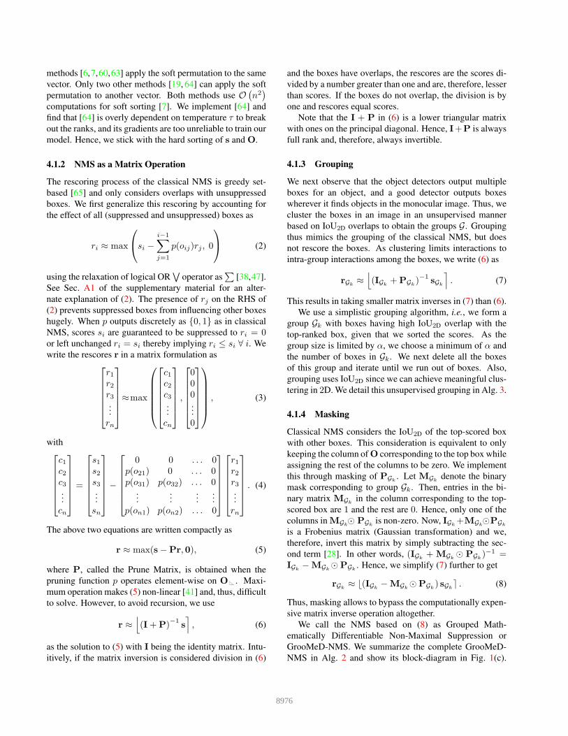
4.1.2 NMS as a Matrix Operation
The rescoring process of the classical NMS is greedy set-
based [65] and only considers overlaps with unsuppressed
boxes. We first generalize this rescoring by accounting for
the effect of all (suppressed and unsuppressed) boxes as
ri ≈ max
si −i−1∑
j=1
p(oij)rj , 0
(2)
using the relaxation of logical OR∨
operator as∑
[38,47].
See Sec. A1 of the supplementary material for an alter-
nate explanation of (2). The presence of rj on the RHS of
(2) prevents suppressed boxes from influencing other boxes
hugely. When p outputs discretely as {0, 1} as in classical
NMS, scores si are guaranteed to be suppressed to ri = 0or left unchanged ri = si thereby implying ri ≤ si ∀ i. We
write the rescores r in a matrix formulation as
r1r2r3...
rn
≈max
c1c2c3...
cn
,
000...
0
, (3)
with
c1c2c3...
cn
=
s1s2s3...
sn
−
0 0 . . . 0p(o21) 0 . . . 0p(o31) p(o32) . . . 0
......
......
p(on1) p(on2) . . . 0
r1r2r3...
rn
. (4)
The above two equations are written compactly as
r ≈ max(s−Pr,0), (5)
where P, called the Prune Matrix, is obtained when the
pruning function p operates element-wise on O❧
❧ . Maxi-
mum operation makes (5) non-linear [41] and, thus, difficult
to solve. However, to avoid recursion, we use
r ≈⌊
(I+P)−1
s
⌉
, (6)
as the solution to (5) with I being the identity matrix. Intu-
itively, if the matrix inversion is considered division in (6)
and the boxes have overlaps, the rescores are the scores di-
vided by a number greater than one and are, therefore, lesser
than scores. If the boxes do not overlap, the division is by
one and rescores equal scores.
Note that the I + P in (6) is a lower triangular matrix
with ones on the principal diagonal. Hence, I+P is always
full rank and, therefore, always invertible.
4.1.3 Grouping
We next observe that the object detectors output multiple
boxes for an object, and a good detector outputs boxes
wherever it finds objects in the monocular image. Thus, we
cluster the boxes in an image in an unsupervised manner
based on IoU2D overlaps to obtain the groups G. Grouping
thus mimics the grouping of the classical NMS, but does
not rescore the boxes. As clustering limits interactions to
intra-group interactions among the boxes, we write (6) as
rGk≈
⌊
(IGk+PGk
)−1
sGk
⌉
. (7)
This results in taking smaller matrix inverses in (7) than (6).
We use a simplistic grouping algorithm, i.e., we form a
group Gk with boxes having high IoU2D overlap with the
top-ranked box, given that we sorted the scores. As the
group size is limited by α, we choose a minimum of α and
the number of boxes in Gk. We next delete all the boxes
of this group and iterate until we run out of boxes. Also,
grouping uses IoU2D since we can achieve meaningful clus-
tering in 2D. We detail this unsupervised grouping in Alg. 3.
4.1.4 Masking
Classical NMS considers the IoU2D of the top-scored box
with other boxes. This consideration is equivalent to only
keeping the column of O corresponding to the top box while
assigning the rest of the columns to be zero. We implement
this through masking of PGk. Let MGk
denote the binary
mask corresponding to group Gk. Then, entries in the bi-
nary matrix MGkin the column corresponding to the top-
scored box are 1 and the rest are 0. Hence, only one of the
columns in MGk⊙ PGk
is non-zero. Now, IGk+MGk
⊙PGk
is a Frobenius matrix (Gaussian transformation) and we,
therefore, invert this matrix by simply subtracting the sec-
ond term [28]. In other words, (IGk+ MGk
⊙ PGk)−1 =
IGk−MGk
⊙PGk. Hence, we simplify (7) further to get
rGk≈ ⌊(IGk
−MGk⊙PGk
) sGk⌉ . (8)
Thus, masking allows to bypass the computationally expen-
sive matrix inverse operation altogether.
We call the NMS based on (8) as Grouped Math-
ematically Differentiable Non-Maximal Suppression or
GrooMeD-NMS. We summarize the complete GrooMeD-
NMS in Alg. 2 and show its block-diagram in Fig. 1(c).
8976

Figure 2: Pruning functions p of the classical and GrooMeD-
NMS. We use the Linear and Exponential pruning of the Soft-
NMS [8] while training with the GrooMeD-NMS.
GrooMeD-NMS in Fig. 1(c) provides two gradients - one
through s and other through O.
4.1.5 Pruning Function
As explained in Sec. 3.1, the pruning function p decides
whether to keep the box in the final set of predictions D or
not based on IoU2D overlaps, i.e., p(oi) = 1 denotes the box
bi is suppressed while p(oi) = 0 denotes bi is kept in D.
Classical NMS uses the threshold as the pruning func-
tion, which does not give useful gradients. Therefore, we
considered three different functions for p: Linear, a temper-
ature (τ)-controlled Exponential, and Sigmoidal function.
• Linear Linear pruning function [8] is p(o) = o.
• Exponential Exponential pruning function [8] is
p(o) = 1− exp(
− o2
τ
)
.
• Sigmoidal Sigmoidal pruning function is p(o) =σ(
o−Nt
τ
)
with σ denoting the standard sigmoid. Sig-
moidal function appears as the binary cross entropy re-
laxation of the subset selection problem [60].
We show these pruning functions in Fig. 2. The ablation
studies (Sec. 5.4) show that choosing p as Linear yields the
simplest and the best GrooMeD-NMS.
4.2. Differences from Existing NMS
Although no differentiable NMS has been proposed
for the monocular 3D object detection, we compare our
GrooMeD-NMS with the NMS proposed for 2D object de-
tection, 2D pedestrian detection, 2D salient object detec-
tion, and 3D object detection in Tab. 1. No method de-
scribed in Tab. 1 has a matrix-based closed-form mathe-
matical expression of the NMS. Classical, Soft [8] and
Distance-NMS [76] are used at the inference time, while
GrooMeD-NMS is used during both training and inference.
Distance-NMS [76] updates the z-coordinate of the box af-
ter NMS as the weighted average of the z-coordinates of
top-κ boxes. QUBO-NMS [73], Point-NMS [42, 81], and
MAP-NMS [91] are not used in end-to-end training. [3] pro-
poses a trainable Point-NMS. The Structured-SVM based
NMS [21,86] rely on structured SVM to obtain the rescores.
Table 1: Overview of different NMS. [Key: Train= End-to-end
Trainable, Prune= Pruning function, #Layers= Number of layers,
Par= Parallelizable]
NMS Train Rescore Prune #Layers Par
Classical ✕ ✕ Hard - O (|G|)Soft-NMS [8] ✕ ✕ Soft - O (|G|)Distance-NMS [76] ✕ ✕ Hard - O (|G|)QUBO-NMS [73] ✕ Optimization ✕ - -
Point-NMS [42, 81] ✕ Point Process ✕ - -
Trainable Point-NMS [3] X Point Process ✕ - -
MAP-NMS [91] ✕ MAP ✕ - -
Structured-NMS [21, 86] ✕ SSVM ✕ - -
Adaptive-NMS [51] ✕ ✕ Hard >1 O (|G|)NN-NMS [31, 32, 65] X Neural Network ✕ >1 O (1)
GrooMeD-NMS (Ours) X Matrix Soft 1 O (|G|)
Adaptive-NMS [51] uses a separate neural network to pre-
dict the classical NMS threshold Nt. The trainable neural
network based NMS (NN-NMS) [31, 32, 65] use a separate
neural network containing multiple layers and/or message-
passing to approximate the NMS and do not use the prun-
ing function. Unlike these methods, GrooMeD-NMS uses a
single layer and does not require multiple layers or message
passing. Our NMS is parallel up to group (denoted by G).
However, |G| is, in general, << |B| in the NMS.
4.3. Target Assignment and Loss Function
Target Assignment. Our method consists of M3D-
RPN [10] and uses binning and self-balancing confi-
dence [12]. The boxes’ self-balancing confidence are used
as scores s, which pass through the GrooMeD-NMS layer
to obtain the rescores r. The rescores signal the network if
the best box has not been selected for a particular object.
We extend the notion of the best 2D box [65] to 3D. The
best box has the highest product of IoU2D and gIoU3D [71]
with ground truth gl. If the product is greater than a certain
threshold β, it is assigned a positive label. Mathematically,
target(bi) =
1,if ∃ gl st i = argmax q(bj , gl)
and q(bi, gl) ≥ β
0, otherwise
(9)
with q(bj , gl) = IoU2D(bj , gl)(
1+gIoU3D(bj ,gl)2
)
. gIoU3D is
known to provide signal even for non-intersecting
boxes [71], where the usual IoU3D is always zero. There-
fore, we use gIoU3D instead of regular IoU3D for figur-
ing out the best box in 3D as many 3D boxes have a
zero IoU3D overlap with the ground truth. For calculating
gIoU3D, we first calculate the volume V and hull volume
Vhull of the 3D boxes. Vhull is the product of gIoU2D in
Birds Eye View (BEV), removing the rotations and hull of
the Y dimension. gIoU3D is then given by
gIoU3D(bi, bj) =V (bi ∩ bj)
V (bi ∪ bj)+
V (bi ∪ bj)
Vhull(bi, bj)− 1. (10)
Loss Function. Generally the number of best boxes is less
than the number of ground truths in an image, as there could
8977
be some ground truth boxes for which no box is predicted.
The tiny number of best boxes introduces a far-heavier skew
than the foreground-background classification. Thus, we
use the modified AP-Loss [14] as our loss after NMS since
AP-Loss does not suffer from class imbalance [14].
Vanilla AP-Loss treats boxes of all images in a mini-
batch equally, and the gradients are back-propagated
through all the boxes. We remove this condition and rank
boxes in an image-wise manner. In other words, if the best
boxes are correctly ranked in one image and are not in the
second, then the gradients only affect the boxes of the sec-
ond image. We call this modification of AP-Loss as Image-
wise AP-Loss. In other words,
LImagewise =1
N
N∑
m=1
AP(r(m), target(B(m))), (11)
where r(m) and B(m) denote the rescores and the boxes of
the mth image in a mini-batch respectively. This is differ-
ent from previous NMS approaches [30–32, 65], which use
classification losses. Our ablation studies (Sec. 5.4) show
that the Imagewise AP-Loss is better suited to be used after
NMS than the classification loss.
Our overall loss function is thus given by L = Lbefore+λLafter where Lbefore denotes the losses before the NMS
including classification, 2D and 3D regression as well as
confidence losses, and Lafter denotes the loss term after
the NMS, which is the Imagewise AP-Loss with λ being
the weight. See Sec. A2 of the supplementary material for
more details of the loss function.
5. Experiments
Our experiments use the most widely used KITTI au-
tonomous driving dataset [25]. We modify the publicly-
available PyTorch [59] code of Kinematic-3D [12]. [12]
uses DenseNet-121 [34] trained on ImageNet as the back-
bone and nh = 1,024 using 3D-RPN settings of [10]. As
[12] is a video-based method while GrooMeD-NMS is an
image-based method, we use the best image model of [12]
henceforth called Kinematic (Image) as our baseline for
a fair comparison. Kinematic (Image) is built on M3D-
RPN [10] and uses binning and self-balancing confidence.
Data Splits. There are three commonly used data splits of
the KITTI dataset; we evaluate our method on all three.
Test Split: Official KITTI 3D benchmark [1] consists of
7,481 training and 7,518 testing images [25].
Val 1 Split: It partitions the 7,481 training images into
3,712 training and 3,769 validation images [12, 16, 77].
Val 2 Split: It partitions the 7,481 training images into
3,682 training and 3,799 validation images [89].
Training. Training is done in two phases - warmup and
full [12]. We initialize the model with the confidence pre-
diction branch from warmup weights and finetune using the
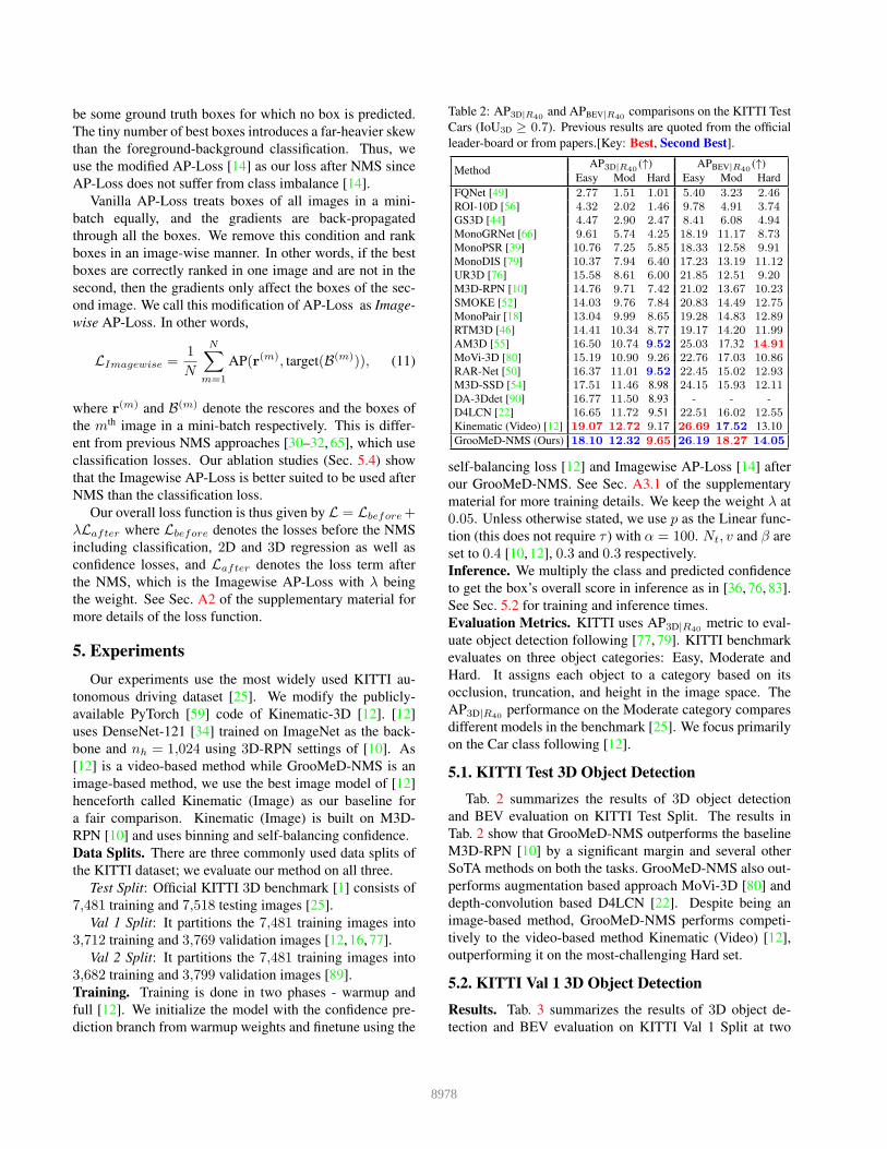
Table 2: AP3D|R40and APBEV|R40
comparisons on the KITTI Test
Cars (IoU3D ≥ 0.7). Previous results are quoted from the official
leader-board or from papers.[Key: Best, Second Best].
MethodAP3D|R40
(↑) APBEV|R40(↑)
Easy Mod Hard Easy Mod Hard
FQNet [49] 2.77 1.51 1.01 5.40 3.23 2.46ROI-10D [56] 4.32 2.02 1.46 9.78 4.91 3.74GS3D [44] 4.47 2.90 2.47 8.41 6.08 4.94MonoGRNet [66] 9.61 5.74 4.25 18.19 11.17 8.73MonoPSR [39] 10.76 7.25 5.85 18.33 12.58 9.91MonoDIS [79] 10.37 7.94 6.40 17.23 13.19 11.12UR3D [76] 15.58 8.61 6.00 21.85 12.51 9.20M3D-RPN [10] 14.76 9.71 7.42 21.02 13.67 10.23SMOKE [52] 14.03 9.76 7.84 20.83 14.49 12.75MonoPair [18] 13.04 9.99 8.65 19.28 14.83 12.89RTM3D [46] 14.41 10.34 8.77 19.17 14.20 11.99AM3D [55] 16.50 10.74 9.52 25.03 17.32 14.91
MoVi-3D [80] 15.19 10.90 9.26 22.76 17.03 10.86RAR-Net [50] 16.37 11.01 9.52 22.45 15.02 12.93M3D-SSD [54] 17.51 11.46 8.98 24.15 15.93 12.11DA-3Ddet [90] 16.77 11.50 8.93 - - -
D4LCN [22] 16.65 11.72 9.51 22.51 16.02 12.55Kinematic (Video) [12] 19.07 12.72 9.17 26.69 17.52 13.10
GrooMeD-NMS (Ours) 18.10 12.32 9.65 26.19 18.27 14.05
self-balancing loss [12] and Imagewise AP-Loss [14] after
our GrooMeD-NMS. See Sec. A3.1 of the supplementary
material for more training details. We keep the weight λ at
0.05. Unless otherwise stated, we use p as the Linear func-
tion (this does not require τ ) with α = 100. Nt, v and β are
set to 0.4 [10, 12], 0.3 and 0.3 respectively.
Inference. We multiply the class and predicted confidence
to get the box’s overall score in inference as in [36, 76, 83].
See Sec. 5.2 for training and inference times.
Evaluation Metrics. KITTI uses AP3D|R40metric to eval-
uate object detection following [77, 79]. KITTI benchmark
evaluates on three object categories: Easy, Moderate and
Hard. It assigns each object to a category based on its
occlusion, truncation, and height in the image space. The
AP3D|R40performance on the Moderate category compares
different models in the benchmark [25]. We focus primarily
on the Car class following [12].
5.1. KITTI Test 3D Object Detection
Tab. 2 summarizes the results of 3D object detection
and BEV evaluation on KITTI Test Split. The results in
Tab. 2 show that GrooMeD-NMS outperforms the baseline
M3D-RPN [10] by a significant margin and several other
SoTA methods on both the tasks. GrooMeD-NMS also out-
performs augmentation based approach MoVi-3D [80] and
depth-convolution based D4LCN [22]. Despite being an
image-based method, GrooMeD-NMS performs competi-
tively to the video-based method Kinematic (Video) [12],
outperforming it on the most-challenging Hard set.
5.2. KITTI Val 1 3D Object Detection
Results. Tab. 3 summarizes the results of 3D object de-
tection and BEV evaluation on KITTI Val 1 Split at two
8978

Table 3: AP3D|R40and APBEV|R40
comparisons on KITTI Val 1 Cars. [Key: Best, Second Best].
Method
IoU3D ≥ 0.7 IoU3D ≥ 0.5AP3D|R40
(↑) APBEV|R40(↑) AP3D|R40
(↑) APBEV|R40(↑)
Easy Mod Hard Easy Mod Hard Easy Mod Hard Easy Mod Hard
MonoDR [5] 12.50 7.34 4.98 19.49 11.51 8.72 - - - - - -
MonoGRNet [66] in [18] 11.90 7.56 5.76 19.72 12.81 10.15 47.59 32.28 25.50 52.13 35.99 28.72MonoDIS [79] in [77] 11.06 7.60 6.37 18.45 12.58 10.66 - - - - - -
M3D-RPN [10] in [12] 14.53 11.07 8.65 20.85 15.62 11.88 48.56 35.94 28.59 53.35 39.60 31.77MoVi-3D [80] 14.28 11.13 9.68 22.36 17.87 15.73 - - - - - -
MonoPair [18] 16.28 12.30 10.42 24.12 18.17 15.76 55.38 42.39 37.99 61.06 47.63 41.92
Kinematic (Image) [12] 18.28 13.55 10.13 25.72 18.82 14.48 54.70 39.33 31.25 60.87 44.36 34.48Kinematic (Video) [12] 19.76 14.10 10.47 27.83 19.72 15.10 55.44 39.47 31.26 61.79 44.68 34.56GrooMeD-NMS (Ours) 19.67 14.32 11.27 27.38 19.75 15.92 55.62 41.07 32.89 61.83 44.98 36.29
Table 4: AP3D|R40and APBEV|R40
comparisons with other NMS
on KITTI Val 1 Cars (IoU3D ≥ 0.7). [Key: C= Classical, S= Soft-
NMS [8], D= Distance-NMS [76], G= GrooMeD-NMS]
MethodInferNMS
AP3D|R40(↑) APBEV|R40
(↑)
Easy Mod Hard Easy Mod Hard
Kinematic (Image) C 18.28 13.55 10.13 25.72 18.82 14.48Kinematic (Image) S 18.29 13.55 10.13 25.71 18.81 14.48Kinematic (Image) D 18.25 13.53 10.11 25.71 18.82 14.48Kinematic (Image) G 18.26 13.51 10.10 25.67 18.77 14.44GrooMeD-NMS C 19.67 14.31 11.27 27.38 19.75 15.93GrooMeD-NMS S 19.67 14.31 11.27 27.38 19.75 15.93GrooMeD-NMS D 19.67 14.31 11.27 27.38 19.75 15.93GrooMeD-NMS G 19.67 14.32 11.27 27.38 19.75 15.92
(a) Linear Scale (b) Log Scale
Figure 3: Comparison of AP3D at different depths and
IoU3D matching thresholds on KITTI Val 1 Split.
IoU3D thresholds of 0.7 and 0.5 [12, 18]. The results in
Tab. 3 show that GrooMeD-NMS outperforms the baseline
of M3D-RPN [10] and Kinematic (Image) [12] by a sig-
nificant margin. Interestingly, GrooMeD-NMS (an image-
based method) also outperforms the video-based method
Kinematic (Video) [12] on most of the metrics. Thus,
GrooMeD-NMS performs best on 6 out of the 12 cases (3categories × 2 tasks × 2 thresholds) while second-best on
all other cases. The performance is especially impressive
since the biggest improvements are shown on the Moderate
and Hard set, where objects are more distant and occluded.
AP3D at different depths and IoU3D thresholds. We next
compare the AP3D performance of GrooMeD-NMS and
Kinematic (Image) on linear and log scale for objects at dif-
ferent depths of [15, 30, 45, 60] meters and IoU3D match-
ing criteria of 0.3 −� 0.7 in Fig. 3 as in [12]. Fig. 3
shows that GrooMeD-NMS outperforms the Kinematic
(Image) [12] at all depths and all IoU3D thresholds.
Comparisons with other NMS. We compare with the clas-
Figure 4: Score-IoU3D plot after the NMS.
sical NMS, Soft-NMS [8] and Distance-NMS [76] in Tab. 4.
More detailed results are in Tab. 8 of the supplementary ma-
terial. The results show that NMS inclusion in the train-
ing pipeline benefits the performance, unlike [8], which
suggests otherwise. Training with GrooMeD-NMS helps
because the network gets an additional signal through the
GrooMeD-NMS layer whenever the best-localized box cor-
responding to an object is not selected. Interestingly, Tab. 4
also suggests that replacing GrooMeD-NMS with the clas-
sical NMS in inference does not affect the performance.
Score-IoU3D Plot. We further correlate the scores with
IoU3D after NMS of our model with two baselines - M3D-
RPN [10] and Kinematic (Image) [12] and also the Kine-
matic (Video) [12] in Fig. 4. We obtain the best correlation
of 0.345 exceeding the correlations of M3D-RPN, Kine-
matic (Image) and, also Kinematic (Video). This proves
that including NMS in the training pipeline is beneficial.
Training and Inference Times. We now compare the train-
ing and inference times of including GrooMeD-NMS in
the pipeline. Warmup training phase takes about 13 hours
to train on a single 12 GB GeForce GTX Titan-X GPU.
Full training phase of Kinematic (Image) and GrooMeD-
NMS takes about 8 and 8.5 hours respectively. The infer-
ence time per image using classical and GrooMeD-NMS is
0.12 and 0.15 ms respectively. Tab. 4 suggests that chang-
ing the NMS from GrooMeD to classical during inference
does not alter the performance. Then, the inference time of
our method is the same as 0.12 ms.
5.3. KITTI Val 2 3D Object Detection
Tab. 5 summarizes the results of 3D object detection and
BEV evaluation on KITTI Val 2 Split at two IoU3D thresh-
8979
Table 5: AP3D|R40and APBEV|R40
comparisons on KITTI Val 2 Cars. [Key: Best, *= Released, †= Retrained].
Method
IoU3D ≥ 0.7 IoU3D ≥ 0.5AP3D|R40
(↑) APBEV|R40(↑) AP3D|R40
(↑) APBEV|R40(↑)
Easy Mod Hard Easy Mod Hard Easy Mod Hard Easy Mod Hard
M3D-RPN [10]* 14.57 10.07 7.51 21.36 15.22 11.28 49.14 34.43 26.39 53.44 37.79 29.36Kinematic (Image) [12]† 13.54 10.21 7.24 20.60 15.14 11.30 51.53 36.55 28.26 56.20 40.02 31.25GrooMeD-NMS (Ours) 14.72 10.87 7.67 22.03 16.05 11.93 51.91 36.78 28.40 56.29 40.31 31.39
Table 6: Ablation studies of our method on KITTI Val 1 Cars.
Change from GrooMeD-NMS model: IoU3D ≥ 0.7 IoU3D ≥ 0.5
Changed From −−�ToAP3D|R40
(↑) APBEV|R40(↑) AP3D|R40
(↑) APBEV|R40(↑)
Easy Mod Hard Easy Mod Hard Easy Mod Hard Easy Mod Hard
Training
Conf+NMS−�No Conf+No NMS 16.66 12.10 9.40 23.15 17.43 13.48 51.47 38.58 30.98 56.48 42.53 34.37Conf+NMS−�Conf+No NMS 19.16 13.89 10.96 27.01 19.33 14.84 57.12 41.07 32.79 61.60 44.58 35.97Conf+NMS−�No Conf+NMS 15.02 11.21 8.83 21.07 16.27 12.77 48.01 36.18 29.96 53.82 40.94 33.35
Initialization No Warmup 15.33 11.68 8.78 21.32 16.59 12.93 49.15 37.42 30.11 54.32 41.44 33.48
Pruning
Function
Linear−�Exponential, τ = 1 12.81 9.26 7.10 17.07 12.17 9.25 29.58 20.42 15.88 32.06 22.16 17.20Linear−�Exponential, τ = 0.5 [8] 18.63 13.85 10.98 27.52 20.14 15.76 56.64 41.01 32.79 61.43 44.73 36.02Linear−�Exponential, τ = 0.1 18.34 13.79 10.88 27.26 19.71 15.90 56.98 41.16 32.96 62.77 45.23 36.56Linear−�Sigmoidal, τ = 0.1 17.40 13.21 9.80 26.77 19.26 14.76 55.15 40.77 32.63 60.56 44.23 35.74
Group+MaskGroup+Mask−�No Group 18.43 13.91 11.08 26.53 19.46 15.83 55.93 40.98 32.78 61.02 44.77 36.09Group+Mask−�Group+No Mask 18.99 13.74 10.24 26.71 19.21 14.77 55.21 40.69 32.55 61.74 44.67 36.00
LossImagewise AP−�Vanilla AP 18.23 13.73 10.28 26.42 19.31 14.76 54.47 40.35 32.20 60.90 44.08 35.47Imagewise AP−�BCE 16.34 12.74 9.73 22.40 17.46 13.70 52.46 39.40 31.68 58.22 43.60 35.27
Inference Class*Pred−�Class 18.26 13.36 10.49 25.39 18.64 15.12 52.44 38.99 31.3 57.37 42.89 34.68NMS Scores Class*Pred−�Pred 17.51 12.84 9.55 24.55 17.85 13.63 52.78 37.48 29.37 58.30 41.26 32.66
— GrooMeD-NMS (best model) 19.67 14.32 11.27 27.38 19.75 15.92 55.62 41.07 32.89 61.83 44.98 36.29
olds of 0.7 and 0.5 [12, 18]. Again, we use M3D-RPN [10]
and Kinematic (Image) [12] as our baselines. We evaluate
the released model of M3D-RPN [10] using the KITTI met-
ric. [12] does not report Val 2 results, so we retrain on Val
2 using their public code. The results in Tab. 5 show that
GrooMeD-NMS performs best in all cases. This is again
impressive because the improvements are shown on Moder-
ate and Hard set, consistent with Tabs. 2 and 3.
5.4. Ablation Studies
Tab. 6 compares the modifications of our approach on
KITTI Val 1 Cars. Unless stated otherwise, we stick with
the experimental settings described in Sec. 5. Using a
confidence head (Conf+No NMS) proves beneficial com-
pared to the warmup model (No Conf+No NMS), which
is consistent with the observations of [12, 76]. Further,
GrooMeD-NMS on classification scores (denoted by No
Conf + NMS) is detrimental as the classification scores are
not suited for localization [12, 35]. Training the warmup
model and then finetuning also works better than training
without warmup as in [12] since the warmup phase allows
GrooMeD-NMS to carry meaningful grouping of the boxes.
As described in Sec. 4.1.5, in addition to Linear, we com-
pare two other functions for pruning function p: Exponen-
tial and Sigmoidal. Both of them do not perform as well
as the Linear p possibly because they have vanishing gradi-
ents close to overlap of zero or one. Grouping and masking
both help our model to reach a better minimum. As de-
scribed in Sec. 4.3, Imagewise AP loss is better than the
Vanilla AP loss since it treats boxes of two images differ-
ently. Imagewise AP also performs better than the binary
cross-entropy (BCE) loss proposed in [30–32, 65]. Using
the product of self-balancing confidence and classification
scores instead of using them individually as the scores to
the NMS in inference is better, consistent with [36, 76, 83].
Class confidence performs worse since it does not have
the localization information while the self-balancing con-
fidence (Pred) gives the localization without considering
whether the box belongs to foreground or background.
6. Conclusions
In this paper, we present and integrate GrooMeD-NMS –
a novel Grouped Mathematically Differentiable NMS for
monocular 3D object detection, such that the network is
trained end-to-end with a loss on the boxes after NMS. We
first formulate NMS as a matrix operation and then do un-
supervised grouping and masking of the boxes to obtain
a simple closed-form expression of the NMS. GrooMeD-
NMS addresses the mismatch between training and infer-
ence pipelines and, therefore, forces the network to se-
lect the best 3D box in a differentiable manner. As a
result, GrooMeD-NMS achieves state-of-the-art monoc-
ular 3D object detection results on the KITTI bench-
mark dataset. Although our implementation demonstrates
monocular 3D object detection, GrooMeD-NMS is fairly
generic for other object detection tasks. Future work in-
cludes applying this method to tasks such as LiDAR-based
3D object detection and pedestrian detection.
8980

References
[1] The KITTI Vision Benchmark Suite. http://www.
cvlibs.net/datasets/kitti/eval_object.
php?obj_benchmark=3d. Accessed: 2020-10-11. 6
[2] Hassan Alhaija, Siva Mustikovela, Lars Mescheder, Andreas
Geiger, and Carsten Rother. Augmented reality meets com-
puter vision: Efficient data generation for urban driving
scenes. IJCV, 2018. 1
[3] Samaneh Azadi, Jiashi Feng, and Trevor Darrell. Learning
detection with diverse proposals. In CVPR, 2017. 2, 5
[4] Wentao Bao, Bin Xu, and Zhenzhong Chen. MonoFENet:
Monocular 3D object detection with feature enhancement
networks. IEEE Transactions on Image Processing, 2019.
2
[5] Deniz Beker, Hiroharu Kato, Mihai Adrian Morariu,
Takahiro Ando, Toru Matsuoka, Wadim Kehl, and Adrien
Gaidon. Monocular differentiable rendering for self-
supervised 3D object detection. In ECCV, 2020. 7
[6] Quentin Berthet, Mathieu Blondel, Olivier Teboul, Marco
Cuturi, Jean-Philippe Vert, and Francis Bach. Learning with
differentiable perturbed optimizers. In NeurIPS, 2020. 4
[7] Mathieu Blondel, Olivier Teboul, Quentin Berthet, and Josip
Djolonga. Fast differentiable sorting and ranking. In ICML,
2020. 4
[8] Navaneeth Bodla, Bharat Singh, Rama Chellappa, and Larry
Davis. Soft-NMS–improving object detection with one line
of code. In ICCV, 2017. 2, 3, 5, 7, 8, 14
[9] Navaneeth Bodla, Bharat Singh, Rama Chellappa, and Larry
Davis. Soft-NMS implementation. https://github.
com/bharatsingh430/soft-nms/blob/master/
lib/nms/cpu_nms.pyx#L98, 2017. Accessed: 2021-
01-18. 3
[10] Garrick Brazil and Xiaoming Liu. M3D-RPN: Monocular
3D region proposal network for object detection. In ICCV,
2019. 1, 2, 5, 6, 7, 8, 13, 14
[11] Garrick Brazil and Xiaoming Liu. Pedestrian detection with
autoregressive network phases. In CVPR, 2019. 2
[12] Garrick Brazil, Gerard Pons-Moll, Xiaoming Liu, and Bernt
Schiele. Kinematic 3D object detection in monocular video.
In ECCV, 2020. 1, 2, 5, 6, 7, 8, 13, 14, 15, 16
[13] Garrick Brazil, Xi Yin, and Xiaoming Liu. Illuminating
pedestrians via simultaneous detection & segmentation. In
ICCV, 2017. 2
[14] Kean Chen, Weiyao Lin, Jianguo Li, John See, Ji Wang, and
Junni Zou. AP-Loss for accurate one-stage object detection.
TPAMI, 2020. 6
[15] Xiaozhi Chen, Kaustav Kundu, Ziyu Zhang, Huimin Ma,
Sanja Fidler, and Raquel Urtasun. Monocular 3D object de-
tection for autonomous driving. In CVPR, 2016. 2
[16] Xiaozhi Chen, Kaustav Kundu, Yukun Zhu, Andrew Berne-
shawi, Huimin Ma, Sanja Fidler, and Raquel Urtasun. 3D
object proposals for accurate object class detection. In
NeurIPS, 2015. 6
[17] Xiaozhi Chen, Huimin Ma, Ji Wan, Bo Li, and Tian Xia.
Multi-view 3D object detection network for autonomous
driving. In CVPR, 2017. 1, 2
[18] Yongjian Chen, Lei Tai, Kai Sun, and Mingyang Li.
MonoPair: Monocular 3D object detection using pairwise
spatial relationships. In CVPR, 2020. 1, 2, 6, 7, 8
[19] Marco Cuturi, Olivier Teboul, and Jean-Philippe Vert. Dif-
ferentiable ranks and sorting using optimal transport. In
NeurIPS, 2019. 4
[20] Navneet Dalal and Bill Triggs. Histograms of oriented gra-
dients for human detection. In CVPR, 2005. 2
[21] Chaitanya Desai, Deva Ramanan, and Charless Fowlkes.
Discriminative models for multi-class object layout. IJCV,
2011. 2, 5
[22] Mingyu Ding, Yuqi Huo, Hongwei Yi, Zhe Wang, Jianping
Shi, Zhiwu Lu, and Ping Luo. Learning depth-guided convo-
lutions for monocular 3D object detection. In CVPR Work-
shops, 2020. 2, 6
[23] Sanja Fidler, Sven Dickinson, and Raquel Urtasun. 3D ob-
ject detection and viewpoint estimation with a deformable
3D cuboid model. In NeurIPS, 2012. 2
[24] Andreas Geiger, Philip Lenz, Christoph Stiller, and Raquel
Urtasun. Vision meets robotics: The KITTI dataset. IJRR,
2013. 15
[25] Andreas Geiger, Philip Lenz, and Raquel Urtasun. Are we
ready for autonomous driving? the KITTI vision benchmark
suite. In CVPR, 2012. 6
[26] Ross Girshick. Fast R-CNN. In ICCV, 2015. 2
[27] Ross Girshick, Jeff Donahue, Trevor Darrell, and Jitendra
Malik. Rich feature hierarchies for accurate object detection
and semantic segmentation. In CVPR, 2014. 2
[28] Gene Golub and Charles Loan. Matrix computations. 2013.
4
[29] Christopher Harris and Mike Stephens. A combined corner
and edge detector. In Alvey vision conference, 1988. 2
[30] Paul Henderson and Vittorio Ferrari. End-to-end training of
object class detectors for mean average precision. In ACCV,
2016. 2, 6, 8
[31] Jan Hosang, Rodrigo Benenson, and Bernt Schiele. A con-
vnet for non-maximum suppression. In GCPR, 2016. 2, 5,
6, 8
[32] Jan Hosang, Rodrigo Benenson, and Bernt Schiele. Learning
non-maximum suppression. In CVPR, 2017. 2, 5, 6, 8, 15
[33] Peiyun Hu, Jason Ziglar, David Held, and Deva Ramanan.
What you see is what you get: Exploiting visibility for 3D
object detection. In CVPR, 2020. 2
[34] Gao Huang, Zhuang Liu, Laurens Maaten, and Kilian Wein-
berger. Densely connected convolutional networks. In
CVPR, 2017. 6
[35] Tengteng Huang, Zhe Liu, Xiwu Chen, and Xiang Bai. EP-
Net: Enhancing point features with image semantics for 3D
object detection. In ECCV, 2020. 1, 2, 8
[36] Kang Kim and Hee Lee. Probabilistic anchor assignment
with iou prediction for object detection. In ECCV, 2020. 6,
8
[37] Diederik Kingma and Jimmy Ba. Adam: A method for
stochastic optimization. In ICLR, 2015. 13
[38] Emile Krieken, Erman Acar, and Frank Harmelen. Ana-
lyzing differentiable fuzzy logic operators. arXiv preprint
arXiv:2002.06100, 2020. 4, 12
8981
[39] Jason Ku, Alex Pon, and Steven Waslander. Monocular 3D
object detection leveraging accurate proposals and shape re-
construction. In CVPR, 2019. 6
[40] Abhinav Kumar, Tim Marks, Wenxuan Mou, Ye Wang,
Michael Jones, Anoop Cherian, Toshiaki Koike-Akino, Xi-
aoming Liu, and Chen Feng. LUVLi face alignment: Esti-
mating landmarks’ location, uncertainty, and visibility like-
lihood. In CVPR, 2020. 2
[41] Animesh Kumar and Vinod Prabhakaran. Estimation of ban-
dlimited signals from the signs of noisy samples. In ICASSP,
2013. 4, 13
[42] Donghoon Lee, Geonho Cha, Ming-Hsuan Yang, and Songh-
wai Oh. Individualness and determinantal point processes for
pedestrian detection. In ECCV, 2016. 2, 5
[43] Sergey Levine, Peter Pastor, Alex Krizhevsky, Julian Ibarz,
and Deirdre Quillen. Learning hand-eye coordination for
robotic grasping with deep learning and large-scale data col-
lection. IJRR, 2018. 1
[44] Buyu Li, Wanli Ouyang, Lu Sheng, Xingyu Zeng, and Xiao-
gang Wang. GS3D: An efficient 3D object detection frame-
work for autonomous driving. In CVPR, 2019. 1, 6
[45] Peiliang Li, Xiaozhi Chen, and Shaojie Shen. Stereo R-CNN
based 3D object detection for autonomous driving. In CVPR,
2019. 2
[46] Peixuan Li, Huaici Zhao, Pengfei Liu, and Feidao Cao.
RTM3D: Real-time monocular 3D detection from object
keypoints for autonomous driving. In ECCV, 2020. 1, 2,
6
[47] Tao Li and Vivek Srikumar. Augmenting neural networks
with first-order logic. In ACL, 2019. 4, 12
[48] Tsung-Yi Lin, Priya Goyal, Ross Girshick, Kaiming He, and
Piotr Dollar. Focal loss for dense object detection. TPAMI,
2018. 2
[49] Lijie Liu, Jiwen Lu, Chunjing Xu, Qi Tian, and Jie Zhou.
Deep fitting degree scoring network for monocular 3D object
detection. In CVPR, 2019. 2, 6
[50] Lijie Liu, Chufan Wu, Jiwen Lu, Lingxi Xie, Jie Zhou, and
Qi Tian. Reinforced axial refinement network for monocular
3D object detection. In ECCV, 2020. 6
[51] Songtao Liu, Di Huang, and Yunhong Wang. Adaptive NMS:
Refining pedestrian detection in a crowd. In CVPR, 2019. 2,
5
[52] Zechen Liu, Zizhang Wu, and Roland Toth. SMOKE:
Single-stage monocular 3D object detection via keypoint es-
timation. In CVPR Workshops, 2020. 6
[53] David Lowe. Distinctive image features from scale-invariant
keypoints. IJCV, 2004. 2
[54] Shujie Luo, Hang Dai, Ling Shao, and Yong Ding.
M3DSSD: Monocular 3D single stage object detector. In
CVPR, 2021. 6
[55] Xinzhu Ma, Zhihui Wang, Haojie Li, Pengbo Zhang, Wanli
Ouyang, and Xin Fan. Accurate monocular 3D object detec-
tion via color-embedded 3D reconstruction for autonomous
driving. In ICCV, 2019. 6
[56] Fabian Manhardt, Wadim Kehl, and Adrien Gaidon. Roi-
10D: Monocular lifting of 2D detection to 6 pose and metric
shape. In CVPR, 2019. 6
[57] Krystian Mikolajczyk and Cordelia Schmid. Scale & affine
invariant interest point detectors. IJCV, 2004. 2
[58] Frank Moosmann, Oliver Pink, and Christoph Stiller. Seg-
mentation of 3D LiDAR data in non-flat urban environments
using a local convexity criterion. In Intelligent Vehicles Sym-
posium, 2009. 2
[59] Adam Paszke, Sam Gross, Francisco Massa, Adam Lerer,
James Bradbury, Gregory Chanan, Trevor Killeen, Zeming
Lin, Natalia Gimelshein, Luca Antiga, Alban Desmaison,
Andreas Kopf, Edward Yang, Zachary DeVito, Martin Rai-
son, Alykhan Tejani, Sasank Chilamkurthy, Benoit Steiner,
Lu Fang, Junjie Bai, and Soumith Chintala. PyTorch: An
imperative style, high-performance deep learning library. In
NeurIPS, 2019. 6
[60] Max Paulus, Dami Choi, Daniel Tarlow, Andreas Krause,
and Chris Maddison. Gradient estimation with stochastic
softmax tricks. In NeurIPS, 2020. 4, 5
[61] Nadia Payet and Sinisa Todorovic. From contours to 3D ob-
ject detection and pose estimation. In ICCV, 2011. 2
[62] Bojan Pepik, Michael Stark, Peter Gehler, and Bernt Schiele.
Multi-view and 3D deformable part models. TPAMI, 2015.
2
[63] Marin Pogancic, Anselm Paulus, Vit Musil, Georg Martius,
and Michal Rolinek. Differentiation of blackbox combinato-
rial solvers. In ICLR, 2019. 4
[64] Sebastian Prillo and Julian Eisenschlos. Softsort: A contin-
uous relaxation for the argsort operator. In ICML, 2020. 4
[65] Sergey Prokudin, Daniel Kappler, Sebastian Nowozin, and
Peter Gehler. Learning to filter object detections. In GCPR,
2017. 1, 2, 3, 4, 5, 6, 8, 12
[66] Zengyi Qin, Jinglu Wang, and Yan Lu. MonoGRNet: A
geometric reasoning network for 3D object localization. In
AAAI, 2019. 6, 7
[67] Joseph Redmon, Santosh Divvala, Ross Girshick, and Ali
Farhadi. You only look once: Unified, real-time object de-
tection. In CVPR, 2016. 2
[68] Konstantinos Rematas, Ira Kemelmacher-Shlizerman, Brian
Curless, and Steve Seitz. Soccer on your tabletop. In CVPR,
2018. 1
[69] Shaoqing Ren, Kaiming He, Ross Girshick, and Jian Sun.
Faster R-CNN: Towards real-time object detection with re-
gion proposal networks. In NeurIPS, 2015. 1, 2
[70] David Rey, Gerard Subsol, Herve Delingette, and Nicholas
Ayache. Automatic detection and segmentation of evolv-
ing processes in 3D medical images: Application to multiple
sclerosis. Medical Image Analysis, 2002. 1
[71] Hamid Rezatofighi, Nathan Tsoi, JunYoung Gwak, Amir
Sadeghian, Ian Reid, and Silvio Savarese. Generalized in-
tersection over union: A metric and a loss for bounding box
regression. In CVPR, 2019. 5
[72] Azriel Rosenfeld and Mark Thurston. Edge and curve detec-
tion for visual scene analysis. IEEE Transactions on Com-
puters, 1971. 2
[73] Sitapa Rujikietgumjorn and Robert Collins. Optimized
pedestrian detection for multiple and occluded people. In
CVPR, 2013. 2, 5
8982

[74] Ashutosh Saxena, Justin Driemeyer, and Andrew Ng.
Robotic grasping of novel objects using vision. IJRR, 2008.
1
[75] Shaoshuai Shi, Xiaogang Wang, and Hongsheng Li. PointR-
CNN: 3D object proposal generation and detection from
point cloud. In CVPR, 2019. 2
[76] Xuepeng Shi, Zhixiang Chen, and Tae-Kyun Kim. Distance-
normalized unified representation for monocular 3D object
detection. In ECCV, 2020. 1, 2, 5, 6, 7, 8, 14, 15
[77] Andrea Simonelli, Samuel Bulo, Lorenzo Porzi, Manuel An-
tequera, and Peter Kontschieder. Disentangling monocular
3D object detection: From single to multi-class recognition.
TPAMI, 2020. 1, 2, 6, 7
[78] Andrea Simonelli, Samuel Bulo, Lorenzo Porzi, Peter
Kontschieder, and Elisa Ricci. Demystifying pseudo-
LiDAR for monocular 3D object detection. arXiv preprint
arXiv:2012.05796, 2020. 14
[79] Andrea Simonelli, Samuel Bulo, Lorenzo Porzi, Manuel
Lopez-Antequera, and Peter Kontschieder. Disentangling
monocular 3D object detection. In ICCV, 2019. 2, 6, 7
[80] Andrea Simonelli, Samuel Bulo, Lorenzo Porzi, Elisa Ricci,
and Peter Kontschieder. Towards generalization across depth
for monocular 3D object detection. In ECCV, 2020. 2, 6, 7
[81] Samik Some, Mithun Das Gupta, and Vinay Namboodiri.
Determinantal point process as an alternative to NMS. In
BMVC, 2020. 2, 5
[82] Yunlei Tang, Sebastian Dorn, and Chiragkumar Savani.
Center3D: Center-based monocular 3D object detection with
joint depth understanding. arXiv preprint arXiv:2005.13423,
2020. 2
[83] Lachlan Tychsen-Smith and Lars Petersson. Improving ob-
ject localization with fitness NMS and bounded IoU loss. In
CVPR, 2018. 6, 8
[84] Alexandru Vasile and Richard Marino. Pose-independent au-
tomatic target detection and recognition using 3D laser radar
imagery. Lincoln laboratory journal, 2005. 2
[85] Paul Viola and Michael Jones. Rapid object detection using
a boosted cascade of simple features. In CVPR, 2001. 2
[86] Li Wan, David Eigen, and Rob Fergus. End-to-end integra-
tion of a convolution network, deformable parts model and
non-maximum suppression. In CVPR, 2015. 2, 5
[87] Yan Wang, Wei-Lun Chao, Divyansh Garg, Bharath Hariha-
ran, Mark Campbell, and Kilian Weinberger. Pseudo-LiDAR
from visual depth estimation: Bridging the gap in 3D object
detection for autonomous driving. In CVPR, 2019. 2
[88] Pengxiang Wu, Siheng Chen, and Dimitris Metaxas. Motion-
Net: Joint perception and motion prediction for autonomous
driving based on bird’s eye view maps. In CVPR, 2020. 2
[89] Yu Xiang, Wongun Choi, Yuanqing Lin, and Silvio Savarese.
Subcategory-aware convolutional neural networks for object
proposals and detection. In WACV, 2017. 6
[90] Xiaoqing Ye, Liang Du, Yifeng Shi, Yingying Li, Xiao Tan,
Jianfeng Feng, Errui Ding, and Shilei Wen. Monocular 3D
object detection via feature domain adaptation. In ECCV,
2020. 6
[91] Jianming Zhang, Stan Sclaroff, Zhe Lin, Xiaohui Shen,
Brian Price, and Radomir Mech. Unconstrained salient ob-
ject detection via proposal subset optimization. In CVPR,
2016. 2, 5
8983


![NMS Contin - [Product Monograph Template - Standard]](https://static.fdokumen.com/doc/165x107/6331e9c2ac2998afa709f15b/nms-contin-product-monograph-template-standard.jpg)