A Global Optimization Method, �BB, forGeneral Twice-Di�erentiable ConstrainedNLPs: II { Implementation andComputational ResultsC.S. Adjiman, I.P. Androulakis, and C.A. Floudas1Department of Chemical EngineeringPrinceton UniversityPrinceton, NJ 08544-5263AbstractPart I of this paper (Adjiman et al., 1997) described the theoretical foundations ofa global optimization algorithm, the �BB algorithm, which can be used to solveproblems belonging to the broad class of twice-di�erentiable NPLs. For any suchproblem, the ability to automatically generate progressively tighter convex lowerbounding problems at each iteration guarantees the convergence of the branch-and-bound �BB algorithm to within � of the global optimum solution. Severalmethods were presented for the construction of convex valid underestimators forgeneral nonconvex functions. In this second part, the performance of the proposedalgorithm and its alternative underestimators is studied through their applicationto a variety of problems. An implementation of the �BB is described and a num-ber of rules for branching variable selection and variable bound updates are shownto enhance convergence rates. A user-friendly parser facilitates problem input andprovides exibility in the selection of an underestimating strategy. In addition,the package features both automatic di�erentiation and interval arithmetic capa-bilities. Making use of all the available options, the �BB algorithm successfullyidenti�es the global optimum solution of small literature problems, of small andmedium size chemical engineering problems in the areas of reactor network design,heat exchanger network design, reactor-separator network design, of generalizedgeometric programming problems for design and control, and of batch processdesign problems with uncertainty.1Author to whom all correspondence should be addressed.1

1 IntroductionIn the �rst part of this paper, Adjiman et al. (1997) presented an optimiza-tion algorithm, the �BB algorithm, whose theoretical properties guaranteeconvergence to the global optimum solution of twice-di�erentiable NLPs ofthe form minx f(x)s:t: g(x) � 0h(x) = 0x 2 X � <n (1)where f , g and h belong to C2, the set of functions with continuous second-order derivatives, and x is a vector of size n.The �BB algorithm is based on a branch-and-bound approach, wherea lower bound on the optimal solution is obtained at each node throughthe automatic generation of a valid convex underestimating problem. If thefunctions contain any bilinear, trilinear, fractional, fractional trilinear or uni-variate concave terms, these may be underestimated through their convex en-velope. A valid convex underestimator Lnt(x) for a general nonconvex termnt(x) is constructed by subtracting a su�ciently large positive quadraticterm from nt(x):Lnt(x) = nt(x)� nXi=1 �i(xUi � xi)(xi � xLi ): (2)A necessary and su�cient condition for the convexity of Lnt(x) is the positivesemide�niteness of its Hessian matrix given by Hnt(x) + 2diag(�i). Hnt(x)is the Hessian matrix of nt(x).Several methods were presented for the rigorous computation of a validdiagonal shift matrix � = diag(�i) satisfying the convexity condition. Allprocedures require the use of interval analysis to obtain an interval Hessianmatrix or an interval characteristic polynomial valid at the current node ofthe branch-and-bound tree. The computational complexity and the accuracyof the � calculations di�er from scheme to scheme and one of the aims of thepresent paper is to study the e�ect of these variations on the performance ofthe algorithm.Before the �BB algorithm is applied to a set of example problems, a cur-rent implementation is presented. The main characteristics of the package,2

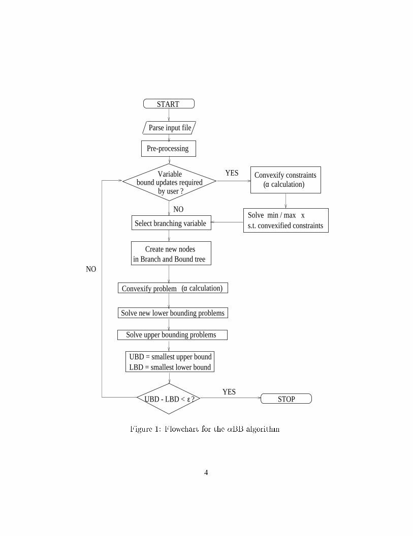
such as branching schemes, variable bound update strategies, automatic dif-ferentiation, interval arithmetic and a user-friendly parser, are outlined. Anextensive computational study is then carried out. The test problems chosenvary in size and type. The �rst series of examples consists of small problemsoften encountered in the literature. These are followed by chemical engineer-ing problems representing reactor network design, heat exchanger design andseparation system design. Then, a number of generalized geometric program-ming problems are addressed. Finally, some large batch scheduling problemswith uncertain parameters are solved.2 Algorithmic IssuesUsing the theoretical advances described in Part I of this paper (Adjimanet al., 1997), a user-friendly implementation of the algorithm was developed.The main objectives were to create an e�cient optimization environment forNLP problems involving twice-di�erentiable functions, while ensuring thatthe user interface remains simple and exible. The structure of the algorithm,illustrated in Figure 1, requires the implementation to possess the followingfeatures:� several alternatives for the construction of the lower bounding problem,depending on the mathematical characteristics of the terms appearingin the problem,� an interface with MINOPT (Schweiger et al., 1997), which contains acollection of local NLP and MINLP solvers.� the capability to derive Hessian matrices (second-order derivatives) orcharacteristic polynomials via automatic di�erentiation,� the ability to generate interval Hessian matrices and to perform intervalarithmetic,� � calculation functions for each of the methods presented in Part I,� several branching strategies,� several variable bounds update strategies.3

Solve min / max x

α calculation)(

UBD = smallest upper boundLBD = smallest lower bound

START

Variable bound updates required

by user ?

Select branching variable

εUBD - LBD < ? STOP

α calculation)(Convexify problem

s.t. convexified constraints

Solve upper bounding problems

Parse input file

Pre-processing

Convexify constraintsYES

NO

YES

NOin Branch and Bound tree

Create new nodes

Solve new lower bounding problems

Figure 1: Flowchart for the �BB algorithm4

The following discussion outlines the branching and variable boundingrules which are used in order to enhance the performance of the �BB algo-rithm. It also gives the rationale for the design of the di�erent componentsof the current implementation of the �BB algorithm.2.1 Branching StrategiesAlthough it does not present any theoretical di�culties, the branching stepof any branch-and-bound algorithm often has a signi�cant e�ect on the rateof convergence. This is especially true of the �BB algorithm as the quality ofthe underestimator depends on the variable bounds in a variety of ways. Forinstance, if a variable participates only linearly in the problem, branchingon it will not have any e�ect on the accuracy of the convex lower boundingfunctions. On the other hand, reducing the range of a variable raised toa high power is likely to result in much tighter underestimating problems.To take advantage of these observations, the implementation of the �BBalgorithm o�ers some choice in the selection of branching strategies. Fouralternatives are currently available:1. Use k-section on all or some of the variables.2. Use a measure of the quality of each term's underestimator, based onthe maximum separation distance between term and underestimator.3. Use a measure of the quality of each term's underestimator, based onthe separation distance at the optimum point.4. Use a measure of the overall in uence of each variable on the qualityof the lower bounding problem.2.1.1 Strategy 1By default, bisection on all the variables is used. The user can howeverspecify a restricted list of variables on which to branch. The interval to bebisected is determined through the `least reduced axis' rule whose applicationinvolves the calculation of a `current range to original range ratio', ri, foreach variable: ri = xUi � xLixUi;0 � xLi;0 (3)5

where xUi;0 and xLi;0 are respectively the upper and lower bound on variable xiat the �rst node of the branch-and-bound tree, and xUi and xLi are respectivelythe upper and lower bound on variable xi at the current node of the tree.The variable with the largest ri is selected for branching.2.1.2 Strategy 2While the second branching option requires additional computational e�ort,it results in a signi�cant improvement of the convergence time for di�cultproblems. A di�erent measure � is de�ned for each type of underestimator tofacilitate the assessment of the quality of the lower bounding function. Themaximum separation distance between the underestimator and the actualterm at the optimal solution of the lower bound problem is one possibleindicator of the degree of accuracy achieved in the construction of the convexapproximation. For a bilinear term xy, the maximum separation distance wasderived by Androulakis et al. (1995) so that �b is�b = (xU � xL)(yU � yL)4 : (4)For a fractional term, the maximum separation distance is derived in Ad-jiman et al. (1998). For trilinear and fractional trilinear terms, an exactformula for the maximum separation distance cannot be derived. The sep-aration distance at the optimum solution or an estimate of the maximumdistance must therefore be used (Adjiman et al., 1998).For a univariate concave term ut(x), the maximum separation distancecan be expressed as an optimization problem so that �u is given by�u = � minxL�x�xU �ut(x) + utL(x) (5)where utL(x) is the linearization of ut(x) around xL. Since ut(x) is con-cave and utL(x) is linear, the above optimization problem is convex and cantherefore be solved to global optimality.For a general nonconvex term, the maximum separation distance was derivedby Maranas and Floudas (1994) and the term measure is�� = 14Xi �i(xUi � xLi )2 (6)where the �i's are de�ned by Equation (2).6

Given a node to be partitioned, the values of �b, �u and �� are calculatedfor each term in accordance with its type. The term which appears to havethe worst underestimator or, in other words, the largest �, is then used as abasis for the selection of the branching variable. Out of the set of variablesthat participate in that term, the one with the `least reduced axis', as de�nedby Equation (3), is chosen for k-section. With this strategy, the in uence ofvariable bounds on the quality of the underestimators is taken into account,and hence this adaptive branching scheme ensures the e�ective tightening ofthe lower bounding problem from iteration to iteration.2.1.3 Strategy 3This strategy is a variant of Strategy 2. Instead of computing the maximumseparation distance between a term and its underestimator, their separationdistance at the optimum solution of the lower bounding problem is used.Thus, the bilinear term measure is now�b = jx�y� � w�j (7)where w is the variable which has been substituted for the bilinear term xyin order to construct its convex envelope (Adjiman et al., 1997) and the �superscript denotes the value of the variable at the solution of the currentlower bounding problem. The measures �t, �f and �ft, for trilinear, fractionaland fractional trilinear terms, are obtained in a similar fashion.The measure for univariate term ut(x) is�u = ut(x�)� utL(x�): (8)Finally, the general nonconvex term measure is�� = nXi=1 �i(xUi � x�i )(x�i � xLi ): (9)2.1.4 Strategy 4The fourth branching procedure takes the approach of Strategy 3 one stepfurther by considering the overall in uence of each variable on the convexproblem. After the relevant measures �b, �t, �f , �ft, �u and �� have been7

calculated for every term, a measure �v of each variable's contribution maybe obtained as follows:�iv = Xj2Bi �jb + Xj2Ti �jt + Xj2Fi �jf + Xj2FTi �jft + Xj2Ui �ju + Xj2Ni �j� (10)where �iv is the measure for the ith variable; Bi is the index set of thebilinear terms in which the ith variable participates, �jb is the measure of thejth bilinear term; Ti is the index set of the trilinear terms in which the ithvariable participates, �jt is the measure of the jth trilinear term; Fi is theindex set of the fractional terms in which the ith variable participates, �jf isthe measure of the jth fractional term; FTi is the index set of the fractionaltrilinear terms in which the ith variable participates, �jft is the measure ofthe jth fractional trilinear term; Ui is the index set of the univariate concaveterms in which the ith variable participates, �ju is the measure of the jthunivariate concave term; Ni is the index set of the general nonconvex termsin which the ith variable participates, �j� is the measure of the jth generalnonconvex term.The variable with the largest measure �v is selected as the branchingvariable, and k-section can be performed on it. If two or more variables havethe same �v, the `least reduced axis' test is performed to distinguish them.As will become apparent in the computational studies, branching strate-gies 2, 3 and 4 are particularly e�ective since they take into account thesensitivity of the underestimators to the bounds used for each variable.2.2 Variable Bound UpdatesThe quality of the convex lower bounding problem can also be improved byensuring that the variable bounds are as tight as possible. In the currentimplementation of the �BB algorithm, variable bound updates can either beperformed at the onset of an �BB run or at each iteration.In both cases, the same procedure is followed in order to construct thebound update problem. Given a solution domain, the convex underestimatorfor every constraint in the original problem is formulated. The bound problemfor variable xi is then expressed asxL;NEWi =xU;NEWi = 8>><>>: minx =maxx xis:t: G(x) � 0xL � x � xU (11)8

where G(x) are the convex underestimators of the constraints, and the boundson the variables, xL and xU are the best calculated bounds. Thus, once a newlower bound xL;NEWi on xi has been computed via a minimization, this valueis used in the formulation of the maximization problem for the generation ofan upper bound xU;NEWi .Because of the computational expense incurred by an update of thebounds on all variables, it is often desirable to de�ne a smaller subset of thevariables on which this operation is to be performed. The criterion devisedfor the selection of the branching variables can be used in this instance, sinceit provides a measure of the sensitivity of the problem to each variable. Anoption was therefore set up, in which bound updates are carried out only fora fraction of the variables with a non-zero �v, as calculated in Equation (10).2.3 Implementation IssuesThe goal of the implementation of the �BB algorithm is to produce a user-friendly global optimization environment which is reliable and exible. Thissection describes the choices made in order to meet these objectives.All the strategies for branching variable selection and variable boundupdates presented here, as well as the underestimation techniques proposedin Part I of this paper (Adjiman et al., 1997) have been implemented as partof the �BB package. In addition, an intuitive interface and a user's manual(Adjiman et al., 1997) have been designed.2.3.1 Problem Input and Pre-ProcessingTo a large extent, the practical value of a general optimization package ismeasured by its ability to solve a variety of problems. However, it must alsobe easily adapted to di�erent problem types so that no substantial transfor-mations are required from the user. The need for the second-order deriva-tives of the nonconvex functions in the problem raises practical di�cultiesin terms of the implementation of the algorithm and the format of the input�le. Because the problems solved belong to a very broad class for whichno structural assumptions may be made a priori, these derivatives must ei-ther be supplied by the user or generated automatically. The �rst optionwould be very cumbersome and would render the use of the �BB algorithmfastidious. In order to generate the derivatives automatically, the functionsmust be available in a code list format (Rall, 1981) which allows systematic9

di�erentiation based on elementary rules. Although the functions could beprovided by the user in this codi�ed notation, such an approach would resultin counter-intuitive problem input. By designing an interface which acceptsinput in standard mathematical notation, transforms it into the desired formand automatically generates sparse Jacobian and Hessian matrices, both easeof use and exibility can be achieved. The front-end parser developed as partof the �BB implementation creates this code list, while giving much freedomof notation to the user. This parser can also be used to input user-providedexpressions for the second order derivatives when these cannot be obtainedautomatically. During the parsing phase of an �BB run, the following tasksare carried out:� Identify variable, function, and parameter names.� De�ne linear, bilinear, trilinear, fractional, fractional trilinear, con-vex, univariate concave, and general nonconvex terms. This determineswhat types of underestimators are to be used.� Build code lists for the functions.� De�ne bounds on the solution space.� Gather optional information such as branching strategy, user-de�ned �values if any, etc.The choice of all names (variable, function, term, parameter) is left up tothe user, with the possibility to use index notation. Many index operationsare supported, such as summation, multiplication, enumeration and indexarithmetic. The input can therefore be made as explicit or as compact asdesired. A sample input �le for the CSTR sequence design problem discussedin Section 3.3.1 is listed in Appendix A. The formulation of this problem isgiven in Appendix B.Once the parsing phase is completed, a processing stage is initiated inwhich the code list for each of the lower bounding functions is built using theterm information provided in the input �le. Sparse Jacobians and Hessianmatrices are also generated in the code list format. The sparsity issue iscritical not only from the point of view of memory requirements, but alsowith respect to the diagonal shift matrix computation: the speed of thisprocess is strongly dependent on the number of participating variables for allthe methods described in Part I of this paper (Adjiman et al., 1997).10

Once all the necessary information has been gathered, the main iterationloop can be started.2.3.2 User-Speci�ed UnderestimatorsIn some instances, the problem to be solved may involve functions for whichno explicit formulation is available. The potential energy function for pro-teins, for example, is typically calculated using force-�eld models such asCHARMM (Brooks et al., 1983), AMBER (Weiner et al., 1986) or theECEPP/3 model (N�emethy et al., 1992). The user can require that these beused for function evaluations, as long as the Jacobian and a convex underes-timator are also provided.Some functions whose analytical form is entered in the input �le mayexhibit a special structure for which a tight underestimator is known. Thistailored lower bounding function can then be entered in the input �le andreplace the generic nonconvex underestimator of Equation (2).Similarly, if values or formulae have been derived for the � parameters,this information can be used by the algorithm, thereby improving its perfor-mance.2.3.3 � CalculationsTwo main options are available to the user for the determination of the �values to be used in the lower bounding problem.Option 1: User-speci�ed expressions supplied in the input �le for � com-putations.Option 2: Calculation using one of the automatic computation methodsdescribed in Part I (Adjiman et al., 1997).The successful implementation of the second option requires the avail-ability of a rigorous procedure for interval function evaluations. The �BBalgorithm is therefore connected to a C++ interval arithmetic library, PRO-FIL/BIAS, developed by Kn�uppel (1993). All the interval calculations arecarried out using the natural extension form of the functions (Ratschek andRokne, 1988). The main feature of this form is its simplicity but more accu-rate results can be obtained using the centered form or the remainder form(Cornelius and Lohner, 1984), at increased computational expense. The11

nested form is particularly suited for the special case of polynomial functionsbecause of the quality of its results and the ease of computation.Most of the O(n3) methods for the computation of a uniform diagonalshift matrix require the calculation of the minimum and/or maximum eigen-value of real symmetric matrices. These matrices are usually dense and ofsmall size since only the variables that participate in the nonconvex termto be underestimated are taken into consideration when building the Hes-sian matrix. Some Netlib routines for the transformation of real symmet-ric matrices into symmetric tridiagonal matrices using orthogonal similaritytransformations and the rational QR method with Newton corrections weretranslated into C for this purpose. The code was also customized based onthe speci�c requirements of the �BB algorithm. For Method I.5, based onthe Kharitonov theorem (Kharitonov, 1979), a symbolic expansion of the de-terminant must be carried out and Leverrier's method (Wayland, 1945) wastherefore implemented. Although it is more computationally expensive thanKrylov's method or Danielewsky's method (Wayland, 1945), it is the onlyapproach which does not involve divisions by the Hessian elements. Thiseliminates the risk of encountering singularities when interval arithmetic issubsequently used.Finally, the error in the � parameter calculations is closely monitored toguarantee the global optimality of the �nal solution.3 Computational Case StudiesThe purpose of this section is to demonstrate the performance of the �BB al-gorithm in identifying the global minimum of nonconvex optimization prob-lems and to study the e�ects of the di�erent underestimating methods ofPart I (Adjiman et al., 1997) and the various convergence-enhancing schemespresented in the previous sections. First, some literature problems are tack-led, giving insights into the suggested branching and variable range reductionstrategies. Larger examples are then employed to test the algorithm. Allcomputational results were obtained on a HP9000/730 with a convergencetolerance of 0.001, unless speci�ed otherwise.12

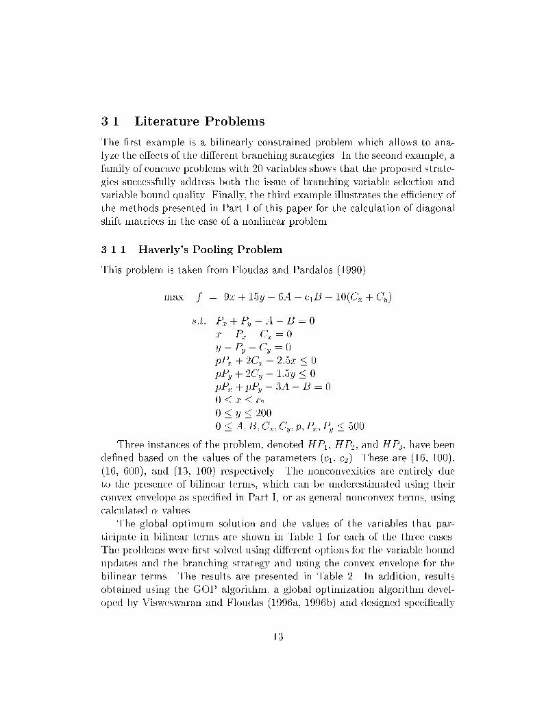
3.1 Literature ProblemsThe �rst example is a bilinearly constrained problem which allows to ana-lyze the e�ects of the di�erent branching strategies. In the second example, afamily of concave problems with 20 variables shows that the proposed strate-gies successfully address both the issue of branching variable selection andvariable bound quality. Finally, the third example illustrates the e�ciency ofthe methods presented in Part I of this paper for the calculation of diagonalshift matrices in the case of a nonlinear problem.3.1.1 Haverly's Pooling ProblemThis problem is taken from Floudas and Pardalos (1990).max f = 9x + 15y � 6A� c1B � 10(Cx + Cy)s:t: Px + Py � A� B = 0x� Px � Cx = 0y � Py � Cy = 0pPx + 2Cx � 2:5x � 0pPy + 2Cy � 1:5y � 0pPx + pPy � 3A�B = 00 � x � c20 � y � 2000 � A;B;Cx; Cy; p; Px; Py � 500Three instances of the problem, denoted HP1, HP2, and HP3, have beende�ned based on the values of the parameters (c1, c2). These are (16, 100),(16, 600), and (13, 100) respectively. The nonconvexities are entirely dueto the presence of bilinear terms, which can be underestimated using theirconvex envelope as speci�ed in Part I, or as general nonconvex terms, usingcalculated � values.The global optimum solution and the values of the variables that par-ticipate in bilinear terms are shown in Table 1 for each of the three cases.The problems were �rst solved using di�erent options for the variable boundupdates and the branching strategy and using the convex envelope for thebilinear terms. The results are presented in Table 2. In addition, resultsobtained using the GOP algorithm, a global optimization algorithm devel-oped by Visweswaran and Floudas (1996a, 1996b) and designed speci�cally13

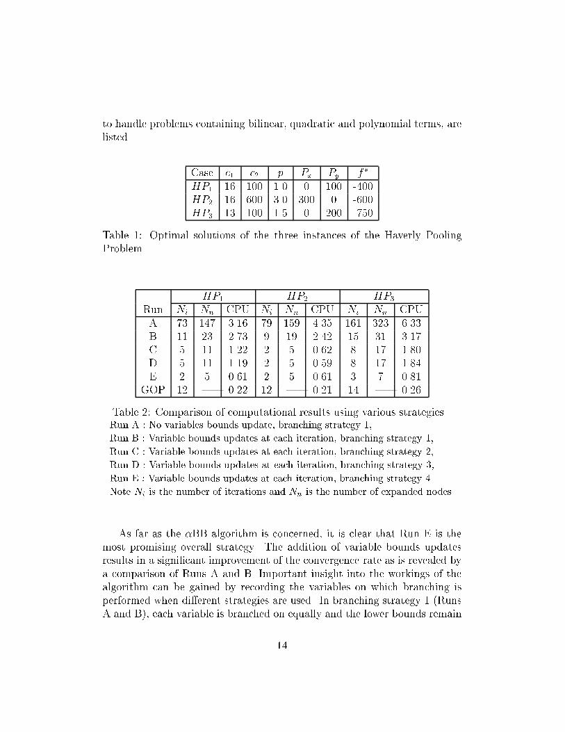
to handle problems containing bilinear, quadratic and polynomial terms, arelisted. Case c1 c2 p Px Py f �HP1 16 100 1.0 0 100 -400HP2 16 600 3.0 300 0 -600HP3 13 100 1.5 0 200 -750Table 1: Optimal solutions of the three instances of the Haverly PoolingProblem. HP1 HP2 HP3Run Ni Nn CPU Ni Nn CPU Ni Nn CPUA 73 147 3.16 79 159 4.35 161 323 6.33B 11 23 2.73 9 19 2.42 15 31 3.17C 5 11 1.22 2 5 0.62 8 17 1.80D 5 11 1.19 2 5 0.59 8 17 1.84E 2 5 0.61 2 5 0.61 3 7 0.81GOP 12 | 0.22 12 | 0.21 14 | 0.26Table 2: Comparison of computational results using various strategies.Run A : No variables bounds update, branching strategy 1,Run B : Variable bounds updates at each iteration, branching strategy 1,Run C : Variable bounds updates at each iteration, branching strategy 2,Run D : Variable bounds updates at each iteration, branching strategy 3,Run E : Variable bounds updates at each iteration, branching strategy 4.Note Ni is the number of iterations and Nn is the number of expanded nodes.As far as the �BB algorithm is concerned, it is clear that Run E is themost promising overall strategy. The addition of variable bounds updatesresults in a signi�cant improvement of the convergence rate as is revealed bya comparison of Runs A and B. Important insight into the workings of thealgorithm can be gained by recording the variables on which branching isperformed when di�erent strategies are used. In branching strategy 1 (RunsA and B), each variable is branched on equally and the lower bounds remain14

constant for several iterations as the variables participating linearly have lit-tle e�ect on the tightness of the underestimating problem. In other runs,branching depends on the term measure �b, either directly or through thevariable measure �v. Since the bilinear terms include three variables, p; Pxand Py, they are the only branching candidates. This leads to another con-siderable improvement in performance. With branching strategies 2 and 3,each one of the three variables is branched on equally. With branching strat-egy 4, however, p is branched on exclusively as it participates in all bilinearterms and its �v is always greater than that of Px or Py. The performance ofthe branch-and-bound search is therefore enhanced substantially by selectingappropriately the branching variables.Using the same branching and bounding options as in Run E, the prob-lems were then solved by treating the bilinear terms as general nonconvexterms. For bilinear terms, the Hessian matrix is independent of the variablesand no interval calculations are required. The minimum eigenvalue requiredby all uniform diagonal shift matrix methods is therefore easily obtained.Table 3 compares the performance of the algorithm using the convex enve-lope (\Linear") and �-based underestimation. The row labeled \Convex I"reports results obtained using a uniform diagonal shift matrix (a single �value per term), and \Convex II" was obtained using the scaled Gerschgorintheorem method which generates one � per variable in a nonconvex term.The use of � leads to looser lower bounding functions than the convex enve-lope. Moreover, it requires the solution of a convex NLP for the generationof a lower bound, whereas a linear program is constructed when the con-vex envelope is used. As a result, both computation time and number ofiterations increase signi�cantly. The exploitation of the special structure ofbilinear terms is thus expected to provide the best results in most cases. Forvery large problems, however, the introduction of additional variables andconstraints may become prohibitive and a convex underestimator becomesmore appropriate (Harding and Floudas, 1997).3.1.2 Linearly Constrained Concave Optimization ProblemsThis set of problems taken from Floudas and Pardalos (1990) will be usedto show the increased e�ciency of the algorithm when appropriate strategiesare being employed to select the variables whose bounds will be updated.The general form of the problems is as follows :15

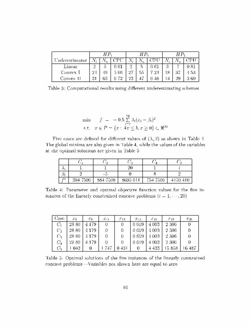
HP1 HP2 HP3Underestimator Ni Nn CPU Ni Nn CPU Ni Nn CPULinear 2 5 0.61 2 5 0.61 3 7 0.81Convex I 24 49 5.66 27 55 7.23 18 37 4.53Convex II 31 63 6.72 23 47 6.48 14 29 3.60Table 3: Computational results using di�erent underestimating schemes.min f = � 0:5 20Pi=1�i(xi � �i)2s:t: x 2 P = fx : Ax � b; x � 0g � <20Five cases are de�ned for di�erent values of (�; �) as shown in Table 4.The global minima are also given in Table 4, while the values of the variablesat the optimal solutions are given in Table 5.C1 C2 C3 C4 C5�i 1 1 20 1 i�i 2 -5 0 8 2f � -394.7506 -884.7508 -8695.011 -754.7506 -4150.410Table 4: Parameter and optimal objective function values for the �ve in-stances of the linearly constrained concave problems (i = 1; � � � ; 20).Case x3 x6 x11 x13 x15 x16 x18 x20C1 28.80 4.179 0 0 0.619 4.093 2.306 0C2 28.80 4.179 0 0 0.619 4.093 2.306 0C3 28.80 4.179 0 0 0.619 4.093 2.306 0C4 28.80 4.179 0 0 0.619 4.093 2.306 0C5 1.043 0 1.747 0.431 0 4.433 15.858 16.487Table 5: Optimal solutions of the �ve instances of the linearly constrainedconcave problems { Variables not shown here are equal to zero.16

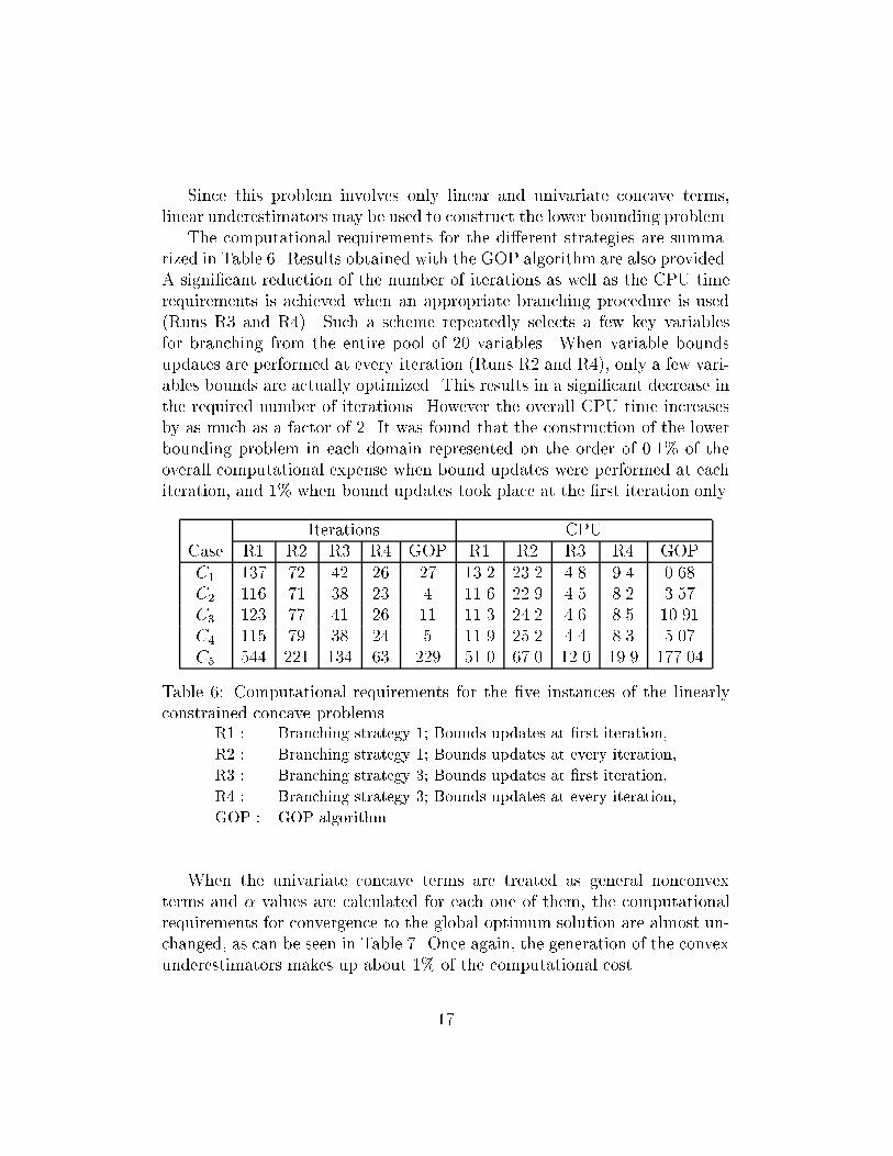
Since this problem involves only linear and univariate concave terms,linear underestimators may be used to construct the lower bounding problem.The computational requirements for the di�erent strategies are summa-rized in Table 6. Results obtained with the GOP algorithm are also provided.A signi�cant reduction of the number of iterations as well as the CPU timerequirements is achieved when an appropriate branching procedure is used(Runs R3 and R4). Such a scheme repeatedly selects a few key variablesfor branching from the entire pool of 20 variables. When variable boundsupdates are performed at every iteration (Runs R2 and R4), only a few vari-ables bounds are actually optimized. This results in a signi�cant decrease inthe required number of iterations. However the overall CPU time increasesby as much as a factor of 2. It was found that the construction of the lowerbounding problem in each domain represented on the order of 0.1% of theoverall computational expense when bound updates were performed at eachiteration, and 1% when bound updates took place at the �rst iteration only.Iterations CPUCase R1 R2 R3 R4 GOP R1 R2 R3 R4 GOPC1 137 72 42 26 27 13.2 23.2 4.8 9.4 0.68C2 116 71 38 23 4 11.6 22.9 4.5 8.2 3.57C3 123 77 41 26 11 11.3 24.2 4.6 8.5 10.91C4 115 79 38 24 5 11.9 25.2 4.4 8.3 5.07C5 544 221 134 63 229 51.0 67.0 12.0 19.9 177.04Table 6: Computational requirements for the �ve instances of the linearlyconstrained concave problems.R1 : Branching strategy 1; Bounds updates at �rst iteration,R2 : Branching strategy 1; Bounds updates at every iteration,R3 : Branching strategy 3; Bounds updates at �rst iteration,R4 : Branching strategy 3; Bounds updates at every iteration,GOP : GOP algorithm.When the univariate concave terms are treated as general nonconvexterms and � values are calculated for each one of them, the computationalrequirements for convergence to the global optimum solution are almost un-changed, as can be seen in Table 7. Once again, the generation of the convexunderestimators makes up about 1% of the computational cost.17

C1 C2 C3 C4 C5Underes. Ni CPU Ni CPU Ni CPU Ni CPU Ni CPULinear 42 4.8 38 4.5 41 4.6 38 4.4 134 12.0Convex 42 4.2 38 3.8 41 3.8 38 3.9 134 9.3Table 7: Computational results using di�erent underestimators for the lin-early constrained concave problems. Strategy R3 was used for all runs.3.1.3 Constrained Nonlinear Optimization ExampleThis is a small but nevertheless di�cult nonconvex problem from Murtaghand Saunders (1983). The �BB algorithm is very well suited for this examplesince it combines bilinear, univariate concave and general nonconvex terms.min (x1 � 1)2 + (x1 � x2)2 + (x2 � x3)3 + (x3 � x4)4 + (x4 � x5)4s.t. x1 + x22 + x33 = 3p2 + 2x2 � x23 + x4 = 2p2� 2x1x5 = 2xi 2 [�5; 5]; i = 1; � � � ; 5The global minimum as well as some local minima are presented in Ta-ble 8. obj x1 x2 x3 x4 x5Global 0.0293 1.1166 1.2204 1.5378 1.9728 1.7911Local 1 27.8719 -1.2731 2.4104 1.1949 -0.1542 -1.5710Local 2 44.0221 -0.7034 2.6357 -0.0963 -1.7980 -2.8434Local 3 52.9026 0.7280 -2.2452 0.7795 3.6813 2.7472Local 4 64.8740 4.5695 -1.2522 0.4718 2.3032 4.3770Table 8: Global and local minima of example 3.1.3.All the � calculation methods proposed in Part I of this paper have beenused to solve this problem to global optimality. Strategies 2, 3 or 4 wereused for branching variable selection and bound updates were performed18

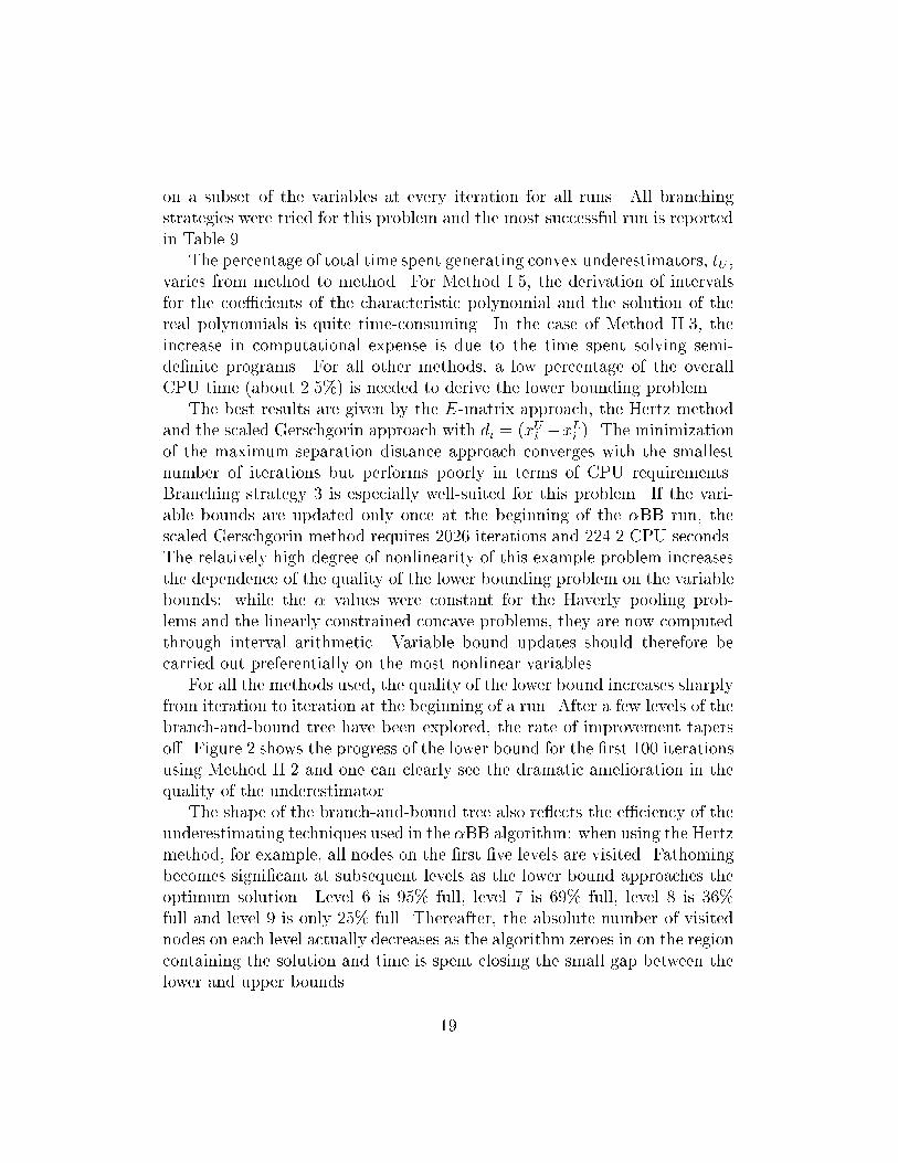
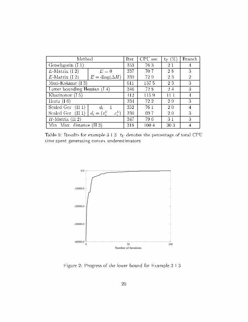
on a subset of the variables at every iteration for all runs. All branchingstrategies were tried for this problem and the most successful run is reportedin Table 9.The percentage of total time spent generating convex underestimators, tU ,varies from method to method. For Method I.5, the derivation of intervalsfor the coe�cients of the characteristic polynomial and the solution of thereal polynomials is quite time-consuming. In the case of Method II.3, theincrease in computational expense is due to the time spent solving semi-de�nite programs. For all other methods, a low percentage of the overallCPU time (about 2.5%) is needed to derive the lower bounding problem.The best results are given by the E-matrix approach, the Hertz methodand the scaled Gerschgorin approach with di = (xUi �xLi ). The minimizationof the maximum separation distance approach converges with the smallestnumber of iterations but performs poorly in terms of CPU requirements.Branching strategy 3 is especially well-suited for this problem. If the vari-able bounds are updated only once at the beginning of the �BB run, thescaled Gerschgorin method requires 2026 iterations and 224.2 CPU seconds.The relatively high degree of nonlinearity of this example problem increasesthe dependence of the quality of the lower bounding problem on the variablebounds: while the � values were constant for the Haverly pooling prob-lems and the linearly constrained concave problems, they are now computedthrough interval arithmetic. Variable bound updates should therefore becarried out preferentially on the most nonlinear variables.For all the methods used, the quality of the lower bound increases sharplyfrom iteration to iteration at the beginning of a run. After a few levels of thebranch-and-bound tree have been explored, the rate of improvement taperso�. Figure 2 shows the progress of the lower bound for the �rst 100 iterationsusing Method II.2 and one can clearly see the dramatic amelioration in thequality of the underestimator.The shape of the branch-and-bound tree also re ects the e�ciency of theunderestimating techniques used in the �BB algorithm: when using the Hertzmethod, for example, all nodes on the �rst �ve levels are visited. Fathomingbecomes signi�cant at subsequent levels as the lower bound approaches theoptimum solution. Level 6 is 95% full, level 7 is 69% full, level 8 is 36%full and level 9 is only 25% full. Thereafter, the absolute number of visitednodes on each level actually decreases as the algorithm zeroes in on the regioncontaining the solution and time is spent closing the small gap between thelower and upper bounds. 19

Method Iter. CPU sec. tU (%) BranchGerschgorin (I.1) 353 76.3 2.1 4E-Matrix (I.2) E = 0 337 70.7 2.8 3E-Matrix (I.2) E = diag(�H) 339 72.9 2.3 2Mori-Kokame (I.3) 611 137.5 2.3 3Lower bounding Hessian (I.4) 346 72.8 2.4 3Kharitonov (I.5) 412 115.9 11.1 4Hertz (I.6) 334 72.2 2.9 3Scaled Ger. (II.1) di = 1 352 76.1 2.0 4Scaled Ger. (II.1) di = (xUi � xLi ) 330 69.7 2.0 3H-Matrix (II.2) 347 79.6 3.1 3Min. Max. distance (II.3) 318 100.4 30.3 4Table 9: Results for example 3.1.3. tU denotes the percentage of total CPUtime spent generating convex underestimators.

0 50 100Number of Iterations

-40000.0

-30000.0

-20000.0

-10000.0

0.0

Figure 2: Progress of the lower bound for Example 3.1.3.20

3.2 Chemical Engineering Design ProblemsHaving established the importance of branching variable selection and vari-able bound updates, some results will now be presented for a set of optimiza-tion formulations for chemical process design problems. The �rst problemis a small reactor network design problem, the second example is a heat ex-changer network design problem and the third is a separation network designproblem.3.2.1 Reactor Network DesignThe following example, taken from Ryoo and Sahinidis (1995), is a reactornetwork design problem, describing the system shown in Figure 3.A B C A B C

K4

x1 = Ca,1x3 = Cb, 1

x2 = Ca,2x4 = Cb,2x5 = V1 x6 = V2

K1 K3 K2

Figure 3: Reactor Network Design Problem.This problem is known to have caused di�culties for other global opti-mization methods. min�x4s.t. x1 + k1x1x5 = 1x2 � x1 + k2x2x6 = 0x3 + x1 + k3x3x5 = 121

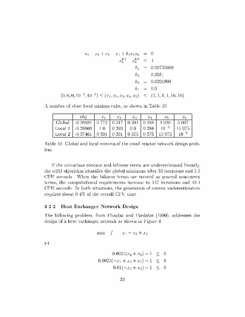
x4 � x3 + x2 � x1 + k4x4x6 = 0x0:55 + x0:56 � 4k1 = 0:09755988k2 = 0:99k1k3 = 0:0391908k4 = 0:9(0; 0; 0; 10�5; 10�5) � (x1; x2; x3; x4; x5) � (1; 1; 1; 1; 16; 16)A number of close local minima exist, as shown in Table 10.obj x1 x2 x3 x4 x5 x6Global -0.38881 0.772 0.517 0.204 0.388 3.036 5.097Local 1 -0.38808 1.0 0.393 0.0 0.388 10�5 15.975Local 2 -0.37461 0.391 0.391 0.375 0.375 15.975 10�5Table 10: Global and local minima of the small reactor network design prob-lem.If the univariate concave and bilinear terms are underestimated linearly,the �BB algorithm identi�es the global minimum after 33 iterations and 5.5CPU seconds. When the bilinear terms are treated as general nonconvexterms, the computational requirements increase to 157 iterations and 43.4CPU seconds. In both situations, the generation of convex underestimatorsrequires about 0.4% of the overall CPU time.3.2.2 Heat Exchanger Network DesignThe following problem, from Floudas and Pardalos (1990), addresses thedesign of a heat exchanger network as shown in Figure 4.min f = x1 + x2 + x3s.t. 0:0025(x4 + x6)� 1 � 00:0025(�x4 + x5 + x7)� 1 � 00:01(�x5 + x8)� 1 � 022

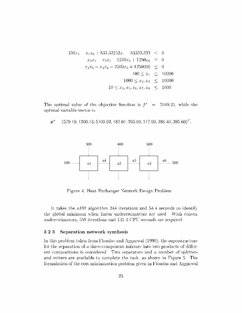
100x1 � x1x6 + 833:33252x4 � 83333:333 � 0x2x4 � x2x7 � 1250x4 + 1250x5 � 0x3x5 � x3x8 � 2500x5 + 1250000 � 0100 � x1 � 100001000 � x2; x3 � 1000010 � x4; x5; x6; x7; x8 � 1000The optimal value of the objective function is f � = 7049:25, while theoptimal variable vector isx� = (579:19; 1360:13; 5109:92; 182:01; 295:60; 217:99; 286:40; 395:60)T:100 x1 x2 x3

x5x4 x6

300 400 600

500

Figure 4: Heat Exchanger Network Design Problem.It takes the �BB algorithm 244 iterations and 54.4 seconds to identifythe global minimum when linear underestimators are used. With convexunderestimators, 558 iterations and 141.4 CPU seconds are required.3.2.3 Separation network synthesisIn this problem taken from Floudas and Aggarwal (1990), the superstructurefor the separation of a three-component mixture into two products of di�er-ent compositions is considered. Two separators and a number of splittersand mixers are available to complete the task, as shown in Figure 5. Theformulation of the cost minimization problem given in Floudas and Aggarwal23

(1990) has been slightly modi�ed to reduce the number of variables. It nowinvolves 22 variables and 16 equality constraints. It is expressed asmin 0:9979 + 0:00432F1 + 0:00432F13 + 0:01517F2 + 0:01517F9s.t F1 + F2 + F3 + F4 = 300F5 � F6 � F7 = 0F8 � F9 � F10 � F11 = 0F12 � F13 � F14 � F15 = 0F16 � F17 � F18 = 0F13xA;12 � F5 + 0:333 � F1 = 0F13xB;12 � F8xB;8 + 0:333 � F1 = 0�F8xC;8 + 0:333F1 = 0�F12xA;12 � 0:333F2 = 0F9xB;8 � F12xB; 12 + 0:333F2 = 0F9xC;8 � F16 + 0:333F2 = 0F14xA;12 + 0:333F3 + F6 = 30F10xB;8 + F14xB;12 + 0:333F3 = 50F10xC;8 + 0:333F3 + F17 = 30xB;8 + xC;8 = 1xA;12 + xB;12 = 10 � Fi � 1500 � xi;j � 1where Fi denotes the total owrate of the ith stream and xj;i denotes thefraction of component j in the ith stream.The global optimal con�guration is identi�ed in Figure 6. The optimalconcentrations are xB;8 = xC;8 = 0:5, xA;12 = 0 and xB;12 = 1. The optimalnon-zero owrates are F1 = 60, F3 = 90, F4 = 150, F5 = F7 = 20, F8 = F9 =40, F12 = F14 = 20 and F16 = F18 = 20.24

BC

F1

F2 P2

F15

F3 F4

II

F16

F18

F12 F15

F8

F9

F5

A

17

P1I

F6

F7F10

F11

F14

FFigure 5: Superstructure for example 3.2.3.BC

P2II

F1

A

P1

4

I

F

F

F

9

8

5

F7

F12

F14

F3

F16F18

FFigure 6: Optimal con�guration for example 3.2.3.The algorithm converged to the global solution in 15.2 CPU seconds andafter 11 iterations, when the bilinear terms were underestimated linearly.When they were treated as general nonconvex terms, 49 iterations and 220.1CPU seconds were required. 25

3.3 Generalized Geometric Programming ProblemsMany important design and control problems can be formulated as general-ized geometric programming problems, a subclass of the twice-di�erentiableproblems that the �BB algorithm can address. The main property of thefunctions involved in the formulation is that they are the algebraic sum ofposynomials, terms of the form c nQi=1 xdii where c is a positive real number,the xi's are positive real variable and the di's are scalars. No restrictions ofintegrality or positivity are imposed on the exponents. Maranas and Floudas(1997) proposed a new approach to tackle such problems, based on a di�er-ence of convex functions transformation embedded in a branch-and-boundframework. In this section, we show that the �BB can be successfully usedon this class of problems and we report results for the example problemstreated in Maranas and Floudas (1997).Two design problems were studied in the area of chemical process engi-neering: an alkylation design problem and the design of a CSTR sequencesubject to some capital cost constraints. The objective was to minimizecost or to maximize production. The aim of the six control problems wasto carry out the stability analysis of some nonlinear systems with uncertainparameters. These examples were therefore formulated as the minimizationof the stability margin, k, and the system was deemed unstable if the opti-mal solution was found to be less than unity. Two approaches can be usedto treat such problems, the �rst relying on the identi�cation of the smallestpossible value of k, and the second testing the feasibility of the problem withk 2 [0; 1]. The alkylation problem was discussed in detail in Part I of thispaper. All other problem formulations are given in Appendix B.3.3.1 CSTR Sequence DesignFollowing the reformulation proposed in Maranas and Floudas (1997) forexample 3.2.1, the objective function is expressed as a ratio of polynomialsand is subject to a single nonlinear constraint. The reactor volumes are theonly two variables. The problem is solved for two sets of reaction constants.Since there is only one constraint, which relates the two reactor vol-umes, variable bound updates are very fast. Yet, as is apparent in Table 11,the reduction in overall iteration number achieved when bound updates areperformed at each iteration results in an increase in the computational re-quirements. This example and the alkylation problem (Adjiman et al., 1997)26

seem to indicate that problems belonging to the class of generalized geomet-ric programming can be treated using a single bound update before the �rstiteration.For this problem the use of a single � per term or of one � per variabledoes not have much in uence on the performance of the algorithm. Uponexamining the functions in the problem, it appears that the variables partic-ipate in very similar ways, therefore contributing to the nonconvexity to thesame degree.Finally, the performance of the algorithm for this highly nonlinear formu-lation is better, in terms of CPU time, than for the simpler formulation ofexample 3.2.1 which involves only bilinear terms. It therefore seems worth-while to reduce the number of variables, even at the expense of functionalsimplicity.3.3.2 Stability Analysis of Nonlinear SystemsExample 1 This problem involves 4 variables and 4 constraints, one ofwhich is nonlinear. The system is found to be unstable with k = 0:3417. Theresults shown in Table 12 were obtained with the third branching strategy,using a single bound update. They correspond to the solution of the globaloptimality problem, in which wide bounds on k are used to try and identifythe smallest possible value. If the actual value of the stability margin is ofno interest, the feasibility problem can be solved, in which the value of k isrestricted to [0; 1]. In such a case, the algorithm can terminate when an upperbound on k has been found within this interval (the system is unstable), orwhen infeasibility has been asserted (the system is stable). For this example,a satisfactory upper bound, proving stability, is obtained in less than 1 CPUsec.Example 2 Contrary to the previous example, this 4 variable system isstable, with a stability margin of k = 1:089. In order to prove that thesystem is stable, one must show that the feasibility problem has no solution.Alternatively, the minimum stability margin can be identi�ed using widerbounds on k. Clearly, global optimality runs are more time demanding asthey span a larger solution space. The results are shown in Table 13.Example 3 The global optimum solution of k = 0:8175 is identi�ed usingthe fourth branching strategy and a single bound update. The fact that the27

First set of reaction rate constantsSingle Update One Update/IterMethod Iter. CPU tU Iter. CPU tUsec. (%) sec. (%)Gerschgorin (I.1) 101 4.5 28.9 67 7.1 15.8E-Matrix (I.2) E = 0 94 4.4 28.6 67 7.0 16.3E-Matrix (I.2) E = diag(�H) 105 4.6 30.2 68 7.2 17.0Mori-Kokame (I.3) 137 6.1 39.1 89 8.9 17.9Lower bounding Hessian (I.4) 94 4.3 31.6 67 6.7 16.5Kharitonov (I.5) 123 21.3 66.6 81 24.4 51.7Hertz (I.6) 94 4.4 41.4 67 6.8 21.2Scaled G. (II.1) di = 1 101 4.5 27.8 66 6.6 20.2Scaled G. (II.1) di = (xUi � xLi ) 92 4.2 21.9 63 6.5 15.3H-Matrix (II.2) 94 4.2 16.9 65 6.7 17.7Min. Max. distance (II.3) 93 6.3 40.1 62 8.0 29.1Second set of reaction rate constantsSingle Update One Update/IterMethod Iter. CPU tU Iter. CPU tUsec. (%) sec. (%)Gerschgorin (I.1) 111 4.9 24.1 75 7.7 18.1E-Matrix (I.2) E = 0 109 4.7 29.0 67 7.0 18.2E-Matrix (I.2) E = diag(�H) 114 5.1 24.1 79 8.0 21.1Mori-Kokame (I.3) 150 6.4 25.9 95 9.8 17.8Lower bounding Hessian (I.4) 109 4.7 26.8 74 7.5 15.2Kharitonov (I.5) 135 15.6 61.5 84 16.8 46.7Hertz (I.6) 109 4.7 23.0 74 7.5 17.9Scaled G. (II.1) di = 1 109 4.6 26.2 74 7.5 18.9Scaled G. (II.1) di = (xUi � xLi ) 105 4.6 24.2 72 7.3 17.8H-Matrix (II.2) 109 4.6 17.7 74 7.6 15.1Min. Max. distance (II.3) 107 6.8 43.4 73 9.2 30.0Table 11: Results for Example 3.3.1. tU denotes the percentage of total CPUtime spent generating convex underestimators.28

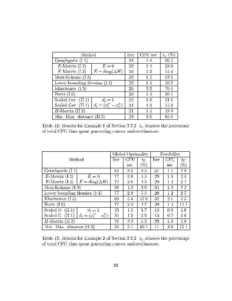
Method Iter. CPU sec. tU (%)Gerschgorin (I.1) 24 1.4 26.5E-Matrix (I.2) E = 0 20 1.4 28.9E-Matrix (I.2) E = diag(�H) 20 1.3 15.4Mori-Kokame (I.3) 20 1.2 23.1Lower bounding Hessian (I.4) 20 1.4 16.2Kharitonov (I.5) 20 3.3 70.5Hertz (I.6) 20 1.4 20.5Scaled Ger. (II.1) di = 1 22 1.6 11.1Scaled Ger. (II.1) di = (xUi � xLi ) 21 1.3 15.2H-Matrix (II.2) 21 1.4 19.3Min. Max. distance (II.3) 18 8.6 85.0Table 12: Results for Example 1 of Section 3.3.2. tU denotes the percentageof total CPU time spent generating convex underestimators.Global Optimality FeasibilityMethod Iter. CPU tU Iter. CPU tUsec. (%) sec. (%)Gerschgorin (I.1) 82 3.0 3.5 31 1.1 7.9E-Matrix (I.2) E = 0 77 2.8 5.5 29 1.8 2.5E-Matrix (I.2) E = diag(�H) 74 2.6 4.5 29 1.2 2.1Mori-Kokame (I.3) 98 1.3 3.6 34 1.3 7.3Lower bounding Hessian (I.4) 77 2.8 5.5 29 1.2 2.7Kharitonov (I.5) 89 5.4 57.6 32 2.1 5.5Hertz (I.6) 77 2.3 4.7 29 1.2 11.1Scaled G. (II.1) di = 1 43 1.5 1.7 13 0.8 5.6Scaled G. (II.1) di = (xUi � xLi ) 35 1.2 2.0 13 0.7 5.6H-Matrix (II.2) 76 3.3 5.2 29 1.6 2.8Min. Max. distance (II.3) 34 5.1 86.1 11 2.9 75.1Table 13: Results for Example 2 of Section 3.3.2. tU denotes the percentageof total CPU time spent generating convex underestimators.29

system is unstable is identi�ed in under 1 CPU sec. The results of the globaloptimality problem are shown in Table 14.Method Iter. CPU sec. tU (%)Gerschgorin (I.1) 20 1.0 4.3E-Matrix (I.2) E = 0 18 0.9 4.2E-Matrix (I.2) E = diag(�H) 17 0.9 3.7Mori-Kokame (I.3) 17 0.8 4.2Lower bounding Hessian (I.4) 20 1.0 4.0Kharitonov (I.5) 18 1.1 31.0Hertz (I.6) 18 0.8 4.2Scaled Ger. (II.1) di = 1 17 0.8 4.2Scaled Ger. (II.1) di = (xUi � xLi ) 12 0.6 5.3H-Matrix (II.2) 17 0.9 4.4Min. Max. distance (II.3) 26 2.1 37.6Table 14: Results for Example 3 of Section 3.3.2. tU denotes the percentageof total CPU time spent generating convex underestimators.Example 4 With a minimum stability margin of 6:27, this system is stable.The perturbation frequency !, which was eliminated from previous formu-lations, is kept in this example. At the global optimum solution, the valueof ! is 0.986. The bounds used for this variable have a signi�cant e�ect onthe convergence rate of the algorithm. To illustrate this point, the feasibilityproblem was solved with ! 2 [0; 1] and ! 2 [0; 10]. The fourth branchingstrategy was used and a single variable bound update was performed. Theresults are shown in Table 15.Example 5 This formulation is used to determine the stability of DaimlerBenz bus. It involves 4 variables and the exponent values range from 1 to 8.The minimum stability margin is k = 1:2069 and the problem is treated asa feasibility problem. The results are shown in Table 16.Example 6 This �nal problem was developed to study the stability ofthe Fiat Dedra spark ignition engine. It involves 9 variables and is highlynonlinear. The solution of the stability problem shows that this system is30

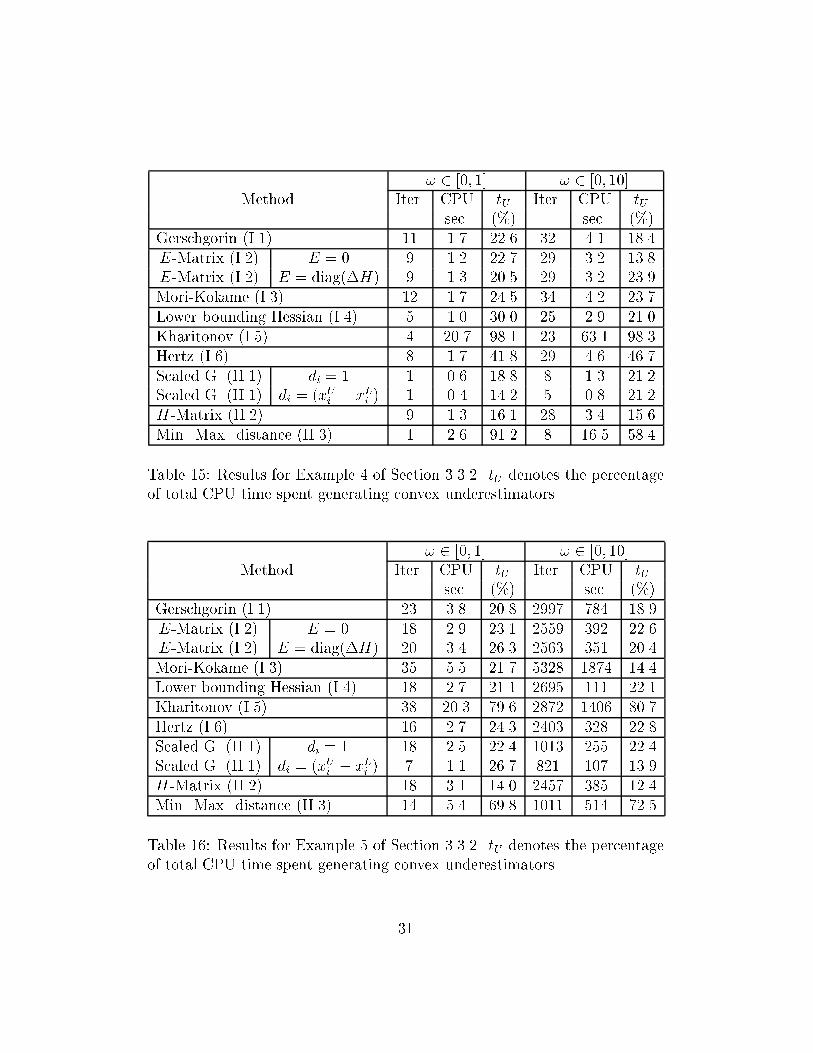
! 2 [0; 1] ! 2 [0; 10]Method Iter. CPU tU Iter. CPU tUsec. (%) sec. (%)Gerschgorin (I.1) 11 1.7 22.6 32 4.1 18.4E-Matrix (I.2) E = 0 9 1.2 22.7 29 3.2 13.8E-Matrix (I.2) E = diag(�H) 9 1.3 20.5 29 3.2 23.9Mori-Kokame (I.3) 12 1.7 24.5 34 4.2 23.7Lower bounding Hessian (I.4) 5 1.0 30.0 25 2.9 21.0Kharitonov (I.5) 4 20.7 98.1 23 63.1 98.3Hertz (I.6) 8 1.7 41.8 29 4.6 46.7Scaled G. (II.1) di = 1 1 0.6 18.8 8 1.3 21.2Scaled G. (II.1) di = (xUi � xLi ) 1 0.4 14.2 5 0.8 21.2H-Matrix (II.2) 9 1.3 16.1 28 3.4 15.6Min. Max. distance (II.3) 1 2.6 91.2 8 16.5 58.4Table 15: Results for Example 4 of Section 3.3.2. tU denotes the percentageof total CPU time spent generating convex underestimators.! 2 [0; 1] ! 2 [0; 10]Method Iter. CPU tU Iter. CPU tUsec. (%) sec. (%)Gerschgorin (I.1) 23 3.8 20.8 2997 784 18.9E-Matrix (I.2) E = 0 18 2.9 23.1 2559 392 22.6E-Matrix (I.2) E = diag(�H) 20 3.4 26.3 2563 351 20.4Mori-Kokame (I.3) 35 5.5 21.7 5328 1874 14.4Lower bounding Hessian (I.4) 18 2.7 21.1 2695 111 22.1Kharitonov (I.5) 38 20.3 79.6 2872 1406 80.7Hertz (I.6) 16 2.7 24.3 2403 328 22.8Scaled G. (II.1) di = 1 18 2.5 22.4 1013 255 22.4Scaled G. (II.1) di = (xUi � xLi ) 7 1.1 26.7 821 107 13.9H-Matrix (II.2) 18 3.1 14.0 2457 385 12.4Min. Max. distance (II.3) 14 5.4 69.8 1011 514 72.5Table 16: Results for Example 5 of Section 3.3.2. tU denotes the percentageof total CPU time spent generating convex underestimators.31

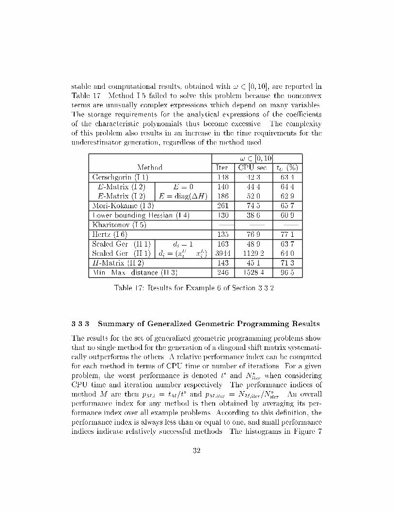
stable and computational results, obtained with ! 2 [0; 10], are reported inTable 17. Method I.5 failed to solve this problem because the nonconvexterms are unusually complex expressions which depend on many variables.The storage requirements for the analytical expressions of the coe�cientsof the characteristic polynomials thus become excessive. The complexityof this problem also results in an increase in the time requirements for theunderestimator generation, regardless of the method used.! 2 [0; 10]Method Iter. CPU sec. tU (%)Gerschgorin (I.1) 148 42.3 63.4E-Matrix (I.2) E = 0 140 44.4 64.4E-Matrix (I.2) E = diag(�H) 186 52.0 62.9Mori-Kokame (I.3) 261 74.5 65.7Lower bounding Hessian (I.4) 130 38.6 60.9Kharitonov (I.5) | | |Hertz (I.6) 135 76.9 77.1Scaled Ger. (II.1) di = 1 163 48.9 63.7Scaled Ger. (II.1) di = (xUi � xLi ) 3944 1129.2 64.0H-Matrix (II.2) 143 45.1 71.3Min. Max. distance (II.3) 246 1528.4 96.5Table 17: Results for Example 6 of Section 3.3.2.3.3.3 Summary of Generalized Geometric Programming ResultsThe results for the set of generalized geometric programming problems showthat no single method for the generation of a diagonal shift matrix systemati-cally outperforms the others. A relative performance index can be computedfor each method in terms of CPU time or number of iterations. For a givenproblem, the worst performance is denoted t� and N�iter when consideringCPU time and iteration number respectively. The performance indices ofmethod M are then pM;t = tM=t� and pM;iter = NM;iter=N�iter. An overallperformance index for any method is then obtained by averaging its per-formance index over all example problems. According to this de�nition, theperformance index is always less than or equal to one, and small performanceindices indicate relatively successful methods. The histograms in Figure 732

showtheaverageperformanceindicesforeachmethod.TheydonotaccountforthefailureofMethodI.5tosolveExample6.

0.0

0.2

0.4

0.6

0.8

1.0Average Performance Index (Iterations)

Method II.3

Method II.2

Method II.1b

Method Ii.1a

Method I.6

Method I.5

Method I.4

Method I.3

Method I.2b

Method I.2a

Method I.1

0.0

0.2

0.4

0.6

0.8

Average Performance Index (CPU time)

Method I.1

Method I.2a

Method I.3

Method I.4

Method I.5

Method I.6

Method II.1a

Method II.1b

Method II.2

Method II.3

Method I.2b

Figure7:Comparisonof�calculationmethodsforSection3.3.2examplesThesegraphsrevealthatthescaledGerschgorintheoremapproach(Method

II.1)isonaveragesigni�cantlybetterthanothers.Attheotherendofthe33

spectrum, the Kharitonov theorem approach (Method I.5) and the Mori andKokame approach (Method I.3) give comparatively poor results. The mini-mization of maximum separation distance approach (Method II.3) is uniquein that it performs well in terms of number of iterations but does poorly interms of CPU time. The additional time requirement arises from the need tosolve a semi-de�nite programming problem for each nonconvex term at eachnode. Thus tU , the percentage of time spent generating convex underestima-tors, is much larger for Method II.3 than for all other approaches, with theexception of Method I.5.3.4 Batch Process Design and Scheduling under Un-certaintyThis class of problems addresses the design of multiproduct batch plantsgiven uncertain demands and processing parameters. The aim of the problemis the identi�cation of the equipment sizes, batch sizes and production rateswhich maximize pro�t, given a �xed number of stages. The uncertaintiesare taken into account in two ways: the demands are assigned probabilitydistributions, while the size factors and the processing times are assigned aset of discrete values. Each of the P potential combinations of these valuesgives rise to a di�erent scenario and optimization must be carried out overall P possibilities. The derivation of the NLP formulation used to representbatch design problems is presented in detail by Harding and Floudas (1997).Its �nal form is given byminv;b;Q � MPj=1�jNj exp(�jvj)� PPp=1 1!p QPq=1!qJq NPi=1 piQqpis:t: vj � bi � ln(Spij) 8 i; 8 j; 8 pNPi=1Qqpi � exp(tpLi � bi) � H 8 q; 8 p�Li � Qqpi � �qi 8 i; 8 q; 8 pln(V Lj ) � vj � ln(V Uj )(12)

34

where the parameters are de�ned as follows: � is the coe�cient used forcapital cost annualization,M denotes the number of stages, N is the numberof products, Nj is the number of identical pieces of equipment in stage j, �jand �j are the �xed charge cost coe�cients for the equipment in stage j, piis the market price of product i, !p is the weighting factor for scenario p, Spijis the equipment volume used to produce one mass unit of product i in stagej and for scenario p, tpLi is the natural logarithm of the longest processingtime for product i over all stages in scenario p, H is the time horizon forthe campaign, �Li is the lower bound for the uncertain demand for producti, V Lj and V Uj are the lower and upper bounds on the equipment size forstage j. The second term in the objective function is an approximation ofthe expected revenue based on a Gaussian quadrature formula. Q is the totalnumber of quadrature points and Jq is the probability of quadrature pointq, !q is its weighting factor, �qi is the upper bound on the uncertain demandof product i associated with quadrature point q in scenario p. The variablesare Qpqi , the amount of product i produced in scenario p and associated withquadrature point q, vj, the natural logarithm of the equipment size for stagej, and bi, the natural logarithm of the size of the batch for product i.The size of the problem increases dramatically with the number of scenar-ios, stages, products and quadrature points. The presence in the constraintsof nonconvex terms involving many of the variables renders these problemsdi�cult.3.4.1 Example 1This example consists of a two-product plant with one period and uncertaintyin the demands, for which �ve quadrature points were used. There are there-fore 55 variables and 31 constraints. The results reported in Table 18 wereobtained with a relative tolerance of 0.003.In all instances, each term in the summation PNi=1Qqpi � exp(tpLi � bi)was underestimated independently. When the summation was considered asa single nonconvex term, only two methods (I.6 and II.1) converged to theglobal solution after a reasonable number of iterations. Even when each termwas treated separately, some of the � computation techniques generated un-derestimators that were too loose for fast convergence. Signi�cant variationsin performance were observed for the successful approaches. In particular,Method II.1 with di = xUi �xLi enabled very fast convergence, while many ofthe uniform diagonal shift techniques required CPU times larger by two order35

of magnitudes. Finally, very similar procedures such as the two instances ofMethod I.2 or Method II.1 led to a drastically di�erent outcome.Method Iter. CPU sec. Relative errorafter 1000 iter.Gerschgorin (I.1) | | 0.0650E-Matrix (I.2) E = 0 393 1018 |E-Matrix (I.2) E = diag(�H) | | 0.0284Mori-Kokame (I.3) | | 0.2441Lower bounding Hessian (I.4) 393 1041 |Kharitonov (I.5) | | 0.2456Hertz (I.6) 8 17 |Scaled Ger. (II.1) di = 1 | | 0.0331Scaled Ger. (II.1) di = (xUi � xLi ) 4 10 |H-Matrix (II.2) 393 906 |Min. Max. distance (II.3) 652 1164 |Table 18: Results for Example 3.4.1.3.4.2 Example 2If uncertainty in the size factors and processing times is introduced in Exam-ple 1, resulting in three possible scenarios, the size of the problem increases to155 variables and 93 constraints. For this problem, only two of the � compu-tation techniques result in successful runs without excessive computationalexpense. The Hertz method (I.6) identi�es the global optimum solution after197 iterations and 7711 CPU seconds. Using the scaled Gerschgorin theorem(Method II.1) with di = (xUi � xLi ), the �BB algorithm converges after only6 iterations and 255 CPU seconds.3.4.3 Example 3This larger example is a four-product plant with six stages and a single unitper stage. There is a single scenario since only the demands are considereduncertain. Once again, �ve quadrature points are used for each demandwith a normal distribution. As a result, the problem involves 2510 variablesand 649 constraints. There are 1250 nonconvex terms to be underestimated.36

The algorithm converges to the optimum solution after 3 iterations and 3055CPU seconds with the scaled Gerschgorin theorem (Method II.1) and di =(xUi � xLi ).4 ConclusionsThe theoretical developments presented by Adjiman et al. (1997) were usedto implement a user-friendly version of the �BB global optimization algo-rithm. The current version incorporates the di�erent � calculation methods,some special underestimators as well as some branching and variable bound-ing rules which greatly enhance the rate of convergence. These rely on ananalysis of the quality of the lower bounding problem at each node. A widevariety of problems have been studied to gain a better understanding ofthe many available options and to test the performance of the algorithm.The examples used in this paper were taken from various categories, suchas pooling problems, concave problems, chemical engineering design, gener-alized geometric programming and batch process design under uncertainty.In all instances, the algorithm identi�ed the global optimum solution in sat-isfactory time and the scaled Gerschgorin theorem approach (Method II.1)was found especially successful at generating tight underestimators.AcknowledgmentsThe authors gratefully acknowledge �nancial support from the NationalScience Foundation, the Air Force O�ce of Scienti�c Research, the NationalInstitutes of Health, Exxon Foundation and Mobil Technology Company.ReferencesC. S. Adjiman, I. P. Androulakis, and C. A. Floudas. An Implementation ofthe �BB Global Optimization Algorithm: User's Guide. Computer{AidedSystems Laboratory, Dept. of Chemical Engineering, Princeton University,NJ, 1997.C. S. Adjiman, I.P. Androulakis, and C. A. Floudas. Global Optimizationof Mixed-Integer Nonlinear Problems. in preparation, 1998.37

C. S. Adjiman, S. Dallwig, C. A. Floudas, and A. Neumaier. A GlobalOptimization Method, �BB, for General Twice{Di�erentiable NLPs { I.Theoretical Advances. accepted for publication, 1997.I.P. Androulakis, C. D. Maranas, and C. A. Floudas. �BB : A GlobalOptimization Method for General Constrained Nonconvex Problems. J. ofGlob. Opt., 7:337{363, 1995.B. Brooks, R. Bruccoleri, B. Olafson, D. States, S. Swaminathan, andM. Karplus. CHARMM: A Program for Macromolecular Energy, Mini-mization and Dynamics Calculations. J. Comput. Chem., 4(2):187{217,1983.H. Cornelius and R. Lohner. Computing the Range of Values of Real Func-tions with Accuracy Higher Than Second Order. Computing, 33:331{347,1984.C. A. Floudas and P. M. Pardalos. A Collection of Test Problems for Con-strained Global Optimization Algorithms, volume 455 of Lecture Notes inComputer Science. Springer-Verlag, Berlin, Germany, 1990.C.A. Floudas and A. Aggarwal. A Decomposition Strategy for Global Op-timum Search in the Pooling Problem. OSRA Journal on Computing, 2(3),1990.S. T. Harding and C. A. Floudas. Global Optimization in Multiproductand Multipurpose Batch Design under Uncertainty. I&EC Res., 36(5):1644{1664, 1997.V.L. Kharitonov. Asymptotic Stability of an Equilibrium Position of aFamily of Systems of Linear Di�erential Equations. Di�erential Equations,78:1483{1485, 1979.O. Kn�uppel. PROFIL { Programmer's Runtime Optimized Fast Interval Li-brary. Technische Informatik III, Technische Universit�at Hamburg{Harburg,1993.C. D. Maranas and C.A. Floudas. Global Minimum Potential Energy Con-formations of Small Molecules. J. of Glob. Opt., 4:135{170, 1994.38

C. D. Maranas and C.A. Floudas. Global Optimization in GeneralizedGeometric Programming. Computers chem. Engng., 21(4):351{370, 1997.B. A. Murtagh and M. A. Saunders. MINOS 5.4 User's Guide. Systems Op-timization Laboratory, Dept. of Operations Research, Stanford University,CA., 1983.G. N�emethy, K.D. Gibson, K.A. Palmer, C.N. Yoon, G. Paterlini, A. Zagari,S. Rumsey, and H.A. Scheraga. Engergy Parameters in Polypeptides. 10.Improved Geometrical Parameters and Nonbonded Interactions for use inthe ECEPP/3 Algorithm, with Application to Proline{containing Peptides.J. Phys. Chem., 96:6472{6484, 1992.L. B. Rall. Automatic Di�erentiation : Techniques and Applications. Lec-ture Notes in Computer Science. Springer-Verlag, 1981.H. Ratschek and J. Rokne. Computer Methods for the Range of Functions.Ellis Horwood Series in Mathematics and its Applications. Halsted Press,1988.H. S. Ryoo and N. V. Sahinidis. Global Optimization of Nonconvex NLPsand MINLPs with Applications in Process Design. Computers chem. Engng,19(5):551{566, 1995.C. A. Schweiger, A. Rojnuckarin, and C. A. Floudas. MINOPT : A Soft-ware Package for Mixed{Integer Nonlinear Optimization, User's Guide.Computer{Aided Systems Laboratory, Dept. of Chemical Engineering,Princeton University, NJ, 1997.V. Visweswaran and C. A. Floudas. New Formulations and BranchingStrategies for the GOP Algorithm. In I. E. Grossmann, editor, Global Op-timization in Engineering Design, Kluwer Book Series in Nonconvex Opti-mization and its Applications, 1996a. Chapter 3.V. Visweswaran and C. A. Floudas. Computational Results for an E�cientImplementation of the GOP Algorithm and its Variants. In I. E. Grossmann,editor, Global Optimization in Engineering Design, Kluwer Book Series inNonconvex Optimization and its Applications, 1996b. Chapter 4.H. Wayland. Expansion of Determinantal Equations into Polynomial Form.Quarterly of Applied Mathematics, 2:277{306, 1945.39

S.J. Weiner, P.A. Kollman, D.T. Nguyen, and D.A. Case. An All AtomForce Field for Simulations of Proteins and Nucleic Acids. J. Comput.Chem., 7(2):230{252, 1986.A Sample Input File## Geometric programming example# CSTR sequence design###############################################################Data##############################################################nxvar 2 # Number of variablesnfun 2 # Number of functionsnuterm 2 # Number of univariate concave termsnnterm 1 # Number of general nonconvex termsepsr 1e-3 # Relative tolerance##############################################################Name declaration############################################################### Parameters : First set of rate constants and# initial concentrationparam ka1 = 9.6540e-2, kb1 = 3.5272e-2, \ka2 = 9.7515e-2, kb2 = 3.9191e-2, \ca0 = 1# Variable namesxvar V1, V2# Function namesfun f, g 40

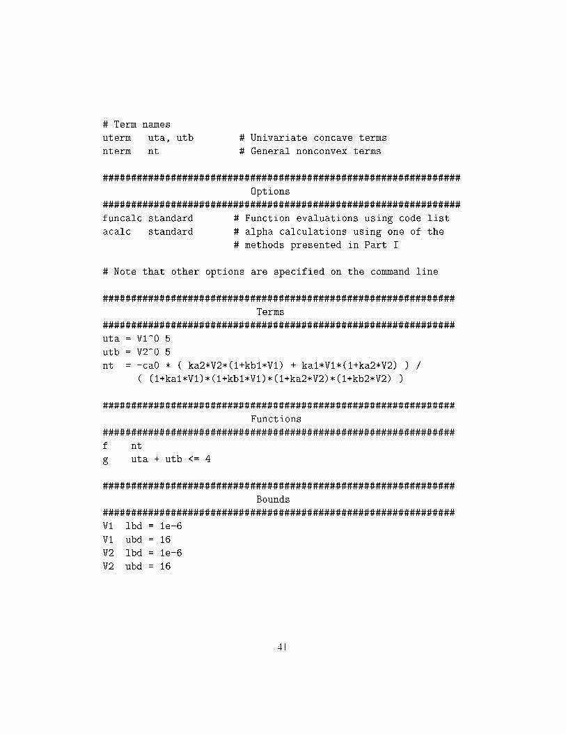
# Term namesuterm uta, utb # Univariate concave termsnterm nt # General nonconvex terms###############################################################Options###############################################################funcalc standard # Function evaluations using code listacalc standard # alpha calculations using one of the# methods presented in Part I# Note that other options are specified on the command line.##############################################################Terms##############################################################uta = V1^0.5utb = V2^0.5nt = -ca0 * ( ka2*V2*(1+kb1*V1) + ka1*V1*(1+ka2*V2) ) / \( (1+ka1*V1)*(1+kb1*V1)*(1+ka2*V2)*(1+kb2*V2) )##############################################################Functions##############################################################f .. ntg .. uta + utb <= 4##############################################################Bounds##############################################################V1 lbd = 1e-6V1 ubd = 16V2 lbd = 1e-6V2 ubd = 1641

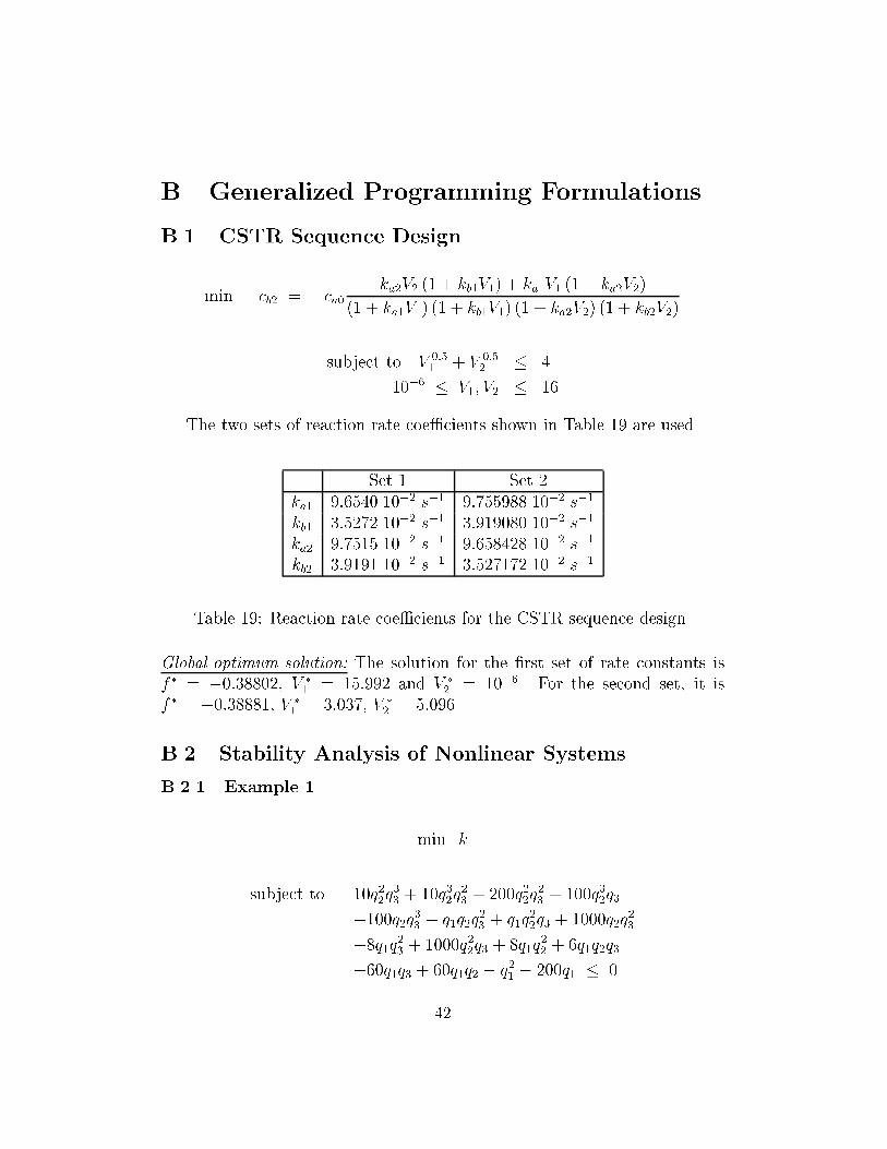
B Generalized Programming FormulationsB.1 CSTR Sequence Designmin �cb2 = �ca0 ka2V2 (1 + kb1V1) + ka1V1 (1 + ka2V2)(1 + ka1V1) (1 + kb1V1) (1 + ka2V2) (1 + kb2V2)subject to V 0:51 + V 0:52 � 410�6 � V1; V2 � 16The two sets of reaction rate coe�cients shown in Table 19 are used.Set 1 Set 2ka1 9:6540 10�2 s�1 9:755988 10�2 s�1kb1 3:5272 10�2 s�1 3:919080 10�2 s�1ka2 9:7515 10�2 s�1 9:658428 10�2 s�1kb2 3:9191 10�2 s�1 3:527172 10�2 s�1Table 19: Reaction rate coe�cients for the CSTR sequence designGlobal optimum solution: The solution for the �rst set of rate constants isf � = �0:38802, V �1 = 15:992 and V �2 = 10�6. For the second set, it isf � = �0:38881, V �1 = 3:037, V �2 = 5:096.B.2 Stability Analysis of Nonlinear SystemsB.2.1 Example 1 min ksubject to 10q22q33 + 10q32q23 + 200q22q23 + 100q32q3+100q2q33 + q1q2q23 + q1q22q3 + 1000q2q23+8q1q23 + 1000q22q3 + 8q1q22 + 6q1q2q3+60q1q3 + 60q1q2 � q21 � 200q1 � 042

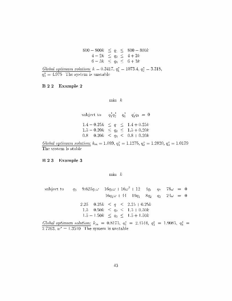
800� 800k � q1 � 800 + 800k4� 2k � q2 � 4 + 2k6� 3k � q3 � 6 + 3kGlobal optimum solution: k = 0:3417, q�1 = 1073:4, q�2 = 3:318,q�3 = 4:975. The system is unstable.B.2.2 Example 2 min ksubject to q41q42 � q41 � q42q3 = 01:4� 0:25k � q1 � 1:4 + 0:25k1:5� 0:20k � q2 � 1:5 + 0:20k0:8� 0:20k � q3 � 0:8 + 0:20kGlobal optimum solution: km = 1:089, q�1 = 1:1275, q�2 = 1:2820, q�3 = 1:0179.The system is stable.B.2.3 Example 3 min ksubject to q3 + 9:625q1! + 16q2! + 16!2 + 12� 4q1 � q2 � 78! = 016q1! + 44� 19q1 � 8q2 � q3 � 24! = 02:25� 0:25k � q1 � 2:25 + 0:25k1:5� 0:50k � q2 � 1:5 + 0:50k1:5� 1:50k � q3 � 1:5 + 1:50kGlobal optimum solution: km = 0:8175, q�1 = 2:4544, q�2 = 1:9085, q�3 =2:7263, w� = 1:3510. The system is unstable.43

B.2.4 Example 4 min ksubject to a4(q)!4 � a2(q)!2 + a0(q) = 0a3(q)!2 � a1(q) = 010:0� 1:0k � q1 � 10:0 + 1:0k1:0� 0:1k � q2 � 1:0 + 0:1k1:0� 0:1k � q3 � 1:0 + 0:1k0:2� 0:01k � q4 � 0:2 + 0:01k0:05� 0:005k � q5 � 0:05 + 0:005kwhere a4(q) = q23q2 (4q2 + 7q1)a3(q) = 7q4q23q2 � 64:918q23q2 + 380:067q3q2 + 3q5q2 + 3q5q1a2(q) = 3 ��9:81q3q22 � 9:81q3q1q2 � 4:312q23q2+264:896q3q2 + q4q5 � 9:274q5)a1(q) = 15 (�147:15q4q3q2 + 1364:67q3q2 � 27:72q5)a0(q) = 54:387q3q2Global optimum solution: k = 6:2746, q�1 = 16:2746, q�2 = 1:6275, q�3 =1:6275, q�4 = 0:1373, q�5 = 0:0186, w� = 0:9864. The system is stable.B.2.5 Example 5 min ksubject to a8(q)!8 � a6(q)!6 + a4(q)!4 � a2(q)!2 + a0(q) = 0a7(q)!6 � a5(q)!4 + a3(q)!2 � a1(q) = 017:5� 14:5k � q1 � 17:5 + 14:5k20:0� 15:0k � q2 � 20:0 + 15:0k44

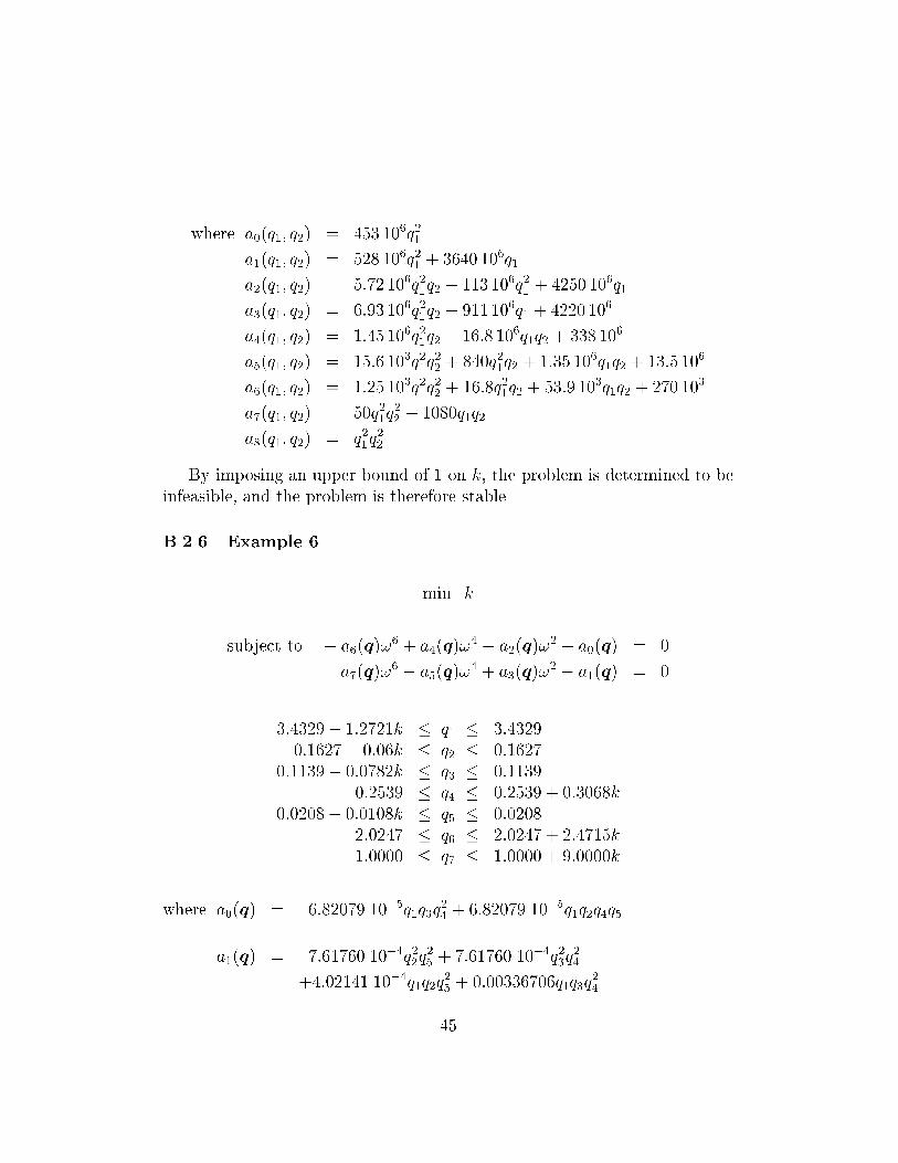
where a0(q1; q2) = 453 106q21a1(q1; q2) = 528 106q21 + 3640 106q1a2(q1; q2) = 5:72 106q21q2 + 113 106q21 + 4250 106q1a3(q1; q2) = 6:93 106q21q2 + 911 106q1 + 4220 106a4(q1; q2) = 1:45 106q21q2 + 16:8 106q1q2 + 338 106a5(q1; q2) = 15:6 103q21q22 + 840q21q2 + 1:35 106q1q2 + 13:5 106a6(q1; q2) = 1:25 103q21q22 + 16:8q21q2 + 53:9 103q1q2 + 270 103a7(q1; q2) = 50q21q22 + 1080q1q2a8(q1; q2) = q21q22By imposing an upper bound of 1 on k, the problem is determined to beinfeasible, and the problem is therefore stable.B.2.6 Example 6 min ksubject to � a6(q)!6 + a4(q)!4 � a2(q)!2 + a0(q) = 0a7(q)!6 � a5(q)!4 + a3(q)!2 � a1(q) = 03:4329� 1:2721k � q1 � 3:43290:1627� 0:06k � q2 � 0:16270:1139� 0:0782k � q3 � 0:11390:2539 � q4 � 0:2539 + 0:3068k0:0208� 0:0108k � q5 � 0:02082:0247 � q6 � 2:0247 + 2:4715k1:0000 � q7 � 1:0000 + 9:0000kwhere a0(q) = 6:82079 10�5q1q3q24 + 6:82079 10�5q1q2q4q5a1(q) = 7:61760 10�4q22q25 + 7:61760 10�4q23q24+4:02141 10�4q1q2q25 + 0:00336706q1q3q2445

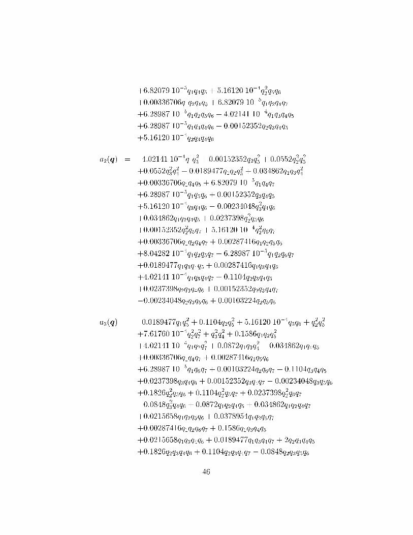
+6:82079 10�5q1q4q5 + 5:16120 10�4q22q5q6+0:00336706q1q2q4q5 + 6:82079 10�5q1q2q4q7+6:28987 10�5q1q2q5q6 + 4:02141 10�4q1q3q4q5+6:28987 10�5q1q3q4q6 + 0:00152352q2q3q4q5+5:16120 10�4q2q3q4q6a2(q) = 4:02141 10�4q1q25 + 0:00152352q2q25 + 0:0552q22q25+0:0552q23q24 + 0:0189477q1q2q25 + 0:034862q1q3q24+0:00336706q1q4q5 + 6:82079 10�5q1q4q7+6:28987 10�5q1q5q6 + 0:00152352q3q4q5+5:16120 10�4q3q4q6 � 0:00234048q23q4q6+0:034862q1q2q4q5 + 0:0237398q22q5q6+0:00152352q22q5q7 + 5:16120 10�4q22q6q7+0:00336706q1q2q4q7 + 0:00287416q1q2q5q6+8:04282 10�4q1q2q5q7 + 6:28987 10�5q1q2q6q7+0:0189477q1q3q4q5 + 0:00287416q1q3q4q6+4:02141 10�4q1q3q4q7 + 0:1104q2q3q4q5+0:0237398q2q3q4q6 + 0:00152352q2q3q4q7�0:00234048q2q3q5q6 + 0:00103224q2q5q6a3(q) = 0:0189477q1q25 + 0:1104q2q25 + 5:16120 10�4q5q6 + q22q25+7:61760 10�4q22q27 + q23q24 + 0:1586q1q2q25+4:02141 10�4q1q2q27 + 0:0872q1q3q24 + 0:034862q1q4q5+0:00336706q1q4q7 + 0:00287416q1q5q6+6:28987 10�5q1q6q7 + 0:00103224q2q6q7 + 0:1104q3q4q5+0:0237398q3q4q6 + 0:00152352q3q4q7 � 0:00234048q3q5q6+0:1826q22q5q6 + 0:1104q22q5q7 + 0:0237398q22q6q7�0:0848q23q4q6 + 0:0872q1q2q4q5 + 0:034862q1q2q4q7+0:0215658q1q2q5q6 + 0:0378954q1q2q5q7+0:00287416q1q2q6q7 + 0:1586q1q3q4q5+0:0215658q1q3q4q6 + 0:0189477q1q3q4q7 + 2q2q3q4q5+0:1826q2q3q4q6 + 0:1104q2q3q4q7 � 0:0848q2q3q5q646

�0:00234048q2q3q6q7 + 7:61760 10�4q25 + 0:0474795q2q5q6+8:04282 10�4q1q5q7 + 0:00304704q2q5q7a4(q) = 0:1586q1q25 + 4:02141 10�4q1q27 + 2q2q25 + 0:00152352q2q27+0:0237398q5q6 + 0:00152352q5q7 + 5:16120 10�4q6q7+0:0552q22q27 + 0:0189477q1q2q27 + 0:0872q1q4q5+0:034862q1q4q7 + 0:0215658q1q5q6 + 0:00287416q1q6q7+0:0474795q2q6q7 + 2q3q4q5 + 0:1826q3q4q6 + 0:1104q3q4q7�0:0848q3q5q6 � 0:00234048q3q6q7 + 2q22q5q7 + 0:1826q22q6q7+0:0872q1q2q4q7 + 0:3172q1q2q5q7 + 0:0215658q1q2q6q7+0:1586q1q3q4q7 + 2q2q3q4q7 � 0:0848q2q3q6q7 + 0:0552q25+0:3652q2q5q6 + 0:0378954q1q5q7 + 0:2208q2q5q7a5(q) = 0:0189477q1q27 + 0:1104q2q27 + 0:1826q5q6 + 0:1104q5q7+0:0237398q6q7 + q22q27 + 0:1586q1q2q27 + 0:0872q1q4q7+0:0215658q1q6q7 + 0:3652q2q6q7 + 2q3q4q7 � 0:0848q3q6q7+q25 + 7:61760 10�4q27 + 0:3172q1q5q7+4q2q5q7a6(q) = 0:1586q1q27 + 2q2q27 + 2q5q7 + 0:1826q6q7 + 0:0552q27a7(q) = q27By imposing an upper bound of 1 on k, the problem is determined to beinfeasible, and the problem is therefore stable.47