Differentiable SAT/ASP

Matthias Nickles

National University of Ireland, GalwaySchool of Engineering and Informatics

matthias.nickles@nuigalway.ie

Abstract. We propose Differentiable SAT and Differentiable Answer Set Pro-gramming for multi-model optimization through gradient-controlled answer setor satisfying assignment computation. As a use case, we also show how our ap-proach can be used for expressive probabilistic inference constrained by log-ical background knowledge. In addition to presenting an enhancement of theCDNL/CDCL algorithm as primary implementation approach, we introduce al-ternative algorithms which use an unmodified ASP solver and map the optimiza-tion task to conventional answer set optimization or use so-called propagators.

Keywords: SAT · ASP · Probabilistic Programming · Gradient Descent · Ap-proximate Probabilistic Inference · Relational Artificial Intelligence

1 Introduction

Modern SAT and Answer Set solvers are, like their closely related cousins constraintprocessing and Satisfiability Modulo Theories (SMT), powerful and fast tools for log-ical reasoning. We present an approach which utilizes and enhances current SAT/ASPsolving algorithms for multi-model optimization, with probabilistic inference as thefocused - but not the only - use case. We build on previous work [12] and add new al-gorithms, in particular methods which require only an existing, unmodified ASP solveror map the task to a regular answer set optimization problem.With Multi-model optimization we mean the search for a multi-set of models (satisfy-ing Boolean assignments or answer sets) which indirectly represents an (approximate)minimum of a user-provided cost function. We consider cost functions defined over cer-tain statistical properties of the model multi-set, namely frequencies of atoms (with costfunctions over fact, rule, clause or model weights as straightforward instances), and weincrementally sample models until a cost minimum is reached, with partial derivativesof the cost function guiding the assignment of decision literals in the SAT or ASP solv-ing process.In the use case of probabilistic logic programming (a form of declarative probabilisticprogramming), the resulting multi-model optimum approximates a probability distri-bution over possible worlds (models) induced by probabilistic constraints (encoded asthe cost function) and non-probabilistic rules and clauses (a regular ASP program orBoolean formula in CNF of which all sampled models are answer sets respectivelysatisfying assignments). By sampling only as many models as required for cost min-imization, we reduce the number of expensive conventional deductive inference steps

and avoid the combinatorial explosion of materialized possible worlds with increasingnumber of nondeterministic atoms which typically precludes the use of straightforwardoptimization techniques (such as linear programming) in probabilistic logic program-ming.In principle, arbitrary differentiable cost function can be used (although obviously notall cost functions lead to convergence of the optimization process) and there are no re-strictions on the background knowledge rules or clauses, or the random variables (suchas independence assumptions), except consistency. The expressiveness of the frame-work is thus quite high, and, despite the use of sampling, computation times remain achallenge (in particular in comparison with approaches which deliberately put restric-tions into place, such as frameworks based on the Distribution Semantics). We tacklethis concern with our first concrete algorithm (a variant of the algorithm presented in[12]) by integrating the cost minimization steps directly into a state-of-the-art ASP/SATsolving approach [4], and we compare its performance experimentally with that of sev-eral alternative methods introduced in this paper.The remainder of this paper is organized as follows: The following section introducesbasic concepts and notation. Sect. 3 presents our general approach and proposes severalconcrete computation methods. Sect. 4 presents results from preliminary experiments,and Sect. 5 discusses related approaches. Sect. 6 concludes.

2 Preliminaries

We consider ground normal logic programs under stable model semantics and SATproblems in form of propositional formulas in Conjunctive Normal Form (CNF). Re-call that a normal logic program is a finite set of rules of the formh :− b1, ..., bm, not bm+1, ..., not bn (with 0 ≤ m ≤ n). h and the bi are atoms withoutvariables. not represents default negation. Rules without body literals are called facts.Most other syntactic constructs supported by contemporary ASP solvers (like integrityconstraints, choice rules or classical negation) can be translated into (sets of) normalrules. We consider only ground programs in this work. The answer sets (stable mod-els) of a normal logic program are as defined in [5]. Throughout the paper, we use theterm “answer set program” to mean a ground normal logic program and “model” inthe sense of answer set or, in the SAT case, a complete truth assignment such that theformula evaluates to true, however, to use the same model notation with both ASP andSAT, we generally do not show false atoms in models, i.e., a model is represented asa set of atoms which hold in the model. As common in probabilistic ASP, we identifypossible worlds with models. ΨΥ denotes the set of all answer sets or satisfying assign-ments of answer set program or propositional formula Υ . Sometimes we use only logicprogramming terminology where the translation to SAT terminology is obvious (e.g.,“program” instead of set of clauses). The set of all atoms respectively propositionalvariables in a program or formula Υ is denoted as atoms(Υ ). We write S to denote aset of negative literals {si : si ∈ S}.A partial assignment denotes an incomplete “model under construction”: a sequence ofliterals which have been iteratively added (assigned) to the assignment (and sometimesretracted from the assignment in backtracking steps) by the SAT or ASP solver until the

assignment is complete or the procedure aborts in case of unsatisfiability.We use a unified approach to SAT and ASP solving based on nogoods [4] (correspond-ing to clauses in CNF, but with all literals negated; a concept originally introduced forconstraint solving). Clauses and rules are translated into nogoods in a preprocessingstep (covering Clark’s completion in the ASP case). Additional nogoods are learnedfrom conflicts and loops (in non-tight ASP programs).

2.1 Cost Functions and Parameter Atoms

The cost functions considered in this work are user-provided functions of several vari-ables. Each variable corresponds to a so-called parameter atom. When evaluating thecost function, we instantiate each variable with the normalized count (frequency) of therespective parameter atom in a possibly incomplete sample. The sample is a multi-setof models sampled with replacement from the complete set ΨΥ of answers sets of thegiven program, respectively the set of all satisfying assignments (SAT case). Wherea parameter atom or its negation can occur we speak of parameter literals. Parame-ter atoms can occur in rules and clauses of the given answer set program or Booleanformula without limitations, and may even be conditioned on the truth values of otheratoms, including other parameter atoms. The set of parameter atoms is denoted as θ or{θi}, and θi is the i-th parameter atom under some arbitrary but fixed order. We denotethe individual cost function variables corresponding to the parameter atoms as θvi or av

(where a is a parameter atom). The parameter atoms need to be chosen by the user fromthe overall set of atoms in the program or set of clauses (theoretically, all atoms couldbe declared parameter atoms, but this might be inefficient).With each newly sampled model, the frequencies of the parameter atoms are updatedas follows. β(sample) = 〈βsample(θ1), β

sample(θ2), ...〉 is defined as the (parameter)

frequencies vector 〈 |[mj : mj ∈ sample, θ1 ∈ mj ]||sample| , ...,

|[mj : mj ∈ sample, θn ∈ mj ]||sample| 〉

of parameter atom frequencies in the model multi-set sample . βsample(θi) denotes thefrequency of parameter atom θi in sample . We omit sample and simply write β(θi)where it is clear from the context what the sample is. cost(β(θ1), β(θ2), ...) evaluatesthe cost function cost over parameter frequencies vector β(sample). We sometimeswrite cost(sample) in place of cost(β(θ1), β(θ2), ...).It makes sense to allow only parameter atoms whose truth values are not fully fixed bythe input program or formula. To ensure this in the ASP case, we can give the logicprogram the shape of a so-called spanning program [13, 9] where uncertain atoms aare defined by spanning formulas: choice rules or analogous constructs amounting tonondeterministic facts 0{a}1 or (informally) a ∨ not a. However, our framework doesnot require any particular form of the input program or formula.Informal examples for cost functions are “In 30% of all models, atom a should holdand in 40% of all models, atom b should hold” or “Atom a should hold more often thanthe square root of the frequency of atom b minus 10%”. In principle, other types of costfunctions which refer to other properties of the current sample multi-set are conceivabletoo, provided the model sampler is able to minimize such a cost.

2.2 Cost Functions and Parameter Atoms for Probabilistic Logic Programming

For the application case of deductive probabilistic inference, cost functions specifyprobabilistic constraints, whereas the plain ASP rules or SAT clauses serve as hardconstraints. More concretely, we consider the case that the probabilistic constraints areprovided by the user in form of weights associated with individual parameter atoms θi.Weights directly represent probabilities. Weights can also be attached to arbitrary rules,by introducing weighted fresh auxiliary atoms as “shortcuts” for these rules, using thefollowing scheme: h :− b1, ..., bn, not aux and aux :− b1, ..., bn, not h [9].As one (but not the only) suitable cost function which can be derived directly from a setof weighted parameter atoms, we propose the use of the Mean Squared Error (MSE)cost(θv1 , θ

v2 , ...) :=

1n

∑ni=1(β(θi)−φi)2 (squared Euclidean distance normalized with

the number n of parameter atoms). The φi are the user-defined weights of the parameteratoms θi.With this cost function, appending models to the sample until the cost reaches zero(i.e., maximum accuracy) corresponds to finding a solution of a linear equation systemwith additional conditions to ensure that the solutions form a probability distribution,with the probabilities of all possible worlds ΨΥ as the unknowns and the actual modelfrequencies in sample as approximate solution vector (details are provided in [12]).Queries can then be performed as usual, by adding up the approximated probabilitiesof those possible worlds where the query holds (that is, the frequencies of those modelsin sample which positively contain the query atoms).As an example for how to assign probabilities to atoms using cost functions, considerfunction cost(av, bv) = ((0.2− av)2 +(0.6− bv)2)/2) which specifies that the weightof parameter atom a should be 0.2 and the weight of parameter atoms b should be 0.6.As another example, this time for a cost function different from MSE (but also solv-able using Differentiable ASP), consider cost(aux v, qv) = (0.4 − aux v/qv)2 whichspecifies that the conditional probability Pr(p|q) is 0.4. The accompanying answer setprogram needs to include rules aux :− p, q and p :− aux and q :− aux .

3 Differentiable SAT/ASP

To find a sample of models which minimizes the cost function, our approach iterativelyappends models to multi-set sample until the cost falls below a specified threshold(allowing the user to trade speed against accuracy). All models are answer sets or sat-isfying truth assignment of the given answer set program or Boolean formula, ensuringthat they adhere to the given “hard” logical constraints. Partial cost function derivativesguide, during the generation of each individual model, the SAT/ASP solving process onthe level of branching decisions, namely truth value assignments to parameter atoms.

Fig. 1(a) shows a high level view of this approach, named Differentiable SAT/ASPor ∂SAT/ASP for short. An outer loop (left side of Fig. 1(a)) samples models and addsthem to an initially empty multi-set sample until the termination criterion is reached(there are several specific possibility for checking termination, depending on the natureof the cost function and the use case: if the cost expression is not too large, we cancheck if it is equal or below a given threshold ψ (accuracy), and/or we could performa stagnation check on the cost or the parameter atom frequencies. In some applications

Fig. 1: Differentiable SAT/ASP (outline)

it might also be sensible to demand a minimum sample size n in addition to reach-ing threshold ψ, e.g., to increase the sample entropy). In our experiments, we simplystopped sampling when the cost reached or fell below ψ.The models are sampled with the aim of reducing the multi-model cost, using a formof discretized gradient descent. We approach this with a special branching rule for se-lecting decision literals (literals not enforced by propagation) for inclusion in the par-tial assignment: Each time the solver nondeterministically (i.e., not forced by rules orclauses) extends the partial assignment with a not yet assigned literal, the literal is se-lected from all unassigned parameter literals (if any) if the value (or its negation in caseof negative literals) of the cost function’s partial derivative with respect to this literalis minimal (compared with the values obtained for the other unassigned parameter lit-erals). Since the parameter search space is discrete, we could theoretically measure thecost impacts of hypothetically assignments of candidate literals directly. But taking thepartial derivatives with respect to the parameter atoms splits the overall cost calculation(which might be complex) into typically simpler calculations whose results can evenbe pre-computed and ranked after each new model according to their current values,after updating the frequencies vector β with the new model. Finally, for branching deci-sions on non-parameter decision literals, some conventional branching heuristics (e.g.,VSIDS) can be used.Fig. 1(b) outlines a variant where each new model is explicitly required to lower thecost, without specifying how to achieve this. A specific approach to this variant, pro-posed in [12], uses a so-called cost backtracking mechanism which in case a modelcandidate fails to improve the cost, jumps back to the most recent literal decision pointwith untried parameter literals and tries a new parameter literal. [12] also indicates howcost backtracking and a split of the set of parameter atoms into measured atoms andactual parameter atoms can be utilized for inductive weight learning and abductive rea-soning (which are not possible using the approach in Fig. 1(a)).In the following subsections, we propose concrete approaches to put the general ap-proach in Fig. 1(a) into practice.

3.1 Implementing Differentiable SAT/ASP based on CDNL

A concrete approach to the rather general scheme described above is to enhance thecurrent state-of-the-art approach to Answer Set Programming (Conflict-Driven No-good Learning (CDNL) [4]) or a similar approach (CDCL (Conflict-Driven ClauseLearning)- or DPLL-style solving) with a new branching rule which selects free pa-rameter literals for inclusion into the current partial assignment according to their neg-ative “impact” on the cost, determined using partial derivatives wrt. parameter atoms.This approach, which we call Diff-CDNL-ASP/SAT (as it covers both SAT and An-swer Set solving), is shown as Algo. 1. The SAT solving path through the algorithm,enabled by parameter SATmode , is largely identical to the more complex ASP path,with stable model checks and loop handling omitted. The algorithm is a variant of theapproach presented in [12], with a somewhat more general branching approach usingpartial derivatives but omitting the optional cost backtracking.Algo. 1 iteratively adds literals to a partial assignment until all literals are covered andno nogood is violated. Important steps are unit propagation, i.e., the deterministic ex-pansion of the partial assignment (procedure PROPAGATE) with literals “fired” by no-goods, and conflict analysis (conflict means at least one nogood is subset of the partialassignment) and handling, including the deriving of further nogoods from the analysisof conflicts and backjumping (undoing recent literal assignments) in line 21 (detailsfollow [4] and are omitted here for lack of space).The procedure for generating a single model (the while-loop from line 6) is thus guidedby the following factors: 1) the initial set of nogoods obtained from the CNF clauses orClark’s completion of the answer set program, 2) further nogoods added to this set byconflict handling or due to the presence of loops (ASP mode), 3) the given cost functionand set of parameter atoms, and 4) our new branching approach for assigning parameterliterals (lines 9 to 13). The inner while loop ends once all atoms are covered as posi-tive or negative literals (or UNSAT). Afterwards (line 25), the stable model check takesplace (unless in SAT mode), and the new model is appended to the multi-set sample .The outer loop (from line 3) ends when a convergence criterion is met (e.g., when thecost falls below the given accuracy threshold ψ (line 32) and we have obtained the re-quested number of models, or if there is no more progress).The decision branching rule is the main different to regular CDNL: In lines 11ff., weselect the next parameter literal according to the previously described approach usingpartial derivatives. At this, it was in all our initial tests sufficient for reaching conver-gence to fix a new ranking of parameter literals by the values of the respective partialderivatives only after a new model was generated (ignoring the current partial assign-ment in the computation of the parameter atom frequencies) and to use this ranking todetermine the next decision literal in line 11.For further details on the non-probabilistic aspects of the algorithm, we need to refer to[4] for lack of space. Note that for loop handling, Algo. 1 uses the older and simplerASSAT approach [10], just to simplify our initial implementation.

3.2 Differentiable ASP using propagators (Diff-ASP-ThProp)While the approach from Sect. 3.1 is quite fast (see Sect. 4), it has the shortcoming thatit cannot be realized using an unmodified existing ASP or SAT solver. As an alternative

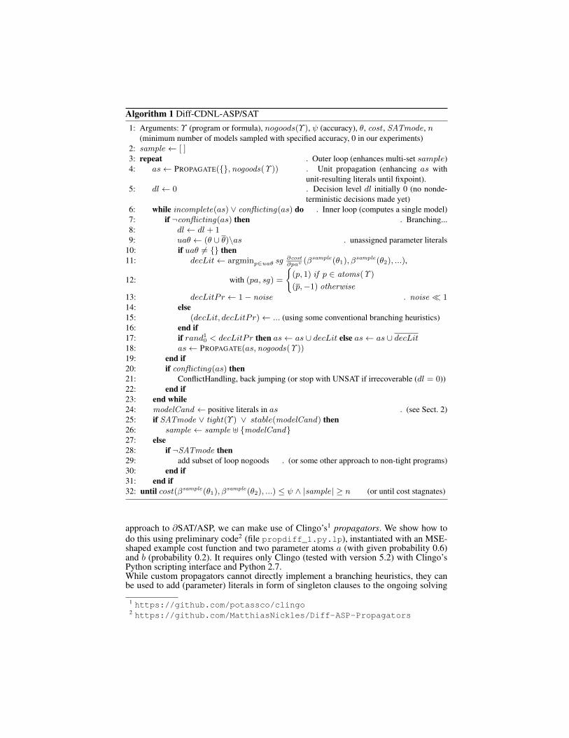
Algorithm 1 Diff-CDNL-ASP/SAT1: Arguments: Υ (program or formula), nogoods(Υ ), ψ (accuracy), θ, cost , SATmode , n

(minimum number of models sampled with specified accuracy, 0 in our experiments)2: sample ← [ ]3: repeat . Outer loop (enhances multi-set sample)4: as← PROPAGATE({},nogoods(Υ)) . Unit propagation (enhancing as with

unit-resulting literals until fixpoint).5: dl← 0 . Decision level dl initially 0 (no nonde-

terministic decisions made yet)6: while incomplete(as) ∨ conflicting(as) do . Inner loop (computes a single model)7: if ¬conflicting(as) then . Branching...8: dl← dl + 19: uaθ ← (θ ∪ θ)\as . unassigned parameter literals

10: if uaθ 6= {} then11: decLit← argminp∈uaθ sg ∂cost

∂pav(βsample(θ1), β

sample(θ2), ...),

12: with (pa, sg) =

{(p, 1) if p ∈ atoms(Υ)

(p,−1) otherwise

13: decLitPr ← 1− noise . noise � 114: else15: (decLit, decLitPr)← ... (using some conventional branching heuristics)16: end if17: if rand10 < decLitPr then as← as ∪ decLit else as← as ∪ decLit18: as← PROPAGATE(as,nogoods(Υ))19: end if20: if conflicting(as) then21: ConflictHandling, back jumping (or stop with UNSAT if irrecoverable (dl = 0))22: end if23: end while24: modelCand ← positive literals in as . (see Sect. 2)25: if SATmode ∨ tight(Υ ) ∨ stable(modelCand) then26: sample ← sample ] {modelCand}27: else28: if ¬SATmode then29: add subset of loop nogoods . (or some other approach to non-tight programs)30: end if31: end if32: until cost(βsample(θ1), β

sample(θ2), ...) ≤ ψ ∧ |sample| ≥ n (or until cost stagnates)

approach to ∂SAT/ASP, we can make use of Clingo’s1 propagators. We show how todo this using preliminary code2 (file propdiff_1.py.lp), instantiated with an MSE-shaped example cost function and two parameter atoms a (with given probability 0.6)and b (probability 0.2). It requires only Clingo (tested with version 5.2) with Clingo’sPython scripting interface and Python 2.7.While custom propagators cannot directly implement a branching heuristics, they canbe used to add (parameter) literals in form of singleton clauses to the ongoing solving

1 https://github.com/potassco/clingo2 https://github.com/MatthiasNickles/Diff-ASP-Propagators

process, intercepting propagation. We compute the parameter literal we would like toassign next (again using the approach in Sect. 3) and then pass this literal(branch_param_lit) on to the propagator (lines 56ff. in the code) to add it to thepartial assignment.The rest of the Python code is straightforward: The loop from line 155 corresponds tothe outer loop in Algo. 1: it iteratively calls the solver to compute new models, addseach newly sampled model to the model list sample (in callback on_model), updatesfrequencies and evaluates the cost (method update_cost), and checks for convergenceagainst threshold psi.The code supports both numerical and automatic differentiation (the latter using the adpackage3). In both cases, the search for the parameter literal which gives the minimumpartial derivative (i.e., steepest descent) is performed in lines 124ff. Automatic differen-tiation wrt. parameter atoms takes place in method __cost_ad. For numerical differen-tiation, we use a simple approximation which just adds a small value h to the frequencyof each respective parameter atom to estimate the slope (method__cost_upd).The actual cost function (including the given weights of the two parameter atoms) is inline 84 (we use the expression format of the ad-package for Python to represent the costexpression, also with numerical differentiation).(Remark: We have also experimented with domain heuristics using Clingo’s designatedpredicate _heuristic/3, but found no way yet to make this reliably working for ouruse case. Also, this attempt appears to be much slower than all other approaches pre-sented in this paper.)An example for a simple associated background theory (file propdiff_bgk_1.lp) is0{a}1. % spanning rule for parameter atom a0{b}1.:- a, b. % an example for a hard rule

The overall program is called with clingo-python propdiff_1.py.lp propdiff_bgk_1.lp

3.3 Direct cost minimization using model reification (Diff-ASP-Reification)

As the final approach proposed in this paper, we use Clingo with reified predicates andmodels to solve the cost function directly (without derivatives involved), alternativelyby mapping it to a conventional single answer set optimization task or by mapping theproblem to ASP-encoded equation solving.Here, each predicate in the original answer set program (not only the parameter atoms)whose truth value is not fully fixed is enhanced with a model number as extra argument.This way, we can let a single actual model (returned by Clingo) represent multiplereified models where each reified model consists exactly of those atoms in the actualmodel which share the same model number as their extra argument.We distinguish two flavors of this approach: 1) Computation of one or more individuallyoptimal answer set(s) using optimization statements or weak constraints (...:∼...), assupported by several ASP solvers, including smodels, DLV and Clingo/clasp, and 2)using ASP directly for constrained linear equations solving.We consider variant 1) first, shown in the code below for the same example as before(two uncertain atoms a and b with weights 0.2 and 0.6), and MSE as cost functionformat (adaptations to some other types of cost function should be straightforward). Thenumber of reified models nmodels does not need to be known precisely but shouldbe at least 10n where n is the number of decimal places which should be accurate

3 https://pypi.org/project/ad/

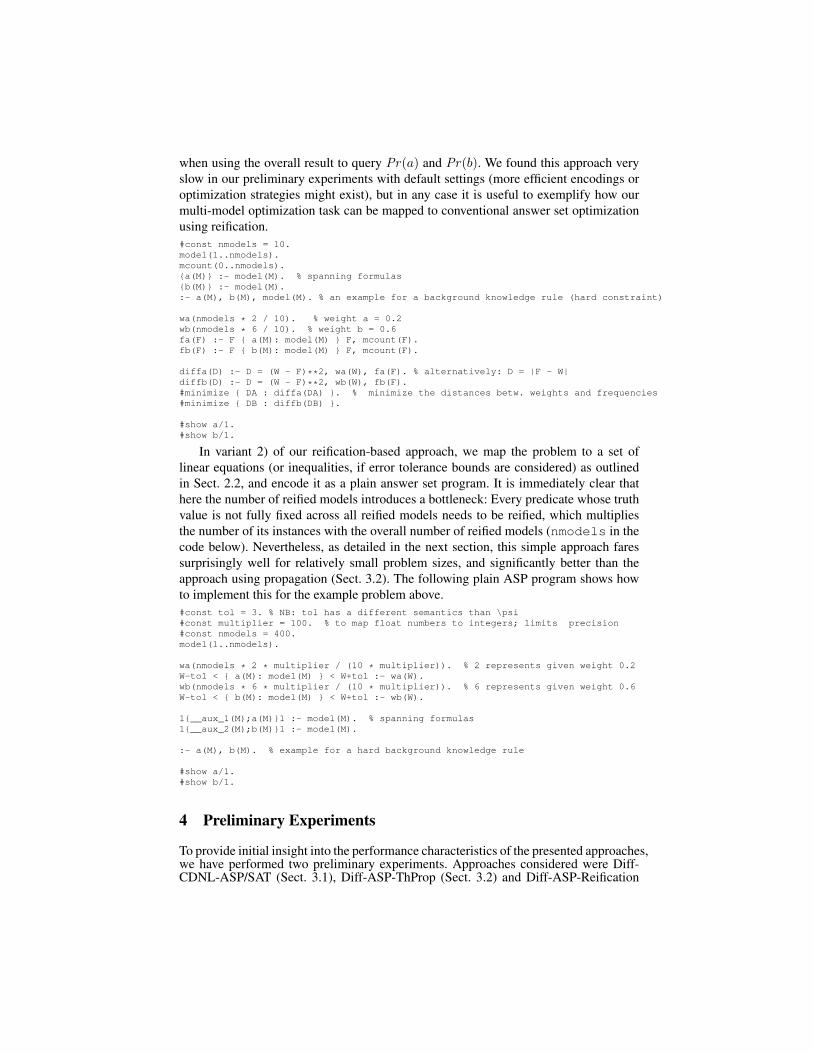
when using the overall result to query Pr(a) and Pr(b). We found this approach veryslow in our preliminary experiments with default settings (more efficient encodings oroptimization strategies might exist), but in any case it is useful to exemplify how ourmulti-model optimization task can be mapped to conventional answer set optimizationusing reification.#const nmodels = 10.model(1..nmodels).mcount(0..nmodels).{a(M)} :- model(M). % spanning formulas{b(M)} :- model(M).:- a(M), b(M), model(M). % an example for a background knowledge rule (hard constraint)

wa(nmodels * 2 / 10). % weight a = 0.2wb(nmodels * 6 / 10). % weight b = 0.6fa(F) :- F { a(M): model(M) } F, mcount(F).fb(F) :- F { b(M): model(M) } F, mcount(F).

diffa(D) :- D = (W - F)**2, wa(W), fa(F). % alternatively: D = |F - W|diffb(D) :- D = (W - F)**2, wb(W), fb(F).#minimize { DA : diffa(DA) }. % minimize the distances betw. weights and frequencies#minimize { DB : diffb(DB) }.

#show a/1.#show b/1.

In variant 2) of our reification-based approach, we map the problem to a set oflinear equations (or inequalities, if error tolerance bounds are considered) as outlinedin Sect. 2.2, and encode it as a plain answer set program. It is immediately clear thathere the number of reified models introduces a bottleneck: Every predicate whose truthvalue is not fully fixed across all reified models needs to be reified, which multipliesthe number of its instances with the overall number of reified models (nmodels in thecode below). Nevertheless, as detailed in the next section, this simple approach faressurprisingly well for relatively small problem sizes, and significantly better than theapproach using propagation (Sect. 3.2). The following plain ASP program shows howto implement this for the example problem above.#const tol = 3. % NB: tol has a different semantics than \psi#const multiplier = 100. % to map float numbers to integers; limits precision#const nmodels = 400.model(1..nmodels).

wa(nmodels * 2 * multiplier / (10 * multiplier)). % 2 represents given weight 0.2W-tol < { a(M): model(M) } < W+tol :- wa(W).wb(nmodels * 6 * multiplier / (10 * multiplier)). % 6 represents given weight 0.6W-tol < { b(M): model(M) } < W+tol :- wb(W).

1{__aux_1(M);a(M)}1 :- model(M). % spanning formulas1{__aux_2(M);b(M)}1 :- model(M).

:- a(M), b(M). % example for a hard background knowledge rule

#show a/1.#show b/1.

4 Preliminary Experiments

To provide initial insight into the performance characteristics of the presented approaches,we have performed two preliminary experiments. Approaches considered were Diff-CDNL-ASP/SAT (Sect. 3.1), Diff-ASP-ThProp (Sect. 3.2) and Diff-ASP-Reification

(Sect. 3.3), the latter in the equation solving variant (the version using #minimizeproved too slow with these experiments to be considered).We performed two synthetic experiments (Figs. 2a and 2b): a coin tossing game withbackground rules and a variant of the well-known “Friends & Smokers” scenario (whichexists in several variants in the literature). Times have been averaged over three trialsper experiment on a i7-4810MQ machine (4 cores, 2.8GHz) with 16GB RAM. TheDiff-CDNL variant of the ∂SAT/ASP approach (Sect. 3.1) has been experimentallyimplemented in Scala 2.12 (i.e., running in a Java VM). Experiments have been per-formed with different accuracy thresholds ψ. All times are end-to-end times, so theyinclude some overhead for file operations, parsing, etc. For the Clingo-based tasks wehave used Clingo 5.2.2 with Python 2.7.10 for scripting. The tolerance 20 specified withthe reification-based tasks with 400 models corresponds roughly to accuracy ψ ≈ .001for coins and ψ ≈ 0.05 for smokers.In the coin game, a number of coins are tossed and the game is won if a certain subsetof all coins comes up with “heads”. The inference task is the approximation of the win-ning probability, calculated by counting the models with the winning coin combinationswithin the resulting sample and normalizing this count with the size of the sample. Inaddition, another random subset of coins are magically dependent from each other andone of the coins is biased (probability of “heads” is 0.6). This scenario contains proba-bilistically independent as well as mutually dependent uncertain facts. Also, inferencedifficulty clearly scales with the number of coins. In pseudo-syntax, such a randomlygenerated program looks, e.g., as follows:coin(1..8).0.6: coin_out(1,heads).0.5: coin_out(N,heads) :- coin(N), N != 1.1{coin_out(N,heads), coin_out(N,tails)}1 :- coin(N).win :- 2{coin_out(3,heads),coin_out(4,heads)}2.coin_out(4,heads) :- coin_out(6,heads).

The proposed methods cannot directly work with non-ground rules, so weightednon-ground rules anywhere have been translated into sets of ground rules, each (re-spectively, their corresponding auxiliary “shortcut” parameter atoms) annotated withthe respective weights.In “Friends & Smokers”, a randomly chosen number of persons are friends, a ran-domly chosen subset of all people smoke, there is a certain probability for being stressed(0.3: stress(X)), it is assumed that stress leads to smoking (smokes(X) :- stress(X)),and that friends influence each other with a certain probability (0.2: influences(X,Y)),in particular with regard to smoking: smokes(X) :- friend(X,Y), influences(Y,X), smokes(Y).Smoking may leads to asthma (0.4: h(X). asthma(X) :- smokes(X), h(X)). The queryatoms are asthma(X) per each person X.For both experiments, it should be kept in mind that ∂SAT/ASP does not include anyspecial treatment of probabilistic independence.While the solution using Clingo with reified models cannot compete with the nativeapproach Diff-CDNL-ASP/SAT, it is still surprisingly fast, which, together with thefact that there is virtually no difference between the 400 and 800 model variants (thecurves almost cover each other), exemplifies the strong solving performance of Clingo.However, these results also seem to indicate (since both Clingo/clasp and Diff-CDNL-ASP/SAT are based on CDNL) that the prototypical Diff-CDNL-ASP/SAT implemen-tation could be made significantly faster by further optimizing its code or by using, e.g.,C/C++ or Rust. The alternative approach using propagators is clearly usable only fortiny problems, at least with the current implementation (the graph for Diff-ASP-ThPropwith ψ = 0.001 is not visible in Fig. 2a because its task immediately timed out).

(a) Coin Game (b) Friends & Smokers

Fig. 2: Preliminary performance results

5 Related Work

[2] proposes distribution-aware sampling for SAT with weight functions over entiremodels (which might be seen as an instance of our MSE-style variant of cost optimiza-tion, albeit technically approached very differently). Also related is the weighted satis-fiability problem which aims at maximizing the sum of the given weights of satisfiedclauses (e.g., using MaxWalkSAT [8]), which can be used for inference in Bayesiannetworks. PSAT (Probabilistic Boolean Satisfiability) [16] and SSAT problem [14]tackle related but different problems compared to ours. The envisaged main applica-tion case for our multi-model sampling approach is probabilistic logic (programming)and probabilistic deductive databases, in particular Probabilistic ASP (of which exist-ing approaches include, e.g., [1, 11, 9, 13]), but we expect other uses cases too, suchas working with combinatorial and search problems with uncertain facts and rules. Inthe context of nonmonotonic Probabilistic Inductive Logic Programming, gradient de-scent has been used for weight estimation. E.g., [3] uses gradient descent to estimatethe probabilities of abducibles. In contrast to the common MC-SAT sampling approachto inference with Markov Logic Networks (MLNs) [15] (a form of slice sampling),our task has a different semantics and our sampler is not wrapped around a uniformsampler, and we allow to specify rule or clause probabilities directly. An interesting ap-proach with combines MLN with logic programming under the stable model semanticsand compiles programs directly into ASP (using weak constraints) is [9]. Other than ourapproach, existing approaches to machine learning-based SAT solving (such as Learn-ing Rate Branching Heuristic (LRB)), or the combination of gradient descent / neuralnetwork-based techniques or numerical optimization with SAT (such as [17]) aim at animprovement of SAT solving itself (which is not our concern in this work), or enablesingle model optimization.

6 Conclusion

We have presented differentiation-based approaches to SAT and ASP multi-model com-putation which sample models in order to minimizes a custom cost function. Using cus-tomized cost functions and parameter atoms, our overall approach can be instantiated inorder to provide a tool for probabilistic logic programming. Building on existing work[12], we have presented an approach using a steepest descent method, an algorithmwhich utilizes Clingo’s propagators, and finally an approach (not differentiation-based)which maps the problem to plain answer set optimization. Planned work comprisesfurther experiments and the determination of formal convergence criteria.

References

1. Baral, C., Gelfond, M., Rushton, N.: Probabilistic reasoning with answer sets. Theory Pract.Log. Program. 9(1), 57–144 (2009)

2. Chakraborty, S., Fremont, D.J., Meel, K.S., Seshia, S.A., Vardi, M.Y.: Distribution-awaresampling and weighted model counting for SAT. In: Procs. 28th AAAI Conference on Arti-ficial Intelligence (AAAI). pp. 1722–1730 (July 2014)

3. Corapi, D., Sykes, D., Inoue, K., Russo, A.: Probabilistic rule learning in nonmonotonicdomains. In: Computational Logic in Multi-Agent Systems. pp. 243–258. Springer (2011)

4. Gebser, M., Kaufmann, B., Neumann, A., Schaub, T.: Conflict-driven answer set solving. In:Procs. of the 20th Int’l Joint Conf. on Artificial Intelligence (IJCAI’07) (2007)

5. Gelfond, M., Lifschitz, V.: The stable model semantics for logic programming. In: Proc. ofthe 5th Int’l Conference on Logic Programming. vol. 161 (1988)

6. Gomes, C.P., Sabharwal, A., Selman, B.: Near-uniform sampling of combinatorial spacesusing xor constraints. In: NIPS. pp. 481–488 (2006)

7. Gressler, A., Oetsch, J., Tompits, H.: Harvey: A system for random testing in asp. In: LogicProgramming and Nonmonotonic Reasoning. Springer (2017)

8. Kautz, H., Selman, B., Jiang, Y.: A general stochastic approach to solving problems with hardand soft constraints. In: The Satisfiability Problem: Theory and Applications. pp. 573–586.American Mathematical Society (1996)

9. Lee, J., Talsania, S., Wang, Y.: Computing lp using asp and mln solvers. Theory and Practiceof Logic Programming 17(5-6), 942–960 (2017)

10. Lin, F., Zhao, Y.: Assat: computing answer sets of a logic program by sat solvers. ArtificialIntelligence 157(1), 115 – 137 (2004), nonmonotonic Reasoning

11. Ng, R.T., Subrahmanian, V.S.: Stable semantics for probabilistic deductive databases. Inf.Comput. 110(1), 42–83 (1994)

12. Nickles, M.: Sampling-based sat/asp multi-model optimization as a framework for proba-bilistic inference. In: Procs. 28th International Conference on Inductive Logic Programming(ILP’18). Springer (2018 (to appear))

13. Nickles, M., Mileo, A.: A hybrid approach to inference in probabilistic non-monotonic logicprogramming. In: 2nd Int’l Workshop on Probabilistic Logic Programming (PLP’15) (2015)

14. Papadimitriou, C.H.: Games against nature. J. Comput. Syst. Sci. 31(2), 288–301 (1985)15. Poon, H., Domingos, P.: Sound and efficient inference with probabilistic and deterministic

dependencies. In: Procs. of AAAI’06. pp. 458–463. AAAI Press (2006)16. Pretolani, D.: Probability logic and optimization sat: The psat and cpa models. Annals of

Mathematics and Artificial Intelligence 43(1), 211–221 (Jan 2005)17. Selsam, D., Lamm, M., Bunz, B., Liang, P., de Moura, L., Dill, D.L.: Learning a SAT solver

from single-bit supervision. CoRR abs/1802.03685 (2018)