This article was downloaded by: [14.96.119.15]On: 12 December 2013, At: 01:25Publisher: Taylor & FrancisInforma Ltd Registered in England and Wales Registered Number: 1072954 Registeredoffice: Mortimer House, 37-41 Mortimer Street, London W1T 3JH, UK

Journal of Information and OptimizationSciencesPublication details, including instructions for authors andsubscription information:http://www.tandfonline.com/loi/tios20

Optimal control problem of a replicatorsystem on differentiable manifold withboundaryArnab Gupta a & Dilip Kumar Bhattacharya ba Department of Mathematics , Narula Institute of Technology ,Agarpara , Indiab Department of Pure Mathematics , University of Calcutta , IndiaPublished online: 15 Aug 2013.

To cite this article: Arnab Gupta & Dilip Kumar Bhattacharya (2013) Optimal control problem of areplicator system on differentiable manifold with boundary, Journal of Information and OptimizationSciences, 34:1, 29-46, DOI: 10.1080/02522667.2013.777175

To link to this article: http://dx.doi.org/10.1080/02522667.2013.777175

PLEASE SCROLL DOWN FOR ARTICLE

Taylor & Francis makes every effort to ensure the accuracy of all the information (the“Content”) contained in the publications on our platform. However, Taylor & Francis,our agents, and our licensors make no representations or warranties whatsoever as tothe accuracy, completeness, or suitability for any purpose of the Content. Any opinionsand views expressed in this publication are the opinions and views of the authors,and are not the views of or endorsed by Taylor & Francis. The accuracy of the Contentshould not be relied upon and should be independently verified with primary sourcesof information. Taylor and Francis shall not be liable for any losses, actions, claims,proceedings, demands, costs, expenses, damages, and other liabilities whatsoever orhowsoever caused arising directly or indirectly in connection with, in relation to or arisingout of the use of the Content.

This article may be used for research, teaching, and private study purposes. Anysubstantial or systematic reproduction, redistribution, reselling, loan, sub-licensing,systematic supply, or distribution in any form to anyone is expressly forbidden. Terms &

Conditions of access and use can be found at http://www.tandfonline.com/page/terms-and-conditions

Dow

nloa

ded

by [

14.9

6.11

9.15

] at

01:

25 1

2 D

ecem

ber

2013

*E-mail: arnab.math08@gmail.com†E-mail: dkb_math@yahoo.com

Optimal control problem of a replicator system on diff erentiable manifold with boundary

Arnab Gupta *

Department of MathematicsNarula Institute of TechnologyAgarparaIndia

Dilip Kumar Bhattacharya †`

Department of Pure MathematicsUniversity of CalcuttaIndia

AbstractThe paper discusses constrained optimal control problem of the functional on a repli-

cator system with restrictions in the domain of defi nition on the objective functional, in the

sense that the domain is an open manifold with boundary where the boundary is a diff er-

entiable variety.

Keywords: Diff erentiable manifold with boundary, Diff erentiable variety, Replicator system, Opti-mal control problem, Pontryagin’s maximum principle.AMS Subject Classifi cation Code [2010]: 51H25, 26A18, 49J15, 49K99.

1. Introduction

Optimal control problems are of two types - (i) when the restrictions

are only in the parameter domain and (ii) when the restrictions are in the

stable domain and also in the parameter domain. The necessary condition

of optimality type (i) is known as Pontryagin’s maximum principle [12],

similar conditions of optimality in type (ii) is given in [1, 2, 15]. So far as

type (i) optimal control problem are concerned, their applications in real

world problems and the corresponding analysis are found in [3, 4, 5]. But

Journal of Information & Optimization SciencesVol. 34 (2013), No. 1, pp. 29–46

© Taru Publications

Dow

nloa

ded

by [

14.9

6.11

9.15

] at

01:

25 1

2 D

ecem

ber

2013

30 A. GUPTA AND D. K. BHATTACHARYA

the realistic application for type (ii) is not done yet. In the paper we will

discuss type (ii) optimal control problem on a replicator system.

In biochemistry or biology there is one class of molecules, which

appeared one day during evolution, for which selfreplication is obliga-

tory. These molecules, of course, are the polynucleotides, the nucleic acid

or, later in evolution the genes. These molecules interact with each other

(rather the dynamics or selfreplication between two or more molecules

happens) in a reaction vessels called evolution reactor. The evolution reac-

tor is a kind of fl ow reactor which consists of reaction vessel and allows

for temperature and pressure control. Its walls are impermeable to the

self replicative units (biological macromolecules like polynucleotides-e.g.

phage RNA- bacteria or in principle, also higher organisms). Energy rich

material (food) is poured from the environment into the reactor. The deg-

radation products (waste) are removed steadily. In such a evolution reac-

tor, material support is so adjusted that the food concentration remains

constant in the reactor, the waste is drawn out by dilution fl ux. Mathe-

matically it means that ,x cii

n

1

==

/ if xi are the concentrations. So any dif-

ferential equation (preferably replicator type of equation) involving such

xi ‘s means that the state space is a n-simplex. This is why n-simplex is also

called a concentration simplex.

Study of replicator system on a n- simplex or on a concentration sim-

plex is important from experimental as well as theoretical point of view.

The experimental importance is well known in literature [13, 14]. The the-

oretical importance is also worth mentioning. The generalization of repli-

cator dynamics and its permanence criteria through diff erent techniques

(viz., vector optimization technique etc.) has also been studied in [9, 10].

The paper discusses type (ii) optimal control on a replicator system in the

sense that the objective functional is restricted on a certain domain or state

space. The domain is an open manifold with boundary where the bound-

ary is a diff erentiable variety.

The whole matter of the paper is divided into four main sections,

where section 1 is the introductory one. Section 2 gives the idea of dif-

ferentiable manifold with boundary and diff erentiable variety and con-

tains some results in this connection. In section 3, some ideas of replica-

tor dynamics are given. Also a constrained optimal control problem with

restrictions in the state space are given on the domain of defi nition of the

functional, in the sense that, the domain is an open manifold with dif-

ferentiable variety as its boundary. Finally, in section 4 we formulate a

model and its stability analysis around a feasible equilibrium of replicator

system. We shall also state a control-theoretic optimization of a functional

Dow

nloa

ded

by [

14.9

6.11

9.15

] at

01:

25 1

2 D

ecem

ber

2013

OPTIMAL CONTROL PROBLEM 31

of replicator dynamics and thus discusses a optimal steady state analysis

of the aforesaid model around a bionomic equilibrium.

2. Some known defi nitions and results [6]

Defi nition 2.1. A C ∞ manifold with boundary of dimension n is a Haus-

droff space M with countable basis of open sets and a diff erentiable struc-

ture x defi ned in the following manner: {( , )}Vx z= !a a a K consists of

family of open subsets Ua of M , each with homeomorphism of za onto

open subsets of { ( , , ....., ) , 0}H x x x x R xn n n n1 2! $= = (for some 0,n 2 an

integer) topologized as a subspace of Rn such that

(1) {( , )}U za a a Cover M.

(2) If {( , )}U za a a and {( , )}U zb b b are elements of ,x then & :1z z -ab

( ) ( )U U U U"+ +z za b b a ba are diff eomorphisms where ( )U U+za a b

and ( )U U+zb a b are open subsets of Hn .

(3) {( , )}U za a a is maximal with respect to property (1) and (2).

Defi nition 2.2. A diff erentiable variety in R 1n + is defi ned as (0) ,f 1-" ,

where :f R R"1n + is a diff erentiable function such that at each ,z M! the

matrix j[ ( )]f z, has rank one, 1,2, .....,j n= .

Theorem 2.3. A diff erentiable variety M in R 1n + is a diff erentiable manifold of dimension n.

Example 2.4. A 2-sphere ( , , ) : 1 0S z z z R z z z3 2 2 22!= + + - =1 2 3 1 2 3

" , is a dif-ferentiable variety in R3 and it is a manifold of dimension 2.

3. Some known ideas of replicator dynamics and constrained optimal control problem with restrictions in the state space

Defi nition 3.1. [13] Let

( , , ) : , 0 1 3S x x x x R x c x for i1 2 33

1

3c

i ii

3 ! $ # #= = ==

) 3/ . It is called

concentration simplex.

Dow

nloa

ded

by [

14.9

6.11

9.15

] at

01:

25 1

2 D

ecem

ber

2013

32 A. GUPTA AND D. K. BHATTACHARYA

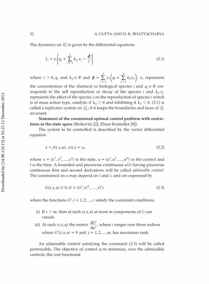
The dynamics on S3c is given by the diff erential equations

jx x q k xcj 1

3 z= + -

=i i ijio > H/ (3.1)

where 0,c q2 i and k R!ij and x q k xi i ij jji 1

3

1

3

z = +==

e o// . xi represents

the concentration of the chemical or biological species i and q R!i cor-

responds to the self reproduction or decay of the species i and jk xij

represents the eff ect of the species j on the reproduction of species i which

is of mass action type, catalytic if 0k 2ij and inhibiting if 0k 1ij . (3.1) is

called a replicator system on 3Sc ; if it keeps the boundaries and faces of 3S

c

invariant.

Statement of the constrained optimal control problem with restric-tions in the state space (Berkovitz [2], Elizer Kreindler [8]).

The system to be controlled is described by the vector diff erential

equation

( , , ), ( )x f t x u x t x= = 00o (3.2)

where ( , , ....., )x x x x1 2 n= is the state, ( , , ....., )u u u u1 2 m= is the control and t is the time. A bounded and piecewise continuous ( )u t having piecewise

continuous fi rst and second derivatives will be called admissible control. The constrained on u may depend on t and x, and are expressed by

( , , ) 0, ( , , .., )…G t x u G G G G1 2 r# = (3.3)

where the functions , 1,2, ....,G i ri = satisfy the constraint conditions:

(i) If ,r m2 then at each ( , , )t x u at most m components of G can

vanish.

(ii) At each ( , , )t x u the matrix u

Gj

i

2

2 , where i ranges over those indices

where ( , , ) 0G t x ui = and 1,2, ...., ,j m= has maximum rank.

An admissible control satisfying the constraint (3.3) will be called

permissible. The objective of control is to minimize, over the admissible

controls, the cost functional

Dow

nloa

ded

by [

14.9

6.11

9.15

] at

01:

25 1

2 D

ecem

ber

2013

OPTIMAL CONTROL PROBLEM 33

t

( ) ( , , )J u t x u dtt

r=1

0

# (3.4)

subject to (3.2) and (3.3), and some terminal conditions on ( )x t1 . For sim-

plicity, the terminal state and time will be fi xed given values

is fixed ( )t t x t t= =1 11 (3.5)

The functions ,π f and G are assumed to be twice continuously diff eren-

tiable in all arguments.

3.1. Optimal control problem

(I) Minimize over the admissible controls the cost functional (3.4)

subject to the diff erential equation (3.2), the constraint (3.3), and the termi-

nal condition (3.5).

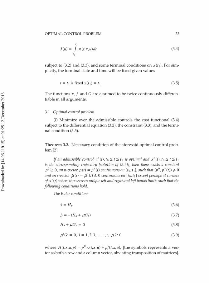
Theorem 3.2. Necessary condition of the aforesaid optimal control prob-

lem [2].

If an admissible control ( ),u t t t t# #0 1* is optimal and ( ),x t t t t# #0 1

*

is the corresponding trajectory [solution of (3.2)], then there exists a constant 0,p0

$ an n-vector ( ) ( )p t p t= * continuous on [ , ],t t0 1 such that ( , ( )) 0p p t0 * ! and an r-vector ( ) ( ) 0t t $n n= * continuous on [ , ]t t0 1 except perhaps at corners of ( )x t* where it possesses unique left and right and left hands limits such that the following conditions hold.

The Euler condition:

x H p=o (3.6)

( )p H Gx xn=- +o (3.7)

0H Gu un+ = (3.8)

0, 1,2,3, , , 0.……G i ri i$n n= = (3.9)

where ( , , , ) ( , , ) ( , , ),πH t x u p p t x u pf t x u0= + [the symbols represents a vec-

tor as both a row and a column vector, obviating transposition of matrices].

Dow

nloa

ded

by [

14.9

6.11

9.15

] at

01:

25 1

2 D

ecem

ber

2013

34 A. GUPTA AND D. K. BHATTACHARYA

The Weirstrass-Pontryagin’s condition:

For all permissible u (i.e., satisfying (3.3)) and for all [ , ],t t0 1

*( , , , ) ( , , , )H t x u p H t x u p#* ** (3.10)

In general we assume that the trajectory is normal i.e. 0p0 ! and can

be chosen as 1p0 = .

4. Model formulation, Stability analysis, Control-theoretic optimiza-tion of a functional of replicator dynamics and its optimal steady state analysis around bionomic equilibrium

In this section we prefer to restrict our detailed analysis only to the

following replicator system of dynamics, which is completely new in all

respects.

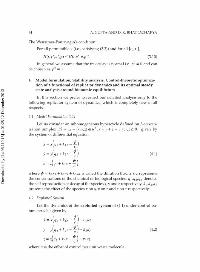
4.1. Model Formulation [11]

Let us consider an inhomogeneous hypercycle defi ned on 3-concen-

tration simplex ( , , ) : , , , 0S x x y z R x y z c x y z3c3 ! $= = + + =" , given by

the system of diff erential equation

x x q k yc

y y q k zc

z z q k xc

1 1

2 2

3 3

z

z

z

= + -

= + -

= + -

o

o

o

c

c

c

m

m

m

(4.1)

where k xy k yz k zxz = + +1 2 3 is called the dillution fl ux. , ,x y z represents

the concentrations of the chemical or biological species. 1, ,q q q2 3 denotes

the self reproduction or decay of the species x, y and z respectively. , ,k k k1 2 3

presents the eff ect of the species x on y, y on z and z on x respectively.

4.2. Exploited System

Let the dynamics of the exploited system of (4.1) under control pa-

rameter u be given by

x x q k yc

ux

y y q k zc

uy

z z q k xc

uz

1

zf

zf

zf

= + - -

= + - -

= + - -

1

2

1

3 3

2 2

3

o

o

o

c

c

c

m

m

m

(4.2)

where u is the eff ort of control per unit waste molecule.

Dow

nloa

ded

by [

14.9

6.11

9.15

] at

01:

25 1

2 D

ecem

ber

2013

OPTIMAL CONTROL PROBLEM 35

, ,1 2 3f f f : coeff icients of degradation product (waste) from evolution

reaction vessels for the molecules x, y and z respectively. In this case, the

state space of the dynamical system is a 3-simplex, which is actually a

manifold with boundary, the manifold being the open submanifold in R3

given by x y z c<+ + and the boundary being the diff erentiable variety

given by x y z c+ + = . The exploited system under the control parameter u is the 4-simplex , ,x y z u c u0 02#+ + + - which is also a manifold

with boundary; the interior is a 4- simplex

which is an open submanifold of R4 given by 0x y z u c 1+ + + -

and boundary is a 3-simplex x y z u c+ + + = .

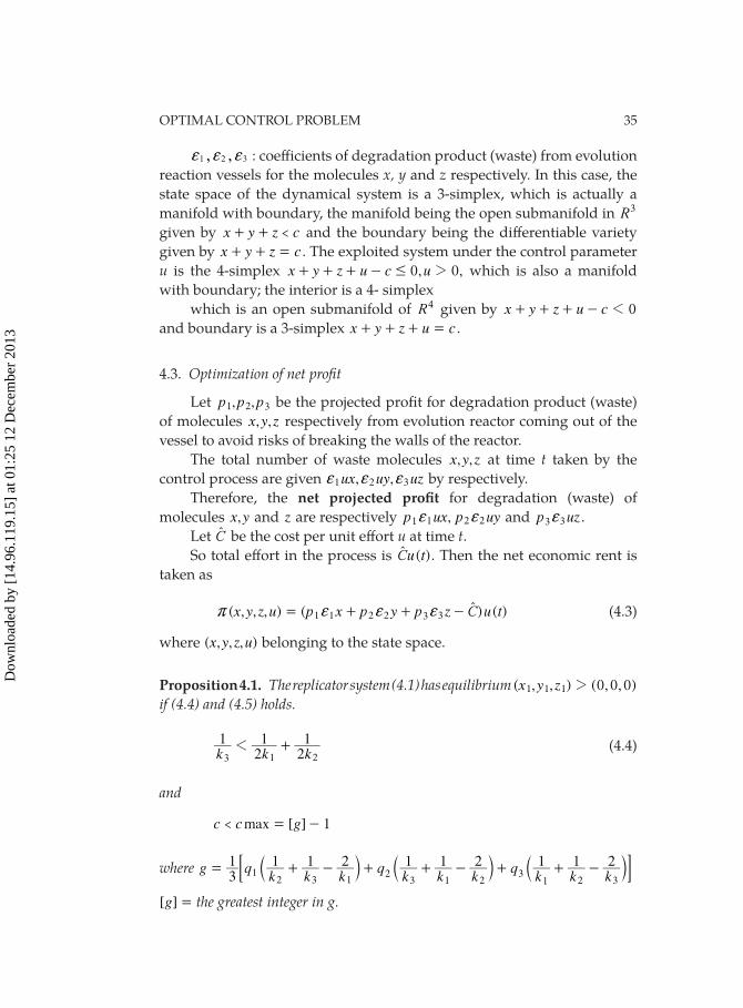
4.3. Optimization of net profi t

Let , ,p p p1 2 3 be the projected profi t for degradation product (waste)

of molecules , ,x y z respectively from evolution reactor coming out of the

vessel to avoid risks of breaking the walls of the reactor.

The total number of waste molecules , ,x y z at time t taken by the

control process are given , ,ux uy uz3f f f1 2 by respectively.

Therefore, the net projected profi t for degradation (waste) of

molecules ,x y and z are respectively ,p ux p uyf f1 2 21 and p uzf33 .

Let Ct be the cost per unit eff ort u at time t.So total eff ort in the process is ( )Cu tt . Then the net economic rent is

taken as

( , , , ) ( ) ( )x y z u p x p y p z C u tr f f f= + + -1 1 2 2 33t (4.3)

where ( , , , )x y z u belonging to the state space.

Proposition 4.1. The replicator system (4.1) has equilibrium ( , , ) (0,0,0)x y z 21 1 1 if (4.4) and (4.5) holds.

k k k1

21

211 +

1 23 (4.4)

and

[ ] 1maxc c g< = -

where 1 2g qk k k

qk k k

qk k k3

1 1 1 2 1 1 2 1 1 23 3

32

= + - + + - + + -2 1 1 2 31

b b bl l l: D

[ ]g = the greatest integer in g.

Dow

nloa

ded

by [

14.9

6.11

9.15

] at

01:

25 1

2 D

ecem

ber

2013

36 A. GUPTA AND D. K. BHATTACHARYA

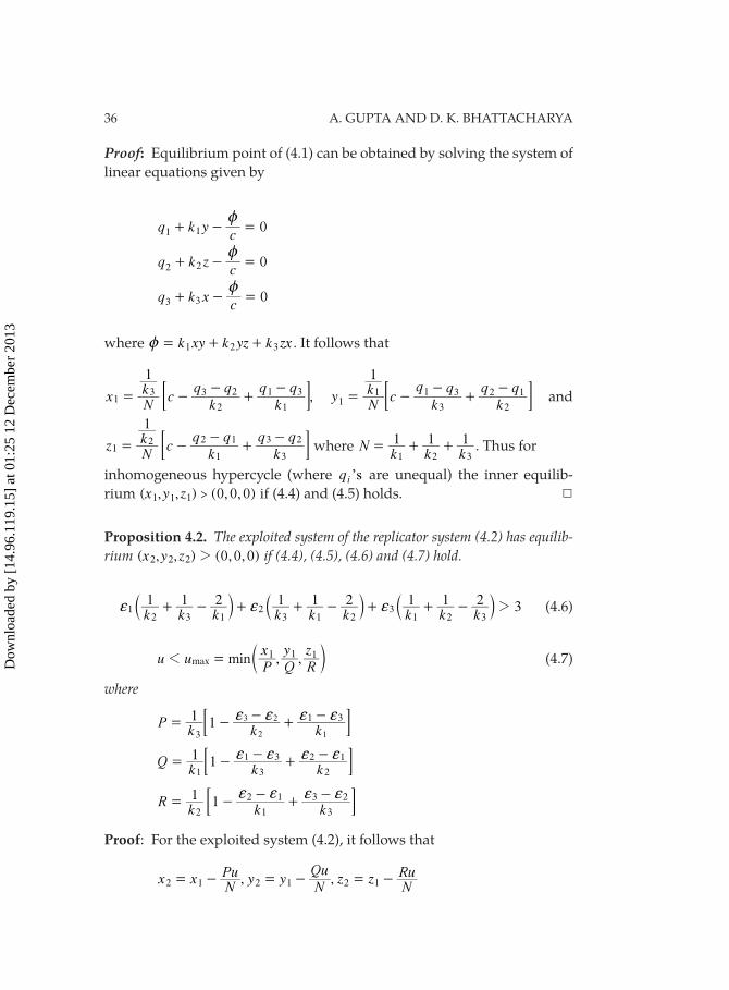
Proof: Equilibrium point of (4.1) can be obtained by solving the system of

linear equations given by

3

q k yc

q k zc

q k xc

0

0

0

1

2

3

z

z

z

+ - =

+ - =

+ - =

1

2

where k xy k yz k zxz = + +1 2 3 . It follows that

2 33 ,xNk

ck

q qk

q q1

13

2 1

1= --

+-

; E 3 1qy

Nk

ck

qk

q q11

3

1

2= -

-+

-21 ; E and

zNk

ck

q qk

q q1

12

1

2 1

3

3 2= -

-+

-; E where N

k k k1 1 11 2 3

= + + . Thus for

inhomogeneous hypercycle (where s’qi are unequal) the inner equilib-

rium ( , , ) (0,0,0)x y z >1 11 if (4.4) and (4.5) holds. 4

Proposition 4.2. The exploited system of the replicator system (4.2) has equilib-rium ( , , ) (0,0,0)x y z 22 2 2 if (4.4), (4.5), (4.6) and (4.7) hold.

3k k k k k k k k k1 1 2 1 1 2 1 1 2

12 3 1

23 1 2

31 2 3

2f f f+ - + + - + + -b b bl l l (4.6)

x z

, ,minu uP Q

yR

max11 = 11

c m (4.7)

where

Pk k k1 13

1 33 2f f f f= -

-+

-2 1

: D

Qk k k1 11 3

1 3

2

2 1f f f f= -

-+

-: D

f f f fR

k k k1 12 1

2 1

3

3 2= --

+-

: D

Proof: For the exploited system (4.2), it follows that

, ,x xNPu y y

NQu

z zNRu= - = - = -2 1 2 1 2 1

Dow

nloa

ded

by [

14.9

6.11

9.15

] at

01:

25 1

2 D

ecem

ber

2013

OPTIMAL CONTROL PROBLEM 37

where

f f

Pk k k1 1

2

2 f f= -

-+

-3

1

1 3

3: D

Qk k k1 1

3

3

2

2

1

1 1f f f f= -

-+

-: D

Rk k k1 1

3

3

2 1

2 1 2f f f f= -

-+

-: D

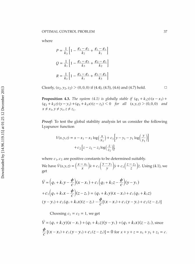
Clearly, ( , , ) (0,0,0)x y z 22 2 2 if (4.4), (4.5), (4.6) and (4.7) hold. 4

Proposition 4.3. The system (4.1) is globally stable if ( ) ( )q k y x x+ - +11 1 ( ) ( )q k z y y+ - +2 12 ( )( ) 0q k x z z 1+ -3 3 1 for all ( , , ) (0,0,0)x y z 2 and

,x x! 1 , .y y z z! !1 1

Proof: To test the global stability analysis let us consider the following

Lyapunov function

( , , ) log logV x y z x x xxx c y y y

yy

= - - + - -1 1 1 11

11

` cj m; E

,logc z z zzz

+ - -1

1 12 ` j8 B

where ,c c21 are positive constants to be determined suitably.

We have ( , , )V x y zx

x xx c

yy y

y cz

z zz1

11

2=-

+-

+- 1o o o ob c bl m l . Using (4.1), we

get

( ) ( )V q k y c x x c q k z c y y1 1 1 1 2 2 1

z z= + - - + + - -o c cm m

( )c q k x c z z2 3 3 1

z+ + - - =c m q k y x x c q k z1 1 1 1 2 2+ - + +^ ] ^h g h

y y c q k x z z1 2 3 3 1- + + -^ ^ ]h h g c x x c y y c z z1 1 1 2 1

z- - + - + -] ^ ]g h g6 @

Choosing 21 1,c c= = we get

( ) ( )V q k y x x q k z y y1 1 1 2 2 1= + - + + -o ^ ^h h ( )q k x z z3 3 1+ + -^ h , since

c x x c y y c z z 01 1 1 2 1

z- + - + - =] ^ ]g h g6 @ for x y z x y z c+ + = + + =1 1 1 .

Dow

nloa

ded

by [

14.9

6.11

9.15

] at

01:

25 1

2 D

ecem

ber

2013

38 A. GUPTA AND D. K. BHATTACHARYA

Thus by LaSalle’s theorem it follows that ( , , )x y z1 1 1 for the system (4.1)

is globally asymptotically stable if 1( )( ) ( )( )q k y x x q k z y y+ - + + -1 11 2 2

( )( ) 0q k x z z 1+ + -3 13 for all ( , , )x y z 02 and , ,x x y y z z! !! 1 1 1 . 4

In the similar manner it can be shown that 2( , , )x y z2 2 is globally

asymptotically stable.

4.4. Bionomic Equilibrium and its feasibility [7]

Let L denote the locus of dynamic equilibrium of the dynamic model

(4.2) and let 0r = denote the zero profi t function. A feasible equilibrium

is the point of intersection of 0L = and 0,r = provided all the coordi-

nates of this point are positive and also the value of the control parameter

u(t) is positive at this point. It is usually denoted by ( , , )x y z∞ ∞ ∞ .

The optimal steady state analysis is taken around the bionomic equi-

librium of the model, so its existence is to be assured. In this connection

we prove the following theorem.

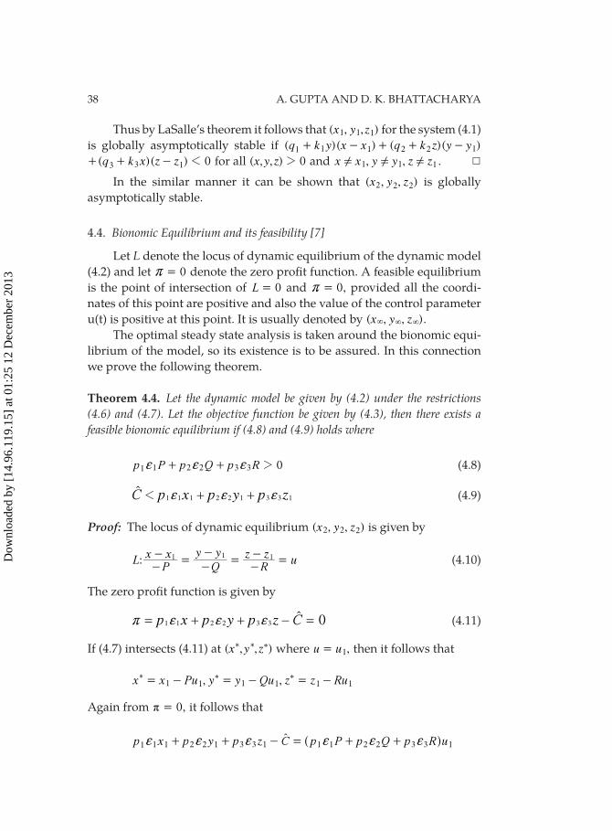
Theorem 4.4. Let the dynamic model be given by (4.2) under the restrictions (4.6) and (4.7). Let the objective function be given by (4.3), then there exists a feasible bionomic equilibrium if (4.8) and (4.9) holds where

0p P p Q p R1 1 2 3 2f f f+ +2 3 (4.8)

C p x p y p z1 1 1 2 2 1 3 3 11 f f f+ +t (4.9)

Proof: The locus of dynamic equilibrium ( , , )x y z2 2 2 is given by

1:LP

x xQ

y yR

z zu

1 1

--

=--

=--

= (4.10)

The zero profi t function is given by

p x p y p z C 01 1 2 2 3 3r f f f= + + - =t (4.11)

If (4.7) intersects (4.11) at ( , , )x y z* ** where ,u u= 1 then it follows that

, ,x x Pu y y Qu z z Ru= - = - = -1 1*

1 1 1* *

1

Again from 0,π = it follows that

p x p y p z C p P p Q p R u1 1 3 1 2f f f f f f+ + - = + +1 1 2 2 3 1 1 2 3 3 1t ] g

Dow

nloa

ded

by [

14.9

6.11

9.15

] at

01:

25 1

2 D

ecem

ber

2013

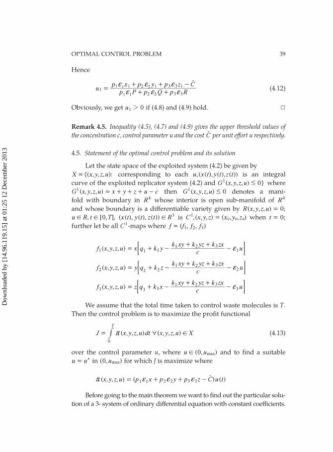
OPTIMAL CONTROL PROBLEM 39

Hence

2

2

2

2up P p Q p R

p x p y p z C1

31 1 1 1

1 1

1

f f ff f f

=+ +

+ + -

3 3

3t

(4.12)

Obviously, we get 0u 21 if (4.8) and (4.9) hold. 4

Remark 4.5. Inequality (4.5), (4.7) and (4.9) gives the upper threshold values of the concentration c, control parameter u and the cost Ct per unit eff ort u respectively.

4.5. Statement of the optimal control problem and its solution

Let the state space of the exploited system (4.2) be given by

{( , , , ): X x y z u= corresponding to each , ( ( ), ( ), ( ))u x t y t z t is an integral

curve of the exploited replicator system (4.2) and ( , , , ) } G x y z u 01# where

( , , , )G x y z u x y z u c1 = + + + - then ( , , , ) 0G x y z u1# denotes a mani-

fold with boundary in R4 whose interior is open sub-manifold of R4

and whose boundary is a diff erentiable variety given by ( , , , ) 0;R x y z u =

, [0, ],u R t T! ! ( ( ), ( ), ( ))x t y t z t R3! is 0, ( , , ) ( , , )C x y z x y z= 0

10 when 0;t =

further let be all C1-maps where ( , , )f f f f= 1 2 3

11 2

1( , , , )f x y z u x q k yc

k xy k yz k zxuf= + -

+ +-3

11 ; E

2

12

22( , , , )f x y z u q k

ck xy k yz k zx

uy z f= + -+ +

-32 ; E

13

233

( , , , )f x y z u q k xc

k xy k yz k zxuz f= + -

+ +-3

3 ; E

We assume that the total time taken to control waste molecules is T.

Then the control problem is to maximize the profi t functional

( , , , ) ( , , , )J x y z u dt x y z u X

T

0

6 !r= # (4.13)

over the control parameter u, where (0, )u u! max and to fi nd a suitable

u u= * in (0, )umax for which J is maximize where

3( , , , ) ( ) ( )x y z u p x p y p z C u tr f f f= + + -2 2 31 1t

Before going to the main theorem we want to fi nd out the particular solu-

tion of a 3- system of ordinary diff erential equation with constant coeff icients.

Dow

nloa

ded

by [

14.9

6.11

9.15

] at

01:

25 1

2 D

ecem

ber

2013

40 A. GUPTA AND D. K. BHATTACHARYA

Such solution of diff erential equation in co-state variable will be necessary

in our subsequent realistic example.

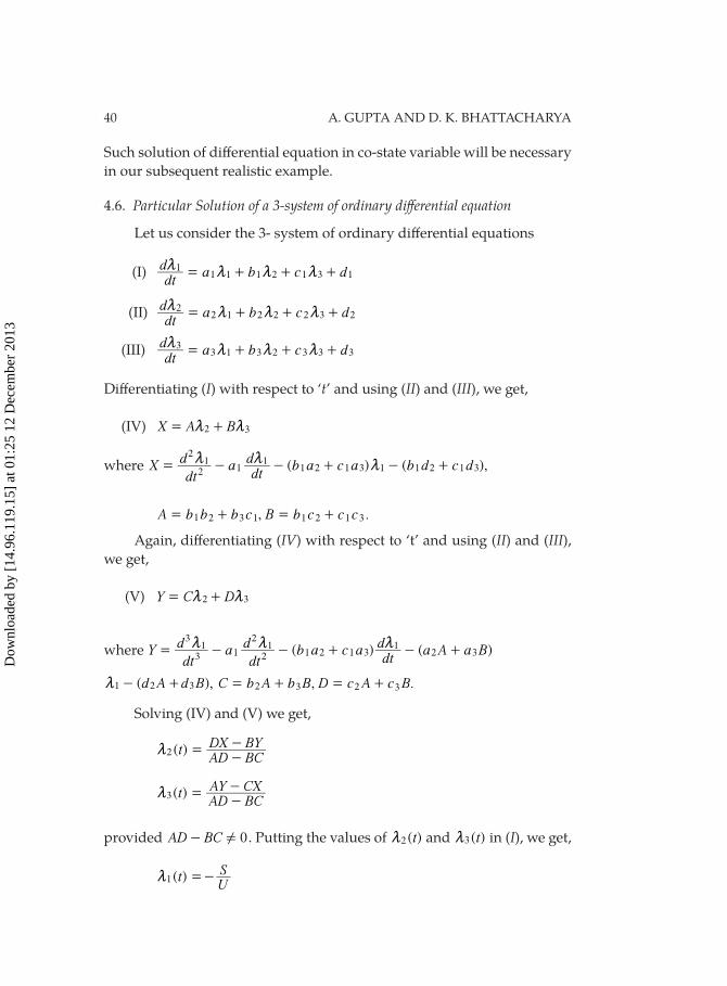
4.6. Particular Solution of a 3-system of ordinary diff erential equation

Let us consider the 3- system of ordinary diff erential equations

(I) dt

da b c d1

1 1 1 2 1 3 1m m m m= + + +

(II) dt

da b c d2

2 1 2 2 2 3 2m m m m= + + +

(III) dt

da b c d3

3 1 3 2 3 3 3m m m m= + + +

Diff erentiating (I) with respect to ‘t’ and using (II) and (III), we get,

(IV) X A B2m m= + 3

where ( ) ( ),Xdt

da

dtd

b a c a b d c d2

21

11

1 2 1 3 1 1 2 1 3m m m= - - + - +

, .A b b b c B b c c c= + = +1 2 3 1 1 2 1 3

Again, diff erentiating (IV) with respect to ‘t’ and using (II) and (III), we get,

(V) Y C D 3m m= +2

where ( ) ( )Ydt

da

dt

db a c a

dtd

a A a B3

31

1 2

21

1 2 1 31

2 3m m m

= - - + - +

(d A1 2m - + ),d B3 2 3, .C b A b B D c A c B= + = +2 3

Solving (IV) and (V) we get,

( )tAD BCDX BY

2m =--

( )tAD BCAY CX

3m =--

provided 0AD BC !- . Putting the values of ( )tm2 and ( )t3m in (I), we get,

( )tUS

1m =-

Dow

nloa

ded

by [

14.9

6.11

9.15

] at

01:

25 1

2 D

ecem

ber

2013

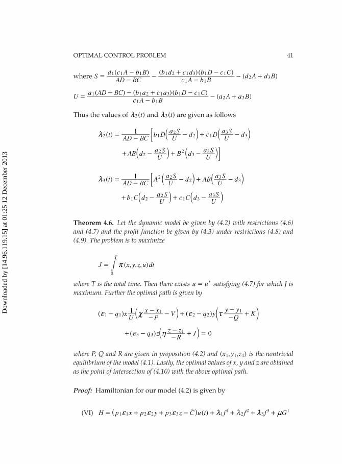
OPTIMAL CONTROL PROBLEM 41

where ( ) ( )( )

( )SAD BC

d c A b Bc A b B

b d c d b D c Cd A d B

1 1 1

1 1

1 2 1 3 1 12 3=

--

--

+ -- +

( ) ( )( )( )U

c A b Ba AD BC b a c a b D c C

a A a B1 1

1 1 2 1 3 1 12 3=

-- - + -

- +

Thus the values of ( )t2m and ( )t3m are given as follows

( )tAD BC

b DU

a Sd c D

Ua S

d12 1

22 1

33m =

-- + -b bl l;

AB dU

a SB d

Ua S

22 2

33+ - + -b bl lE

( )tAD BC

AU

a Sd AB

Ua S

d13

2 22

33m =

-- + -b bl l;

b C dU

a Sc C d

Ua S

1 22

1 33+ - + -b bl l

Theorem 4.6. Let the dynamic model be given by (4.2) with restrictions (4.6) and (4.7) and the profi t function be given by (4.3) under restrictions (4.8) and (4.9). The problem is to maximize

( , , , )J x y z u dt

T

0

r= #

where T is the total time. Then there exists u u= * satisfying (4.7) for which J is maximum. Further the optimal path is given by

q xU P

x xV q y

Qy y

K11 1

12 2

1f | f x---

- + ---

+] b ] cg l g m

0q zR

z zJ3 3

1f h+ ---

+ =] bg l

where P, Q and R are given in proposition (4.2) and ( , , )x y z1 1 1 is the nontrivial equilibrium of the model (4.1). Lastly, the optimal values of x, y and z are obtained as the point of intersection of (4.10) with the above optimal path.

Proof: Hamiltonian for our model (4.2) is given by

(VI) ( )H p x p y p z C u t f f f G1 1 2 2 3 3 11

22

33 1f f f m m m n= + + - + + + +t^ h

Dow

nloa

ded

by [

14.9

6.11

9.15

] at

01:

25 1

2 D

ecem

ber

2013

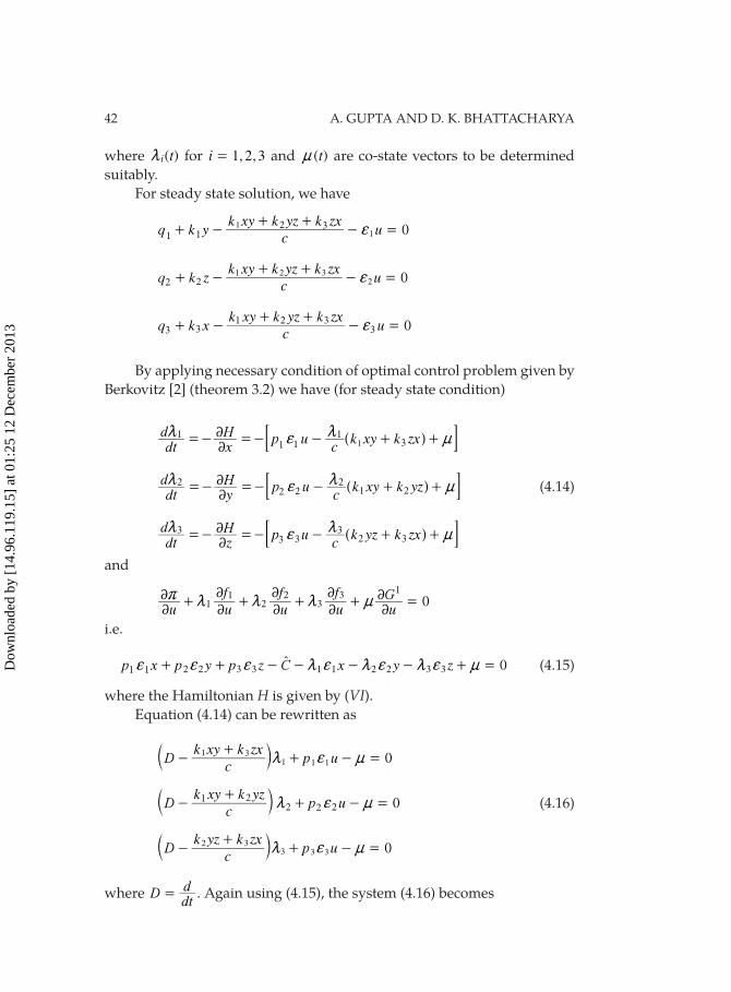
42 A. GUPTA AND D. K. BHATTACHARYA

where ( )tmi for 1,2,3i = and ( )tn are co-state vectors to be determined

suitably.

For steady state solution, we have

3 0q k yc

k xy k yz k zxu1f+ -

+ +- =1 2

11

21 3

2 0q k zc

k xy k yz k zxuf+ -

+ +- =2

2

13 3

33 0q k x

ck xy k yz k zx

u2 f+ -+ +

- =

By applying necessary condition of optimal control problem given by

Berkovitz [2] (theorem 3.2) we have (for steady state condition)

11 31dtd

xH p u

ck xy k zx1 1

22m f m n=- =- - + +] g: D

2 1 22dtd

yH p u

ck xy k yz2 2

22m f m n=- =- - + +] g: D (4.14)

3 2 3dtd

zH p u

ck yz k zx3 3

22m f m n=- =- - + +3 ] g: D

and

0u u

fuf

uf

uG

11

22

33

1

22

22

22

22

22r m m m n+ + + + =

i.e.

1 3 0p x p y p z C x y z3 2f f f m f m f m f n+ + - - - - + =2 2 1 1 2 3 31t (4.15)

where the Hamiltonian H is given by (VI).Equation (4.14) can be rewritten as

0Dc

k xy k zxp um f n-

++ - =

1 31 1 1b l

12 0D

ck xy k yz

p um f n-+

+ - =22 2b l (4.16)

0Dc

k yz k zxp u3m f n-

++ - =2 3

3 3b l

where Ddtd= . Again using (4.15), the system (4.16) becomes

Dow

nloa

ded

by [

14.9

6.11

9.15

] at

01:

25 1

2 D

ecem

ber

2013

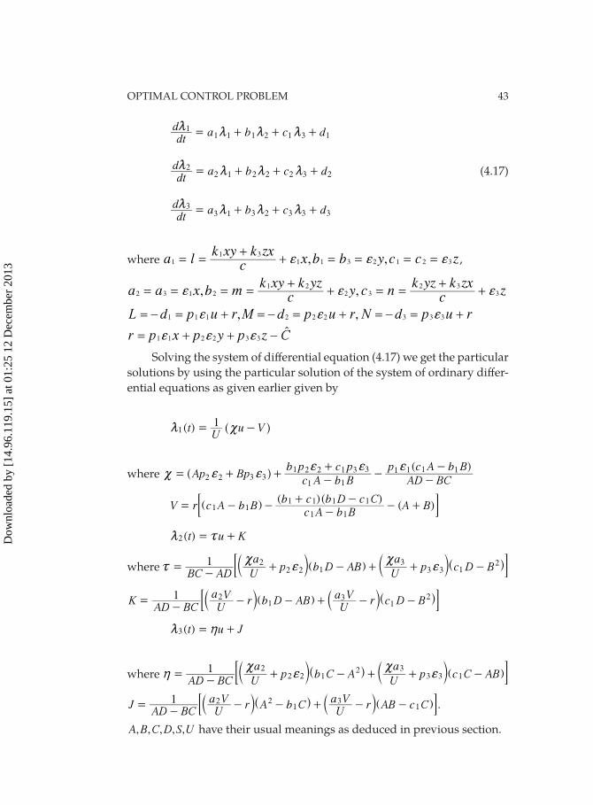
OPTIMAL CONTROL PROBLEM 43

1 1dtd

a b c d11

m m m m= + + +1 1 2 3

22 3 2dtd

a b c d21

m m m m= + + +2 2 (4.17)

33 3 3dtd

a b c d33 2

m m m m= + + +1

where , ,a l ck xy k zx

x b b y c c z11 3

1 1 3 2 1 2 3f f f= =+

+ = = = = ,

, ,a a x b m ck xy k yz

y c n ck yz k zx

z2 3 1 21 2

2 32 3

3f f f= = = =+

+ = =+

+

, ,L d p u r M d p u r N d p u r1 1 1 2 2 2 3 3 3f f f=- = + =- = + =- = +

r p x p y p z C1 1 2 2 3 3f f f= + + - t

Solving the system of diff erential equation (4.17) we get the particular

solutions by using the particular solution of the system of ordinary diff er-

ential equations as given earlier given by

( )tU

u V11m |= -^ h

where 321

33

3 11 ( )Ap Bp

c A b Bb p c p

AD BCp c A b B

1

1 1| f ff f f

= + +-+

--

-1 2 2 12] g

( )( )

( )V r c A b Bc A b B

b c b D c CA B1 1

1 1

1 1 1 1= - -

-+ -

- +] g; E

( )t u K2m x= +

where 112

23

BC AD U

ap b D AB

U

ap c D B1

32x

|f

|f=

-+ - + + -2 3c ] c ^m g m h; E

13a

KAD BC U

Vr b D AB

Ua V

r c D B1 21

2=-

- - + - -b ] b ^l g l h: D

( )t u J3m h= +

where AD BC U

ap b C A

U

ap c C AB1 2

2 2 12 3

3 3 1h|

f|

f=-

+ - + + -c ^ c ]m h m g; E

JAD BC U

a Vr A b C

Ua V

r AB c C1 2 21

31=

-- - + - -b ^ b ]l h l g: D.

, , , , ,A B C D S U have their usual meanings as deduced in previous section.

Dow

nloa

ded

by [

14.9

6.11

9.15

] at

01:

25 1

2 D

ecem

ber

2013

44 A. GUPTA AND D. K. BHATTACHARYA

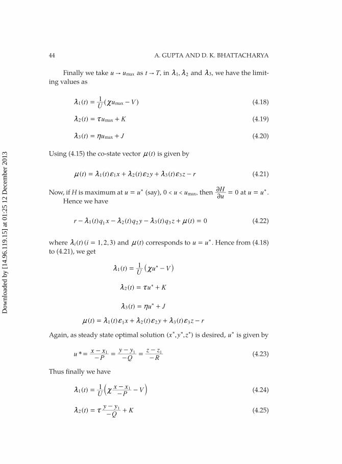
Finally we take u umax" as ,t T" in ,m m1 2 and ,3m we have the limit-

ing values as

( )tU

u V1max1m |= -^ h (4.18)

( )t u Kmax2m x= + (4.19)

( )t u Jmax3m h= + (4.20)

Using (4.15) the co-state vector ( )tn is given by

( ) ( ) ( ) ( )t t x t y t z r1 1 2 2 3 3n m f m f m f= + + - (4.21)

Now, if H is maximum at u u= * (say), 0 ,u u< < max then uH 022 = at u u= * .

Hence we have

1 2 3( ) ( ) ( ) ( ) 0r t q x t q y t q z t1 3m m m n- - - + =2 (4.22)

where ( ) ( 1,2,3)t im =i and ( )tn corresponds to u u= * . Hence from (4.18)

to (4.21), we get

( )tU

u V11m |= -*_ i

( )t u K2m x= +*

*( )t u J3m h= +

( ) ( ) ( ) ( )t t x t y t z r2 3n m f m f m f= + + -1 2 31

Again, as steady state optimal solution ( , , )x y z* * * is desired, u* is given by

*uP

x xQ

y yR

z z1 1 1=--

=--

=--

(4.23)

Thus fi nally we have

( )tU P

x xV1

11m |=

--

-b l (4.24)

( )tQ

y yK2m x=

--

+1 (4.25)

Dow

nloa

ded

by [

14.9

6.11

9.15

] at

01:

25 1

2 D

ecem

ber

2013

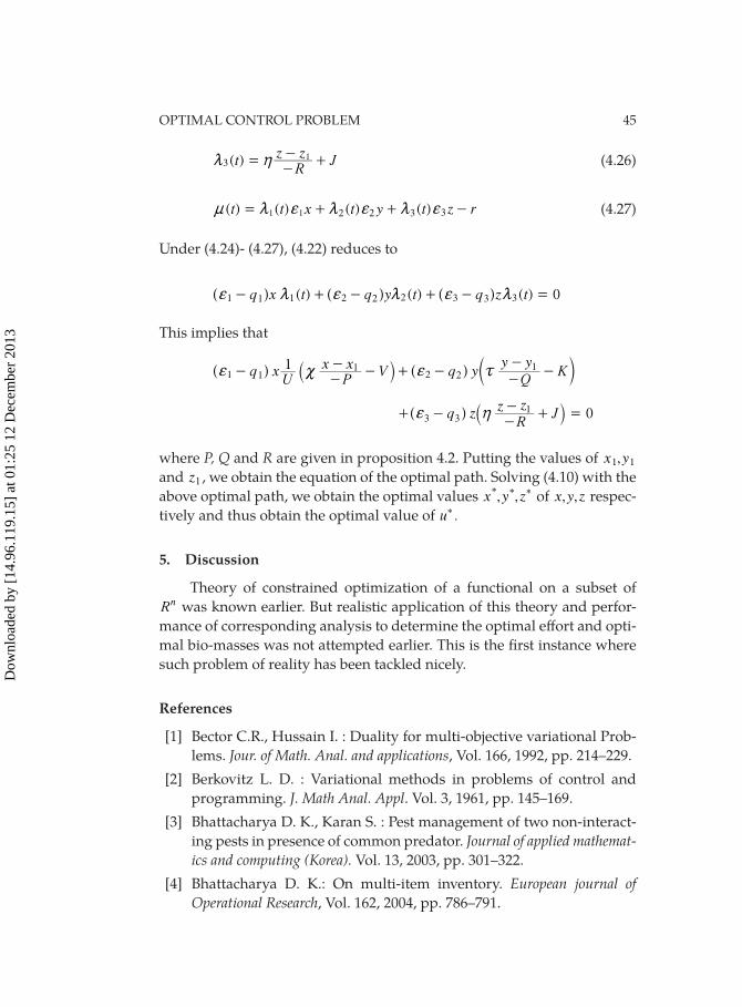
OPTIMAL CONTROL PROBLEM 45

( )tR

z zJ3

1m h=--

+ (4.26)

2( ) ( ) ( ) ( )t t x t y t z rn m f m f m f= + + -31 1 2 3 (4.27)

Under (4.24)- (4.27), (4.22) reduces to

2( ) ( )q x t q y t q zf m f m f- + - + -21 1 2 3 31 3 ( ) 0tm =] ] ]g g g

This implies that

1 12q x

U Px x

V q yQ

y yK1f | f x-

--

- + ---

-1 21] ` ] cg j g m

13

zq z

Rz

Jf h+ ---

+3 0=] `g j

where P, Q and R are given in proposition 4.2. Putting the values of ,x y1 1

and z1 , we obtain the equation of the optimal path. Solving (4.10) with the

above optimal path, we obtain the optimal values , ,x y z* * * of , ,x y z respec-

tively and thus obtain the optimal value of * .u

5. Discussion

Theory of constrained optimization of a functional on a subset of

Rn was known earlier. But realistic application of this theory and perfor-

mance of corresponding analysis to determine the optimal eff ort and opti-

mal bio-masses was not attempted earlier. This is the fi rst instance where

such problem of reality has been tackled nicely.

References

[1] Bector C.R., Hussain I. : Duality for multi-objective variational Prob-

lems. Jour. of Math. Anal. and applications, Vol. 166, 1992, pp. 214–229.

[2] Berkovitz L. D. : Variational methods in problems of control and

programming. J. Math Anal. Appl. Vol. 3, 1961, pp. 145–169.

[3] Bhattacharya D. K., Karan S. : Pest management of two non-interact-

ing pests in presence of common predator. Journal of applied mathemat-ics and computing (Korea). Vol. 13, 2003, pp. 301–322.

[4] Bhattacharya D. K.: On multi-item inventory. European journal of Operational Research, Vol. 162, 2004, pp. 786–791.

Dow

nloa

ded

by [

14.9

6.11

9.15

] at

01:

25 1

2 D

ecem

ber

2013

46 A. GUPTA AND D. K. BHATTACHARYA

[5] Bhattacharya D. K., Bhattacharyya S.: A new approach to pest

management problem. Journal of Biological System, Vol. 13(2), 2005,

pp. 117–130.

[6] Brickell F., Clark R. S. : Diff erentiable Manifold, An introduction. University

of Southampton, Van Nostrand Reinhold Company-London, 1970.

[7] Clark Colin W. : MATHEMATICAL BIOECONOMICS- The Opti-mal Management of Renewable Resources, John Wiley and Sons, Inc.,

New York, 1990.

[8] Elizer Kreindler : Reciprocal optimal control problems. Journal of Mathematical Analysis and Applications, pp. 14, 1966, pp. 141–152.

[9] Gupta A., Bhattacharya D. K. : Generalization of Replicator Dynamics from a 3-simplex to a 2-sphere with boundary. Revista D. La Academia,

Vol. XVIII(1-2), 2006.

[10] Gupta A., Bhattacharya D.K. : Permanence Criteria of Replicator Dynam-ics on a 2-sphere with boundary through Vector Optimization Technique.

Revista D.La Academia, Vol. XIX(1–2), 2007.

[11] Hofbauer J., A general cooperation theorem for hypercycles, Monatsh. Math. Vol. 91, 1988, pp. 233–240.

[12] Pontryagin’s L. S., Bolytyanski V. S., Gamkrelidze R. V., Isch-

enko E. F. : The mathematical theory of optimal process. Wiley Interscience,

New York, 1962.

[13] Schuster P., Sigmud K. and Wolff R., Mass action kinetics of selfrepli-

cation in fl ow reactors, J. Math Anal. Appl. Vol. 78, 1980, pp. 88–112.

[14] Schuster P., Sigmud K., Hofbauer J., Wolff R, Selfregulation of behav-

iour in animal societies., Biol. Cybern, Vol. 40, 1981, pp. 1-25.

[15] Valentine F. A. : The problem of Lagrange with diff erential in-

equalities as added side condition, Contributions to the calculus of

variations. University Chicago press, Chicago, 1937, pp. 407–488.

Received May, 2012

Dow

nloa

ded

by [

14.9

6.11

9.15

] at

01:

25 1

2 D

ecem

ber

2013