Feature-Aware Uniform Tessellations on Video Manifold for ...
13
ACCEPTED BY IEEE T-PAMI 1 Feature-Aware Uniform Tessellations on Video Manifold for Content-Sensitive Supervoxels Ran Yi, Zipeng Ye, Wang Zhao, Minjing Yu, Yu-Kun Lai, Yong-Jin Liu, Senior Member, IEEE Abstract—Over-segmenting a video into supervoxels has strong potential to reduce the complexity of downstream computer vision applications. Content-sensitive supervoxels (CSSs) are typically smaller in content-dense regions (i.e., with high variation of appearance and/or motion) and larger in content-sparse regions. In this paper, we propose to compute feature-aware CSSs (FCSSs) that are regularly shaped 3D primitive volumes well aligned with local object/region/motion boundaries in video. To compute FCSSs, we map a video to a 3-dimensional manifold embedded in a combined color and spatiotemporal space, in which the volume elements of video manifold give a good measure of the video content density. Then any uniform tessellation on video manifold can induce CSS in the video. Our idea is that among all possible uniform tessellations on the video manifold, FCSS finds one whose cell boundaries well align with local video boundaries. To achieve this goal, we propose a novel restricted centroidal Voronoi tessellation method that simultaneously minimizes the tessellation energy (leading to uniform cells in the tessellation) and maximizes the average boundary distance (leading to good local feature alignment). Theoretically our method has an optimal competitive ratio O(1), and its time and space complexities are O(NK) and O(N + K) for computing K supervoxels in an N -voxel video. We also present a simple extension of FCSS to streaming FCSS for processing long videos that cannot be loaded into main memory at once. We evaluate FCSS, streaming FCSS and ten representative supervoxel methods on four video datasets and two novel video applications. The results show that our method simultaneously achieves state-of-the-art performance with respect to various evaluation criteria. Index Terms—Supervoxels, video over-segmentation, video manifold, low-level video features, centroidal Voronoi tessellation. ✦ 1 I NTRODUCTION S UPERVOXELS are perceptually meaningful atomic re- gions obtained by grouping similar voxels (i.e., ex- hibiting coherence in both appearance and motion) in the spatiotemporal domain. As a special over-segmentation of videos, supervoxels well preserve the structural content while still providing sufficient levels of detail. Therefore, supervoxels can greatly reduce the computational complex- ity and have been widely used as a preprocessing step in many computer vision applications, such as video seg- mentation [13], [19], [45], propagation of foreground object segmentation [14], spatiotemporal object detection [27], spa- tiotemporal closure in videos [17], action segmentation and recognition [15], [25], and many others. Many methods have been proposed for computing su- pervoxels, including energy minimization by graph cut [38], non-parametric feature-space analysis [28], graph- based merging [9], [13], [42], contour-evolving optimization [17], [21], [31], optimization of normalized cuts [33], [7], generative probabilistic framework [5] and hybrid cluster- ing [30], [43], etc. These methods can be classified according • R. Yi, Z, Ye, W. Zhao and Y.-J. Liu are with BNRist, MOE-Key Laboratory of Pervasive Computing, the Department of Computer Science and Tech- nology, Tsinghua University, Beijing, China. R. Yi and Z. Ye are joint first authors. E-mail: {yr16@mails., yezp17@mails., zhao-w19@mails., liuyongjin@}tsinghua.edu.cn • M. Yu is with College of Intelligence and Computing, Tianjin University, Tianjin, China. E-mail: [email protected] • Y.-K. Lai is with School of Computer Science and Informatics, Cardiff University, UK. E-mail: [email protected] • M. Yu and Y.-J. Liu are corresponding authors. This work was supported by the Natural Science Foundation of China (61725204, 61521002). to different representation formats: (1) temporal superpixels [5], [4], [17], [21], [30], [31], [39]: supervoxels are represented in each frame and their labels are temporally consistent in adjacent frames, and (2) supervoxels [7], [9], [13], [28], [33], [38], [42], [43]: they are 3D primitive volumes whose union forms the video volume. Note that these two rep- resentations can be transferred to each other. For example, temporal superpixels can be stacked up frame-by-frame to reconstruct supervoxels. However, individual supevoxels obtained in this way may have disconnected components or have a complex topology type (i.e., having a non-zero genus). On the other hand, a supervoxel can be sliced by related frames to decompose it into temporal superpixels, however, a superpixel sliced in a frame may also consist of disjoint components or have a complex topology type. Depending on the size of video data, supervoxel meth- ods can also be classified into off-line and streaming methods. Off-line methods require the video to be short enough such that all video data can be loaded into the memory. On the other hand, streaming methods do not have such a limitation on the video length, i.e., video data is accessed sequentially in blocks and each time only a block is needed to feed into the memory. In a recent survey [41], seven representative supervoxel methods are selected, including five off-line [9], [10], [28], [7], [13] and two streaming [42], [5] methods, to represent the state of the art. To measure the quality of supervoxels, the following principles have been considered in previous work [13], [22], [38], [41], [24], [44]: (1) Feature preservation: supervoxel boundaries align well with object/region/motion bound- aries in a video; (2) Spatiotemporal uniformity: in non-feature regions, supervoxels are uniform and regular in the spa- tiotemporal domain; (3) Performance: computing supervox-
-
Upload
khangminh22 -
Category
Documents
-
view
1 -
download
0
Transcript of Feature-Aware Uniform Tessellations on Video Manifold for ...

ACCEPTED BY IEEE T-PAMI 1
Feature-Aware Uniform Tessellations on VideoManifold for Content-Sensitive Supervoxels
Ran Yi, Zipeng Ye, Wang Zhao, Minjing Yu, Yu-Kun Lai, Yong-Jin Liu, Senior Member, IEEE
Abstract—Over-segmenting a video into supervoxels has strong potential to reduce the complexity of downstream computer visionapplications. Content-sensitive supervoxels (CSSs) are typically smaller in content-dense regions (i.e., with high variation ofappearance and/or motion) and larger in content-sparse regions. In this paper, we propose to compute feature-aware CSSs (FCSSs)that are regularly shaped 3D primitive volumes well aligned with local object/region/motion boundaries in video. To compute FCSSs, wemap a video to a 3-dimensional manifold embedded in a combined color and spatiotemporal space, in which the volume elements ofvideo manifold give a good measure of the video content density. Then any uniform tessellation on video manifold can induce CSS inthe video. Our idea is that among all possible uniform tessellations on the video manifold, FCSS finds one whose cell boundaries wellalign with local video boundaries. To achieve this goal, we propose a novel restricted centroidal Voronoi tessellation method thatsimultaneously minimizes the tessellation energy (leading to uniform cells in the tessellation) and maximizes the average boundarydistance (leading to good local feature alignment). Theoretically our method has an optimal competitive ratio O(1), and its time andspace complexities are O(NK) and O(N + K) for computing K supervoxels in an N -voxel video. We also present a simple extensionof FCSS to streaming FCSS for processing long videos that cannot be loaded into main memory at once. We evaluate FCSS,streaming FCSS and ten representative supervoxel methods on four video datasets and two novel video applications. The results showthat our method simultaneously achieves state-of-the-art performance with respect to various evaluation criteria.
Index Terms—Supervoxels, video over-segmentation, video manifold, low-level video features, centroidal Voronoi tessellation.
F
1 INTRODUCTION
SUPERVOXELS are perceptually meaningful atomic re-gions obtained by grouping similar voxels (i.e., ex-
hibiting coherence in both appearance and motion) in thespatiotemporal domain. As a special over-segmentation ofvideos, supervoxels well preserve the structural contentwhile still providing sufficient levels of detail. Therefore,supervoxels can greatly reduce the computational complex-ity and have been widely used as a preprocessing stepin many computer vision applications, such as video seg-mentation [13], [19], [45], propagation of foreground objectsegmentation [14], spatiotemporal object detection [27], spa-tiotemporal closure in videos [17], action segmentation andrecognition [15], [25], and many others.
Many methods have been proposed for computing su-pervoxels, including energy minimization by graph cut[38], non-parametric feature-space analysis [28], graph-based merging [9], [13], [42], contour-evolving optimization[17], [21], [31], optimization of normalized cuts [33], [7],generative probabilistic framework [5] and hybrid cluster-ing [30], [43], etc. These methods can be classified according
• R. Yi, Z, Ye, W. Zhao and Y.-J. Liu are with BNRist, MOE-Key Laboratoryof Pervasive Computing, the Department of Computer Science and Tech-nology, Tsinghua University, Beijing, China. R. Yi and Z. Ye are jointfirst authors. E-mail: yr16@mails., yezp17@mails., zhao-w19@mails.,[email protected]
• M. Yu is with College of Intelligence and Computing, Tianjin University,Tianjin, China. E-mail: [email protected]
• Y.-K. Lai is with School of Computer Science and Informatics, CardiffUniversity, UK. E-mail: [email protected]
• M. Yu and Y.-J. Liu are corresponding authors.
This work was supported by the Natural Science Foundation of China(61725204, 61521002).
to different representation formats: (1) temporal superpixels[5], [4], [17], [21], [30], [31], [39]: supervoxels are representedin each frame and their labels are temporally consistentin adjacent frames, and (2) supervoxels [7], [9], [13], [28],[33], [38], [42], [43]: they are 3D primitive volumes whoseunion forms the video volume. Note that these two rep-resentations can be transferred to each other. For example,temporal superpixels can be stacked up frame-by-frame toreconstruct supervoxels. However, individual supevoxelsobtained in this way may have disconnected componentsor have a complex topology type (i.e., having a non-zerogenus). On the other hand, a supervoxel can be sliced byrelated frames to decompose it into temporal superpixels,however, a superpixel sliced in a frame may also consist ofdisjoint components or have a complex topology type.
Depending on the size of video data, supervoxel meth-ods can also be classified into off-line and streaming methods.Off-line methods require the video to be short enough suchthat all video data can be loaded into the memory. Onthe other hand, streaming methods do not have such alimitation on the video length, i.e., video data is accessedsequentially in blocks and each time only a block is neededto feed into the memory. In a recent survey [41], sevenrepresentative supervoxel methods are selected, includingfive off-line [9], [10], [28], [7], [13] and two streaming [42],[5] methods, to represent the state of the art.
To measure the quality of supervoxels, the followingprinciples have been considered in previous work [13],[22], [38], [41], [24], [44]: (1) Feature preservation: supervoxelboundaries align well with object/region/motion bound-aries in a video; (2) Spatiotemporal uniformity: in non-featureregions, supervoxels are uniform and regular in the spa-tiotemporal domain; (3) Performance: computing supervox-

ACCEPTED BY IEEE T-PAMI 2Frame21
Frame41
Frame61
Original frame GB GBH SWA MeanShift TSP TS-PPM CSS FCSS
Fig. 1. Superpixels (induced by clipping supervoxels on frames #21, #41 and #61) obtained by GB [9], GBH [13], SWA [32], [33], [7], MeanShift [28],TSP [5], TS-PPM [16], CSS [43] and our FCSS. All methods generate approximately 1,500 supervoxels. TSP, TS-PPM, CSS and FCSS produceregular supervoxels (and accordingly regular clipped superpixels), while other methods produce highly irregular supervoxels. As shown in Section6, these four methods are insensitive to supervoxel relabeling and achieve a good balance among commonly used quality metrics pertaining tosupervoxels, including UE3D, SA3D, BRD and EV, while FCSS runs 5× to 10× faster than TSP, and the peak memory required by FCSS is 22×smaller than TSP and 7× to 15× smaller than TS-PPM. Both FCSS and CSS generate more supervoxels in content-rich areas (e.g., bushes onthe lake shore) and fewer supervoxels in content-sparse areas (e.g., lake surface), while FCSS better captures low-level video features (e.g., localobject/region/motion boundaries) than CSS, leading to better performance in two video applications (Section 7). See Appendix for more visualcomparison and accompanying demo video for more dynamic details.
els is time-and-space efficient and scales well with largevideo data; (4) Easy to use: users simply specify the desirednumber of supervoxels and should not be bothered to tuneother parameters; (5) Parsimony: the above principles areachieved with as few supervoxels as possible.
So far, none of existing methods satisfy all above prin-ciples. In our previous work [43], we propose a content-sensitive approach to address the parsimony principle. Thisapproach is motivated by an important observation: thescene layouts and motions of different objects in a videousually exhibit large diversity, and thus the density of videocontent often varies significantly in different parts of thevideo. Generating spatiotemporally uniform supervoxelsindiscriminately in the whole video often leads to under-segmentation in content-dense regions (i.e., with high varia-tion of appearance and/or motion), and over-segmentationin content-sparse regions (i.e., with homogeneous appear-ance and motion). Therefore, computing supervoxels adap-tively with respect to the density of video content canachieve a good balance among different principles.
To compute content-sensitive supervoxels (CSSs), Yi etal. [43] map a video Υ to 3-manifold M embedded in afeature space R6. The map Φ is designed in such a waythat the volumetric elements inM give a good measure ofcontent density in Υ, and thus, a uniform tessellation T onM efficiently induces CSSs (i.e., Φ−1(T )) in Υ. In this paper,we improve upon our previous work [43] and proposefeature-aware CSS (FCSS). Our key idea is that among allpossible uniform tessellations on M, we find one whosecell boundaries well align with local object/region/motionboundaries in video. To achieve this goal, we improve the re-stricted centroidal Voronoi tessellation (RCVT) method [23],[43] and make the following contributions.
• To measure the degree of alignment between RCVT’scell boundaries and local video features, we proposean average boundary distance measure dbdry and useit to control the positions of generating points inRCVT.
• We formulate FCSSs by simultaneously minimizingthe RCVT energy (leading to uniform cells in RCVT)and maximizing dbdry (leading to good local feature
alignment).• To quickly compute FCSSs, we propose a splitting-
merging scheme that can be efficiently incorporatedinto the well known K-means++ algorithm [2], [40].
Our method has a theoretical constant-factor bi-criteria ap-proximation guarantee, and in practice our method canobtain good supervoxels in very few iterations. By applyingthe streaming version of K-means++ (a.k.a. K-means# [1]),our method can be easily extended to process long videosthat cannot be loaded into main memory at once. We thor-oughly evaluate FCSS, streaming FCSS and ten representa-tive supervoxel methods on four video datasets. A visualcomparison is shown in Figure 1. The results show that ourmethod achieves a good balance among over-segmentationaccuracies (UE3D, SA3D, BRD and EV in Section 6), com-pactness, and time and space efficiency. As a case study,we also evaluate these methods on two novel applications(foreground propagation in video [14] and optimal videoclosure [17]) and the results show that FCSS achieves thebest propagation and spatiotemporal closure performance.
2 PRELIMINARIES
Our method improves the CSS work [43] that uses RCVTto compute a uniform tessellation of a 3-manifoldM⊂ R6.Theoretically our method is a bi-criteria approximation to theK-means problem [2], [1], [40]. We briefly introduce thembefore presenting our method.
2.1 Video manifoldM and CSSSimply treating the time dimension in a video equivalentlyas spatial dimensions results in a regular 3D lattice represen-tation of voxels in R3, which is not proper due to possiblynon-negligible motions and occlusions/disocclusions. Toovercome this drawback, some methods (e.g., [13], [5]) useoptical flow to re-establish a connection graph of neighbor-ing voxels between adjacent frames. However, even state-of-the-art optical flow estimation methods [36] are stillimperfect and may introduce extra errors into supervoxelcomputation. Recently, Reso et al. [31] propose a novelformulation specifically designed for handling occlusions.

ACCEPTED BY IEEE T-PAMI 3
a2 a3a1
U R3
F(v)
F(a4)
F(a2)F(a3)
(x-1,y-1,t-1)
(x+1,y+1,t+1)
va4
a5
a7
a8F(a5)
F(a6) F(a7)
F(a8)
M = F(U) R6
Mapping F
x
yt
F(a1)
a6
v = (x,y,t)
Fig. 2. Left: regular 3D lattices of voxels in R3. Middle and right: themap Φ : Υ → M ⊂ R6 stretches the unit cube v (red box) centeredat the voxel v(x, y, t) ∈ Υ into a 3-manifoldM. Each corner ai of v ,i = 1, 2, · · · , 8, is the center of its eight neighboring voxels.
On the contrary, without any special treatment for occlu-sions, the video manifold M proposed in [43] providesan elegant continuous search space that circumvents theaforementioned drawback.
In [43], M is constructed as a 3-manifold embeddedin a combined color and spatiotemporal space R6, whichstretches a video Υ by a map Φ : Υ→M⊂ R6 (Figure 2):
Φ(v) = (λ1x, λ1y, λ2t, λ3l(v), λ3a(v), λ3b(v)) , (1)
where a voxel v ∈ Υ is represented by (x, y, t), (x, y) is thepixel location and t the frame index. (l(v), a(v), b(v)) is thecolor at the voxel v in the CIELAB color space. λ1 = λ2 =0.435 and λ3 = 1 are global stretching factors.
The volume of a region Φ(Ω) ⊂ M depends on boththe volume of Ω ⊂ Υ and the color variation in Ω. Thehigher variation of colors in Ω (indicating higher variation ofappearance and/or motion), the larger the volume of Φ(Ω).Therefore, the volume form onM gives a good measure ofcontent density in Υ and the inverse mapping Φ−1 of anyuniform tessellation onM generates CSSs in Υ.
To measure the volume in M, ∀v ∈ Υ, the volumeV (Φ(v)) of Φ(v) ⊂ M is quickly evaluated onlyonce [43], where v is the unit cube centered at the voxel v(Figure 2 middle). Then the volume of Φ(Ω) ⊂M is simplythe sum Σvj∈ΩV (Φ(vj )).
2.2 Restricted Voronoi tessellation and RCVTRCVT has been used to build uniform tessellations on man-ifolds [23], [43]. Denote by SK = siKi=1 a set of generatingpoints and M a 3-manifold in R6. The Euclidean Voronoicell of a generator si in R6, denoted by CR6 , is
CR6(si) , x ∈ R6 : ‖x− si‖2 ≤ ‖x− sj‖2,∀j 6= i, sj ∈ SK.
(2)
The restricted Voronoi cell CM is defined to be the intersec-tion of CR6 andM
CM(si) ,M∩ CR6(si), (3)
and its mass centroid is
mi ,
∫x∈CM(si)
xdx∫x∈CM(si)
dx. (4)
The restricted Voronoi tessellation RV T (SK ,M) is the col-lection of restricted Voronoi cells
RV T (SK ,M) , CM(si) 6= ∅,∀si ∈ SK, (5)
which is a finite closed covering ofM. An RV T (SK ,M) isan RCVT if and only if each generator si ∈ SK is the masscentroid of CM(si).
Theorem 1. [23], [43] Let M be a 3-manifold embedded in R6
and K ∈ Z+ be a positive integer. For an arbitrary set SK ofpoints siKi=1 in R6 and an arbitrary tessellation CiKi=1 onM,
⋃Ki=1 Ci =M, Ci
⋂Cj = ∅, ∀i 6= j, define the tessellation
energy functional as follows:
E((si, Ci)Ki=1) =K∑i=1
∫x∈Ci
‖x− si‖22dx. (6)
Then the necessary condition for E to be minimized is that(si, Ci)Ki=1 is an RCVT ofM.
Theorem 1 indicates that RCVT is a uniform tessellationonM, which minimizes the energy E .
2.3 Bi-criteria approximation algorithms
The discretized counterpart of RCVT is the solution tothe K-means problem on the manifold domain M. Givena fixed K , denote by SoptK = sopti Ki=1 and Copti Ki=1
the (unknown) optimal generator set and tessellation onM, respectively, which minimize the energy E . Let SKand CiKi=1 be the generator set and tessellation outputfrom an algorithm A. An algorithm A is said to be b-approximation if for all instances of the problem, it producesa solution si, CiKi=1 satisfying E((si,Ci)Ki=1)
E((sopti ,Copti )Ki=1)
≤ b.An algorithm is called (a, b)-approximation, if it outputs(si, Ci)aKi=1 with aK generators and tessellation cells, suchthat E((si,Ci)aK
i=1)
E((sopti ,Copti )Ki=1)
≤ b, where a > 1 and b > 1.
3 OVERVIEW OF FCSS
The classic Lloyd method is used in [23], [43] to computeRCVT on manifoldM, which iteratively moves each gener-ator si to the corresponding mass centroid of CM(si) andupdates the RVT. Note that the Lloyd method converges toa local minimum. Among all possible local minimums (eachcorresponding to a uniform tessellation onM), we proposeFCSS which aims at finding one whose cell boundaries wellalign with local video boundaries. To achieve this goal,our FCSS method is built upon an important observation:when the set of generating points are far away from localobject/region/motion boundaries inM, the cell boundariesof their RCVT will well align with these local video bound-aries. See Figure 3 for an illustration.
In a video Υ, local boundaries most likely appear inregions with high variation of appearance. Therefore, wecan characterize these local regions in M by the volumeV (Φ(v)): the larger the volume V (Φ(v)), the higher theprobability that the voxel v lies on a local boundary. SinceV (Φ(v)) ≥ 1 and it can be extremely large at sharpboundaries, we use the following nonlinear normalization:
pbdry(v) =2
πarctan(V (Φ(v))) (7)
to characterize the possibility of a voxel v being on the localboundary. Then our objective can be casted as finding a setof generating points siKi=1, in which each si is around themapped position Φ(v′) of a voxel v′ with low boundary

ACCEPTED BY IEEE T-PAMI 4
A local minimum
of tessellation energy = 4.4E+7
Average boundary distance = 2.1E+7
A local minimum
of tessellation energy = 4.3E+7
Average boundary distance = 2.2E+7
I
t
Video manifold
CSS FCSS
-1 -1
Fig. 3. Comparison of FCSS and CSS generation on a synthetic, de-generate gray video Υ, for easy illustration. In Υ, each image frameat time t is a degenerate 1D gray line image It. Supervoxels aregenerated by a tessellation in Υ. Left: Υ is mapped to a video manifoldM = Φ(I, t) ⊂ R3, whose area elements give a good measureof content density in Υ. Middle and right: two local minimums of thetessellation energy specified in Eq.(6). The generating points are shownin dots on M and their inverse images by Φ−1 are shown in redcrosses + in Υ. In this toy example, the local boundaries in Υ can becharacterized by the zero crossing of the second derivative of Υ(I, t)(shown in red circles in left). Note that the tessellations in middle andright are generated without this information. The generating points inFCSS are farther away from local boundaries (indicating by a largeraverage boundary distance proposed in Eq.(8)), and the cell boundariesof the corresponding tessellation better capture these local boundariesthan that of CSS.
possibility pbdry(v′). We formulate this objective by propos-ing an average boundary distance (ABD) for a tessellationsi, CiKi=1:
dbdry((si, Ci)Ki=1
)=
K∑i=1
∫x∈Ci
pbdry(x)‖x− si‖22dx, (8)
where pbdry(x) = pbdry(Φ−1(x)). The larger the distancedbdry is, the farther siKi=1 are from the local boundaries.Two examples are shown in Figure 3: the average boundarydistances of the middle and right tessellations are 2.1× 10⁷
and 2.2× 10⁷, respectively.In the next section, we implement FCSS using a variant
of the Lloyd method that finds a uniform tessellation byminimizing the tessellation energy defined in Eq.(6) in sucha way that the optimal generating points are determinedby minimizing the following ABD-weighted tessellationenergy:
Eα((si, Ci)Ki=1
)=
E((si, Ci)Ki=1
)− αdbdry
((si, Ci)Ki=1
)=∑K
i=1
∫x∈Ci
(1− αpbdry(x))‖x− si‖22dx,(9)
where α > 0 is a weight to balance the two terms E anddbdry . In all our experiments, we set α = 0.8.
4 IMPLEMENTATION OF FCSSTo obtain a feature-aware uniform tessellation (si, Ci)Ki=1
inM, our FCSS method consists of the following two steps:
• Initialization (Section 4.1). We apply a variant of theK-means++ algorithm [2], [1], [40] to determine the
Algorithm 1 InitializationInput: A video Υ of N voxels and the desired number of
supervoxels K .Output: The initial positions of K generating points SK =siKi=1.
1: Compute V (Φ(v)) for each voxel v ∈ Υ.2: Choose a point v1 from all voxels v ∈ Υ with probability
proportional to V (Φ(v)).3: Set s1 = Φ(v1), S1 = s1 and j = 1.4: while j < K do5: Choose a point vj+1 from all voxels v ∈ Υ with
probability proportional to the cost cSj (v) (Eq.(11)).6: Set sj+1 = Φ(vj+1), Sj+1 = Sj∪sj+1 and j = j+1.7: end while
initial positions of generating points SK = siKi=1,which ensures an (O(1), O(1))-approximation.
• Feature-aware Lloyd refinement (Section 4.2). Ob-serving that the classic Lloyd method convergesonly to a local minimum and without feature-awarecontrol on the positions of generating points, weoptimize the tessellation and the positions of gen-erating points separately by minimizing two energyforms (i.e., Eqs. (6) and (9)), leading to a local min-imum of the content-sensitive uniform tessellationon the manifold M that also optimizes the averageboundary distance dbdry to improve feature align-ment of cell boundaries. We further propose an ef-ficient splitting-merging scheme that helps move thesolution out of local minimums, while preserving theapproximation ratio.
The FCSS method is easy to implement and can obtainhigh-quality supervoxels in very few iterations. Theoreti-cally FCSS is (O(1), O(1))-approximation (Section 4.3). Wealso present a simple extension of FCSS to streaming FCSSfor processing long videos (Section 5).
4.1 InitializationWe apply a variant of K-means++ algorithm to obtaina provable high-quality initialization of generating pointsSK = siKi=1. The pseudo-code is summarized in Algo-rithm 1. In each step, a point in M is picked up withprobability proportional to its current cost (defined as itssquared distance to the nearest generator picked so far),and added as a new generator. To compute the requiredprobability in the manifold domain M, we consider thepositions of mapped voxels Φ(v) ∈ M, ∀v ∈ Υ. Withrespect to an existing generator Φ(vi), the cost of a mappedvoxel Φ(vj) ∈M, j 6= i, is
cvi(vj) =∫x∈Φ(vj
) ‖x− Φ(vi)‖22dx≈ V (Φ(vj )) · ‖Φ(vj)− Φ(vi)‖22
(10)
Then the cost of picking Φ(vj) with respect to an existinggenerator set S is
cS(vj) = minvi∈S
cvi(vj) (11)
Algorithm 1 runs in O(NK) time. A simple adaption of theproofs in [2], [40] shows the following results.
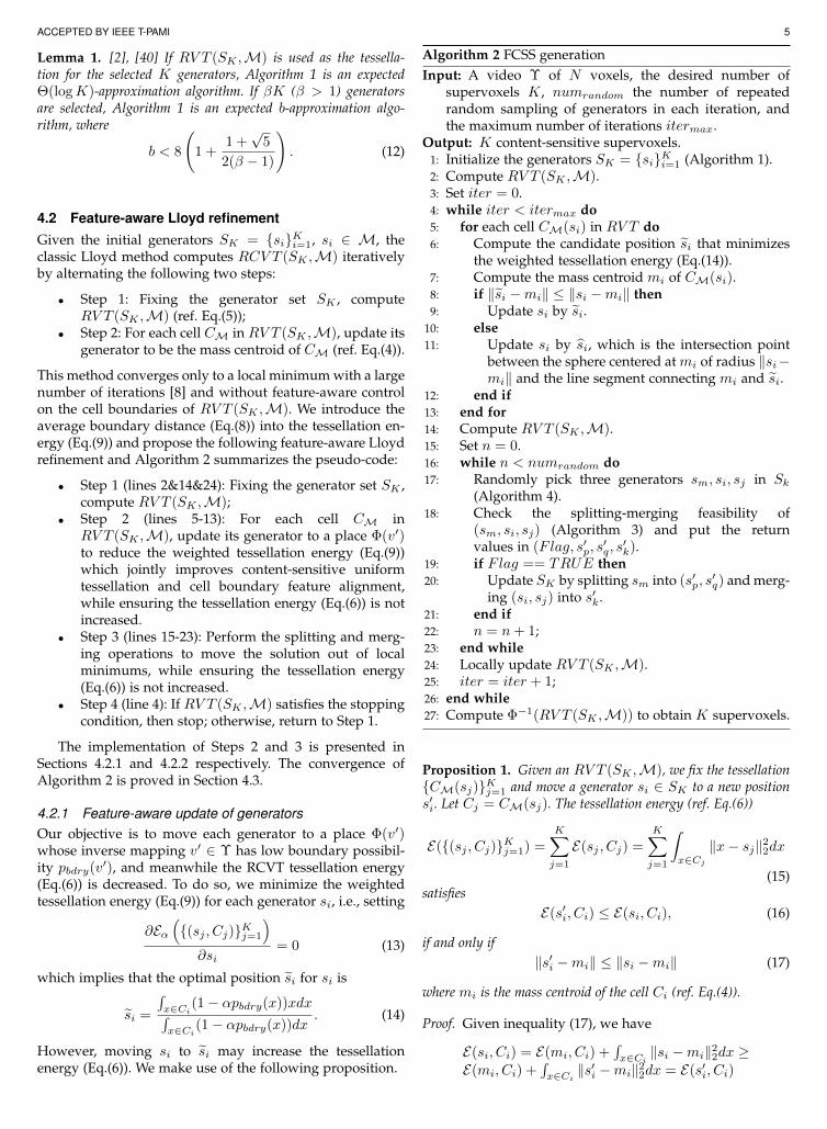
ACCEPTED BY IEEE T-PAMI 5
Lemma 1. [2], [40] If RV T (SK ,M) is used as the tessella-tion for the selected K generators, Algorithm 1 is an expectedΘ(logK)-approximation algorithm. If βK (β > 1) generatorsare selected, Algorithm 1 is an expected b-approximation algo-rithm, where
b < 8
(1 +
1 +√
5
2(β − 1)
). (12)
4.2 Feature-aware Lloyd refinementGiven the initial generators SK = siKi=1, si ∈ M, theclassic Lloyd method computes RCV T (SK ,M) iterativelyby alternating the following two steps:
• Step 1: Fixing the generator set SK , computeRV T (SK ,M) (ref. Eq.(5));
• Step 2: For each cell CM in RV T (SK ,M), update itsgenerator to be the mass centroid of CM (ref. Eq.(4)).
This method converges only to a local minimum with a largenumber of iterations [8] and without feature-aware controlon the cell boundaries of RV T (SK ,M). We introduce theaverage boundary distance (Eq.(8)) into the tessellation en-ergy (Eq.(9)) and propose the following feature-aware Lloydrefinement and Algorithm 2 summarizes the pseudo-code:
• Step 1 (lines 2&14&24): Fixing the generator set SK ,compute RV T (SK ,M);
• Step 2 (lines 5-13): For each cell CM inRV T (SK ,M), update its generator to a place Φ(v′)to reduce the weighted tessellation energy (Eq.(9))which jointly improves content-sensitive uniformtessellation and cell boundary feature alignment,while ensuring the tessellation energy (Eq.(6)) is notincreased.
• Step 3 (lines 15-23): Perform the splitting and merg-ing operations to move the solution out of localminimums, while ensuring the tessellation energy(Eq.(6)) is not increased.
• Step 4 (line 4): If RV T (SK ,M) satisfies the stoppingcondition, then stop; otherwise, return to Step 1.
The implementation of Steps 2 and 3 is presented inSections 4.2.1 and 4.2.2 respectively. The convergence ofAlgorithm 2 is proved in Section 4.3.
4.2.1 Feature-aware update of generatorsOur objective is to move each generator to a place Φ(v′)whose inverse mapping v′ ∈ Υ has low boundary possibil-ity pbdry(v′), and meanwhile the RCVT tessellation energy(Eq.(6)) is decreased. To do so, we minimize the weightedtessellation energy (Eq.(9)) for each generator si, i.e., setting
∂Eα((sj , Cj)Kj=1
)∂si
= 0 (13)
which implies that the optimal position si for si is
si =
∫x∈Ci
(1− αpbdry(x))xdx∫x∈Ci
(1− αpbdry(x))dx. (14)
However, moving si to si may increase the tessellationenergy (Eq.(6)). We make use of the following proposition.
Algorithm 2 FCSS generationInput: A video Υ of N voxels, the desired number of
supervoxels K, numrandom the number of repeatedrandom sampling of generators in each iteration, andthe maximum number of iterations itermax.
Output: K content-sensitive supervoxels.1: Initialize the generators SK = siKi=1 (Algorithm 1).2: Compute RV T (SK ,M).3: Set iter = 0.4: while iter < itermax do5: for each cell CM(si) in RV T do6: Compute the candidate position si that minimizes
the weighted tessellation energy (Eq.(14)).7: Compute the mass centroid mi of CM(si).8: if ‖si −mi‖ ≤ ‖si −mi‖ then9: Update si by si.
10: else11: Update si by si, which is the intersection point
between the sphere centered at mi of radius ‖si−mi‖ and the line segment connecting mi and si.
12: end if13: end for14: Compute RV T (SK ,M).15: Set n = 0.16: while n < numrandom do17: Randomly pick three generators sm, si, sj in Sk
(Algorithm 4).18: Check the splitting-merging feasibility of
(sm, si, sj) (Algorithm 3) and put the returnvalues in (Flag, s′p, s
′q, s′k).
19: if Flag == TRUE then20: Update SK by splitting sm into (s′p, s
′q) and merg-
ing (si, sj) into s′k.21: end if22: n = n+ 1;23: end while24: Locally update RV T (SK ,M).25: iter = iter + 1;26: end while27: Compute Φ−1(RV T (SK ,M)) to obtain K supervoxels.
Proposition 1. Given an RV T (SK ,M), we fix the tessellationCM(sj)Kj=1 and move a generator si ∈ SK to a new positions′i. Let Cj = CM(sj). The tessellation energy (ref. Eq.(6))
E((sj , Cj)Kj=1) =K∑j=1
E(sj , Cj) =K∑j=1
∫x∈Cj
‖x− sj‖22dx
(15)satisfies
E(s′i, Ci) ≤ E(si, Ci), (16)
if and only if‖s′i −mi‖ ≤ ‖si −mi‖ (17)
where mi is the mass centroid of the cell Ci (ref. Eq.(4)).
Proof. Given inequality (17), we have
E(si, Ci) = E(mi, Ci) +∫x∈Ci
‖si −mi‖22dx ≥E(mi, Ci) +
∫x∈Ci
‖s′i −mi‖22dx = E(s′i, Ci)

ACCEPTED BY IEEE T-PAMI 6
Algorithm 3 Check splitting-merging feasibilityInput: Three generators (sm, si, sj) in SK and an
RV T (SK ,M).Output: A Boolean variable Flag indicating the feasibility
and three new generators (s′p, s′q, s′k).
1: Compute the mass centroids s′m, s′i and s′j of CM(sm),CM(si) and CM(sj), respectively.
2: Compute the diameter dm of the cell CM(sm) and thepoints pm1 and pm2 (see Definition 1).
3: Compute two new cellsC ′(pm1) andC ′(pm2), which arethe Voronoi cells of pm1 and pm2 in the domainCM(sm).
4: Compute the mass centroids s′k, s′p and s′q of CM(si) ∪CM(sj), C ′(pm1) and C ′(pm2), respectively.
5: Compute τm,i,j in Eq. (20).6: if ‖s′p − s′m‖2 > τm,i,j and ‖s′q − s′m‖2 > τm,i,j then7: return TRUE and (s′p, s
′q, s′k).
8: else9: return FALSE and (NULL,NULL,NULL).
10: end if
On the other hand, if E(si, Ci) ≥ E(s′i, Ci), then we have∫x∈Ci
‖mi− si‖22dx ≥∫x∈Ci
‖mi− s′i‖22dx, indicating ‖mi−si‖ ≥ ‖mi − s′i‖. That completes the proof.
In Algorithm 2 (lines 8-9), we check the condition inEq.(17) using the optimal position si. If it is satisfied, weupdate si by si. Otherwise, we set si by moving alongthe direction from mi to si (the average boundary distancedbdry is expected to be increased along this direction) andlocating it at the boundary of the sphere centered at mi ofradius ‖si −mi‖ (moving si to this place does not increasethe tessellation energy). In both cases, we try to reduce theweighted tessellation energy, while ensuring the tessellationenergy is not increased.
4.2.2 Splitting and merging operationsIn Algorithm 2 (lines 16-23), we perform splitting and merg-ing operations for jumping out of a small local search areain M while the tessellation energy still does not increase.We find that these splitting and merging operations helpAlgorithm 2 obtain high-quality supervoxels in very fewiterations.
A splitting operation ∧ : sm → (s′p, s′q) splits an RVT cell
CM(sm) into two new cells C(s′p) and C(s′q). Conversely,a merging operation ∨ : (si, sj) → s′k merges two RVTcells CM(si) and CM(sj) into a new cell C(s′k). Splittingreduces the tessellation energy and merging increases it. Thenumber of generators does not change by applying a pair ofsplitting and merging operations (∧,∨) : (sm, (si, sj)) →((s′p, s
′q), s
′k). Our goal is to design a pair (∧,∨) that does
not increase the tessellation energy. We make use of thefollowing definition and proposition.
Definition 1. The diameter di of a cell CM(si), si ∈ SK , is themaximum Euclidean distance between pairs of points in the cell,i.e.,
di = max∀x,y∈CM(si)
‖x− y‖2 (18)
Denote by pi1 and pi2 the two points inCM(si) satisfying ‖pi1−pi2‖ = di.
pm1pm2
dm
s'm s'q
s'pC'1 C'2
Fig. 4. The diameter dm = ‖pm1 − pm2‖2 of an RVT cell CM(sm)(shaded area) is the maximum Euclidean distance between pairs ofpoints in this cell. The splitting operation ∧ : sm → (s′p, s
′q) splits an
RVT cell CM(sm) (shaded area) into two arbitrary new cells C′1 (orangeshaded area) and C′2 (green shaded area), satisfying pm1 ∈ C′1 andpm2 ∈ C′2, C′1 ∩ C′2 = ∅ and C′1 ∪ C′2 = CM(sm). The mass centroidsof cells CM(sm), C′1 and C′2 are s′m, s′p, s′q , respectively. Lemma 2proves that s′m lies on the line segment connecting s′p and s′q .
Proposition 2. Let sm, si, sj be three generators in anRV T (SK ,M). Let (mm,mi,mj) and (s′m, s
′i, s′j) be the
masses and mass centroids of the cells CM(sm), CM(si),CM(sj), respectively. Consider a splitting of CM(sm) into twoarbitrary new cells C ′1 and C ′2, which satisfies pm1 ∈ C ′1,pm2 ∈ C ′2, C ′1 ∩ C ′2 = ∅ and C ′1 ∪ C ′2 = CM(sm). Let s′p, s
′q
and s′k be the mass centroids of C ′1, C ′2 and CM(si) ∪ CM(sj),respectively. If
‖s′p − s′m‖2 > τm,i,j and ‖s′q − s′m‖2 > τm,i,j , (19)
whereτm,i,j =
√mimj
mm(mi +mj)‖s′i − s′j‖2 (20)
then the pair of operations (∧,∨) : (sm, (si, sj)) →((s′p, s
′q), s
′k) do not increase the tessellation energy E in Eq.(6).
Proof. See Appendix.
To ensure the pair of operations (∧,∨) do not increasethe tessellation energy E , in Algorithm 2 (lines 16-21), wecheck the splitting-merging feasibility condition (Eq.(19))and Algorithm 3 summarizes the pseudo-code. Note thatcomputing the diameter of an arbitrary region (line 2 of Al-gorithm 3) is time-consuming. In practice, we compute theaxis-aligned bounding box B of CM(sm). B is determinedby two supporting points p1 and p2 in CM(sm) and we usethem as fast approximations to pm1 and pm2.
Lemma 2. Let s′m, s′p and s′q be the mass centroids as specifiedin Proposition 2. Then s′m lies on the line segment connecting s′pand s′q .
Proof. Refer to Figure 4. Let mm, m1 and m2 be the massesof CM(sm), C ′1 and C ′2. Since C ′1 ∩ C ′2 = ∅ and C ′1 ∪ C ′2 =CM(sm), we have
s′m =
∫x∈CM (sm) x dx
mm=
∫x∈C′
1x dx+
∫x∈C′
2x dx
m1+m2=
m1s′p+m2s
′q
m1+m2= m1
m1+m2s′p + m2
m1+m2s′q
(21)
That completes the proof.
Note that for a region Ω ⊂ Υ with a fixed volume, thehigher variation of colors in Ω, the larger the volume ofΦ(Ω) ⊂ M and vice versa. Lemma 2 and Proposition 2imply the following important geometric observation:
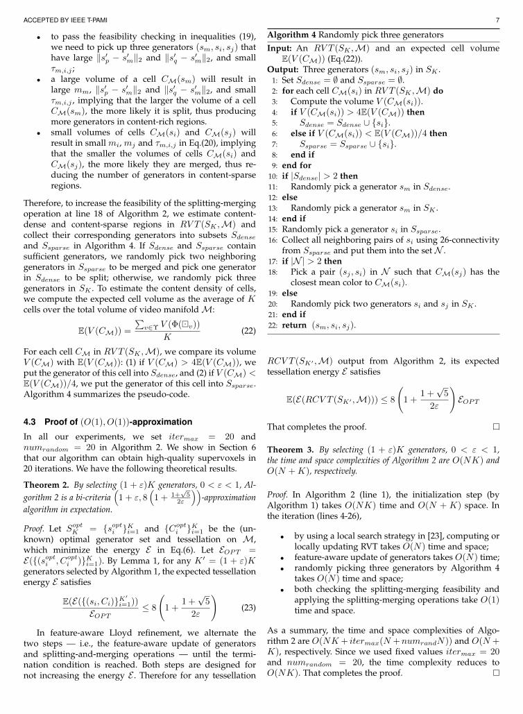
ACCEPTED BY IEEE T-PAMI 7
• to pass the feasibility checking in inequalities (19),we need to pick up three generators (sm, si, sj) thathave large ‖s′p − s′m‖2 and ‖s′q − s′m‖2, and smallτm,i,j ;
• a large volume of a cell CM(sm) will result inlarge mm, ‖s′p − s′m‖2 and ‖s′q − s′m‖2, and smallτm,i,j , implying that the larger the volume of a cellCM(sm), the more likely it is split, thus producingmore generators in content-rich regions.
• small volumes of cells CM(si) and CM(sj) willresult in small mi, mj and τm,i,j in Eq.(20), implyingthat the smaller the volumes of cells CM(si) andCM(sj), the more likely they are merged, thus re-ducing the number of generators in content-sparseregions.
Therefore, to increase the feasibility of the splitting-mergingoperation at line 18 of Algorithm 2, we estimate content-dense and content-sparse regions in RV T (SK ,M) andcollect their corresponding generators into subsets Sdenseand Ssparse in Algorithm 4. If Sdense and Ssparse containsufficient generators, we randomly pick two neighboringgenerators in Ssparse to be merged and pick one generatorin Sdense to be split; otherwise, we randomly pick threegenerators in SK . To estimate the content density of cells,we compute the expected cell volume as the average of Kcells over the total volume of video manifoldM:
E(V (CM)) =
∑v∈Υ V (Φ(v))
K(22)
For each cell CM in RV T (SK ,M), we compare its volumeV (CM) with E(V (CM)): (1) if V (CM) > 4E(V (CM)), weput the generator of this cell into Sdense, and (2) if V (CM) <E(V (CM))/4, we put the generator of this cell into Ssparse.Algorithm 4 summarizes the pseudo-code.
4.3 Proof of (O(1), O(1))-approximation
In all our experiments, we set itermax = 20 andnumrandom = 20 in Algorithm 2. We show in Section 6that our algorithm can obtain high-quality supervoxels in20 iterations. We have the following theoretical results.
Theorem 2. By selecting (1 + ε)K generators, 0 < ε < 1, Al-gorithm 2 is a bi-criteria
(1 + ε, 8
(1 + 1+
√5
2ε
))-approximation
algorithm in expectation.
Proof. Let SoptK = sopti Ki=1 and Copti Ki=1 be the (un-known) optimal generator set and tessellation on M,which minimize the energy E in Eq.(6). Let EOPT =E((sopti , Copti )Ki=1). By Lemma 1, for any K ′ = (1 + ε)Kgenerators selected by Algorithm 1, the expected tessellationenergy E satisfies
E(E((si, Ci)K′
i=1))
EOPT≤ 8
(1 +
1 +√
5
2ε
)(23)
In feature-aware Lloyd refinement, we alternate thetwo steps — i.e., the feature-aware update of generatorsand splitting-and-merging operations — until the termi-nation condition is reached. Both steps are designed fornot increasing the energy E . Therefore for any tessellation
Algorithm 4 Randomly pick three generatorsInput: An RV T (SK ,M) and an expected cell volume
E(V (CM)) (Eq.(22)).Output: Three generators (sm, si, sj) in SK .
1: Set Sdense = ∅ and Ssparse = ∅.2: for each cell CM(si) in RV T (SK ,M) do3: Compute the volume V (CM(si)).4: if V (CM(si)) > 4E(V (CM)) then5: Sdense = Sdense ∪ si.6: else if V (CM(si)) < E(V (CM))/4 then7: Ssparse = Ssparse ∪ si.8: end if9: end for
10: if |Sdense| > 2 then11: Randomly pick a generator sm in Sdense.12: else13: Randomly pick a generator sm in SK .14: end if15: Randomly pick a generator si in Ssparse.16: Collect all neighboring pairs of si using 26-connectivity
from Ssparse and put them into the set N .17: if |N | > 2 then18: Pick a pair (sj , si) in N such that CM(sj) has the
closest mean color to CM(si).19: else20: Randomly pick two generators si and sj in SK .21: end if22: return (sm, si, sj).
RCV T (SK′ ,M) output from Algorithm 2, its expectedtessellation energy E satisfies
E(E(RCV T (SK′ ,M))) ≤ 8
(1 +
1 +√
5
2ε
)EOPT
That completes the proof.
Theorem 3. By selecting (1 + ε)K generators, 0 < ε < 1,the time and space complexities of Algorithm 2 are O(NK) andO(N +K), respectively.
Proof. In Algorithm 2 (line 1), the initialization step (byAlgorithm 1) takes O(NK) time and O(N + K) space. Inthe iteration (lines 4-26),
• by using a local search strategy in [23], computing orlocally updating RVT takes O(N) time and space;
• feature-aware update of generators takes O(N) time;• randomly picking three generators by Algorithm 4
takes O(N) time and space;• both checking the splitting-merging feasibility and
applying the splitting-merging operations take O(1)time and space.
As a summary, the time and space complexities of Algo-rithm 2 are O(NK+ itermax(N +numrandN)) and O(N +K), respectively. Since we used fixed values itermax = 20and numrandom = 20, the time complexity reduces toO(NK). That completes the proof.

ACCEPTED BY IEEE T-PAMI 8
5 STREAMING FCSS FOR LONG VIDEOS
Using a simple adaption of the streaming K-means algo-rithm [1], Algorithm 2 is readily extended to a streamingversion for processing long videos that cannot be loadedinto main memory at once. The streaming FCSS algorithmrepresents the video manifoldM by an ordered, discretizedsequence of weighted points M = (xi, yi, ti, wi)Ni=1,where (xi, yi, ti) is the position of voxel vi in Υ and wiis the volume V (Φ(v)). Pseudo-code is summarized inAlgorithm 5.
Algorithm 5 Streaming FCSSInput: A video Υ of N voxels and the desired number of
supervoxels K .Output: K content-sensitive supervoxels.
1: Compute the discretized manifold representation M =(xi, yi, ti, wi)Ni=1.
2: Initialize S = M.3: while S cannot be loaded into main memory do4: Set S = ∅.5: Divide S into l disjoint batches χ1, · · · , χl, such that
each batch can be loaded into main memory.6: for each batch χi do7: Apply Algorithm 2 to compute (1+ε)K generators
SK(χi).8: Compute RV T (SK(χi), χi).9: for each generator gj in SK(χi) do
10: Compute the total weight of all points in thecell corresponding to gj in RV T (SK(χi), χi) andassign it to gj as the weight wj ;
11: end for12: S = S ∪ (gj , wj), ∀gj ∈ SK(χi).13: end for14: S = S.15: end while16: Apply Algorithm 2 to S for obtaining K supervoxels.
The simple one-pass streaming scheme analyzed in[1] partitions the points M sequentially into batchesχ1, · · · , χl, such that each batch χi of points can be loadedinto main memory. For each χi, we preform Algorithm 2 toobtain (1+ε)K generators and the weight for each generatorcan be determined by the corresponding cell in the RVT ap-plied on χi. Finally, we consolidate all weighted generatorsproduced from χ1, · · · , χl into one single weight point setS. If S is still too large to fit in memory, the above processrepeats. When S fits in memory, we apply Algorithm 2again on S to obtain K supervoxels. Assume that the sizeof main memory is Ξ (in terms of the point number). Sinceeach batch produces (1 + ε)K generators, to ensure thatthe process only needs to be performed once, the numberof batches l should satisfy both of the following: N
l ≤ Ξ(where each batch fits in memory) and (1 + ε)K · l ≤ Ξ(where S fits in memory), i.e. N
Ξ ≤ l ≤ Ξ(1+ε)K . Here N
is the number of weighted points in M (i.e., the numberof voxels in the video). Ignoring rounding, such l exists,if N
Ξ ≤Ξ
(1+ε)K , i.e., N ≤ Ξ2
(1+ε)K . This shows although ouralgorithm may repeatedly apply lines 4-14 to reduce the sizeof S to handle arbitrarily large videos, in practice, doing so
once already allows processing very large videos, with up toΞ2
(1+ε)K voxels, significantly larger than Ξ voxels that can behandled by non-streaming FCSS. Note that in any case, thewhole video only needs to be processed once, and remainingsteps involve much smaller set S. In our experiments, we setε = 0.2.
Theorem 4. If (1 + ε)K generators, 0 < ε < 1, are selected byAlgorithm 2, Algorithm 5 is (O(1), O(1))-approximation.
Proof. By Theorem 2, selecting (1 + ε)K generators, 0 < ε <1, makes Algorithm 2 an expected bi-criteria (O(1), O(1))-approximation algorithm. Theorem 3.1 in [1] states that ifAlgorithm 2 is an (a, b)-approximation, the two-level Algo-rithm 5 is an (a, 2b+4b(b+1))-approximation. Accordingly,Algorithm 5 is (O(1), O(1))-approximation. That completesthe proof.
6 EXPERIMENTS
We implemented FCSS (Algorithm 2) and streaming FCSS(Algorithm 5) in C++ and source code is publicly available1.We compare our method (FCSS and streaming FCSS) withour previous work (CSS and streamCSS) [43] and eightmethods: TS-PPM [16] and seven representative methodsselected in [41], including NCut [34], [11], [10], SWA [32],[33], [7], MeanShift [28], GB [9], GBH [13], streamGBH [42]and TSP [5]. All the evaluations are tested on a PC withan Intel Core E5-2683V3 CPU and 256GB RAM runningLinux. Since FCSS, streaming FCSS, CSS and streamCSSadopt a random initialization, we report the average resultsof 20 initializations. The performances are evaluated on fourvideo datasets, i.e., SegTrack v2 [20], BuffaloXiph [6], BVDS[37], [12] and CamVid [3], which have ground-truth labelsdrawn by human annotators.
We adopt the following quality metrics that are com-monly used for supervoxel evaluation. Some visual compar-isons are illustrated in Figure 1, appendix and demo videoin supplemental material.
Adherence to object boundaries. As perceptually mean-ingful atomic regions in videos, supervoxels should wellpreserve the object boundaries of ground-truth segmenta-tion. 3D under-segmentation error (UE3D), 3D segmentationaccuracy (SA3D) and boundary recall distance (BRD) arestandard metrics in this aspect [5], [18], [41]. UE3D andSA3D are complementary to each other and both measurethe tightness of supervoxels that overlap with ground-truthsegmentation. Denote a ground-truth segmentation of avideo as G = g1, g2, . . . , gKG
, and a supervoxel segmen-tation as S = s1, s2, . . . , sKS
, where KG and KS are thenumbers of supervoxels for the ground-truth segmentationG and segmentation S. The UE3D and SA3D metrics aredefined as
UE3D =1
KG
∑gi∈G
∑sj∈S:V (sj∩gi)>0 V (sj)− V (gi)
V (gi)
(24)
SA3D =1
KG
∑gi∈G
∑sj∈S:V (sj∩gi)≥0.5V (sj) V (sj ∩ gi)
V (gi)
(25)
1. https://cg.cs.tsinghua.edu.cn/people/∼Yongjin/Yongjin.htm
ACCEPTED BY IEEE T-PAMI 9
0 500 1000 1500 2000
Number of supervoxels
0
5
10
15
20
25
30
UE
3D
GBGBHstreamGBHSWATSPMeanShift
NCutTS-PPMCSSFCSSstreamCSSstreamFCSS
(a) UE3D
0 500 1000 1500 2000
Number of supervoxels
0.5
0.6
0.7
0.8
0.9
SA
3D
GBGBHstreamGBHSWATSPMeanShift
NCutTS-PPMCSSFCSSstreamCSSstreamFCSS
(b) SA3D
0 500 1000 1500 2000
Number of supervoxels
0.5
1
1.5
2
2.5
3
BR
D
GBGBHstreamGBHSWATSPMeanShift
NCutTS-PPMCSSFCSSstreamCSSstreamFCSS
(c) BRD
0 500 1000 1500 2000
Number of supervoxels
0.6
0.8
1
1.2
1.4
BR
D
CSSFCSS
(d) BRD of FCSS and CSS
0 500 1000 1500 2000
Number of supervoxels
0.5
0.6
0.7
0.8
0.9
1
EV
GBGBHstreamGBHSWATSPMeanShift
NCutTS-PPMCSSFCSSstreamCSSstreamFCSS
(e) EV
0 500 1000 1500 2000
Number of supervoxels
0.05
0.1
0.15
0.2
0.25
0.3
0.35C
ompa
ctne
ss
GBGBHstreamGBHSWA
TSPMeanShiftNCutTS-PPM
CSSFCSSstreamCSSstreamFCSS
(f) Compactness
0 500 1000 1500
Number of supervoxels
0
200
400
600
800
1000
1200
1400
TIM
E (
seco
nds)
GBGBHstreamGBHSWATSPMeanShiftNCutTS-PPMCSSFCSSstreamCSSstreamFCSS
(g) Runtime with respect to K
0 2000 4000 6000 8000 10000
Number of supervoxels
0
5
10
15
20
ME
MO
RY
(G
B)
GBGBHstreamGBHSWATSPMeanShiftTS-PPMCSSFCSSstreamCSSstreamFCSS
(h) Peak memory without NCut
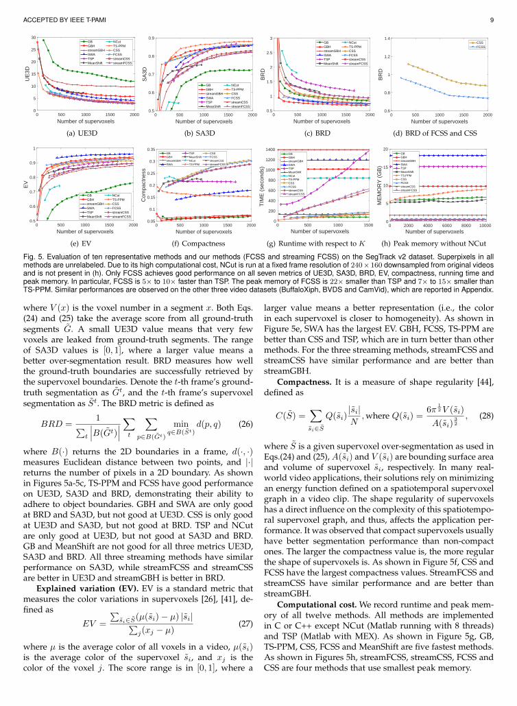
Fig. 5. Evaluation of ten representative methods and our methods (FCSS and streaming FCSS) on the SegTrack v2 dataset. Superpixels in allmethods are unrelabeled. Due to its high computational cost, NCut is run at a fixed frame resolution of 240×160 downsampled from original videosand is not present in (h). Only FCSS achieves good performance on all seven metrics of UE3D, SA3D, BRD, EV, compactness, running time andpeak memory. In particular, FCSS is 5× to 10× faster than TSP. The peak memory of FCSS is 22× smaller than TSP and 7× to 15× smaller thanTS-PPM. Similar performances are observed on the other three video datasets (BuffaloXiph, BVDS and CamVid), which are reported in Appendix.
where V (x) is the voxel number in a segment x. Both Eqs.(24) and (25) take the average score from all ground-truthsegments G. A small UE3D value means that very fewvoxels are leaked from ground-truth segments. The rangeof SA3D values is [0, 1], where a larger value means abetter over-segmentation result. BRD measures how wellthe ground-truth boundaries are successfully retrieved bythe supervoxel boundaries. Denote the t-th frame’s ground-truth segmentation as Gt, and the t-th frame’s supervoxelsegmentation as St. The BRD metric is defined as
BRD =1∑
t
∣∣∣B(Gt)∣∣∣∑t
∑p∈B(Gt)
minq∈B(St)
d(p, q) (26)
where B(·) returns the 2D boundaries in a frame, d(·, ·)measures Euclidean distance between two points, and |·|returns the number of pixels in a 2D boundary. As shownin Figures 5a-5c, TS-PPM and FCSS have good performanceon UE3D, SA3D and BRD, demonstrating their ability toadhere to object boundaries. GBH and SWA are only goodat BRD and SA3D, but not good at UE3D. CSS is only goodat UE3D and SA3D, but not good at BRD. TSP and NCutare only good at UE3D, but not good at SA3D and BRD.GB and MeanShift are not good for all three metrics UE3D,SA3D and BRD. All three streaming methods have similarperformance on SA3D, while streamFCSS and streamCSSare better in UE3D and streamGBH is better in BRD.
Explained variation (EV). EV is a standard metric thatmeasures the color variations in supervoxels [26], [41], de-fined as
EV =
∑si∈S(µ(si)− µ) |si|∑
j(xj − µ)(27)
where µ is the average color of all voxels in a video, µ(si)is the average color of the supervoxel si, and xj is thecolor of the voxel j. The score range is in [0, 1], where a
larger value means a better representation (i.e., the colorin each supervoxel is closer to homogeneity). As shown inFigure 5e, SWA has the largest EV. GBH, FCSS, TS-PPM arebetter than CSS and TSP, which are in turn better than othermethods. For the three streaming methods, streamFCSS andstreamCSS have similar performance and are better thanstreamGBH.
Compactness. It is a measure of shape regularity [44],defined as
C(S) =∑si∈S
Q(si)|si|N,where Q(si) =
6π12V (si)
A(si)32
, (28)
where S is a given supervoxel over-segmentation as used inEqs.(24) and (25),A(si) and V (si) are bounding surface areaand volume of supervoxel si, respectively. In many real-world video applications, their solutions rely on minimizingan energy function defined on a spatiotemporal supervoxelgraph in a video clip. The shape regularity of supervoxelshas a direct influence on the complexity of this spatiotempo-ral supervoxel graph, and thus, affects the application per-formance. It was observed that compact supervoxels usuallyhave better segmentation performance than non-compactones. The larger the compactness value is, the more regularthe shape of supervoxels is. As shown in Figure 5f, CSS andFCSS have the largest compactness values. StreamFCSS andstreamCSS have similar performance and are better thanstreamGBH.
Computational cost. We record runtime and peak mem-ory of all twelve methods. All methods are implementedin C or C++ except NCut (Matlab running with 8 threads)and TSP (Matlab with MEX). As shown in Figure 5g, GB,TS-PPM, CSS, FCSS and MeanShift are five fastest methods.As shown in Figures 5h, streamFCSS, streamCSS, FCSS andCSS are four methods that use smallest peak memory.

ACCEPTED BY IEEE T-PAMI 10
x
y
(even, even)
(even, odd)
(odd, even)
(odd, odd)
Fig. 6. For easy illustration, we present a superpixel example on a2D image. Assume 8-connectivity. For an arbitrary image with arbitraryground-truth segmentation, four unrelabeled superpixels are sufficient toachieve a perfect performance on the BRD metric, i.e., BRD = 0. Thesefour superpixels are characterized by the parity of the coordinates (x, y)of image pixels; i.e., the green, yellow, red and blue superpixels consistof pixels with coordinates (even, even), (even, odd), (odd, even) and(odd, odd), respectively.
Three more metrics – mean size variation (MSV), tem-poral extent (TEX) and label consistency (LC) – are usedin [41]. MSV and TEX measure the size variation and aver-age temporal extent of all supervoxels in a video. Since ourwork advocates to adapt the size of supervoxels accordingto video content density, these two metrics are no longersuitable. LC is evaluated using ground-truth optical flow.As aforementioned, optical flow is only a preprocessing toolto video applications and may introduce extra error intosupervoxel evaluation. In Section 7, we directly evaluatethese supervoxel methods in two video applications.
Comparison between unrelabeled and relabeled super-voxels. In the original implementation of the seven methodsin [41], a supervoxel label may be assigned to multiple dis-connected regions. We call such supervoxels unrelabeled. Un-relabeled supervoxels may lead to unexpected performanceon previous metrics; see Figure 6 for an (extreme) example.Then we further evaluate different supervoxel methods byrelabeling supervoxels such that each supervoxel is a simplyconnected region and each voxel is assigned to exactly onesupervoxel: we call such supervoxels relabeled. Relabelingsupervoxels only affect the number of supervoxels. It doesnot affect the visual appearance and functionality of su-pervoxels: if one object/region can be represented by theunion of a subset of unrelabeled supervoxels, it can alsobe represented by a subset of relabeled supervoxels. Aftersupervoxel relabeling, the isolated fragments with less thanτ voxels are merged with a randomly chosen neighboringsupervoxel. The performance of twelve supervoxel methodsafter relabeling with τ = 5, 10, 50, 100 are summarizedin Figure A5 in Appendix and the results with τ = 50are shown in Figure 7. The results show that only FCSS,streamFCSS, CSS, streamCSS, TSP and TS-PPM are insen-sitive to relabeling. Meanwhile, only FCSS achieves goodperformance on all five metrics of UE3D, SA3D, BRD, EVand compactness.
Comparison with TSP and TS-PPM. FCSS has similarUE3D, SA3D and EV performance with TSP and TS-PPM.FCSS has similar BRD performance with TS-PPM and isbetter than TSP. FCSS is much better in compactness thanboth TSP and TS-PPM. FCSS and TS-PPM are 5× to 10×faster than TSP. The peak memory of FCSS is 22× smallerthan TSP and 7× to 15× smaller than TS-PPM. Furthermore,in Section 7, we present two video applications and showthat FCSS achieves better results than TSP and TS-PPM.
Comparison with CSS. Both FCSS/streamFCSS and
0 2000 4000 6000 8000 10000
Number of supervoxels
0
5
10
15
20
25
30
UE
3D
GBGBHstreamGBHSWATSPMeanShift
NCutTS-PPMCSSFCSSstreamCSSstreamFCSS
(a) UE3D
0 2000 4000 6000 8000 10000
Number of supervoxels
0
0.2
0.4
0.6
0.8
1
SA
3D
GBGBHstreamGBHSWATSPMeanShift
NCutTS-PPMCSSFCSSstreamCSSstreamFCSS
(b) SA3D
0 2000 4000 6000 8000 10000
Number of supervoxels
0.4
0.5
0.6
0.7
0.8
0.9
1
1.1
BR
D
GBGBHstreamGBHSWATSPMeanShift
NCutTS-PPMCSSFCSSstreamCSSstreamFCSS
(c) BRD
0 2000 4000 6000 8000 10000
Number of supervoxels
0.6
0.7
0.8
0.9
1
1.1
BR
D
CSSFCSS
(d) BRD of FCSS and CSS
0 2000 4000 6000 8000 10000
Number of supervoxels
0.2
0.4
0.6
0.8
1
EV
GBGBHstreamGBHSWATSPMeanShift
NCutTS-PPMCSSFCSSstreamCSSstreamFCSS
(e) EV
0 2000 4000 6000 8000 10000
Number of supervoxels
0
0.1
0.2
0.3
0.4
0.5
Com
pact
ness
GBGBHstreamGBHSWA
TSPMeanShiftNCutTS-PPM
CSSFCSSstreamCSSstreamFCSS
(f) Compactness
Fig. 7. Evaluation of relabeled supervoxels on the SegTrack v2 dataset.Only FCSS achieves good performance on all five metrics of UE3D,SA3D, BRD, EV and compactness.
CSS/streamCSS use RCVT on video manifold M. Thanksto the feature-aware strategy by forcing cell centroids awayfrom video local boundaries, the FCSS method better finetunes the cell boundaries to align with the video localboundaries than CSS. As shown in Figure 5d and FigureA1 in Appendix, FCSS outperforms CSS on the metrics ofBRD, SA3D and EV, and has similar performance with CSSon UE3D. Meanwhile, FCSS is better than CSS in two novelvideo applications presented in Section 7.
7 APPLICATIONS
We evaluate the performance of various supervoxels inthe following two video applications. To faithfully comparedifferent supervoxel methods, we use their original settings,i.e., supervoxels are unrelabeled.
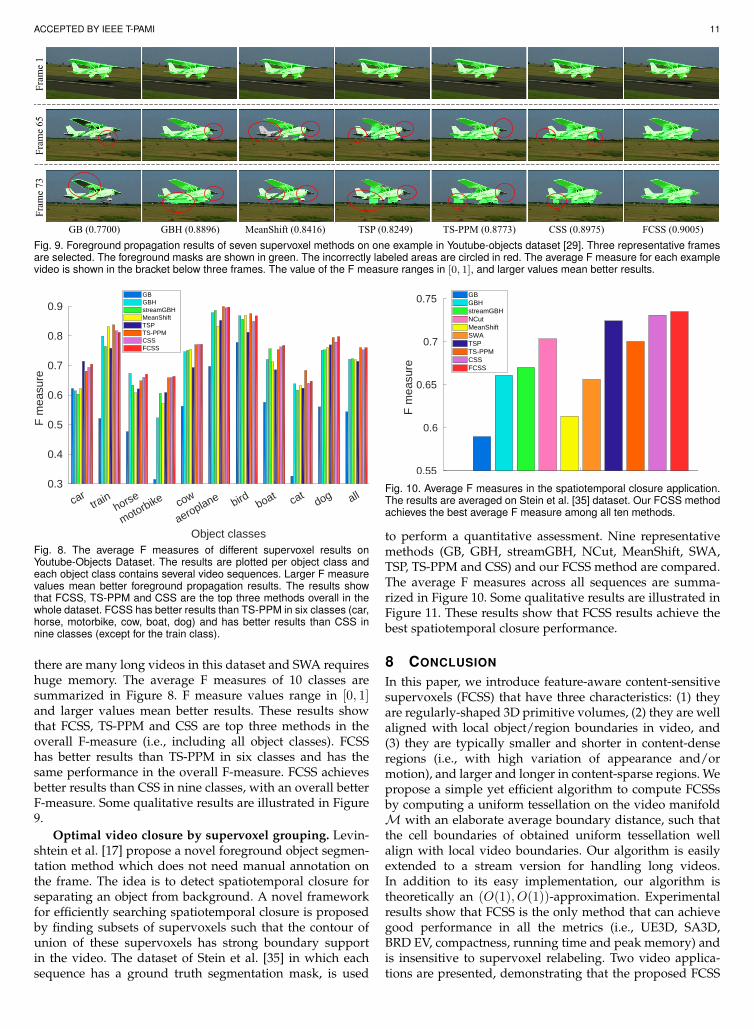
Foreground propagation in video. Given the first framewith manual annotation for the foreground object, a novelapproach is proposed in [14] to propagate the foregroundregion through time, with the aid of supervoxels to guideits estimates towards long-range coherent regions. Youtube-Objects dataset [29] (126 videos with 10 object classes) withforeground ground-truth, is used to perform a quantita-tive assessment. Seven representative methods (GB, GBH,streamGBH, MeanShift, TSP, TS-PPM and CSS) and ourFCSS method are compared. NCut is not compared dueto its high computational cost. SWA is not compared since
ACCEPTED BY IEEE T-PAMI 11
GB (0.7700) GBH (0.8896) MeanShift (0.8416) TSP (0.8249) TS-PPM (0.8773) CSS (0.8975) FCSS (0.9005)
Fram
e73
Fram
e65
Fram
e 1
Fig. 9. Foreground propagation results of seven supervoxel methods on one example in Youtube-objects dataset [29]. Three representative framesare selected. The foreground masks are shown in green. The incorrectly labeled areas are circled in red. The average F measure for each examplevideo is shown in the bracket below three frames. The value of the F measure ranges in [0, 1], and larger values mean better results.
cartra
inhorse
motorbike cow
aeroplane bird boat catdog all
Object classes
0.3
0.4
0.5
0.6
0.7
0.8
0.9
F m
easu
re
GBGBHstreamGBHMeanShiftTSPTS-PPMCSSFCSS
Fig. 8. The average F measures of different supervoxel results onYoutube-Objects Dataset. The results are plotted per object class andeach object class contains several video sequences. Larger F measurevalues mean better foreground propagation results. The results showthat FCSS, TS-PPM and CSS are the top three methods overall in thewhole dataset. FCSS has better results than TS-PPM in six classes (car,horse, motorbike, cow, boat, dog) and has better results than CSS innine classes (except for the train class).
there are many long videos in this dataset and SWA requireshuge memory. The average F measures of 10 classes aresummarized in Figure 8. F measure values range in [0, 1]and larger values mean better results. These results showthat FCSS, TS-PPM and CSS are top three methods in theoverall F-measure (i.e., including all object classes). FCSShas better results than TS-PPM in six classes and has thesame performance in the overall F-measure. FCSS achievesbetter results than CSS in nine classes, with an overall betterF-measure. Some qualitative results are illustrated in Figure9.
Optimal video closure by supervoxel grouping. Levin-shtein et al. [17] propose a novel foreground object segmen-tation method which does not need manual annotation onthe frame. The idea is to detect spatiotemporal closure forseparating an object from background. A novel frameworkfor efficiently searching spatiotemporal closure is proposedby finding subsets of supervoxels such that the contour ofunion of these supervoxels has strong boundary supportin the video. The dataset of Stein et al. [35] in which eachsequence has a ground truth segmentation mask, is used
0.55
0.6
0.65
0.7
0.75
F m
easu
re
GBGBHstreamGBHNCutMeanShiftSWATSPTS-PPMCSSFCSS
Fig. 10. Average F measures in the spatiotemporal closure application.The results are averaged on Stein et al. [35] dataset. Our FCSS methodachieves the best average F measure among all ten methods.
to perform a quantitative assessment. Nine representativemethods (GB, GBH, streamGBH, NCut, MeanShift, SWA,TSP, TS-PPM and CSS) and our FCSS method are compared.The average F measures across all sequences are summa-rized in Figure 10. Some qualitative results are illustrated inFigure 11. These results show that FCSS results achieve thebest spatiotemporal closure performance.
8 CONCLUSION
In this paper, we introduce feature-aware content-sensitivesupervoxels (FCSS) that have three characteristics: (1) theyare regularly-shaped 3D primitive volumes, (2) they are wellaligned with local object/region boundaries in video, and(3) they are typically smaller and shorter in content-denseregions (i.e., with high variation of appearance and/ormotion), and larger and longer in content-sparse regions. Wepropose a simple yet efficient algorithm to compute FCSSsby computing a uniform tessellation on the video manifoldM with an elaborate average boundary distance, such thatthe cell boundaries of obtained uniform tessellation wellalign with local video boundaries. Our algorithm is easilyextended to a stream version for handling long videos.In addition to its easy implementation, our algorithm istheoretically an (O(1), O(1))-approximation. Experimentalresults show that FCSS is the only method that can achievegood performance in all the metrics (i.e., UE3D, SA3D,BRD EV, compactness, running time and peak memory) andis insensitive to supervoxel relabeling. Two video applica-tions are presented, demonstrating that the proposed FCSS

ACCEPTED BY IEEE T-PAMI 12
Video Frame GB GBH MeanShift TSP TS-PPM CSS FCSS
0.2659 0.6891 0.4613 0.7399 0.7026 0.7405 0.7646
0.7031 0.7112 0.5717 0.7189 0.8059 0.7841 0.8163
0.8295 0.7588 0.8475 0.8458 0.8367 0.8906 0.9609
Fig. 11. Spatiotemporal closure results of seven supervoxel methods on three examples in Stein et al. dataset [35]. The optimal closure contoursare shown in red, and the boundaries of supervoxels are shown in green. One representative frame is illustrated for each video. The F measurevalue for each spatiotemporal closure is shown below each frame; the range of the F measure values is [0, 1], and larger values mean better results.
method can simultaneously achieve the best performancewith respect to various metrics.
REFERENCES
[1] N. Ailon, R. Jaiswal, and C. Monteleoni. Streaming k-meansapproximation. In Proceedings of the 22nd International Conference onNeural Information Processing Systems, NIPS’09, pages 10–18, 2009.
[2] D. Arthur and S. Vassilvitskii. K-means++: The advantages ofcareful seeding. In Proceedings of the Eighteenth Annual ACM-SIAMSymposium on Discrete Algorithms, SODA ’07, pages 1027–1035,2007.
[3] G. J. Brostow, J. Shotton, J. Fauqueur, and R. Cipolla. Segmentationand recognition using structure from motion point clouds. InEuropean Conference on Computer Vision, ECCV’08, pages 44–57.Springer, 2008.
[4] Y. Cai and X. Guo. Anisotropic superpixel generation based onmahalanobis distance. Computer Graphics Forum (Pacific Graphics2016), 35(7):199–207, 2016.
[5] J. Chang, D. Wei, and J. W. Fisher III. A video representation usingtemporal superpixels. In Proceedings of the 2013 IEEE Conference onComputer Vision and Pattern Recognition, CVPR ’13, pages 2051–2058, 2013.
[6] A. Y. Chen and J. J. Corso. Propagating multi-class pixel labelsthroughout video frames. In Proceedings of Western New York ImageProcessing Workshop, 2010.
[7] J. J. Corso, E. Sharon, S. Dube, S. El-Saden, U. Sinha, and A. L.Yuille. Efficient multilevel brain tumor segmentation with inte-grated Bayesian model classification. IEEE Trans. Med. Imaging,27(5):629–640, 2008.
[8] Q. Du, V. Faber, and M. Gunzburger. Centroidal Voronoi tessel-lations: Applications and algorithms. SIAM Review, 41(4):637–676,1999.
[9] P. F. Felzenszwalb and D. P. Huttenlocher. Efficient graph-basedimage segmentation. International Journal of Computer Vision,59(2):167–181, 2004.
[10] C. Fowlkes, S. Belongie, F. Chung, and J. Malik. Spectral groupingusing the nystrom method. IEEE Trans. Pattern Anal. Mach. Intell.,26(2):214–225, 2004.
[11] C. C. Fowlkes, S. J. Belongie, and J. Malik. Efficient spatiotemporalgrouping using the nystrom method. In 2001 IEEE ComputerSociety Conference on Computer Vision and Pattern Recognition, CVPR’01, pages 231–238, 2001.
[12] F. Galasso, N. S. Nagaraja, T. J. Cardenas, T. Brox, and B. Schiele. Aunified video segmentation benchmark: Annotation, metrics andanalysis. In Proceedings of the 2013 IEEE International Conference onComputer Vision, ICCV ’13, pages 3527–3534, 2013.
[13] M. Grundmann, V. Kwatra, M. Han, and I. A. Essa. Efficienthierarchical graph-based video segmentation. In IEEE Conferenceon Computer Vision and Pattern Recognition, CVPR’10, pages 2141–2148, 2010.
[14] S. D. Jain and K. Grauman. Supervoxel-consistent foregroundpropagation in video. In 13th European Conference on ComputerVision, ECCV’14, pages 656–671, 2014.
[15] Y. Ke, R. Sukthankar, and M. Hebert. Spatio-temporal shape andflow correlation for action recognition. In IEEE Computer SocietyConference on Computer Vision and Pattern Recognition, CVPR’07,2007.
[16] S. Lee, W. Jang, and C. Kim. Temporal superpixels based onproximity-weighted patch matching. In IEEE International Con-ference on Computer Vision, ICCV’17, pages 3630–3638, 2017.
[17] A. Levinshtein, C. Sminchisescu, and S. J. Dickinson. Optimalimage and video closure by superpixel grouping. InternationalJournal of Computer Vision, 100(1):99–119, 2012.
[18] A. Levinshtein, A. Stere, K. N. Kutulakos, D. J. Fleet, S. J. Dick-inson, and K. Siddiqi. Turbopixels: Fast superpixels using geo-metric flows. IEEE Trans. Pattern Analysis and Machine Intelligence,31(12):2290–2297, 2009.
[19] C. Li, L. Lin, W. Zuo, S. Yan, and J. Tang. SOLD: sub-optimallow-rank decomposition for efficient video segmentation. In IEEEConference on Computer Vision and Pattern Recognition, CVPR’15,pages 5519–5527, 2015.
[20] F. Li, T. Kim, A. Humayun, D. Tsai, and J. M. Rehg. Video segmen-tation by tracking many figure-ground segments. In Proceedingsof the IEEE International Conference on Computer Vision, ICCV’13,pages 2192–2199, 2013.
[21] Y. Liang, J. Shen, X. Dong, H. Sun, and X. Li. Video supervoxelsusing partially absorbing random walks. IEEE Trans. Circuits Syst.Video Techn., 26(5):928–938, 2016.
[22] M.-Y. Liu, O. Tuzel, S. Ramalingam, and R. Chellappa. Entropyrate superpixel segmentation. In IEEE Conference on ComputerVision and Pattern Recognition (CVPR ’11), pages 2097–2104, 2011.
[23] Y.-J. Liu, C. Yu, M. Yu, and Y. He. Manifold SLIC: a fast methodto compute content-sensitive superpixels. In IEEE Conference onComputer Vision and Pattern Recognition (CVPR 2016), pages 651–659, 2016.
[24] Y.-J. Liu, M. Yu, B.-J. Li, and Y. He. Intrinsic manifold SLIC:A simple and efficient method for computing content-sensitivesuperpixels. IEEE Trans. Pattern Anal. Mach. Intell., 40(3):653–666,2018.
[25] J. Lu, R. Xu, and J. J. Corso. Human action segmentation with hi-erarchical supervoxel consistency. In IEEE Conference on ComputerVision and Pattern Recognition, CVPR’15, pages 3762–3771, 2015.
[26] A. P. Moore, S. Prince, J. Warrell, U. Mohammed, and G. Jones. Su-perpixel lattices. In IEEE Computer Society Conference on ComputerVision and Pattern Recognition, CVPR ’08, 2008.
[27] D. Oneata, J. Revaud, J. Verbeek, and C. Schmid. Spatio-temporalobject detection proposals. In D. Fleet, T. Pajdla, B. Schiele, andT. Tuytelaars, editors, 13th European Conference on Computer Vision,ECCV’14, pages 737–752, 2014.
[28] S. Paris and F. Durand. A topological approach to hierarchical seg-mentation using mean shift. In IEEE Computer Society Conferenceon Computer Vision and Pattern Recognition, CVPR’07, 2007.
[29] A. Prest, C. Leistner, J. Civera, C. Schmid, and V. Ferrari. Learning

ACCEPTED BY IEEE T-PAMI 13
object class detectors from weakly annotated video. In IEEEConference on Computer Vision and Pattern Recognition, CVPR’12,pages 3282–3289. IEEE, 2012.
[30] M. Reso, J. Jachalsky, B. Rosenhahn, and J. Ostermann. Temporallyconsistent superpixels. In IEEE International Conference on ComputerVision (ICCV ’13), pages 385–392, 2013.
[31] M. Reso, J. Jachalsky, B. Rosenhahn, and J. Ostermann. Occlusion-aware method for temporally consistent superpixels. IEEE Trans.Pattern Anal. Mach. Intell., DOI:10.1109/TPAMI.2018.2832628,2019.
[32] E. Sharon, A. Brandt, and R. Basri. Fast multiscale image seg-mentation. In IEEE Conference on Computer Vision and PatternRecognition, CVPR ’00, pages 1070–1077, 2000.
[33] E. Sharon, M. Galun, D. Sharon, R. Basri, and A. Brandt. Hierarchyand adaptivity in segmenting visual scenes. Nature, 442(7104):810–813, 2006.
[34] J. Shi and J. Malik. Normalized cuts and image segmentation.IEEE Trans. Pattern Anal. Mach. Intell., 22(8):888–905, 2000.
[35] A. N. Stein, D. Hoiem, and M. Hebert. Learning to find objectboundaries using motion cues. In IEEE 11th International Conferenceon Computer Vision, ICCV 2007, pages 1–8, 2007.
[36] D. Sun, S. Roth, and M. J. Black. A quantitative analysis of currentpractices in optical flow estimation and the principles behindthem. International Journal of Computer Vision, 106(2):115–137, 2014.
[37] P. Sundberg, T. Brox, M. Maire, P. Arbelaez, and J. Malik. Occlusionboundary detection and figure/ground assignment from opticalflow. In IEEE Conference on Computer Vision and Pattern Recognition,CVPR’11, pages 2233–2240. IEEE, 2011.
[38] O. Veksler, Y. Boykov, and P. Mehrani. Superpixels and supervox-els in an energy optimization framework. In Europeon Conferenceon Computer Vision (ECCV 2010), pages 211–224, 2010.
[39] P. Wang, G. Zeng, R. Gan, J. Wang, and H. Zha. Structure-sensitivesuperpixels via geodesic distance. International Journal of ComputerVision, 103(1):1–21, 2013.
[40] D. Wei. A constant-factor bi-criteria approximation guarantee fork-means++. In Annual Conference on Neural Information ProcessingSystems (NIPS) 2016, pages 604–612, 2016.
[41] C. Xu and J. J. Corso. Libsvx: A supervoxel library and benchmarkfor early video processing. International Journal of Computer Vision,119(3):272–290, 2016.
[42] C. Xu, C. Xiong, and J. J. Corso. Streaming hierarchical videosegmentation. In Proceedings of the 12th European Conference onComputer Vision - Volume Part VI, ECCV’12, pages 626–639, 2012.
[43] R. Yi, Y. Liu, and Y. Lai. Content-sensitive supervoxels via uniformtessellations on video manifolds. In IEEE Conference on ComputerVision and Pattern Recognition, CVPR’18, pages 646–655, 2018.
[44] R. Yi, Y. Liu, and Y. Lai. Evaluation on the compactness ofsupervoxels. In IEEE International Conference on Image Processing,ICIP’18, pages 2212–2216, 2018.
[45] C.-P. Yu, H. Le, G. Zelinsky, and D. Samaras. Efficient videosegmentation using parametric graph partitioning. In IEEE Inter-national Conference on Computer Vision, ICCV’15, pages 3155–3163,2015.