Computational Geometry 37 (2007) 115–133

www.elsevier.com/locate/comgeo

Shortest monotone descent path problem in polyhedral terrain ✩

Sasanka Roy, Sandip Das, Subhas C. Nandy ∗

Advanced Computing and Microelectronics Unit, Indian Statistical Institute, Kolkata 700 108, India

Received 2 December 2005; received in revised form 3 June 2006; accepted 24 June 2006

Available online 18 September 2006

Communicated by R. Klein

Abstract

Given a polyhedral terrain with n vertices, the shortest monotone descent path problem deals with finding the shortest pathbetween a pair of points, called source (s) and destination (t) such that the path is constrained to lie on the surface of the terrain, andfor every pair of points p = (x(p), y(p), z(p)) and q = (x(q), y(q), z(q)) on the path, if dist(s,p) < dist(s, q) then z(p) � z(q),where dist(s,p) denotes the distance of p from s along the aforesaid path. This is posed as an open problem by Berg and Kreveld[M. de Berg, M. van Kreveld, Trekking in the Alps without freezing or getting tired, Algorithmica 18 (1997) 306–323]. We showthat for some restricted classes of polyhedral terrain, the optimal path can be identified in polynomial time.© 2006 Elsevier B.V. All rights reserved.

Keywords: Shortest path; Polyhedral terrain; Algorithm; Complexity

1. Introduction

The shortest path problem between two points s and t on the surface of an unweighted polyhedron is studiedextensively in the literature. Sharir and Schorr [19] presented an O(n3 logn) time algorithm for finding the geodesicshortest path between two points on the surface of a convex polyhedron with n vertices. Mitchell et al. [13] studiedthe generalized version of this problem where the restriction of convexity is removed. The time complexities of theproposed algorithms is O(n2 logn). After a long time Chen and Han [6] improved the time complexity to O(n2).Finally, the best known algorithm for producing the optimal solution was proposed by Kapoor [8]; the running timeof this algorithm is O(n log2 n). Two approximation algorithms for this problem were proposed by Varadarajan andAgarwal [20]; it can produce paths of length 7(1 + ε) × opt and 15(1 + ε) × opt respectively; opt is the length ofthe optimal path between s and t , and ε is an user specified degree of precession. The running times are respectivelyO(n5/3 log(5n/3)) and O(n8/5 log(8n/5)). For convex polyhedron, an approximation algorithm was proposed byAgarwal et al. [1], which produces (1 + ε) × opt solution, and runs in O(n/

√ε ) time. A simple linear time 2-

approximation algorithm for this problem is proposed by Hershberger and Suri [9].

✩ A preliminary version of this paper appeared in: Proc. of the 22nd Annual Symposium on Theoretical Aspects of Computer Science (STACS-2005), LNCS, vol. 3404, 2005, pp. 281–292.

* Corresponding author.E-mail address: nandysc@isical.ac.in (S.C. Nandy).

0925-7721/$ – see front matter © 2006 Elsevier B.V. All rights reserved.doi:10.1016/j.comgeo.2006.06.003

116 S. Roy et al. / Computational Geometry 37 (2007) 115–133

The first work on approximating the minimum cost path of the weighted polyhedral surface appeared in a seminalpaper by Mitchell and Papadimitrou [14]. It presents an (1 + ε)-approximation algorithm, that runs in O(n8 logn)

time. An implementable method for solving the minimum cost path problem was given by Mata and Mitchell [12],which formulates the problem as a graph search problem and assures a solution of length (1 + ε) × opt. The running

time of the algorithm is O(n3N2Wεw

), where W and w are respectively the maximum and minimum weights amongall the faces of the polyhedron. Efficient approximation algorithms are also available in [2,3,11,16,17]. The latestresult on this problem appeared in the work of Aleksandrov et al. [4]. It proposes an (1 + ε)-approximation algorithmthat runs in O(C(P ) n√

εlog n

εlog 1

ε) time, where n and ε are as defined earlier, and C(P ) captures the geometric

parameters and the weight of the faces of the polyhedron P .Several variations of the path finding problems in polyhedral terrain are studied by Berg and Kreveld [5]. Given a

polyhedral terrain T with n vertices, the proposed algorithm constructs a linear size data structure in O(n logn) timeand can efficiently answer the following queries:

Given a pair of points s and t on the surface of T , and an altitude (height) ξ , does there exist a path between s

and t such that for each point p on the path z(p) � ξ?

Given a pair of points s and t on T , determine the minimum total ascent/descent among the path(s) between s

and t , where the total ascent of a non-monotone path is defined in [5].

Recently an interesting variation of the shortest path problem in the context of a terrain is proposed by Mitchell andSharir [15], where the objective is to compute the L1-shortest path between a pair of given points, such that the pathis restricted to lie on or above a given polyhedral terrain with n faces. The proposed algorithm runs in O(n3 logn)

time. The same paper also studies another variation of the shortest path problem on a terrain like structure, where a setof n vertical walls parallel to the x-axis are given. Each wall is positioned on the xy-plane. The ith wall, is positionedat y = ai , and its top boundary (denoted by ei ) is a line of the form z = bix + ci , where ai , bi and ci are givenconstants, a1 < a2 < · · · < an. The objective is to report the L2-shortest path between a given pair of query points s

and t , where s < a1 and t > an. The problem is referred to as the L2-shortest path over walls. Note that the shortestpath is always monotone with respect to the y-axis, and it bends on the edges ei , i = 1,2, . . . , n. It is also proved thatthe shortest path from s to t is the concatenation of two sub-paths, one of them is monotone ascending and the secondone is monotone descending with respect to z-coordinate. The standard method of solving this problem involves apreprocessing phase which splits each edge ei into segments, and then defines the shortest path map [18], such thatthe optimal L2-path from s to t can be obtained by following an appropriate path in the map. In [15], it is proved thatthe size of the shortest path map is O(n2) in the worst case, but finding a polynomial time algorithm for constructingthe map is left as an open problem.

We address the problem of computing the shortest among all possible monotone descending paths (if at least onesuch path exists) between a pair of points on the surface of a polyhedral terrain. This is a long-standing open problemin the sense that no bound on the combinatorial or Euclidean length of the shortest monotone descent path betweena pair of points on the surface of a polyhedral terrain is available in the literature [5]. Some interesting observationsof the problem lead us to design efficient polynomial time algorithm for solving this problem in the following twospecial cases, where

1. our search domain is among all possible monotone descent paths from s to t which are constrained to pass througha sequence of faces such that each pair of consecutive faces are in convex position, and the objective is to identifythe shortest among such paths (see Section 4), and

2. given a sequence of pairwise adjacent faces having their boundaries parallel to each other (but the faces are notall necessarily in convex (respectively concave) position); the objective is to find the shortest monotone descentpath from s to t through that sequence of faces (see Section 5).

In Case 1, if the terrain contains n triangulated faces, the preprocessing of those faces need O(n2 logn) timeand O(n2) space, and the shortest monotone descent path query through a sequence of convex faces can be answeredin O(k + logn) time (provided such a path exists), where k is the number of faces through which the optimum pathpasses. In Case 2, if a sequence of n faces with their boundaries in parallel position is given, the shortest monotone

S. Roy et al. / Computational Geometry 37 (2007) 115–133 117

descent path from s to t through that face sequence can be computed in O(n logn) time. The solution technique forthis case indicates the hardness of handling the general terrain.

The problem is motivated from the agricultural applications where the objective is to lay a canal of minimum lengthfrom the source of water at the top of the mountain to the ground for irrigation purpose. Another application of Case 2can be observed in the design of fluid circulation systems in automobiles or refrigerator/air-condition machines.

2. Preliminaries

A terrain T is a polyhedral surface in R3 with a special property: the vertical line at any point on the xy-plane

intersects the surface of T at most once. Thus, the projections of all the faces of a terrain on the xy-plane are mutuallynon-intersecting at their interior. Each vertex p of the terrain is specified by a triple (x(p), y(p), z(p)). Without lossof generality, we assume that all the faces of the terrain are triangles, and the source point s is a vertex of the terrain.

Definition 1. [13] Let f and f ′ be a pair of faces of T sharing an edge e. The planar unfolding of face f ′ onto facef is the image of the points of f ′ when rotated about the line e onto the plane of f such that the points in f and thepoints in f ′ lie in two different sides of the edge e respectively (i.e., the faces f ′ and f become coplanar and they donot overlap after unfolding).

Let {f0, f1, . . . , fm} be a sequence of adjacent faces. The edge common to fi−1 and fi is ei . We define the planarunfolding with respect to the edge sequence E = {e1, e2, . . . , em} as follows: obtain the planar unfolding of face fm

onto face fm−1, then get the planar unfolding of the resulting plane onto fm−2, and so on; finally, get the planarunfolding of the entire resulting plane onto f0. From now onwards, this event will be referred to as U(E).

A path π(s, t) from a point s to a point t on the surface of the terrain is said to be a geodesic path if it entirelylies on the surface of the terrain, it is not self-intersecting, and in each face its intersection with the path π(s, t) is astraight line segment. The geodesic distance dist(p, q) between a pair of points p and q on π(s, t) is the length of thepath from p to q along π(s, t). The path πgeo(s, t) is said to be the geodesic shortest path if the distance between s

and t along πgeo(s, t) is minimum among all possible geodesic paths from s to t .

Lemma 1. [13] For a pair of points α and β , if πgeo(α,β) passes through an edge sequence E of a polyhedron, thenin the planar unfolding U(E), the path πgeo(α,β) is a straight line segment.

Definition 2. A path π(s, t) (z(s) � z(t)) on the surface of a terrain is a monotone descent path if for every pair ofpoints p,q ∈ π(s, t), dist(s,p) < dist(s, q) implies z(p) � z(q).

We will use πmd(p, q) and δ(p, q) to denote the shortest monotone descent path from p to q and its length,respectively. If p∗ and q∗ are the image of p and q respectively in the unfolded plane along an edge sequencetraversed by path πgeo(p, q), the path πgeo(p, q) corresponds to the line segment [p∗, q∗] in that unfolded plane, andit satisfies monotone descent property, then q is said to be straight line reachable from p in the unfolded plane. Insuch a case, πmd(p, q) = πgeo(p, q).

Remark 1. A monotone descent path between a pair of points s and t may not exist (Fig. 1(a)). Again, if monotonedescent path from s to t exists, then πmd(s, t) may not coincide with πgeo(s, t) (Fig. 1(b)).

Fig. 1. Justification of Remark 1.

118 S. Roy et al. / Computational Geometry 37 (2007) 115–133

Fig. 2. Proof of Lemma 3.

Lemma 2. If the shortest monotone decent path πmd(s, t) passes through a face f , then the intersection of πmd(s, t)

with the face f is line segment.

Proof. [By contradiction] Let the portion of πmd(s, t), which lies in face f , is not a single line segment. Let usconsider a pair of points p1,p2(∈ f ) on the path πmd(s, t) (with dist(s,p1) < dist(s,p2)) such that their joiningline segment does not coincide with an edge of πmd(s, t). Note that the line segment [p1,p2] satisfies the monotonedescent property, and its length is less than the length of the path from p1 to p2 along πmd(s, t). Hence we have acontradiction. �Lemma 3. Given a vertex s and a pair of points α and β on the terrain T , πmd(s,α) and πmd(s, β) cannot intersectexcept at some vertex of T . Moreover, if they intersect at a vertex v then the length of the subpath from s to v on bothπmd(s,α) and πmd(s, β) are same.

Proof. Let πmd(s,α) and πmd(s, β) intersect at a point γ , which is equidistant from s along both the paths πmd(s,α)

and πmd(s, β), otherwise one of these two paths cannot be optimum. Thus, the second part of the lemma follows. Weprove the first part by contradiction. We need to consider two cases: (i) γ is inside a face (say f ), and (ii) γ lies on anedge e which is adjacent to a pair of faces f and f ′.

In case (i) consider a very small circle centered at γ which completely lies inside the face f . The path πmd(s,α)

intersects the circle at two points b and d , and the path πmd(s, β) intersects the circle at a and c (see Fig. 2). Fromthe second part of the lemma, the length of the paths s ∼ b → γ → d ∼ α and s ∼ a → γ → d ∼ α are same, andboth are optimum paths (by the statement of the lemma). Now, consider the path s ∼ a → d ∼ α. Its length is lessthan both the paths mentioned above (by triangle inequality). Again, z(a) � z(γ ) � z(d) due to the fact that bothπmd(s,α) and πmd(s, β) are monotone descent. So, the path s ∼ a → d ∼ α is monotone descent also. Thus, we havea contradiction.

The case (ii) can be similarly handles by unfolding f onto f ′ and drawing the circle around γ in the unfoldedplane. �Definition 3. Given an arbitrary point p on the surface of the terrain T , the descent flow region of p (called DFR(p))is the region on the surface of T such that each point q ∈ DFR(p) is reachable from p through a monotone descentpath.

Given a polyhedral terrain T and a given point s ∈ T , we study the following problems:

P1: Construct DFR(s).P2: For a given query point t ∈ DFR(s) report πmd(s, t), and its length.

Problem P2 seems to be difficult in general. We identified the following two special cases where it can be solved inpolynomial time.

S. Roy et al. / Computational Geometry 37 (2007) 115–133 119

P2.1: For a given source point s, we can construct a data structure such that given any query point t ∈ DFR(s), we canidentify the shortest monotone descent path from s to t provided DFR(s) is convex (to be defined in Section 4).

P2.2: Given a sequence of faces {f0, f1, . . . , fm} of a polyhedral terrain (not necessarily convex/concave), if ei de-notes the edge separating fi−1 and fi , and the projections of the edges e1, e2, . . . , em on the XY -plane areparallel, then we can identify the monotone descent shortest path between a pair of points s ∈ f0 and t ∈ fm

through that sequence of faces.

3. Computation of DFR(s)

Given the source point s, if it lies on an edge e of a triangulated face, we add s with the vertex opposite to e in boththe faces adjacent to e. If s lies inside a triangulated face then we add s to all the three vertices of that face. Thus s

may always be considered as a vertex of the triangulated terrain.

Observation 1. If r is reachable from s using monotone descent path, then DFR(r) ⊆ DFR(s).

Observation 2. Let spq be a triangular face adjacent to the source s with z(p) � z(q). Now,

(i) if z(s) � z(q) then spq ⊆ DFR(s),(ii) if z(s) < z(p) then spq ∩ DFR(s) = φ (empty region), and

(iii) if z(p) � z(s) < z(q) then there exists a point r on the edge (p, q) (with z(r) = z(s)) such that spr ⊆ DFR(s),and srq ⊂ DFR(s). In this case, if z(p) = z(r), then spr degenerates to the line segment [s,p] (or equiva-lently [s, r]).

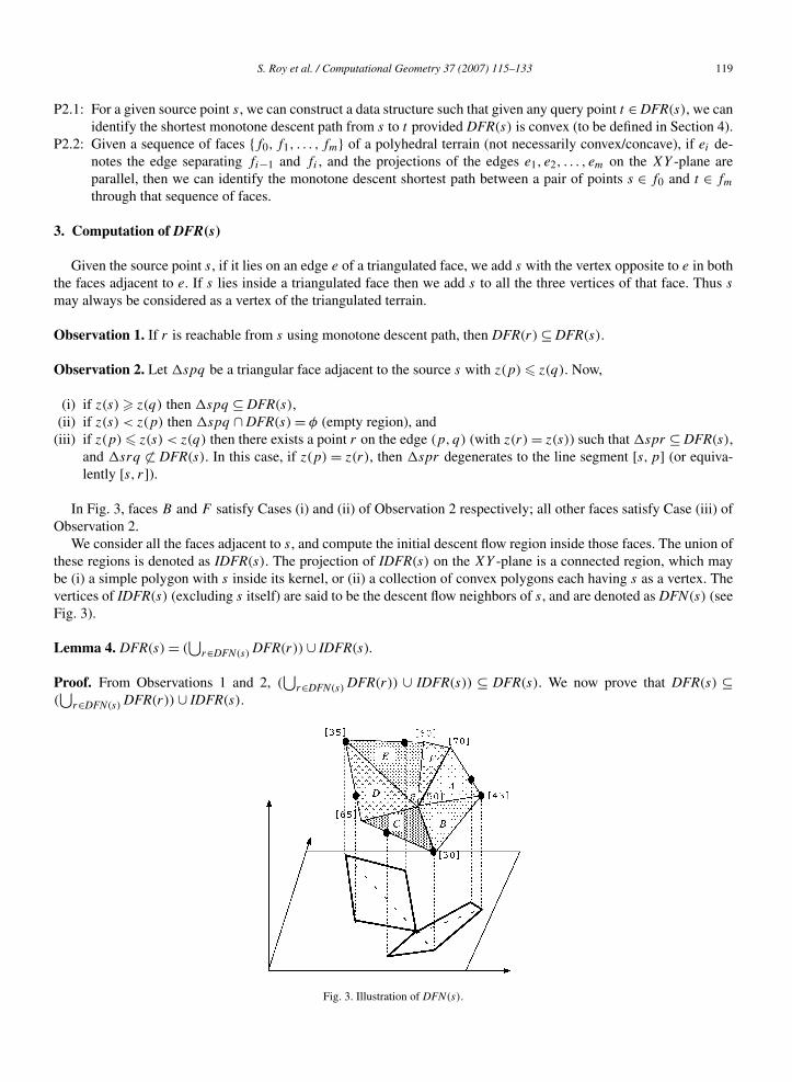
In Fig. 3, faces B and F satisfy Cases (i) and (ii) of Observation 2 respectively; all other faces satisfy Case (iii) ofObservation 2.

We consider all the faces adjacent to s, and compute the initial descent flow region inside those faces. The union ofthese regions is denoted as IDFR(s). The projection of IDFR(s) on the XY -plane is a connected region, which maybe (i) a simple polygon with s inside its kernel, or (ii) a collection of convex polygons each having s as a vertex. Thevertices of IDFR(s) (excluding s itself) are said to be the descent flow neighbors of s, and are denoted as DFN(s) (seeFig. 3).

Lemma 4. DFR(s) = (⋃

r∈DFN(s) DFR(r)) ∪ IDFR(s).

Proof. From Observations 1 and 2, (⋃

r∈DFN(s) DFR(r)) ∪ IDFR(s)) ⊆ DFR(s). We now prove that DFR(s) ⊆(⋃

r∈DFN(s) DFR(r)) ∪ IDFR(s).

Fig. 3. Illustration of DFN(s).

120 S. Roy et al. / Computational Geometry 37 (2007) 115–133

Fig. 4. DFR of a point α on an edge (a, b) where (a) z(c) > z(α) and (b) z(c) < z(α).

Fig. 5. Order of processing of the DFNs’.

Let q be a point in DFR(s) but not in (⋃

r∈DFN(s) DFR(r)) ∪ IDFR(s). Consider a monotone descent path from s

to q . By Observation 2, it intersects a boundary edge [a, b] of IDFR(s) at a point c. Assume that z(a) � z(b). Thepath from the point a to the point c along the boundary [a, b] is a monotone descent path. Thus, q ∈ DFR(a), whichleads to the contradiction. �

We compute IDFR(s) by considering the faces adjacent to s. The processing of the triangular faces which are notadjacent with the source s is discussed below.

Observation 3. If more than one point on the boundary of a face abc are reachable from s, then for each pair ofsuch points α and β , z(α) < z(β) implies DFR(α) ∩ abc ⊆ DFR(β) ∩ abc, and vice versa.

Observation 4. The intersection of a face of T with DFR(s) may be a vertex of that face, an edge of that face whichis parallel to XY -plane, or a polygonal region.

During the execution of the algorithm, we maintain a priority queue Q which is initialized with DFN(s), andprocess these elements in an ordered manner (as discussed below). During the processing of a member α ∈Q, the setof points DFN(α) are also inserted in Q. The algorithm continues until all the members in Q are processed.

While processing an element α ∈ Q, if it is a vertex of a triangular face abc, then it is processed as in Lemma 4.If it appears in the middle of an edge (a, b) (assuming z(a) > z(b)) then two situations may arise.

• If z(c) > z(α) then there exists a point β on the edge (b, c) with z(β) = z(α). Here, the triangular region bαβ

is included in DFR(s) (see Fig. 4(a)).• If z(c) < z(α) then there exists a point β on the edge (a, c) with z(β) = z(α). Here the quadrilateral �bαβc is

included in DFR(s) (see Fig. 4(b)).

In order to explain the order of processing of the elements in Q, let us consider a terrain in Fig. 5, the z-coordinatesof all the vertices are given in square bracket, and the DFN(s)’s are marked with dark circles. Now, consider thefollowing situations:

S. Roy et al. / Computational Geometry 37 (2007) 115–133 121

c is processed prior to b: Here, after processing of c, the region cbk is included in DFR(s), and generates thepoint k as a new DFN. After processing k, �kbgj is included in DFR(s). Next, when b is processed, bga isincluded in DFR(s) (see Fig. 5(a)).

b is processed prior to c: Here, after processing of b, abg, and bgh (⊂ bgi) are included in DFR(s). Now,if we process the point c then, as mentioned above, the �cbgj is included in DFR(s) (see Fig. 5(b)).

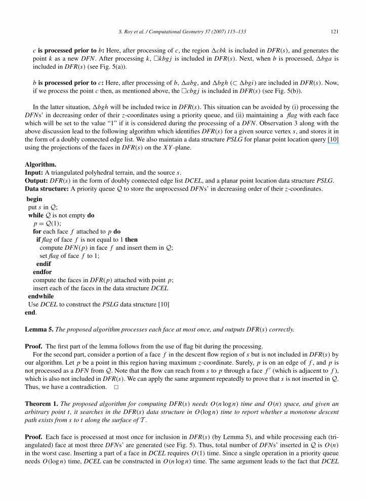
In the latter situation, bgh will be included twice in DFR(s). This situation can be avoided by (i) processing theDFNs’ in decreasing order of their z-coordinates using a priority queue, and (ii) maintaining a flag with each facewhich will be set to the value “1” if it is considered during the processing of a DFN. Observation 3 along with theabove discussion lead to the following algorithm which identifies DFR(s) for a given source vertex s, and stores it inthe form of a doubly connected edge list. We also maintain a data structure PSLG for planar point location query [10]using the projections of the faces in DFR(s) on the XY -plane.

Algorithm.Input: A triangulated polyhedral terrain, and the source s.Output: DFR(s) in the form of doubly connected edge list DCEL, and a planar point location data structure PSLG.Data structure: A priority queue Q to store the unprocessed DFNs’ in decreasing order of their z-coordinates.

beginput s in Q;while Q is not empty do

p = Q(1);for each face f attached to p doif flag of face f is not equal to 1 then

compute DFN(p) in face f and insert them in Q;set flag of face f to 1;

endifendforcompute the faces in DFR(p) attached with point p;insert each of the faces in the data structure DCEL

endwhileUse DCEL to construct the PSLG data structure [10]

end.

Lemma 5. The proposed algorithm processes each face at most once, and outputs DFR(s) correctly.

Proof. The first part of the lemma follows from the use of flag bit during the processing.For the second part, consider a portion of a face f in the descent flow region of s but is not included in DFR(s) by

our algorithm. Let p be a point in this region having maximum z-coordinate. Surely, p is on an edge of f , and p isnot processed as a DFN from Q. Note that the flow can reach from s to p through a face f ′ (which is adjacent to f ),which is also not included in DFR(s). We can apply the same argument repeatedly to prove that s is not inserted in Q.Thus, we have a contradiction. �Theorem 1. The proposed algorithm for computing DFR(s) needs O(n logn) time and O(n) space, and given anarbitrary point t , it searches in the DFR(s) data structure in O(logn) time to report whether a monotone descentpath exists from s to t along the surface of T .

Proof. Each face is processed at most once for inclusion in DFR(s) (by Lemma 5), and while processing each (tri-angulated) face at most three DFNs’ are generated (see Fig. 5). Thus, total number of DFNs’ inserted in Q is O(n)

in the worst case. Inserting a part of a face in DCEL requires O(1) time. Since a single operation in a priority queueneeds O(logn) time, DCEL can be constructed in O(n logn) time. The same argument leads to the fact that DCEL

122 S. Roy et al. / Computational Geometry 37 (2007) 115–133

needs O(n) space. Given the DCEL, the PSLG data structure can also be constructed in O(n logn) time using O(n)

space [10]. The query time complexity in PSLG is O(logn) [10]. �4. Shortest monotone descent path in convex DFR

We now study a restricted version of the descent flow problem where DFR(s) is convex.

Definition 4. Let f and f ′ be two adjacent faces of the terrain T sharing an edge e. Let p and q be two points on facesf and f ′ respectively (none of p and q is on e). Now, if the line segment [p,q] is not visible (respectively visible)from the outside of the terrain then f and f ′ are said to be in convex (respectively concave) position.

Definition 5. Given a terrain T and a source point s, DFR(s) is said to be convex if every two adjacent faces in DFR(s)

is in convex position. Similarly, DFR(s) is said to be concave if its every pair of adjacent faces is in concave position.

We now study the properties of shortest monotone descent path in a convex DFR(s). The convexity of DFR(s) canbe tested very easily by observing the neighbors of its each face. From now onwards, we assume that the DFR(s) onwhich we are working, is convex.

Observation 5. If p1,p2 are two points on a face of T , and p3 is another point on the line segment [p1,p2], thenz(p1) > z(p3) implies z(p2) < z(p3).

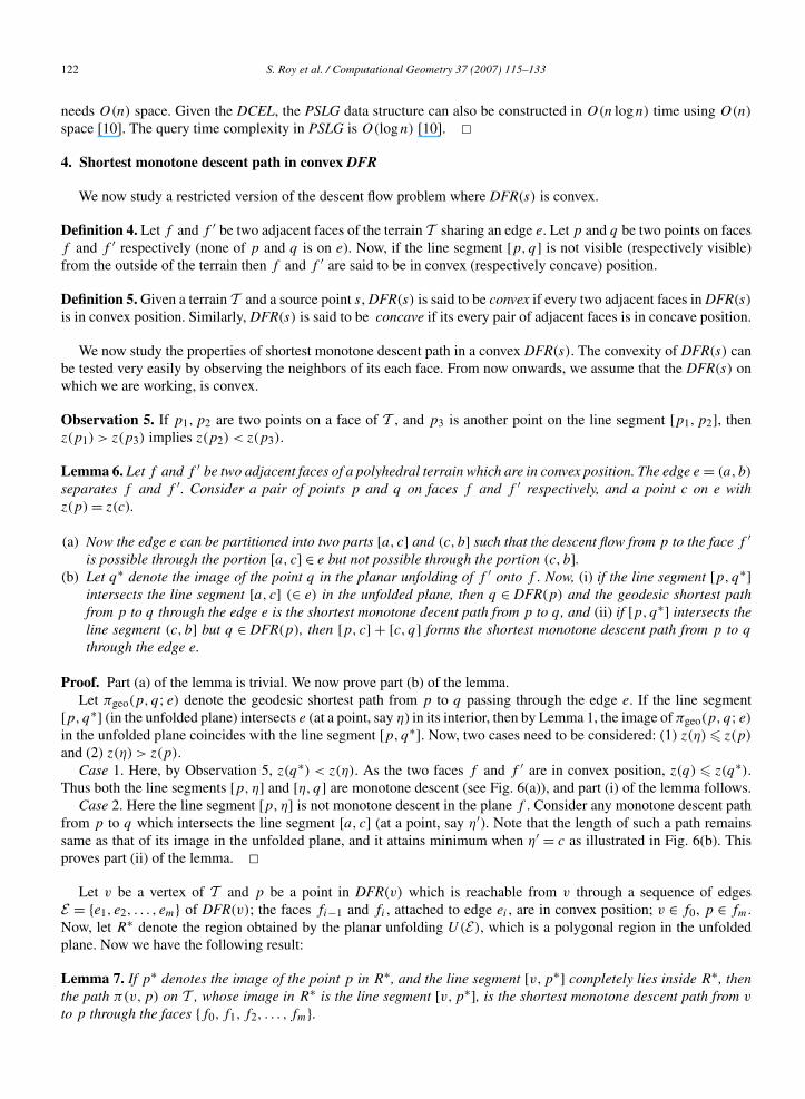
Lemma 6. Let f and f ′ be two adjacent faces of a polyhedral terrain which are in convex position. The edge e = (a, b)

separates f and f ′. Consider a pair of points p and q on faces f and f ′ respectively, and a point c on e withz(p) = z(c).

(a) Now the edge e can be partitioned into two parts [a, c] and (c, b] such that the descent flow from p to the face f ′is possible through the portion [a, c] ∈ e but not possible through the portion (c, b].

(b) Let q∗ denote the image of the point q in the planar unfolding of f ′ onto f . Now, (i) if the line segment [p,q∗]intersects the line segment [a, c] (∈ e) in the unfolded plane, then q ∈ DFR(p) and the geodesic shortest pathfrom p to q through the edge e is the shortest monotone decent path from p to q , and (ii) if [p,q∗] intersects theline segment (c, b] but q ∈ DFR(p), then [p, c] + [c, q] forms the shortest monotone descent path from p to q

through the edge e.

Proof. Part (a) of the lemma is trivial. We now prove part (b) of the lemma.Let πgeo(p, q; e) denote the geodesic shortest path from p to q passing through the edge e. If the line segment

[p,q∗] (in the unfolded plane) intersects e (at a point, say η) in its interior, then by Lemma 1, the image of πgeo(p, q; e)in the unfolded plane coincides with the line segment [p,q∗]. Now, two cases need to be considered: (1) z(η) � z(p)

and (2) z(η) > z(p).Case 1. Here, by Observation 5, z(q∗) < z(η). As the two faces f and f ′ are in convex position, z(q) � z(q∗).

Thus both the line segments [p,η] and [η,q] are monotone descent (see Fig. 6(a)), and part (i) of the lemma follows.Case 2. Here the line segment [p,η] is not monotone descent in the plane f . Consider any monotone descent path

from p to q which intersects the line segment [a, c] (at a point, say η′). Note that the length of such a path remainssame as that of its image in the unfolded plane, and it attains minimum when η′ = c as illustrated in Fig. 6(b). Thisproves part (ii) of the lemma. �

Let v be a vertex of T and p be a point in DFR(v) which is reachable from v through a sequence of edgesE = {e1, e2, . . . , em} of DFR(v); the faces fi−1 and fi , attached to edge ei , are in convex position; v ∈ f0, p ∈ fm.Now, let R∗ denote the region obtained by the planar unfolding U(E), which is a polygonal region in the unfoldedplane. Now we have the following result:

Lemma 7. If p∗ denotes the image of the point p in R∗, and the line segment [v,p∗] completely lies inside R∗, thenthe path π(v,p) on T , whose image in R∗ is the line segment [v,p∗], is the shortest monotone descent path from v

to p through the faces {f0, f1, f2, . . . , fm}.

S. Roy et al. / Computational Geometry 37 (2007) 115–133 123

Fig. 6. Proof of Lemma 6.

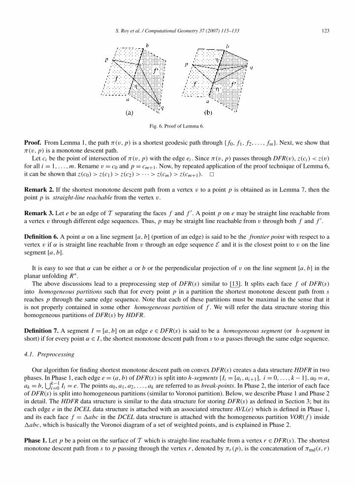
Proof. From Lemma 1, the path π(v,p) is a shortest geodesic path through {f0, f1, f2, . . . , fm}. Next, we show thatπ(v,p) is a monotone descent path.

Let ci be the point of intersection of π(v,p) with the edge ei . Since π(v,p) passes through DFR(v), z(ci) < z(v)

for all i = 1, . . . ,m. Rename v = c0 and p = cm+1. Now, by repeated application of the proof technique of Lemma 6,it can be shown that z(c0) > z(c1) > z(c2) > · · · > z(cm) > z(cm+1). �Remark 2. If the shortest monotone descent path from a vertex v to a point p is obtained as in Lemma 7, then thepoint p is straight-line reachable from the vertex v.

Remark 3. Let e be an edge of T separating the faces f and f ′. A point p on e may be straight line reachable froma vertex v through different edge sequences. Thus, p may be straight line reachable from v through both f and f ′.

Definition 6. A point α on a line segment [a, b] (portion of an edge) is said to be the frontier point with respect to avertex v if α is straight line reachable from v through an edge sequence E and it is the closest point to v on the linesegment [a, b].

It is easy to see that α can be either a or b or the perpendicular projection of v on the line segment [a, b] in theplanar unfolding R∗.

The above discussions lead to a preprocessing step of DFR(s) similar to [13]. It splits each face f of DFR(s)

into homogeneous partitions such that for every point p in a partition the shortest monotone descent path from s

reaches p through the same edge sequence. Note that each of these partitions must be maximal in the sense that itis not properly contained in some other homogeneous partition of f . We will refer the data structure storing thishomogeneous partitions of DFR(s) by HDFR.

Definition 7. A segment I = [a, b] on an edge e ∈ DFR(s) is said to be a homogeneous segment (or h-segment inshort) if for every point α ∈ I , the shortest monotone descent path from s to α passes through the same edge sequence.

4.1. Preprocessing

Our algorithm for finding shortest monotone descent path on convex DFR(s) creates a data structure HDFR in twophases. In Phase 1, each edge e = (a, b) of DFR(s) is split into h-segments {Ii = [ai, ai+1], i = 0, . . . , k − 1}, a0 = a,ak = b,

⋃k−1i=0 Ii = e. The points a0, a1, a2, . . . , ak are referred to as break-points. In Phase 2, the interior of each face

of DFR(s) is split into homogeneous partitions (similar to Voronoi partition). Below, we describe Phase 1 and Phase 2in detail. The HDFR data structure is similar to the data structure for storing DFR(s) as defined in Section 3; but itseach edge e in the DCEL data structure is attached with an associated structure AVL(e) which is defined in Phase 1,and its each face f = abc in the DCEL data structure is attached with the homogeneous partition VOR(f ) insideabc, which is basically the Voronoi diagram of a set of weighted points, and is explained in Phase 2.

Phase 1. Let p be a point on the surface of T which is straight-line reachable from a vertex r ∈ DFR(s). The shortestmonotone descent path from s to p passing through the vertex r , denoted by πr(p), is the concatenation of πmd(s, r)

124 S. Roy et al. / Computational Geometry 37 (2007) 115–133

Fig. 7. Processing a point v which is not a vertex of DFR(s).

and the line segment [r,p]. Its length is δr (p) = δ(s, r)+dist(r,p). Here dist(r,p) is equal to the length of the straightline segment [r,p∗] in the unfolded plane.

Definition 8. Let I = [a, b] be an h-segment on an edge e such that πmd(s,α) = πr(α) for every point α ∈ I , then thevertex r is said to be the link-vertex for the h-segment I .

The end points of the h-segments are referred to as break-points. If r is the link-vertex of a h-segment I , and E ={e1, e2, . . . , em} be the edge sequence which are intersected by the line segment [r,α] for every point α ∈ I , then thelast edge em in E is called the predecessor of I in the HDFR data structure. If [r,α] does not intersect any edge, thenthe predecessor of I is r itself. Then we have the following remarks.

If ai is a break-point on an edge e, and is shared by two h-segments [ai−1, ai] and [ai, ai+1] with link vertices r

and u respectively, then δr (ai) = δu(ai).

If I1 = [a1, b1] and I2 = [a2, b2] are two h-segments on an edge e (adjacent to faces f and f ′) with link-vertex r1and r2 respectively, and both I1 and I2 are reachable from r1 and r2 respectively through the same face f , then I1and I2 have mutually disjoint interiors.

Thus, the h-segments generated on an edge e are non-overlapping, and can be orderly maintained in an AVL-tree,named as AVL(e). We also need to compute the frontier-point on each h-segment [a, b] with respect to its link-vertex.Each h-segment is attached with its (i) predecessor, (ii) link-vertex, and (iii) three pointers, namely ptr1, ptr2 and ptr3,which will point to three elements of MIN-HEAP data structure corresponding to the two break-points and the frontierpoint of that h-segment. A vertex of DFR(s) in the HDFR data structure is also attached with its predecessor and link-vertex, which can be defined in a manner similar to the h-segments.

During the execution of the HDFR creation algorithm, we use a MIN_HEAP containing all the vertices, break-points and frontier-points explored so far. Each element α in the MIN_HEAP is attached with δ(s,α) (explored sofar), and a pointer field, called self_ptr. The self_ptr points to the h-segments in the HDFR, that has introduced thepoint α in the MIN_HEAP. Execution starts by putting s in MIN_HEAP with δ(s, s) = 0, and proceeds in a mannersimilar to Dijkstra’s shortest path algorithm. But, unlike Dijkstra’s algorithm, here the event-points are generatedduring the execution and are inserted in the MIN_HEAP. For each element in the MIN_HEAP, the monotone descentpath from s exists, but there is a possibility of obtaining an alternate path of smaller length. The exception holds forthe root node (say v) of the MIN_HEAP, whose attached δ-value cannot be reduced further by choosing an alternatemonotone descent path.

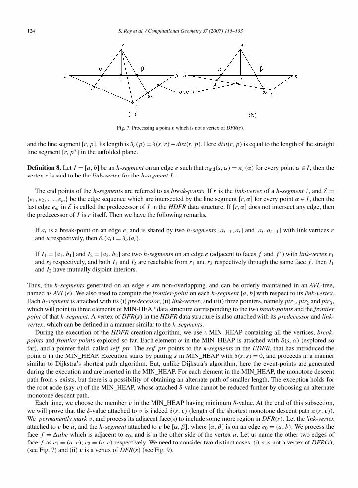
Each time, we choose the member v in the MIN_HEAP having minimum δ-value. At the end of this subsection,we will prove that the δ-value attached to v is indeed δ(s, v) (length of the shortest monotone descent path π(s, v)).We permanently mark v, and process its adjacent face(s) to include some more region in DFR(s). Let the link-vertexattached to v be u, and the h-segment attached to v be [α,β], where [α,β] is on an edge e0 = (a, b). We process theface f = abc which is adjacent to e0, and is in the other side of the vertex u. Let us name the other two edges offace f as e1 = (a, c), e2 = (b, c) respectively. We need to consider two distinct cases: (i) v is not a vertex of DFR(s),(see Fig. 7) and (ii) v is a vertex of DFR(s) (see Fig. 9).

S. Roy et al. / Computational Geometry 37 (2007) 115–133 125

Fig. 8. Overlaps of I with other h-segments.

Case (i): v is not a vertex of DFR(s)

Let R be the planar unfolding of all the faces intersected by the path π(u, v). We unfold face f onto R, join (u,α)

and (u,β) and extend these lines inside face f . These lines hit the boundary of f at μ and ω respectively. Let I bethe portion of the boundary of f from μ to ω, which is straight-line reachable from u in the planar unfolding R.I contributes one or two h-segments in the HDFR depending on whether it is a single interval (on either e1 or e2)or contains the vertex c (see Figs. 7(a) and 7(b) respectively). We compute δu(μ) and δu(ω) and search the interval[μ,ω] in the AVL(e) attached to the edge e in the HDFR data structure.

If I does not overlap with the existing h-segments then we (i) insert the h-segment [μ,ω] in AVL(e), (ii) insert μ

and ω in the MIN_HEAP with respect to δu(μ) and δu(ω) respectively, (iii) insert the frontier-point φ ∈ [μ,ω] (withrespect to δu(φ)) if it does not coincide with any of μ and ω, and (iv) set the self_ptr of μ, ω and φ to point I = [μ,ω]in the HDFR data structure.

If I overlaps with the h-segments {Ji = [φi,ψi], i = 1, . . . , k}, k � 1 on an edge e, μ ∈ J1 and ω ∈ Jk (seeFig. 8(a)), and the link-vertex attached to Ji is ri , then we consider each interval Ji, i = 1,2, . . . , k in order. For eachJi , we compute δri (φi), δri (ψi), δu(φi) and δu(ψi). Depending on the relationship among these four quantities, wemay have to replace Ji in AVL(e) by some newly generated h-segments as described below. The same technique wasfollowed in [13]. If Ji = [φi,ψi] needs to be replaced then we split it two or three pieces depending on the followingsituations:

Case 1. μ ∈ [φi,ψi] but ω /∈ [φi,ψi]: Here Ji splits into two pieces, namely J1i = [φi,μ] and J2i = [μ,ψi](see Fig. 8(b)).

Case 2. μ,ω ∈ [φi,ψi]: Here Ji splits into three pieces, namely J1i = [φi,μ], J2i = [μ,ω] and J3i = [ω,ψi](see Fig. 8(c)).

Case 3. μ /∈ [φi,ψi] but ω ∈ [φi,ψi]: Here Ji splits into two pieces, namely J2i = [φi,ω] and J3i = [ω,ψi](see Fig. 8(d)).

In either of these situations, we identify the tie-point τ ∈ J2i (see p. 658 of [13]), where δri (τ ) = δu(τ ) (if it exists).If the tie-point (τ ) is found, then it splits J2i into two intervals. Finally, we delete Ji and insert all the newly generated

126 S. Roy et al. / Computational Geometry 37 (2007) 115–133

Fig. 9. Processing a vertex.

h-segments (with their corresponding predecessors and link-vertices) in the HDFR data structure, where

deletion of a h-segment from an edge e implies its removal from AVL(e), and deletion of its two break-points andone frontier-point (if it exists) from MIN-HEAP. These three elements in the MIN-HEAP are accessed using ptr1,ptr2 and ptr3 attached to that h-segment, and

insertion of a h-segment on an edge e implies its insertion in AVL(e), setting the link-vertex, predecessor, andself_ptr of its two break-points and the frontier-point (if it is different from one of its break-points), and finallyinserting these two/three elements in the MIN-HEAP. Finally, the ptr1, ptr2 and ptr3 of the h-segment are set topoint these three elements in the MIN-HEAP.

After processing all the Jis’ for i = 1,2, . . . , k, we replace all the h-segments in AVL(e) having the same link-vertexu by a single h-segment which is obtained by merging them.

If the above steps are executed for at least one Ji , then we insert μ (or the corresponding tie-point) and ω (or thecorresponding tie-point) as break-points in the MIN_HEAP along with their respective δ-values and self_ptr. For eachnewly inserted h-segment the corresponding frontier-point is also to be inserted in MIN_HEAP.

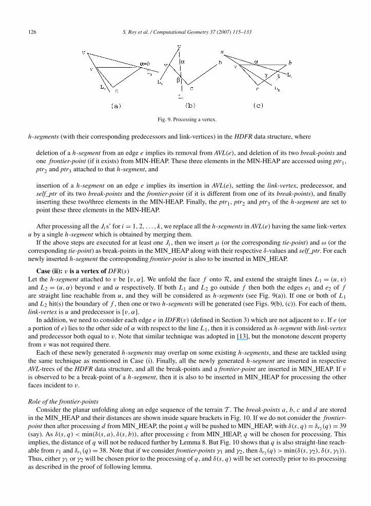
Case (ii): v is a vertex of DFR(s)

Let the h-segment attached to v be [v,α]. We unfold the face f onto R, and extend the straight lines L1 = (u, v)

and L2 = (u,α) beyond v and α respectively. If both L1 and L2 go outside f then both the edges e1 and e2 of f

are straight line reachable from u, and they will be considered as h-segments (see Fig. 9(a)). If one or both of L1and L2 hit(s) the boundary of f , then one or two h-segments will be generated (see Figs. 9(b), (c)). For each of them,link-vertex is u and predecessor is [v,α].

In addition, we need to consider each edge e in IDFR(v) (defined in Section 3) which are not adjacent to v. If e (ora portion of e) lies to the other side of α with respect to the line L1, then it is considered as h-segment with link-vertexand predecessor both equal to v. Note that similar technique was adopted in [13], but the monotone descent propertyfrom v was not required there.

Each of these newly generated h-segments may overlap on some existing h-segments, and these are tackled usingthe same technique as mentioned in Case (i). Finally, all the newly generated h-segment are inserted in respectiveAVL-trees of the HDFR data structure, and all the break-points and a frontier-point are inserted in MIN_HEAP. If v

is observed to be a break-point of a h-segment, then it is also to be inserted in MIN_HEAP for processing the otherfaces incident to v.

Role of the frontier-pointsConsider the planar unfolding along an edge sequence of the terrain T . The break-points a, b, c and d are stored

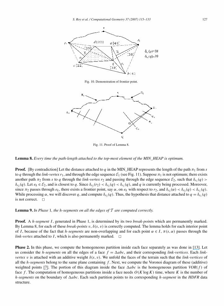
in the MIN_HEAP and their distances are shown inside square brackets in Fig. 10. If we do not consider the frontier-point then after processing d from MIN_HEAP, the point q will be pushed to MIN_HEAP, with δ(s, q) = δr2(q) = 39(say). As δ(s, q) < min(δ(s, a), δ(s, b)), after processing c from MIN_HEAP, q will be chosen for processing. Thisimplies, the distance of q will not be reduced further by Lemma 8. But Fig. 10 shows that q is also straight-line reach-able from r1 and δr1(q) = 38. Note that if we consider frontier-points γ1 and γ2, then δr2(q) > min(δ(s, γ2), δ(s, γ1)).Thus, either γ1 or γ2 will be chosen prior to the processing of q , and δ(s, q) will be set correctly prior to its processingas described in the proof of following lemma.

S. Roy et al. / Computational Geometry 37 (2007) 115–133 127

Fig. 10. Demonstration of frontier point.

Fig. 11. Proof of Lemma 8.

Lemma 8. Every time the path-length attached to the top-most element of the MIN_HEAP is optimum.

Proof. [By contradiction] Let the distance attached to q in the MIN_HEAP represents the length of the path π1 from s

to q through the link-vertex r1, and through the edge sequence E1 (see Fig. 11). Suppose π1 is not optimum; there existsanother path π2 from s to q through the link-vertex r2 and passing through the edge sequence E2, such that δr1(q) >

δr2(q). Let ek ∈ E2, and is closest to q . Since δr2(r2) < δr2(q) < δr1(q), and q is currently being processed. Moreover,since π2 passes through ek , there exists a frontier point, say α, on ek with respect to r2, and δr2(α) < δr2(q) < δr1(q).While processing α, we will discover q , and compute δr2(q). Thus, the hypothesis that distance attached to q = δr1(q)

is not correct. �Lemma 9. In Phase 1, the h-segments on all the edges of T are computed correctly.

Proof. A h-segment I , generated in Phase 1, is determined by its two break-points which are permanently marked.By Lemma 8, for each of these break-points v, δ(s, v) is correctly computed. The lemma holds for each interior pointof I , because of the fact that h-segments are non-overlapping and for each point α ∈ I , π(s,α) passes through thelink-vertex attached to I , which is also permanently marked. �Phase 2. In this phase, we compute the homogeneous partition inside each face separately as was done in [13]. Letus consider the h-segments on all the edges of a face f = abc, and their corresponding link-vertices. Each link-vertex v is attached with an additive weight δ(s, v). We unfold the faces of the terrain such that the link-vertices ofall the h-segments belong to the same plane containing f . Next, we compute the Voronoi diagram of these (additive)weighted points [7]. The portion of this diagram inside the face abc is the homogeneous partition VOR(f ) offace f . The computation of homogeneous partitions inside a face needs O(K logK) time, where K is the number ofh-segments on the boundary of abc. Each such partition points to its corresponding h-segment in the HDFR datastructure.

128 S. Roy et al. / Computational Geometry 37 (2007) 115–133

4.2. Query answering

For a given query point t , we first locate the face f = abc of DFR(s) containing t . Next, we need to search inthe data structure VOR(f ) to decide the appropriate cell inside f in which the query point lies. This actually givesthe h-segment I through which the shortest path from s to t has entered that face, and the length of the correspondingpath (see Theorem 3). We use predecessor links to obtain the edge sequence E∗ = {e∗

1, e∗2, . . . , e∗

m}, to reach the link-vertex r (a vertex of DFR(s)) attached to I . Thus, the shortest monotone descent path π(r, t) passes through facesf ∗

0 , f ∗1 , f ∗

2 , . . . , f ∗m = f , where r is a vertex of f ∗

0 , and t ∈ f ∗m, and the edge e∗

i is shared by f ∗i−1 and f ∗

i . Finally, weobtain the entire path π(s, t) using the following steps.

• Compute π(r, t) through the edge sequence E∗ as mentioned above.• From r , reach its link-vertex r1 through an edge sequence obtained using predecessor pointers. Compute the

planar unfolding of the faces, adjacent to that edge sequence. The inverse image of the line segment [r1, r] in theunfolded plane is the shortest descent flow path from r1 to r .

• Treat r1 as r , and repeat step (ii) until the vertex s is reached.

4.3. Complexity analysis

The total number of vertices and edges in DFR(s) are both O(n). Let us consider the h-segments on an edge e

coming through one of its adjacent faces. Each such h-segment is designated by two lines originating from its linkvertex and is supported by some other vertex of T . Note that one vertex cannot support more than one such lines.Thus, the number of h-segments on an edge of T is O(n) in the worst case. The final set of h-segments on an edgeis obtained by merging the two sets of h-segments coming through its two adjacent faces, which is also O(n). Eachh-segment is attached with a frontier-point. Thus, the total number of event-points pushed in the MIN_HEAP maybe O(n2) in the worst case. Processing of all these event-points needs O(n2 logn) time. Finally, in Phase 2, the timecomplexity of computing the homogeneous partitioning of all the faces is O(n2 logn) in total, and it produces O(n2)

homogeneous partitions. The worst case size of the HDFR is O(n2).The query time needs O(logn + k), where O(logn) time is required for the point location queries with the query

point t as mentioned in Subsection 4.2, and k is the number of line segments on the shortest path from s to t . Thus wehave the following theorem:

Theorem 2. Given a convex DFR(s) of a polyhedral terrain T with n vertices, and a source point s, our algorithm(i) creates the HDFR data structure in O(n2 logn) time and O(n2) space. (ii) For a given query point t ∈ DFR(s),it outputs a monotone descent path from s to t in O(k + logn) time, where k is the number of line segments on theoptimal path.

4.4. A simple variation: the distance query

A simpler version of the above problem is the distance query, where the objective is to compute the length of themonotone descent path from s to a given query point t . We show that a minor tailoring of the HDFR data structurehelps us to report the length in O(logn) time.

Recall the Phase 2 of the preprocessing. Here, we have assumed that the length of the shortest path of each link-vertex is already known. At each face, we have considered the link-vertices attached to the h-segments on its boundaryas weighted points, where the weight attached to a link vertex is the length of the shortest monotone descent pathfrom s to that point. Next, we computed the Voronoi diagram of those weighted points inside that face. At eachpartition, we attach two scalar information: (i) the coordinate of the image of its corresponding link-vertex in theunfolded plane, and (ii) the distance of that link-vertex from s.

During the distance query for a query point t , we identify the partition in which it belongs by point location. Letr be the link-vertex attached to that partition. The length of the shortest monotone path from s to t is obtained byδ(s, r) + dist(r, t), where dist(r, t) is basically the Euclidean distance of this point from the image of the link-vertex r

in the unfolded plane. Thus, we have the following result:

S. Roy et al. / Computational Geometry 37 (2007) 115–133 129

Theorem 3. Given a polyhedral terrain T with n vertices, and a source point s, the revised HDFR data structure canbe created in O(n2 logn) time and O(n2) space, such that given any arbitrary query point t , the distance query canbe answered in O(logn) time.

5. Shortest monotone descent path through parallel edge sequence

In this section, we shall consider a slightly different problem on a general terrain where each pair of adjacent facesare not restricted to only in convex position. Here, along with the source (s) and destination (t) points, a sequence offaces F = {f0, f1, . . . , fm}, s ∈ f0, t ∈ fm, is given. The objective is to find the shortest descent flow path through F .This problem in its general form seems difficult. But we are proposing an efficient solution in a restricted setup. LetE = {e1, e2, . . . , em} be the sequence of edges separating the consecutive faces in F . We assume that the members inthe edge sequence E are parallel to each other. Note that here we are deviating from the assumption that the faces inthe terrain are triangular.

The problem is very much similar to the L2-shortest path problem over walls, defined in [15]. Here a set of n

vertical walls parallel to the x-axis are given. Each wall is positioned on the xy-plane. The ith wall, is positioned aty = ai , and its top boundary, denoted by ei , is a line of the form z = bix + ci , where ai , bi and ci are given constants,a1 < a2 < · · · < an. The objective is to report the Euclidean shortest path between a given pair of query points s and t ,where y(s) < a1 and y(t) > an. They proved that the shortest path is always monotone with respect to the y-axis, andit bends on the edges ei . It is also proved that the shortest path from s to t is the concatenation of two sub-paths, oneof them is monotone ascending and the second one is monotone descending with respect to z-coordinate. Our case isa simpler version, where the plane between two consecutive edges is known, and we are specifically searching for amonotone descent path which is constrained to lie on the plane.

5.1. Properties of parallel edge sequence

Lemma 10. Let p and q be two points on two consecutive members ei and ei+1 of E which bounds a face f ,and z(p) = z(q). Now, if a line � on face f intersects both ei and ei+1, and is parallel to the line segment [p,q], then(i) the length of the portion of � lying in face f is equal to the length of the line segment [p,q], and (ii) all the pointson � have the same z-coordinate.

Proof. Part (i) of the lemma follows from the fact that as ei and ei+1 are parallel, the portion of � in face f and theline segment [p,q] appear as two parallel edges of a parallelogram on face f .

Part (ii) of the lemma trivially follows if the face f is horizontal. So, we prove it for the case where f is nothorizontal.

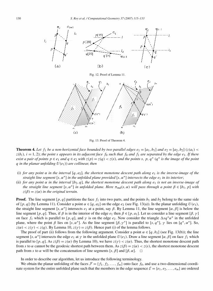
Consider a horizontal plane h at altitude z(p). The intersection of the face f and the plane h is the line segment[p,q] (by part (i) of this lemma). Consider another horizontal plane h′ through a point r on line �. The intersectionof f and h′ must be parallel to [p,q], and hence it coincides with the line �. Thus, all the points on the line � have thesame z-coordinate. �Lemma 11. Let ei and ei+1 be two edges in E bounding a face f . For a pair of points p,p′ ∈ ei and a pair of pointsq, q ′ ∈ ei+1, if z(p) > z(p′) and z(q) > z(q ′), then the line segments [p,q] and [p′, q ′] does not intersect in face f ;but the line segments [p,q ′] and [p′, q] must intersect in face f .

Proof. Without loss of generality, assume that z(p) > z(q). Draw two horizontal planes h1 and h2 through p and q

respectively which intersect face f along the lines �1 and �2 respectively. Note that �1 is above �2 with respect totheir z-coordinates. Here any one of the three cases may arise: (i) both p′ and q ′ are above h2, (ii) both p′ and q ′ arebelow h2, (iii) p′ and q ′ appear in different sides of h2. Case (i) is impossible since z(q) > z(q ′). In Case (ii), the linesegment [p,q] and [p′, q ′] appear in different sides of the plane h2, and hence they cannot intersect (see Fig. 12(a)).In Case (iii), z(p′) > z(q) and z(q ′) < z(q). Here, if [p,q] and [p′, q ′] intersects, then ei and ei+1 cannot be parallel(see Fig. 12(b)). The reason is that, as ei and ei+1 are parallel and z(p) > z(p′) > z(q) & z(q) > z(q ′), then [p,q]and [p′, q ′] are the sides (not the diagonals) of the trapezoid �pp′q ′q (see Fig. 12(c)). �

130 S. Roy et al. / Computational Geometry 37 (2007) 115–133

Fig. 12. Proof of Lemma 11.

Fig. 13. Proof of Theorem 4.

Theorem 4. Let f1 be a non-horizontal face bounded by two parallel edges e1 = [a1, b1] and e2 = [a2, b2] (z(ai) <

z(bi), i = 1,2); the point s appears in its adjacent face f0 such that f0 and f1 are separated by the edge e1. If thereexist a pair of points p ∈ e1 and q ∈ e2 with z(p) = z(q) < z(s), and the points s, p, q∗ (q∗ is the image of the pointq in the planar unfolding U(e1)) are collinear, then

(i) for any point α in the interval [q, a2], the shortest monotone descent path along e1 is the inverse-image of thestraight line segment [s,α∗] in the unfolded plane provided [s,α∗] intersects the edge e1 in its interior;

(ii) for any point α in the interval [b2, q], the shortest monotone descent path along e1 is not an inverse-image ofthe straight line segment [s,α∗] in unfolded plane. Here πmd(s,α) will pass through a point β ∈ [b1,p] withz(β) = z(α) in the original terrain.

Proof. The line segment [p,q] partitions the face f1 into two parts, and the points b1 and b2 belong to the same sideof [p,q] (by Lemma 11). Consider a point α ∈ [q, a2] on the edge e2 (see Fig. 13(a)). In the planar unfolding U(e1),the straight line segment [s,α∗] intersects e1 at a point, say β . By Lemma 11, the line segment [α,β] is below theline segment [p,q]. Thus, if β is in the interior of the edge e1 then β ∈ [p,a1]. Let us consider a line segment [β,γ ]on face f1 which is parallel to [p,q], and γ is on the edge e2. Now consider the triangle sq∗α∗ in the unfoldedplane, where the point β lies on [s,α∗]. As the line segment [β,γ ∗] is parallel to [s, q∗], γ lies on [q∗, α∗]. So,z(α) < z(γ ) < z(q). By Lemma 10, z(γ ) = z(β). Hence part (i) of the lemma follows.

The proof of part (ii) follows from the following argument. Consider a point α ∈ [q, b2] (see Fig. 13(b)); the linesegment [s,α∗] intersects the edge e1 at γ in the unfolded plane U(e1). Draw a line segment [α,β] on face f1 whichis parallel to [p,q]. As z(β) = z(α) (by Lemma 10), we have z(γ ) < z(α). Thus, the shortest monotone descent pathfrom s to α cannot be the geodesic shortest path between them. As z(β) = z(α) < z(s), the shortest monotone descentpath from s to α will be the concatenation of line segments [s, β] and [β,α]. �

In order to describe our algorithm, let us introduce the following terminology.We obtain the planar unfolding of the faces F = {f1, f2, . . . , fm} onto face f0, and use a two-dimensional coordi-

nate system for the entire unfolded plane such that the members in the edge sequence E = {e1, e2, . . . , em} are ordered

S. Roy et al. / Computational Geometry 37 (2007) 115–133 131

from left to right, and each of them is parallel to the y-axis. The z-coordinate of a point in the unfolded plane indicatesthe z-coordinate of that point in the original terrain. In this planar unfolding, if an edge ei of the terrain is representedas [ai, bi], with y(ai) < y(bi) then z(ai) � z(bi) (see Lemma 10). The source s is in f0, then flow passes throughthe edge sequence E to reach a point t ∈ fm. If a path π(s, t) enters into a face fi along a line �i , then the angle ofincidence of π(s, t) in face fi (with edge ei ) is denoted by θi , and henceforth will be referred to as slope of �i .

Let e1 and e2 be two parallel boundaries of a face f . The translation event for face f , denoted by T (f ) is a lineartranslation of e2 on e1 such that the entire face f is merged to the line e1 as follows:

The points in the unfolded plane lying on the same side of s with respect to e1 remain unchanged.

Each point p lying in the proper interior of the face f is mapped to a point q ∈ e1 such that z(p) = z(q).

Each point p = (x(p), y(p)) on the edge e2 is mapped to a point q = (x(q), y(q)) on the edge e1 such thatz(p) = z(q). Under this transformation x(q) = x(p) + α, y(q) = y(p) + β , where the tuple (α,β) are constant,and they depend on the slope and width of the face f .

Each point (x, y) in the unfolded plane lying on the other side of s with respect to e2 is moved to the point(x + α,y + β).

The slope of the line containing [p,q] is referred to as merging direction of face f , and is denoted as φ(f ). Theorem 4indicates the following result.

Corollary 4.1. If the slope θ of a line segment � in face f is such that (i) θ < φ(f ) then � is strictly monotone descent,(ii) θ = φ(f ) then all the points in � have same z-coordinate, and (iii) θ > φ(f ) then � is strictly monotone ascent.

Let πmd(s, t) be the shortest monotone descent path from s ∈ f0 to t ∈ fm passing through a sequence of paralleledges {e1, e2, . . . , em−1}. Along this path there exists a set of faces {fji

, i = 1,2, . . . , k} such that all the points of thepath πmd(s, t) in face fji

have same z-coordinate ξji; the portions of the path in all other faces are strictly monotone

descent. Now, we have the following theorem.

Theorem 5. If the translations T (fj1), T (fj2), . . . , T (fjk) are applied (in any order) on the unfolded plane of faces

f0, f1, . . . , fm then the shortest monotone descent path πmd(s, t) will become a straight line segment from s to t inthe transformed plane.

Proof. Let us first assume that k = 1, i.e., πmd(s, t) passes through a face f with all points having the same z-coordinate. Let fa and fb be its preceding and succeeding faces with separating edges ea and eb respectively. Wealso assume that πmd(s, t) consists of three consecutive line segments [s, a], [a, b], [b, t] lying in fa , f and fb

respectively. Note that all the points on [a, b] have same z-coordinate. If we apply T (f ), the points b and t will bemapped to a and t ′. Now, in the transformed plane, the shortest path from s to t ′ is the straight line segment [s, t ′].We argue that [s, t ′] will pass through a. On the contrary, assume that [s, t ′] intersect ea at a′, and a′ is the imageof b′ ∈ eb under T (f ), b′ = b. Thus, d(s, a′) + d(a′, t ′) < d(s, a) + d(a, t ′). Now, applying reverse transformation,d(s, a′) + d(b′, t) < d(s, a) + d(b, t). From Lemma 10, d(s, a′) + d(a′, b′) + d(b′, t) < d(s, a) + d(a, b) + d(b, t).This leads to a contradiction.

Let there exist several faces on the path πmd(s, t) such that all the points of πmd(s, t) in that face have same z-coordinate. If we apply the transformation T on one face at a time, the above result holds. The order of choosing theface for applying the transformation T is not important due to the following argument: (i) a point p on the unfoldedplane will be affected due to same set of transformation irrespective of in which order they are applied, and (ii) theeffects of all the transformations affecting on a point are additive. �Lemma 12. If the shortest monotone descent path πmd(s, t) is passing through a sequence of parallel edges, then allthe line segments of πmd(s, t), which are strictly monotone descent, are parallel on the unfolded plane of all faces.

132 S. Roy et al. / Computational Geometry 37 (2007) 115–133

Theorem 6. If the line segments of shortest monotone descent path πmd(s, t) in faces f1∗ , f2∗ , . . . , fk∗ are strictlymonotone then their slopes are equal. The slope of the portions of πmd(s, t) in all other faces are equal to the mergingangle of the corresponding faces.

The above discussions lead to the following algorithm for computing the shortest monotone descent path betweena pair of points s (source) and t (destination) through a sequence of faces separated by mutually parallel edges.

5.2. Algorithm

Step 1. We compute the planar unfolding where the faces f1, f2, . . . , fm are unfolded onto face f0 containing s. Weassume that the entire terrain is in first quadrant, and all the edges of T are parallel to the y-axis.

Step 2. We compute the merging angle for all the faces fi, i = 1,2, . . . ,m, and store them in an array Φ in ascendingorder. Each element contains its face-id.

Step 3. (*Merging phase*) Let θ be the slope of the line joining s and t in the unfolded plane. We sequentially inspectthe elements of the array Φ from its first element onwards until an element Φ[k] > θ is obtained. For each elementΦ[i], i < k, the translation event takes place, and we do the following:

Let Φ[i] correspond to a face f . We transform the entire terrain by merging the two boundaries of face f , i.e.,compute the destination point t under the translation. The face f is marked. We update θ by joining s with the newposition of t .

Compute the optimum path in transformed plane by the line joining s and t .

Step 4. After the execution of Step 3, the value of θ indicates the slope of the path segments which are strictlymonotone descent along πmd(s, t). We compute πmd(s, t) as follows:

Start from the point s at face f0, and consider each face fi, i = 1,2, . . . ,m in order. If face fi is not marked,πmd(s, t) moves in that face along a line segment of slope θ ; otherwise, πmd(s, t) moves along a line segment ofslope Φ[i].

Step 5. Finally, report the optimum path πmd(s, t).

5.3. Correctness and complexity analysis of the algorithm

Theorem 7. Our algorithm correctly computes the shortest monotone descent path between two query points s and t

through a sequence of faces of a polyhedral terrain bounded by parallel edges in O(m logm) time.

Proof. We prove the correctness of the algorithm by contradiction. The path obtained by our algorithm is π(s, t).It passes through the faces at equal altitude for which the merging angles are {Φ[1], . . . ,Φ[k]} (⊆ Φ), and followsstrictly monotone descent (with angle = θ ) in the faces having merging angles {Φ[k +1],Φ[k +2], . . . ,Φ[m]}, whereΦ[i] < θ for i = 1, . . . , k, and Φ[i] > θ for i = k + 1, . . . ,m.

Let the optimum path π ′(s, t) passes through the faces at equal altitude for which the merging angles are{Φ[1], . . . ,Φ[k′]} (⊆ Φ), and follows strictly monotone descent (with angle = θ ′) in the faces having merging angles{Φ[k′ + 1],Φ[k′ + 2], . . . ,Φ[m]}, where Φ[i] < θ ′ for i = 1, . . . , k′, and Φ[i] > θ ′ for i = k′ + 1, . . . ,m.

If k = k′, then θ = θ ′ (by Theorems 5 and 6), and the path obtained by our algorithm is optimum.Let us assume that k < k′, or in other words, θ < θ ′ (since Φ is created in ascending order of merging angles).

Thus, our algorithm chooses few more faces than the optimum solution where the path goes through the same height.Now, the three cases stated below are exhaustive.

As θ < θ ′, π ′(s, t) will diverge upwards from π(s, t) in all the faces where both the paths follow strictly monotonedescent property.

S. Roy et al. / Computational Geometry 37 (2007) 115–133 133

In some faces π ′(s, t) goes through equal height but π(s, t) follows monotone descent property. There also π ′(s, t)will diverge upwards from π(s, t).

In those faces where π ′(s, t) and π(s, t) goes through equal height, they remain parallel.

Since π(s, t) has reached t , π ′(s, t) will reach somewhere above t in face fm. The similar argument proves that k > k′.Given a sequence of m faces of a polyhedral terrain bounded by parallel lines, and two query points s and t , Steps 1

and 2 of the algorithm computes the merging angles and sorts them in O(m logm) time. Step 3 needs O(1) time. Eachiteration of Step 4 needs O(1) time, and we may need O(n) such iterations for reporting the shortest monotone descentpath from s and t . Thus the time complexity result follows. �6. Conclusion

We have proposed polynomial time algorithms for finding the shortest monotone descent path from a point s to apoint t in a polyhedral terrains in two special cases where (i) t is a point in convex DFR(s), and (ii) the path from s tot passes through a set of faces bounded by parallel edges. The same problem for the general terrain is still unsolved.

Acknowledgements

We sincerely acknowledge the two anonymous referees of this paper. Their suggestions helped us enormously toimprove the quality of the paper.

References

[1] P.K. Agarwal, S. Har-Peled, M. Karia, Computing approximate shortest paths on convex polytopes, Algorithmica 33 (2002) 227–242.[2] L. Aleksandrov, A. Maheshwari, J.-R. Sack, Approximation algorithms for geometric shortest path problems, in: Proc. Symp. on Theory of

Comput., 2000, pp. 286–295.[3] L. Aleksandrov, A. Maheshwari, J.-R. Sack, An improved approximation algorithms for computing geometric shortest paths problems, in:

Proc. Symp. on Foundations of Computing Theory, 2003, pp. 246–257.[4] L. Aleksandrov, A. Maheshwari, J.-R. Sack, Determining approximate shortest paths on weighted polyhedral surfaces, J. ACM 52 (2005)

25–53.[5] M. de Berg, M. van Kreveld, Trekking in the Alps without freezing or getting tired, Algorithmica 18 (1997) 306–323.[6] J. Chen, Y. Han, Shortest paths on a polyhedron, Internat. J. Comput. Geom. Appl. 6 (1996) 127–144.[7] S. Fortune, A sweepline algorithm for Voronoi diagrams, Algorithmica 2 (1987) 153–174.[8] S. Kapoor, Efficient computation of geodesic shortest paths, in: Symp. on Theory of Computing, 1999, pp. 770–779.[9] J. Hershberger, S. Suri, Practical methods for approximating shortest paths on a convex polytopes in R3, Comput. Geom. Theory Appl. 10

(1998) 31–46.[10] D.G. Kirkpatrick, Optimal search in planar subdivisions, SIAM J. Comput. 12 (1983) 28–35.[11] M. Lanthier, A. Maheswari, J.-R. Sack, Approximating weighted shortest paths on polyhedral surfaces, Algorithmica 30 (2001) 527–562.[12] C. Mata, J.S.B. Mitchell, A new algorithm for computing shortest paths in weighted planar subdivisions, in: Proc. 13th ACM Symp. Comput.

Geom., 1997, pp. 264–273.[13] J.S.B. Mitchell, D.M. Mount, C.H. Papadimitrou, The discrete geodesic problem, SIAM J. Comput. 16 (1987) 647–668.[14] J.S.B. Mitchell, C.H. Papadimitrou, The weighted region problem: Finding shortest paths through a weighted planar subdivision, J. Assoc.

Comput. Mach. 38 (1991) 18–73.[15] J.S.B. Mitchell, M. Sharir, New results on shortest paths in three dimensions, in: Proc. of the Twentieth Symposium on Computational

Geometry, 2004, pp. 124–133.[16] J.H. Reif, Z. Sun, An efficient approximation algorithm for weighted region shortest path problem, in: Proc. of the Workshop on Algorithmic

Foundations of Robotics, 2000, pp. 191–203.[17] S. Roy, S. Das, S.C. Nandy, A practical algorithm for approximating shortest weighted path between a pair of points on polyhedral surface,

in: Int. Conf. on Computational Science and Its Applications, 2004, pp. 42–52.[18] J.R. Sack, J. Urrutia, Handbook of Computational Geometry, North-Holland/Elsevier, Netherlands, 2000.[19] M. Sharir, A. Schorr, On shortest paths in polyhedral space, SIAM J. Comput. 15 (1986) 193–215.[20] K.R. Varadarajan, P.K. Agarwal, Approximating shortest paths on a non-convex polyhedron, SIAM J. Comput. 30 (2001) 1321–1340.