Uniform controllability of semidiscrete approximations of parabolic control systems

YOUNG-MEASURE APPROXIMATIONS FOR
ELASTODYNAMICS WITH NON-MONOTONE
STRESS-STRAIN RELATIONS
C. CARSTENSEN AND M. O. RIEGER
Abstract. Microstructures in phase-transitions of alloys are mod-
eled by the energy minimization of a nonconvex energy density
φ. Their time-evolution leads to a nonlinear wave equation utt =
div S(Du) with the non-monotone stress-strain relation S = Dφ
plus proper boundary and initial conditions. This hyperbolic-
elliptic initial-boundary value problem of changing types allows,
in general, solely Young measure solutions. This paper introduces
a fully-numerical time-space discretization of this equation in a
corresponding very weak sense. It is shown that discrete solutions
exist and generate weakly convergent subsequences whose limit
is a Young measure solution. Numerical examples in one space
dimension illustrate the time-evolving phase transitions and mi-
crostructures of a nonlinearly vibrating string.
1. Introduction
The numerical simulation of a nonlinear wave equation
(1.1) utt = div S(Du) in Q = Ω × (0, T ),
the space-time domain, plus boundary and initial conditions is cer-
tainly one of the more important tasks in computational sciences and
engineering. The hyperbolic nature of (1.1) possibly leads to disconti-
nuities (e.g. shocks). The nonlinear stress-strain relation S = Dφ is
modeled by the gradient of a smooth function φ. Even for convex φ it
is, in general, unknown whether or not there always exist weak solu-
tions in the class of Sobolev functions. There are, however, affirmative
results if Ω ⊂ R is one-dimensional, in particular the seminal works by
DiPerna, Murat and Tartar where Young-measures had been used to
obtain global existence results (see, e.g., [Tay96] for further references).
In higher dimensions there are local results for small T > 0 [DH85].
1991 Mathematics Subject Classification. 65P25, 35G25, 47J35.Key words and phrases. Non-Monotone Evolution, Nonlinear Elastodynamics,
Young Measure Approximation, Nonlinear Wave Equation.1

2 C. CARSTENSEN AND M. O. RIEGER
The simulation of phase-transition problems motivates nonconvex
energy densities φ where weak solutions may not exist. Instead, oscil-
lations are likely to occur which can be described mathematically using
the concept of Young-measure valued solutions (see Section 2). The
following example suggests that even if classical solutions are present,
there may exist further Young-measure solutions with more physical
relevance.
Example. Let Ω = (0, 1) denote the unit interval and let φ(y) =
(1 − y2)2 denote the 2-well energy density. Given a parameter λ ∈ R,
the initial conditions u0(x) = λ x and u1(x) = 0 for 0 < x < 1 and
the boundary conditions u(x, ·) = λ x for x = 0 and x = 1 we obtain
the classical stationary solution u(·, t) = u0(·). For −1 < λ < 1 and
µ := (1 − λ)/2, the measure ν := µδ−1 + (1 − µ)δ+1 defines a Young-
measure solution in the sense specified below in this paper. Here and
below, δ±1 denotes the Dirac measure supported at ±1, the two wells
where the energy density φ is minimal.
In contrast to the smooth classical solution u0, the measure valued
solution defined by ν does describe oscillations in agreement to observa-
tions in physical experiments. Moreover, the total energy of the Young
measure solution is zero, whereas the classical solution has the energy
φ(λ) > 0. Finally, for |λ| < 3−1/2, the classical solution is instable, a
linearized model leads to an oscilator with a spring of negative stiffness
φ′′(λ). However, the Young measure solution is stable, in the sense that
it corresponds to a state with minimal energy.
In conclusion, the Young measure solution is a very relevant object;
its numerical simulation appears an innovative task and is therefore
introduced in this paper.
For the numerical simulation with (1.1), a viscous regularization
(1.2) utt = div S(Du) + µ∆ut
has been proposed [KL94, CD03] for a small parameter µ > 0, the vis-
cosity. It is known that the initial-boundary value problem with (1.2)
has a solution if S is, e.g., globally Lipschitz continuous, but possibly
non-monotone [FD97]. Moreover, the numerical analysis of a backward
time-step discretization combined with a finite element discretization
of Ω in space was reported in [KL94] to be instable for µ > 0 and
a nonconforming FEM was suggested. Recently, the convergence for
the conforming FEM was established under strong regularity assump-
tions of the unique exact solution in [CD03]. The situation for µ = 0,
however, cannot be handled since some a priori bounds of the discrete

SIMULATIONS IN NON-MONOTONE ELASTODYNAMICS 3
FE solutions are missing in the passage to the limit. As a consequence,
measure-valued solution concepts are necessary which are weak enough
to allow high oscillations in the limit. In particular the notion of Young
measures as they were originally introduced by L.C. Young under the
name “generalized curves” (see [You37, You69]) turned out to be an
adequate concept in the 1970s with the work of L. Tartar (see [Tar79]
and [BL73, BJ87] for stimulating contributions).
The numerical simulation of related nonconvex minimization prob-
lems has been studied in [CCK95, CKL91, CL91, Lus96] for a di-
rect minimization, in [CP97, Car01] for a convexified situation, and
in [NW93, Rou97, CR00, Car01] for a measure-valued generalization.
Time-evolution problems have been studied analytically in [Sle91, KP92,
Dem96, Dem97, Rie00, Rie03, RZ02] and are numerically addressed in
this paper in the spirit of [CR00].
The remaining part of the paper is organized as follows. Section 2
establishes the concept of Young-measure solutions of (1.1) and states
an existence result in Theorem 2.1. The consistent discretization in
space-time is addressed in Section 3 where we introduce a numerical
scheme, prove existence of discrete solutions, a discrete energy estimate,
and a convergence result. The numerical realization is explained in
Section 4 before several numerical simulations are reported in Section 5.
Some extending remarks conclude the paper with Section 6.
We will use the following notations: Throughout this article, Ω de-
notes an open domain in Rn with Lipschitz boundary. Lp(Ω) denotes
the Lebesgue space of functions u such that |u|p is integrable; L∞(Ω) the
space of bounded functions; W m,p(A, B) is the Sobolev space of all func-
tions u : A → B with Dmu in Lp(Ω) for p ∈ [1,∞], where Dm denotes
partial derivatives of order m ∈ N. We write Hm(A, B) := W m,2(A, B).
Let p < ∞. A sequence of functions un is said to be weakly converging
to a limit function u in Lp(Ω) if un ∈ Lp(Ω) and for all test functions
ζ ∈ Lp′ with 1/p + 1/p′ = 1 we have∫
Ω
unζ →∫
Ω
uζ.
We denote this by un u in Lp(Ω). Similarly we say that un u in
W m,p(Ω) if un ∈ W m,p(Ω) and for all ζ ∈ W m,p′(Ω)∫
Ω
unDmζ →
∫
Ω
uDmζ.

4 C. CARSTENSEN AND M. O. RIEGER
A function f : Rm×n → R is called quasiconvex if it satisfies
∫
Ω
f(P + Dφ) dx ≥ |Ω| f(P )
for every test function φ (i.e. φ ∈ C∞(Ω) with supp φ compactly in Ω)
and every P ∈ Rm×n.
Finally by φ∗∗ we denote the convexification of φ (the largest convex
function below φ) and by φqc the quasiconvexification of φ (the largest
quasiconvex function below φ).
2. Young-Measure-Valued Solutions
The aim of this section is to establish a time discretization scheme
for nonconvex elastodynamical equations converging to a Young mea-
sure solution. The statistics of the oscillating deformation gradient of
our approximate solution is described by a probability measure. The
constructive existence proof in Section 3 is the basis for the numerical
simulations below.
Given initial data u0 ∈ H10 (Ω; Rn), v0 ∈ L2(Ω; Rn), and boundary
data g ∈ H1(Ω), the nonlinear system of elastic time evolution reads
utt = div S(Du) (in the sense of distributions),(2.1)
u(x, 0) = u0(x) for almost every x ∈ Ω,(2.2)
ut(x, 0) = v0(x) for almost every x ∈ Ω,(2.3)
u(x, 0) = g(x) for x ∈ ∂Ω (in the sense of traces).(2.4)
The non-negative energy density φ ∈ C1(Rm×n) and its derivative S :=
Dφ : Rm×n → R
m×n satisfy for some constants α, β > 0 certain growth
conditions formulated with the spaces E0 and F0.
By E0 we denote the space of continuous functions with specified
quadratic growth and by F0 the space with linear growth,
E0 =
f ∈ C(Rm×n; R+)
∣∣∣∣∣ lim||A||→∞
f(A)
1 + ||A||2 exists and is finite
,
F0 =
f ∈ C(Rm×n; R+)
∣∣∣∣∣ lim||A||→∞
f(A)
1 + ||A|| exists and is finite
.
The vector spaces E0 and F0 are endowed with the norms
‖f‖E0:= sup
A
|f(A)|1 + ||A||2 and ‖f‖F0
:= supA
|f(A)|1 + ||A|| ,
respectively.

SIMULATIONS IN NON-MONOTONE ELASTODYNAMICS 5
A probability measure ν is a non-negative Radon measure on a set E
with ν(E) = 1. A Young measure (or parameterized measure) is a fam-
ily of probability measures (νx)x∈Ω on RN associated with a sequence
of measurable functions (fj)j∈N with fj : Ω ⊂ Rn → R
N such that for
any continuous function φ : RN → R the function
φ(x) =
∫
RN
φ(F ) dνx(F ) =: 〈νx, φ〉
is measurable, and for every weakly-converging sequence (fj) we have
for all open subsets Ω0 ⊂ Ω∫
Ω0
(φ(fj))j(x) dx →∫
Ω0
φ(x) dx.
We can think of the Young measure as a “one-point statistic” for
the sequence fj , i.e. νx describes (in a certain sense which can be made
mathematically precise [Ped97]) the probability distribution of the val-
ues of the sequence fj near x ∈ Ω. For an introduction into Young
measures and their applications see [Ped97, Mul99].
Theorem 2.1 (Existence of Young measure solution). Given φ ∈ E0
with S := Dφ ∈ F0, such that φqc is convex and φ(A) ≥ α(||A||2 − 1),
u0 ∈ H1(Ω), u1 ∈ H1(Ω), g ∈ H1(Ω) and Q := Ω × (0, T ) ⊂ Rn+1,
there exists a Young measure solution (u, ν) of (2.1)-(2.4) in the sense
that
u − g ∈ W 1,∞((0, T ); L2(Ω)) ∩ L∞((0, T ); W 1,20 (Ω)),
u(x, 0) = u0(x), ut(x, 0) = u1(x) for all x ∈ Ω,
ν = (νx,t : (x, t) ∈ Q) is a family of probability measure,∫ T
0
∫Ω(〈ν, S〉∇ζ − utζt) dx dt = 0 for all ζ ∈ C∞
0 (Q),
Du(x, t) = 〈νx,t, Id〉 for almost every (x, t) ∈ Q.
Here 〈ν, S〉 is defined as dual pairing of S with the measure ν, i.e.
〈ν, S〉 :=
∫
Rm×n
S(A) dν(A).
Remark 2.2. If the Young measure ν is a Dirac measure for almost
every (x, t) ∈ Q, then u is a weak solution of the elastodynamical system
(2.1)-(2.4).
Remark 2.3. For φ ∈ E0, S ∈ F0 and A ∈ Rm×n there holds
φ(A) ≤ β(||A||2 + 1),(2.5)
|S(A)| ≤ β(||A||+ 1).(2.6)
6 C. CARSTENSEN AND M. O. RIEGER
Remark 2.4. The condition that φqc is convex is automatically satisfied
for n = 1 or m = 1. The condition is needed to establish an a priori
energy estimate for the solutions of the time discretized problem. If such
bounds exist, the condition is not necessary in the proof of Theorem 2.1.
Remark 2.5. Alternative approximation schemes which can ensure
existence in the case where φqc is nonconvex will be discussed Section 6.
3. Numerical Schemes and Constructive Existence Proof
The proof of Theorem 2.1 is based on a discretization in time, energy
estimates, and relaxation for each time-step [Dem97, Rie00]. The limit
for infinitely small time steps then provides the asserted regularity of
the solution. Without loss of generality let g ≡ 0 (as a shift of u to u−g
would result in a problem with homogeneous boundary conditions).
3.1. Time Discretization.
Definition 3.1. Given u0, v0, g ≡ 0, and h > 0 with an integer N =
T/h, find (uh,j)h,j such that uh,0 = u0, uh,−1 = u0 − hv0, and uhj ∈H1
0 (Ω; Rm) satisfies, for j = 1, 2 . . . , N ,
(3.1)uh,j − 2uh,j−1 + uh,j−2
h2− div S(Duh,j) = 0.
In the following we abbreviate
(3.2) vh,j :=uh,j − uh,j−1
hand
(3.3) Ej := Eh,j :=
∫
Ω
(φqc(Duh,j) +
1
2|vh,j|2
).
Theorem 3.2 (Discrete Solution). The relaxed time-discretized system
(3.4)
∫
Ω
(⟨νh,j, S
⟩Dζ +
uh,j − 2uh,j−1 + uh,j−2
h2ζ
)dx = 0
with j ∈ N and ζ ∈ H10 (Ω; Rm) admits a solution (uh,j, νh,j) where
uh,j ∈ H10 (Ω; Rm) and νh,j is a Young measure with 〈νh,j, Id〉 = Duh,j.
Proof. The discrete problem (3.1) reads as a minimization problem for
the energy functional
Wj(v) := W (v; uh,j−1, uh,j−2)
:=
∫
Ω
(φ(Dv) +
|v − 2uh,j−1 + uh,j−2|22h2
).
Any minimizer u of Wj is a solution of the discretized differential equa-
tions. But, in general, Wj is not weakly lower semicontinuous (w.l.s.c.)

SIMULATIONS IN NON-MONOTONE ELASTODYNAMICS 7
since φ is not assumed to be quasiconvex. Hence the existence of a
minimizing Sobolev function u cannot be expected. To describe more
general solution concepts we consider W qcj , the quasiconvexification of
the energy function Wj, i.e.
W qcj (v) :=
∫
Ω
(φqc(Dv) +
|v − 2uh,j−1 + uh,j−2|22h2
).
Since W qcj is w.l.s.c. there exists a minimizer uh,j with
infj
Wj(v) = infv
W qcj (v) = W qc
j (uh,j).
Then, one can prove the theorem by relaxation theory as in [Dem97].
2
3.2. Space Discretization. For each time-step, a Galerkin discretiza-
tion is needed for the time-discretized system (3.4). A uniform partition
with mesh-size dx = L/M in M subintervals I1, I2, . . . , IM of Ω = (0, L)
defines the first-order finite element spaces
Sh := vh ∈ C(Ω)| ∀k = 1, 2, . . . , M, vh affine on Ik,Hh,g := vh ∈ Sh| vh = g on ∂Ω, and Hh,0 := Sh ∩ H1
0 (Ω).
On each interval Ik := ((k − 1)dx, k dx), the Young measure νh,j is
discretized as a finite sum of q Dirac measures. The chosen supports
F1, . . . , Fq discretize R and each discrete Young measure assumes the
representation
(3.5) νh,j |Ik=
q∑
`=1
λj,k,`δF`on Ik, k = 1, . . . , M,
with unknown convex coefficients
(3.6) λj,k,1, . . . , λj,k,q ≥ 0 with
q∑
`=1
λj,k,` = 1
and subject to the side-restriction
(3.7)
q∑
`=1
λj,k,`F` = ∂uh,j/∂x |Ik.
Then define
Y Mh := νh,j Young measure| νh,j satisfies (3.5) for coefficients
with (3.6),Bj := (uh,j
h , νh,j) ∈ Hh,g × Y Mh| uh,j and νh,j satisfies (3.7).

8 C. CARSTENSEN AND M. O. RIEGER
Definition 3.3 (Fully discrete Problem). Given u0, v0, g, h > 0, dx >
0 such that N = T/h and M = L/dx are integers, set uh,0 = u0,
uh,−1 = u0 − hv0 at the nodes xk = k dx for k = 0, 1, . . . , M and for all
j = 1, . . . , N , find (uh,j, νh,j) ∈ Bj which satisfies∫
Ω
(⟨νh,j, S
⟩vh + h−2(uh,j − 2uh,j−1 + uh,j−2)vh
)dx = 0
for all test functions vh ∈ Hh,0.
Theorem 3.4. The fully discrete problem has a unique solution uh,j.
Proof. The proof is based on the stationary situation within each time-
step essentially given in [CR00, Rou97]. The uniqueness of the discrete
displacement variables results from the uniform monotonicity of the
low-order time-difference term. 2
Remark 3.5. The uniqueness of the discrete Young measures is related
to the 2-well problem which defines the convex hull uniquely. In the
discrete situation, however, it may be that the minimizing Young mea-
sure is non-unique. For instance, let F1, F2, F3 and F4 denote the four
distinct real arguments with φ(Fn) = 0.1 in the situation for φ of Fig-
ure 3.1. Then, even though the mean u′h|Ij
= νh,j = λ1F1+· · ·+λ4F4 =
0 is unique, there are infinitely many convex coefficients λ1, . . . , λ4 ≥ 0
with λ1F1+· · ·+λ4F4 = 0 and λ1+· · ·+λ4 = 1. Each of those solutions
defines a different Young measure which may be part of one different
solution of the fully discrete problem.
Remark 3.6. The effective numerical solution is performed with a mul-
tilevel active-set strategy of [CR00] based on the Weierstrass maximum
principle for Lagrange multipliers. The practical performance shows
linear complexity in the number of unknowns [CR00].
Remark 3.7. Weak convergence as dx → 0 and q → ∞ follows with
the direct method of the calculus of variations, cf. [Rou97] for details.
Strong convergence is less obvious. We refer to [CP97] for a related
problem (obtained for q = ∞ by convexification).
3.3. Discrete Energy Estimate. In order to prove the convergence
of the discrete solution to a solution of the original problem it is neces-
sary to obtain some a priori energy estimates for the discrete solutions
which are independent of the discretization parameter h > 0. We can
prove the following result:
Theorem 3.8 (Discrete Energy Estimate). Suppose φqc is convex, that
α is as in Theorem 2.1, and that uh,j, vh,j solve (3.1)-(3.3) for all j =

SIMULATIONS IN NON-MONOTONE ELASTODYNAMICS 9
1, . . . , N . Then, for all j = 1, . . . , N ,
(3.8) ||uh,j||2H1 + ||vh,j||2 ≤ 1
α(2E0 + |Ω|) and Ej ≤ E0 < ∞.
Proof. Proposition 3.6 in [BKK00] reads Dφqc(∇uh,j) =⟨νh,j, S
⟩. Mul-
tiplication of the discrete elasticity equation with vh,j, integration in
space and summing over all j leads to
∫
Ω
∑
j
vh,j − vh,j−1
hvh,j dx = −
∫
Ω
∑
j
Dφqc(∇uh,j)∇vh,j
hdx.
Since φqc is convex by assumption one can use Jensen’s inequality to
obtain from this the discrete energy inequality (3.8).
3.4. Weak convergence of the time discretization.
Theorem 3.9. The solutions uh,j, vh,j of the time discretized problem
are convergent as h → 0 if and only if they satisfy the a priori estimate
(3.8).
For the proof considers the piecewise constant and piecewise affine
interpolations of the nodal values (uh,j), (vh,j), (vh,j − vh,j−1)/h and
(νh,j). The separability of F0 and E0 is used to obtain a weakly con-
verging subsequence for the Young measures (νh,j). The discrete energy
inequality yields bounds for the other interpolations. The technicali-
ties follow arguments of [Dem96] (in a slightly different notation) and
hence are suppressed in the sequel.
For h > 0, j ∈ N, and the characteristic function χh,j := χ[hj,h(j+1)]
of the set [hj, h(j +1)] for jh < t < h(j +1), where χA(x) := 1 if x ∈ A
and χA(x) = 0 elsewhere.
wh(t) :=∑
j
χh,j(t)vh,j+1 − vh,j
h
(step function approximation of utt),
vh(t) :=∑
j
χh,j(t)
(vh,j +
vh,j+1 − vh,j
h(t − hj)
)
(the primitive of wh),

10 C. CARSTENSEN AND M. O. RIEGER
vh(t) :=∑
j
χh,j(t)vh,j+1 (step function approximation of ut),
uh(t) :=∑
j
χh,j(t)(uh,j + vh,j+1(t − hj)
)(its primitive),
uh(t) :=∑
j
χh,j(t)uh,j+1 (step function approximation of u),
νh := (νhx,t)(x,t) :=
∑
j
χh,j(t)νh,j+1x (Young measure).
One can prove that the Young measure νh is generated by the se-
quence(∑
j χh,j(t)Duh,j,k)
k. Moreover there holds
νh ∈ L1loc(Ω × (0, T0); E ′
0) ∩ L2loc(Ω × (0, T0),F ′
0).
With νh and wh one can recast (3.1) for t ≥ h and ζ ∈ H10 (Ω; Rm)
into
(3.9)
∫
Ω
(⟨νh
x,t, S⟩Dζ + wh(x, t)ζ
)dx = 0.
An integration over (h, T0) leads to
(3.10)∫ T0
h
∫
Ω
(⟨νh
x,t, S⟩Dζ − vh(x, t)ζt(x)
)dx dt = 0. for all ζ ∈ H1
0
Then one proves Duh =⟨νh, Id
⟩. A short calculation shows
(3.11) uh(·, 0) = u0, and vht (·, 0) = v0.
The aim is to prove that uh and νh converge in an appropriate norm to
a solution of the original problem. One observes that (νh)h is bounded
in L2loc(Ω × R
+;F ′0). Since F0 is separable,
L2loc(Ω × R
+;F ′0)
∼=(L2
loc(Ω × R+;F0)
)′.
Hence the bounded sequence (νh)h has a subsequence (not relabeled)
which converges weakly in (L2loc(Ω × R
+;F0))′. Therefore for all g ∈
L2loc(Ω × R
+;F0),
(∫ T0
0
∫
Ω
〈νhx,t, gx,t〉 dx dt
)h→
∫ T0
0
∫
Ω
〈νx,t, gx,t〉dx dt.
For test functions gx,t(y) = f(y)ζ(x, t) with ζ ∈ L2loc(Ω × R
+) and
f ∈ F0, this yields
(3.12) (〈νh, f〉)h 〈ν, f〉 in L2loc(Ω × R
+).
The same arguments show
(3.13) (νh)h ν in L2loc(Ω × R
+;F ′0) ∩ L1
loc(Ω × R+; E ′
0).

SIMULATIONS IN NON-MONOTONE ELASTODYNAMICS 11
Moreover, there exists a diagonal sequence of(∑
j χh,j(t)uh,j,k)
h,kwhich
generates the Young measure ν. Since Dφ, Dφqc ∈ F0 leads to
(〈νh, Dφ〉)h 〈ν, Dφ〉,(〈νh, Dφqc〉)h 〈ν, Dφqc〉 in L2
loc(Ω × R+).
(3.14)
Now the discrete energy inequality allows to prove the following a priori
bounds:
sup0≤t≤T0
(||uh(t)||H1
0+ ||uh(t)|| + ||vh(t)|| + ||vh(t)|| + ||vh(t)||H−1
+||wh(t)||H−1 + ||vh(t)||)≤ C.
Then the weak-? compactness property yields subsequences with
(uh)? u in L∞
((0, T0); H
10
),
(uh)? u in W 1,∞
((0, T0); L
2),
(vh)? v in L∞
((0, T0); L
2),
(vh)? v in W 1,∞
((0, T0); H
−1)∩ L∞
((0, T0); L
2).
With Lemma 6.3 from [KP92] one proves that u = u, v = v.
In the limit h → 0, the weak convergence of (νh)h leads to
supp ν ⊂ a|φ(a) = φqc(a) almost everywhere.
Moreover we get∫ T0
0
∫
Ω
(〈ν, S〉Dζ − utζt) dx dt = 0 for all ζ ∈ H10 (Ω × (0, T0)).
Furthermore, by the weak convergence of (νh)h, 〈νh, Id〉 〈ν, Id〉. But
on the other hand, 〈νh, Id〉 = Duh Du. Hence Du = 〈ν, Id〉 which
concludes the proof.
3.5. Extensions to weaker differentiability conditions. We can
slightly enlarge the class of energy functionals for which Theorem 2.1
holds. In particular we want to allow functions with cusps. A typical
example is the 2-well energy density φ(Y ) := dist(Y, −1, +1)2 plotted
in Fig. 3.1.
Theorem 3.10 (Weakening of the differentiability condition). If φ
is not a C1–function, but if, for all B ∈ Rm×n, there exists a linear
mapping L from Rm×n to R
m×n, such that
(3.15) φ(A) ≤ φ(B) + L(A − B) + o(|A − B|2)for all A ∈ R
m×n, then there exists a Young measure solution of (2.1)-
(2.3) in the sense of Theorem 2.1.

12 C. CARSTENSEN AND M. O. RIEGER
-3 -2 -1 1 2 3
0.5
1
1.5
2
Figure 3.1. Plot of the energy function φ(Y ) :=
dist(Y , −1, +1)2 for −3 ≤ Y ≤ +3. The cusp of φ
in Y = 0 does not lead to a lack of differentiability for
φqc.
Proof. The condition (3.15) is sufficient to use the results from [BKK00]
(in particular Proposition 3.6). The proof of Theorem 2.1 considers
the full derivatives of φ solely after testing by the corresponding Young
measures. Their support is contained in the set where φ = φqc and is
C1. Hence the above arguments prove Theorem 3.10 as well. 2
4. Numerical Realization
This section is devoted to the multilevel adaptation of [CR00] for the
scientific computation of one-dimensional nonconvex elastodynamics
based on the algorithm of Section 3. For the time-step width h and
given initial values u0, u1, set uh,0 = u0, uh,−1 = u0 − hv0, and let
uh,j solve
(4.1)uh,j − 2uh,j−1 + uh,j−2
h2− div S(Duh,j) = 0.
In each time step we have to minimize the energy functional
W h,j(v) := Wh(v; uh,j−1, uh,j−2)
:=
∫
Ω
φ(Dv) +|v − 2uh,j−1 + uh,j−2|2
2h2
(4.2)
subject to the boundary conditions v ∈ H10 (Ω). The minimization
problem (4.2) is nonconvex and, in general, admits no classical solution.
Instead, we can find a pair (uh,j, νh,j), where uh,j ∈ H10 (Ω), νh,j =
(νh,jx )x is a probability measure, and 〈νh,j, Id〉 = Duh,j for almost every

SIMULATIONS IN NON-MONOTONE ELASTODYNAMICS 13
x ∈ Ω, such that (uh,j, νh,j) minimizes
(4.3) W h,j(v, µ) :=
∫
Ω
〈φ, µ〉 +|v − 2uh,j−1 + uh,j−2|2
2h2.
The one-dimensional domain Ω = (0, 1) is split into a finite number
of intervals of length ` = dx. Then let U` denotes the space of all
continuous functions which are affine on each discretization interval
of Ω and satisfy the boundary conditions (e.g. Dirichlet boundary
conditions on ∂Ω).
On each element, the Young measure ν is approximated by a finite
sum of Dirac measures δFiwith unknown weights λj, 0 ≤ λj ≤ 1 and∑
j λj = 1, and prescribed atoms Fj . Details on the static problem are
given in [CR00].
The support of the approximating measure given by (Fj)j=1,...,K is
chosen as Fj := −A + 2Aj/K with A = 2 and K = 12. The precise
value of A is not crucial if it is only chosen sufficiently larger than a
critical value given by sup |ux|.
In the time evolution problem, at hand, we have only weak conver-
gence in the limit for h → 0 (where h > 0 is the time-step width); we
do not expect a priori error estimates.
By the approximation of the Young measure described above, the
time step problem reduces to the minimization of the functional
(4.4)
W h,japprox =
∫
Ω
(∑
k
λk(x)φ(Fk) +1
2h
∣∣v(x) − 2uh,j(x) + uh,j−1(x)∣∣2
)dx
over all λk ≥ 0 and v ∈ U` with∑
k λk(x)Fk = v(x) and∑
k λk(x) = 1.
Problem (4.4) is a discrete optimization problem. In fact it is (inde-
pendent of the choice of φ) a quadratic problem and hence solvable by
standard optimization software (qp in Matlab).
A flow chart on the algorithm is depicted in Figure 4.1. For a descrip-
tion of how to select active grid points for the approximative measure
and how to check the need for activating more grid points we refer
to [CR00]. The complete program was firstly tested on the problem
of the linear wave equation, where the true solutions are well-known.
The approximated solution shows an error for large times, a possible
consequence of numerical viscosity. The numerical viscosity can be re-
duced by choosing a fine discretization of the Young measure (i.e. K
large) and this has been observed experimentally.

14 C. CARSTENSEN AND M. O. RIEGER
Initialization
Activate certain grid pointsfor the approximating measure
Activation
Solve the discrete problemOptimization
for one time step
MATHLABroutines of
using quadratic optimization
Check whether moregrid points are
necessary
END
Time step j
of time step
Save result
START
j:=j+1
Yes No
Figure 4.1. Overview on the implemented algorithm.
As in linear elasticity we have to choose h sufficiently small with
respect to `. In our experiments we follow the Courant-Friedrichs-Lewy
(CFL) stability condition h/` ≤ |φxx|.
5. Numerical examples
In this section we present several one-dimensional numerical sim-
ulations of elastodynamics with a material that allows phase transi-
tions. The seven simulations A, B, . . . , G summarized in Table 1 fall
into three different categories with emphasis on initial conditions (Sub-
section 5.1), time-depending boundary conditions (Subsection 5.2), and
changing temperature (Subsection 5.3). The variable u(x, t) physically
describes either the elongation or transversal displacement at x ∈ Ω
of the beam Ω = (0, 1) at time t. Microscopic oscillations of the one-
dimensional deformation gradient are described by the Young measure
νx,t. The algorithm of Section 4 produced numerical approximations
uh(x, t) and νhx,t indicated through their expectation values uh
x(x, t). We
emphasize that the microstructure is encoded in the measure νhx,t and
is infinitely fine, hence it is not immediately visible in the following
pictures that describe only the macroscopic deformation.
The 2-well potential φ(F ) := min|F − 1|2, |F + 1|2 of Figure 3.1
models a two-phase shape memory alloy (SMA) in the one-dimensional
body Ω with g = 0 and v0 = 0.

SIMULATIONS IN NON-MONOTONE ELASTODYNAMICS 15
Sec. Label Description dx h
5.1 Exp. A 2-well potential, initially two peaks 0.02 0.02
5.2 Exp. B Sinus on the boundary, stopping 0.05 0.05
Exp. C Small sinus on the boundary, stopping 0.05 0.05
Exp. D Sinus on the boundary, decaying 0.05 0.05
Exp. E Sinus on the boundary, long time 0.05 0.05
5.3 Exp. F SMA with decreasing temperature 0.02 0.02
Exp. G SMA with increasing temperature 0.02 0.02Table 1. Overview of presented numerical experiments.
(SMA abbreviates shape memory aloy.)
5.1. Homogenous Dirichlet boundary conditions. At fixed tem-
perature, a clamped beam of a shape memory alloy at fixed elongated
by an initial displacement u0.
u0(x) = max0, .05 − |x − .35|, .05 − |x − .65| and v0(x) = 0.
Experiment A. The algorithm of Figure 4.1 computed an approxi-
mative solution uh,j shown in Figure 5.1. The discrete displacement for
all x/dx = 0, 1, . . . , 50 and t/h = 0, 1, . . . , 100 were stored in a 51×101
matrix plotted with Matlab. The different colors correspond to the
height given by uh,j. The macroscopic strain ux(x, t) is simulated by
the average of the Young measure approximation
(5.1) νh,j =⟨νh,j, Id
⟩= uh,j
x
and plotted in Figure 5.1.
The approximation of ux (i.e. the expectation value of νh,j or the
averaged microstructure) is given with different colors indicated in the
color bar for values between −1 (blue) and 1 (red).
We observe that traveling waves intersecting with each other start
from the elongated points of the initial state. A numerical comparison
with the linear wave equation (not displayed) shows that the form of
the traveling waves is similar to, but more triangular like those in the
linear case.
5.2. Phase transformation induced through the boundary. In
a minor generalization of (2.1)-(2.4) of the last experiment we choose
the Dirichlet boundary condition u = g(x, t) on ∂Ω time dependent.
This simulates different prescribed oscillations of one end of the wire.
With u0 ≡ 0 ≡ v0, u ≡ 0 is a solution to the partial differential

16 C. CARSTENSEN AND M. O. RIEGER
0
10
20
30
40
50
0
20
40
60
80
100
−0.02
0
0.02
0.04
0.06
x/dxt/h
u(x,
t)
FIGURE 3. Numerical solution uh,j in Experiment A
for dx = 0.02 and h = 0.02 plotted over the space-time
domain (0, 1) × (0, 1.96) in units of t/h and x/dx.
−1
−0.8
−0.6
−0.4
−0.2
0
0.2
0.4
0.6
0.8
1 0
5
10
15
20
25
30
35
40
45
50
0 10 20 30 40 50 60 70 80 90 100t/h
x/dx
FIGURE 4. Macroscopic strain (5.1) (plotted in colors
in the range between the wells −1 and +1) computed
from Young-measure approximation νh,j in Experiment
A plotted over (0, 1)×(0, 1.96) in units of t/h and x/dx.

SIMULATIONS IN NON-MONOTONE ELASTODYNAMICS 17
equation for homogeneous boundary conditions and ν = 12δ−1 + 1
2δ+1 is
the corresponding Young measure.
Experiment B. The time-dependent Dirichlet boundary condition
reads
(5.2) u(1, t) =
sin(2πt) for t ≤ 2,
0 for t > 2,and u(0, t) = 0,
while u0 ≡ 0 ≡ v0. The computed solution uh,j to this problem is
shown in Fig. 5. It is interesting to have a look at the gradient of u
(see Fig. 6): We observe that ux(x, t) is after some small time nearly
everywhere close to one of the wells. This means that by applying
a (fast) oscillation to the boundary of the wire we induce a phase
separation in the material.
In the next experiments we investigate whether this effect does also
hold for smaller amplitudes of the oscillation and for a smooth decay
of the oscillations.
Experiment C. A modification of boundary conditions in Experi-
ment B (by multiplying by 1/2), namely u0 ≡ 0 ≡ v0 and
(5.3) u(1, t) =
12sin(2πt) for t ≤ 2,
0 for t > 2,and u(0, t) = 0.
The result (see Fig. 7) is quite similar to the last experiment. In fact
the phase separation seems not to dependent on the intensity of the
boundary oscillations. This can be seen from Fig. 8 where the distribu-
tion of different values for the gradients is shown. We observe clearly
that the values of the gradient concentrate close to the wells −1 and
+1. The only difference to the last experiment is that the pattern of
the different phases at a given time is finer as before. We expect that
in the limit of vanishing oscillations this again approaches an infinitely
fine mixture of phases.
Experiment D. Let the oscillations on the boundary decay slowly
in time,
(5.4) u(1, t) =
3−t
2sin(2πt) if t ≤ 2,
0 if t > 2,and u(0, t) = 0.
We observe a similar, but slightly more complex solution as in the
examples before; see Fig. 9 and Fig. 10.
Experiment E. The experiments B–D had the slight drawback of
showing the solution only for rather small times. To conclude the

18 C. CARSTENSEN AND M. O. RIEGER
0
5
10
15
20
25
0
20
40
60
80
100
−1
−0.5
0
0.5
1
x/dxt/h
u(x,
t)
FIGURE 5. Numerical solution uh,j in Experiment B
for dx = 0.05 and h = 0.05 plotted over the space-time
domain (0, 1) × (0, 4.9) in units of t/h and x/dx.
−1
−0.8
−0.6
−0.4
−0.2
0
0.2
0.4
0.6
0.8
1
0 5 10 15 20 250
10
20
30
40
50
60
70
80
90
100
x/dx
t/h
FIGURE 6. Macroscopic strain (5.1) (plotted in colors
in the range between the wells −1 and +1) computed
from Young-measure approximation νh,j in Experiment
B plotted over (0, 1)× (0, 4.9) in units of t/h and x/dx.

SIMULATIONS IN NON-MONOTONE ELASTODYNAMICS 19
0
5
10
15
20
25
0
20
40
60
80
100
−1
−0.5
0
0.5
1
x/dxt/h
u(x,
t)
FIGURE 7. Numerical solution uh,j in Experiment C
for dx = 0.05 and h = 0.05 plotted over the space-time
domain (0, 1) × (0, 4.9) in units of t/h and x/dx.
−1
−0.8
−0.6
−0.4
−0.2
0
0.2
0.4
0.6
0.8
1
0 5 10 15 20 250
10
20
30
40
50
60
70
80
90
100
x/dx
t/h
FIGURE 8. Macroscopic strain (5.1) (plotted in colors
in the range between the wells −1 and +1) computed
from Young-measure approximation νh,j in Experiment
C plotted over (0, 1)× (0, 4.9) in units of t/h and x/dx.

20 C. CARSTENSEN AND M. O. RIEGER
0
5
10
15
20
25
0
20
40
60
80
100
−1
−0.5
0
0.5
1
x/dxt/h
u(x,
t)
FIGURE 9. Numerical solution uh,j in Experiment D
for dx = 0.05 and h = 0.05 plotted over the space-time
domain (0, 1) × (0, 4.9) in units of t/h and x/dx.
−1
−0.8
−0.6
−0.4
−0.2
0
0.2
0.4
0.6
0.8
1
0 5 10 15 20 250
10
20
30
40
50
60
70
80
90
100
x/dx
t/h
FIGURE 10. Macroscopic strain (5.1) (plotted in colors
in the range between the wells −1 and +1) computed
from Young-measure approximation νh,j in Experiment
D plotted over (0, 1)× (0, 4.9) in units of t/h and x/dx.

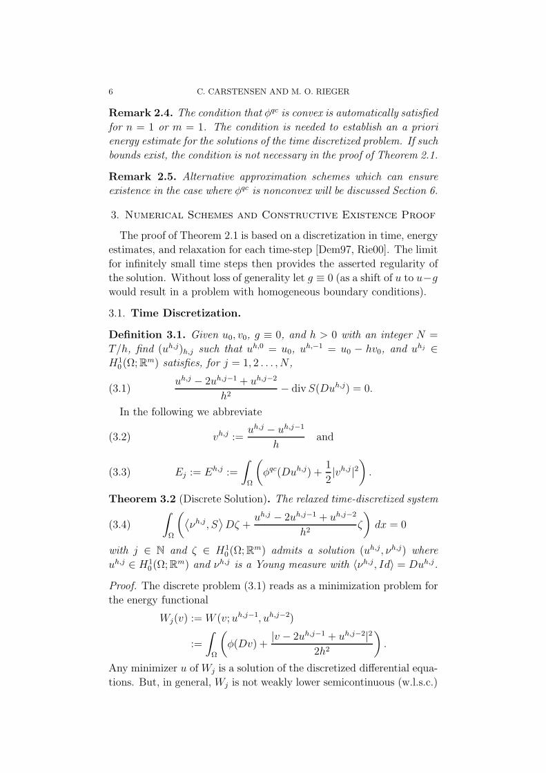
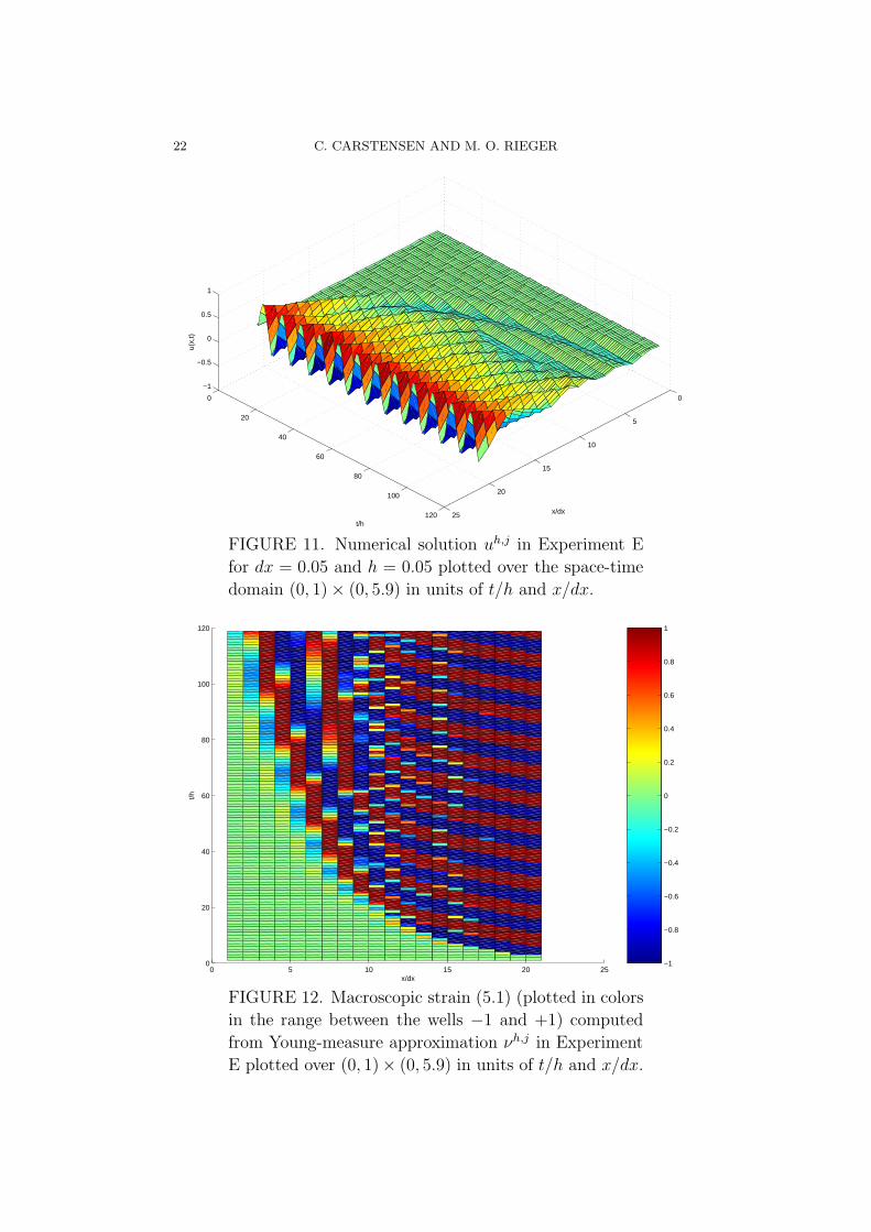
SIMULATIONS IN NON-MONOTONE ELASTODYNAMICS 21
experiments with oscillating boundary conditions we show an exam-
ple where the oscillating boundary condition are present over a longer
time. The resulting displacement and the deformation (see Fig. 11 and
Fig. 12) soon seem to approach a periodic solution, similar to the long
time calculations above.
5.3. Phase transition induced by temperature changes. The
third class of simulations concerns a time-dependent potential φ. This
models a shape memory alloy where the temperature is changed dur-
ing the experiment and passes a critical value, at which the type of φ
switches from nonconvex to convex or vice versa.
Experiment F. In this experiment we decrease the temperature
below the critical temperature, thus inducing a phase transition from
austenitic to martensitic phase. We choose the temperature-dependent
potential
φ(F, θ) := θ + min
1
2F 2 − θ,
1
2min(F − 1)2, (F + 1)2
,
where the temperature θ(t) is chosen as θ(t) := 0.2 − t, hence the
potential is changing from a 3-well to a 2-well potential. As initial
condition we choose
u0(x) := 0.1 sin(2πx) and v0 = 0.
We observe that the initial oscillations essentially continue, but with
decreasing amplitude. This seems to be an effect of the change in the
potential that takes energy out of the system. In view of the results of
Experiment G (see below), numerical viscosity as a source of the decay
in the amplitude can be excluded.
Experiment G. In the last experiment we consider the inverse sit-
uation: We start with a deformed wire. Its deformation is stable below
a certain temperature, but after passing this point it starts to oscillate.
We choose the temperature as θ(t) := t−0.1, and the initial conditions
as u0(x) := 0.1 sin(πx), u1 = 0. There is essentially no change in the
amplitude (unlike as in Experiment F). After passing the critical point,
the wire starts to oscillate as if released from a deformed initial state.
22 C. CARSTENSEN AND M. O. RIEGER
0
5
10
15
20
25
0
20
40
60
80
100
120
−1
−0.5
0
0.5
1
x/dx
t/h
u(x,
t)
FIGURE 11. Numerical solution uh,j in Experiment E
for dx = 0.05 and h = 0.05 plotted over the space-time
domain (0, 1) × (0, 5.9) in units of t/h and x/dx.
−1
−0.8
−0.6
−0.4
−0.2
0
0.2
0.4
0.6
0.8
1
0 5 10 15 20 250
20
40
60
80
100
120
x/dx
t/h
FIGURE 12. Macroscopic strain (5.1) (plotted in colors
in the range between the wells −1 and +1) computed
from Young-measure approximation νh,j in Experiment
E plotted over (0, 1)× (0, 5.9) in units of t/h and x/dx.

SIMULATIONS IN NON-MONOTONE ELASTODYNAMICS 23
0
10
20
30
40
50
0
10
20
30
40
50
−0.1
0
0.1
x/dxt/h
u(x,
t)
FIGURE 13. Numerical solution uh,j in Experiment F
for dx = 0.02 and h = 0.02 plotted over the space-time
domain (0, 1) × (0, 1) in units of t/h and x/dx.
0
10
20
30
40
50
0
10
20
30
40
50
60
−0.1
0
0.1
x/dxt/h
u(x,
t)
FIGURE 14. Numerical solution uh,j in Experiment G
for dx = 0.02 and h = 0.02 plotted over the space-time
domain (0, 1) × (0, 1) in units of t/h and x/dx.
24 C. CARSTENSEN AND M. O. RIEGER
6. Extensions
The condition φqc = φ∗∗ of Theorem 2.1 is, in general, difficult to
handle, since the quasiconvex envelope of a function is not easily ac-
cessible. A different characterization of this condition is given by the
following result due to Kewei Zhang.
Theorem 6.1 ([Zha02]). If φ : Rm×n → R is a C1-function and has
polynomial growth of order p > 1 at infinity and if φrc denotes the
rank-one-convexification of φ, then
φqc = φ∗∗ ⇔ φrc = φ∗∗. 2
For a given function φ the rank-one-convexification φrc can be calcu-
lated much easier than the quasiconvexification φqc. Hence this theorem
makes it feasible to test whether Theorem 2.1 can be applied for given
energy densities:
Corollary 6.2. If φ is rank-one-convex but not convex, then it does
not satisfy the assumptions of Theorem 2.1. 2
A similar result for a different time discretization scheme extends
Theorem 2.1 and is in particular applicable if φ is quasiconvex. On the
other hand it is not strictly more applicable than Theorem 2.1.
Theorem 6.3 (Existence). We define
φ(A1, A2) :=
∫ 1
0
1
s
(φ(sA1 + (1 − s)A2) − φ(A2)
)ds + φ(A2).
Let u0 ∈ H10 (Ω; Rm), v0 ∈ L2(Ω; Rm) and
(6.1) φqc(A1, A2)|A1=A2= φqc(A1).
Then there exists a Young measure solution (u, ν) of our problem that
can be obtained by the following time discretization scheme
uh,j − 2uh,j−1 + uh,j−2
h2− div S(Duh,j, Duh,j−1) = 0,
uh,0 = u0, uh,−1 = u0 − hv0,
where
S(A1, A2) :=
∫ 1
0
S(tA1 + (1 − t)A2) dt.
The discrete energy estimate can be proved for φ insetad of φ without
any convexity assumptions. The further existence proof follows closely
the proof of Theorem 2.1.

SIMULATIONS IN NON-MONOTONE ELASTODYNAMICS 25
-2 -1 1 2
-1
-0.5
0.5
1
1.5
2
Figure 6.15. Plot of the line l(A), the function h(A)
and the point (A2,−φ(A2)) in the range −2 ≤ A ≤+2. The line l apparently separates h and the point
(A2,−φ(A2)) (cf. Example 6.4).
Condition (6.1) appears technical. However, it is needed for taking
the final limit as the time-step size converges to zero. A sufficient
condition for (6.1) is that the energy density φ is quasiconvex.
We might ask whether condition (6.1) holds for general energy func-
tionals φ, but this is not true: The following example shows that, even
in simple non-quasiconvex situations, the envelope condition does not
always hold.
Example 6.4. Consider φ(A) := (1 − A2)2. Set A2 := 3/(2√
5) and
h(A1) := φ(A1, A2) − φ(A2). Then
h(A1) =1
400
(1485
4− 186
√5A1 − 310A2
1 + 40√
5A31 + 100A4
1
).
A line l separating the graph of h from the point (A2,−φ(A2)) is con-
structed as follows. Let l be defined by the two points (see Fig. 6.15)(−3
2, h
(−3
2
)− 5
100
)and
(1, h(1) − 5
100
).
The line l does not intersect the graph, and l(A2) > −φ(A2). Since
A2 < 1 and therefore φqc(A2) = 0 we derive
hqc(A2) + φ(A2) ≥ h∗∗(A2) + φ(A2) > 0 = φqc(A2),
and so
φqc(A1, A2)|A1=A2> φqc(A2).
Hence φ violates condition (6.1). 2

26 C. CARSTENSEN AND M. O. RIEGER
Acknowledgments. The research of CC was supported by the Max Planck
Institute for Mathematics in the Sciences, Leipzig, Germany, the Ger-
man Research Foundation through the DFG-Schwerpunktprogramm
multi-scale problems, and the Isaac Newton Institute of Mathematical
Sciences, Cambridge, UK; MOR was supported by Max Planck Insti-
tute for Mathematics in the Sciences and by the Center for Nonlinear
Analysis under NSF Grant DMS-9803791. He would like to thank Ste-
fan Muller for his constant support and helpful suggestions.
References
[BJ87] J. M. Ball and R. D. James. Fine phase mixtures as minimizers of energy.
Arch. Rational Mech. Anal., 100(1):13–52, 1987.
[BKK00] John M. Ball, Bernd Kirchheim, and Jan Kristensen. Regularity of qua-
siconvex envelopes. Calc. Var. Partial Differential Equations, 11(4):333–
359, 2000.
[BL73] Henri Berliocchi and Jean-Michel Lasry. Integrandes normales et mesures
parametrees en calcul des variations. Bull. Soc. Math. France, 101:129–
184, 1973.
[Car01] Carsten Carstensen. Numerical analysis of microstructure. In Theory and
numerics of differential equations (Durham, 2000), Universitext, pages
59–126. Springer Verlag, Berlin, 2001.
[CCK95] M. Chipot, C. Collins, and D. Kinderlehrer. Numerical analysis of oscil-
lations in multiple well problems. Numer. Math., 70(3):259–282, 1995.
[CD03] C. Carstensen and G. Dolzmann. Time-space discretization
of the nonlinear hyperbolic system utt = div(σ(Du) + Dut).
SIAM J. Numer. Analysis, 2003. In press. Preprint available at
http://www.mis.mpg.de/preprints/2001/prepr6001-abstr.html.
[CKL91] Charles Collins, David Kinderlehrer, and Mitchell Luskin. Numerical ap-
proximation of the solution of a variational problem with a double well
potential. SIAM J. Numer. Anal., 28(2):321–332, 1991.
[CL91] Charles Collins and Mitchell Luskin. Optimal-order error estimates for the
finite element approximation of the solution of a nonconvex variational
problem. Math. Comp., 57(196):621–637, 1991.
[CP97] Carsten Carstensen and Petr Plechac. Numerical solution of the scalar
double-well problem allowing microstructure. Math. Comp., 66(219):997–
1026, 1997.
[CR00] Carsten Carstensen and Tomas Roubıcek. Numerical approximation of
Young measures in non-convex variational problems. Numer. Math.,
84(3):395–415, 2000.
[Dem96] Sophia Demoulini. Young measure solutions for a nonlinear parabolic
equation of forward-backward type. SIAM J. Math. Anal., 27(2):376–403,
1996.
[Dem97] Sophia Demoulini. Young measure solutions for nonlinear evolutionary
systems of mixed type. Ann. Inst. H. Poincare Anal. Non Lineaire,
14(1):143–162, 1997.

SIMULATIONS IN NON-MONOTONE ELASTODYNAMICS 27
[DH85] Constantins M. Dafermos and William J. Hrusa. Energy methods for
quasilinear hyperbolic initial-boundary value problems. Applications to
elastodynamics. Arch. Rational Mech. Anal., 87(3):267–292, 1985.
[FD97] G. Friesecke and G. Dolzmann. Implicit time discretization and global
existence for a quasi-linear evolution equation with nonconvex energy.
SIAM J. Math. Anal., 28(2):363–380, 1997.
[KL94] P. Kloucek and M. Luskin. The computation of the dynamics of the
martensitic transformation. Contin. Mech. Thermodyn., 6(3):209–240,
1994.
[KP92] David Kinderlehrer and Pablo Pedregal. Weak convergence of integrands
and the Young measure representation. SIAM J. Math. Anal., 23(1):1–19,
1992.
[Lus96] Mitchell Luskin. On the computation of crystalline microstructure. In
Acta numerica, 1996, pages 191–257. Cambridge Univ. Press, Cambridge,
1996.
[Mul99] Stefan Muller. Variational models for microstructure and phase transi-
tion. In S. Hildebrandt and M. Struwe, editors, Calculus of Variations
and Geometric Evolution Problems, number 1713 in Lecture Notes in
Mathematics, page 211 ff. Springer Verlag, Berlin etc., 1999.
[NW93] R. A. Nicolaides and Noel J. Walkington. Computation of microstructure
utilizing Young measure representations. In Transactions of the Tenth
Army Conference on Applied Mathematics and Computing (West Point,
NY, 1992), pages 57–68. U.S. Army Res. Office, Research Triangle Park,
NC, 1993.
[Ped97] Pablo Pedregal. Parametrized measures and variational principles.
Birkhauser, 1997.
[Rie00] Marc Oliver Rieger. Time dependent Young measure solutions for an elas-
ticity equation with diffusion. In International Conference on Differential
Equations, Vol. 1, 2 (Berlin, 1999), pages 457–459. World Sci. Publish-
ing, River Edge, NJ, 2000.
[Rie03] Marc Oliver Rieger. Young measure solutions for nonconvex elastody-
namics. SIAM J. Math. Anal., 34(6):1380–1398, 2003.
[Rou97] Tomas Roubıcek. Relaxation in optimization theory and variational cal-
culus. Walter de Gruyter & Co., Berlin, 1997.
[RZ02] Marc Oliver Rieger and Johannes Zimmer. Global existence for noncon-
vex thermoelasticity. Preprint 30/2002, Center for Nonlinear Analysis,
Carnegie Mellon University, Pittsburgh, USA, 2002.
[Sle91] Marshall Slemrod. Dynamics of measured valued solutions to a backward-
forward heat equation. Journal of Dynamics and Differential Equations,
3(1):1–28, 1991.
[Tar79] L. Tartar. Compensated compactness and applications to partial differen-
tial equations. In Nonlinear analysis and mechanics: Heriot-Watt Sym-
posium, Vol. IV, pages 136–212. Pitman, Boston, Mass., 1979.
[Tay96] Michael E. Taylor. Partial Differential Equations III. Appl. Math. Sci-
ences 117. Springer Verlag, 1996.
[You37] L.C. Young. Generalized curves and the existence of an attained absolute
minimum in the calculus variations, volume classe III. 1937.

28 C. CARSTENSEN AND M. O. RIEGER
[You69] L. C. Young. Lectures on the calculus of variations and optimal control
theory. W. B. Saunders Co., Philadelphia, 1969.
[Zha02] Kewei Zhang. On some semiconvex envelopes. NoDEA Nonlinear Differ-
ential Equations Appl., 9(1):37–44, 2002.
Institute for Applied Mathematics and Numerical Analysis, Vienna
University of Technology, Wiedner Hauptstraße 8-10/115, A-1040
Wien, Austria
E-mail address : [email protected]
Scuola Normale Superiore, Piazza dei Cavalieri 7, 56100 Pisa, Italy
E-mail address : [email protected]
Copyright © 2022 FDOKUMEN