TimingTiming--Driven Placement Driven Placement Based on Monotone Cell Based on Monotone Cell Ordering ConstraintsOrdering Constraints

Chanseok Hwang and Chanseok Hwang and Massoud PedramMassoud Pedram

University of Southern CaliforniaUniversity of Southern CaliforniaDepartment of Electrical EngineeringDepartment of Electrical Engineering

Los Angeles CA, USALos Angeles CA, USA

OutlineOutline

TimingTiming--Driven PlacementDriven Placement––Problems & General MethodsProblems & General Methods

Our ApproachOur Approach––MotivationsMotivations––Preferred Signal DirectionsPreferred Signal Directions––PSDP AlgorithmPSDP Algorithm

Experimental ResultsExperimental ResultsConclusionConclusion

TimingTiming--Driven Placement (TDP)Driven Placement (TDP)

GoalGoalTo minimize the circuit delay while obtaining To minimize the circuit delay while obtaining a legal placement solutiona legal placement solutionChallengesChallenges–– Increasing dominance of Interconnect Increasing dominance of Interconnect

delay (50delay (50--70% of the longest path delay)70% of the longest path delay)–– Increasing circuit size (>10M gates)Increasing circuit size (>10M gates)

Solution Techniques for TDPSolution Techniques for TDP

PathPath--based Methodsbased Methods–– Consider inputConsider input--output paths during the problem output paths during the problem

formulationformulationMonitoring critical and nearMonitoring critical and near--critical pathscritical paths

–– Maintain accurate timing information during the Maintain accurate timing information during the optimizationoptimization

–– Suffer from high complexity and low scalability Suffer from high complexity and low scalability since the number of nearsince the number of near--critical paths can critical paths can become exponentially largebecome exponentially large

Solution Techniques (ContSolution Techniques (Cont ’’d)d)

NetNet--based Methodsbased Methods–– Run STA at intermediate steps of the placement Run STA at intermediate steps of the placement

processprocess–– Assign weights (or net length bounds) to timingAssign weights (or net length bounds) to timing--

critical nets according to their criticalitiescritical nets according to their criticalities–– Convert the TDP problem to a weighted wire Convert the TDP problem to a weighted wire

length minimization (or bounded wire length) length minimization (or bounded wire length) problemproblem

–– Suffer from the difficulty of identifying the proper Suffer from the difficulty of identifying the proper net weights and tend to exhibit poor net weights and tend to exhibit poor convergence for net reconvergence for net re--weighting (or result in weighting (or result in overover--constraining for net length bounding)constraining for net length bounding)

PSDP: Preferred Signal Direction PSDP: Preferred Signal Direction Driven PlacementDriven Placement

Starting from an initial placement solution, Starting from an initial placement solution, relying on a moverelying on a move--based optimization based optimization strategy, we assign a strategy, we assign a preferred signal preferred signal direction direction to each critical path in the circuit, to each critical path in the circuit, which in turn encourages the timingwhich in turn encourages the timing--critical critical cells on that path to move in a direction that cells on that path to move in a direction that would maximize the would maximize the monotonic behaviormonotonic behavior of of the path in the 2the path in the 2--D placement solution.D placement solution.This is based on our observation that most This is based on our observation that most of paths causing timing problems in a circuit of paths causing timing problems in a circuit meander outside the minimum bounding meander outside the minimum bounding box of the start and end nodes of the path.box of the start and end nodes of the path.

Monotone Cell OrderingMonotone Cell Ordering

Flip-flops

Combinationallogic gates

Non-monotone cell order ing Monotone cell order ing

Cells on a target path do not zigzag or Cells on a target path do not zigzag or crisscross when the physical path from input crisscross when the physical path from input to output is traced.to output is traced.–– Previously used for wire planning during Previously used for wire planning during

synthesis and for net list partitioning.synthesis and for net list partitioning.

Related Work on Signal Related Work on Signal Directions and Monotone PathsDirections and Monotone Paths

S. S. ImanIman, M. Pedram, C. Fabian, and J. Cong, , M. Pedram, C. Fabian, and J. Cong, ““Finding Finding uniuni--directional cuts based on physical partitioning and logic directional cuts based on physical partitioning and logic restructuringrestructuring””, IWPD, 1993., IWPD, 1993.W. W. GostiGosti, A. , A. NarayanNarayan, R. K. , R. K. BraytonBrayton and A. L. and A. L. SangivanniSangivanni--VincentelliVincentelli, , ““Wire planning in Logic SynthesisWire planning in Logic Synthesis””, ICCAD, ICCAD, , 19981998..Cong and Lim, Cong and Lim, ““Performance Driven MultiPerformance Driven Multi--way way PartitioningPartitioning””, ASP, ASP--DAC, 2000.DAC, 2000.A. B. A. B. KahngKahng and X. and X. XuXu, , ““Local Unidirectional Bias for Local Unidirectional Bias for Smooth Smooth CutsizeCutsize--Delay Tradeoff in PerformanceDelay Tradeoff in Performance--driven driven bipartitioningbipartitioning..”” ISPD, 2003.ISPD, 2003.C. Hwang and M. Pedram, C. Hwang and M. Pedram, ““PMP: PerformancePMP: Performance--driven driven multilevel partitioning by aggregating the preferred signal multilevel partitioning by aggregating the preferred signal directions of I/O conduitsdirections of I/O conduits””, ASP, ASP--DAC, 2005.DAC, 2005.

Path Grouping and I/O ConduitsPath Grouping and I/O Conduits

To make the direction assignment tractable, we implicitly group all circuit paths into a set of input-output conduits and assign a unique preferred direction to each such conduit.

DefinitionDefinition–– I/O conduit I/O conduit : : the set of all paths from some the set of all paths from some PI PI

(or (or FFFF) to some ) to some PO PO (or (or FFFF))

NNI/OI/O conduitsconduits = (= (NNPIPI + N+ NFFFF) * (N) * (NPOPO + N+ NFFFF))

Preferred Signal Directions of Preferred Signal Directions of I/O ConduitsI/O Conduits

All paths in All paths in satisfy the monotone cell satisfy the monotone cell ordering property (resulting in minimum ordering property (resulting in minimum wire delay), if the preferred signal direction wire delay), if the preferred signal direction is satisfied for all edges in the is satisfied for all edges in the I/O conduit.I/O conduit.

DefinitionDefinition–– Preferred signal direction of Preferred signal direction of SDSD(( )):: one of the one of the

following directions, following directions, LLLL, , LRLR, , RLRL and and RR,RR,depending on the locations of depending on the locations of PIPI and and PO PO ofof ..

Signal Direction ConstraintsSignal Direction Constraints

Signal direction constraints for the vertical move line:P(s(ei)) P(t(ei)), 1 i 7 for 1 // SD( 1) = LRP(s(ei)) = P(t(ei)) = 0, 8 i 10 for 2 // SD( 2) = LL

s(ei): Source node of eit(ei): Target node of eiP(vi): Part number (0 or 1) of vi

1 : pi1 v1 v2 v3 po1e1(pi1,v1), e2(v1,v2), e3(v2,v3), e4(v3,po1)

2 : pi2 v6 v7 po2e8(pi2,v6), e9(v6,v7), e10(v7,po2)

pi1 v1 v4 v5 po1e1(pi1,v1), e5(v1,v2), e6(v2,v3), e7(v3,po1)

V4V3

V7V5

Vertical move line

Part0 Part1

po2

pi2

po1

V6

pi1V2

V1

Signal Direction Constraint Signal Direction Constraint (Cont(Cont ’’d)d)

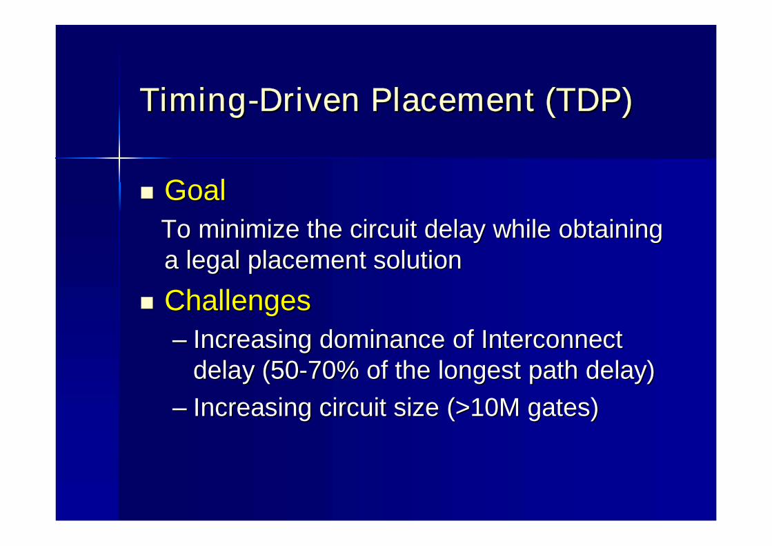
Signal direction constraint for a VERT (HORZ) move line

SDC1: if SD( ) = LL (BB), ei , P(s(ei)) = P(t(ei)) = 0 SDC2: if SD( ) = RR (TT), ei , P(s(ei)) = P(t(ei)) = 1 SDC3: if SD( ) = LR (BT), ei , P(s(ei)) P(t(ei)) SDC4: if SD( ) = RL (TB), ei , P(s(ei)) P(t(ei))

DifficultyDifficulty–– No solution that satisfies No solution that satisfies SDCsSDCs of all I/O of all I/O

conduits exists.conduits exists.–– Increases the total wire length.Increases the total wire length.

SolutionSolution–– SDCSDC’’ss need to be relaxed.need to be relaxed.

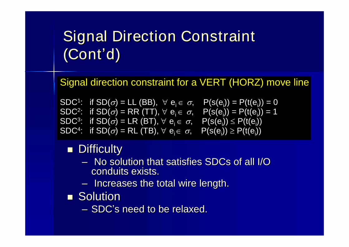
We treat delay as an optimization objective We treat delay as an optimization objective instead of a hard constraint to be satisfied, instead of a hard constraint to be satisfied, and use theand use the violation count violation count of of SDCSDC’’ss..–– Timing gain functionTiming gain function, , TG(vTG(vii)), is defined to , is defined to

quantitatively evaluate the desirability of moving quantitatively evaluate the desirability of moving vviifrom part_0 to part_1. It is calculated as:from part_0 to part_1. It is calculated as:

SD Violation Count as the Timing SD Violation Count as the Timing Gain Function for a Cell MoveGain Function for a Cell Move

TG(vTG(vii)) = = VCVC((vvii | | PP((vvii)=0) )=0) –– VCVC((vvii | | PP((vvii)=1))=1)

VC(vVC(vii | | P(vP(vii)): violation counts of SDC when P(v)): violation counts of SDC when P(vii) is 0 or 1) is 0 or 1

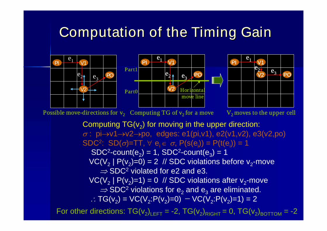
Computation of the Timing GainComputation of the Timing Gain

V1

V2

PO

PI

Possible move-directions for v2

e1

e2 e3

Computing TG(v2) for moving in the upper direction:: pi v1 v2 po, edges: e1(pi,v1), e2(v1,v2), e3(v2,po)

SDC2: SD( )=TT, ei , P(s(ei)) = P(t(ei)) = 1SDC2-count(e2) = 1, SDC2-count(e3) = 1

VC(V2 | P(v2)=0) = 2 // SDC violations before v2-moveSDC2 violated for e2 and e3.

VC(V2 | P(v2)=1) = 0 // SDC violations after v2-moveSDC2 violations for e2 and e3 are eliminated.

TG(v2) = VC(V2:P(v2)=0) − VC(V2:P(v2)=1) = 2

V2 PO

PI

V2 moves to the upper cell

e1

e2 e3

V1

For other directions: TG(v2)LEFT = -2, TG(v2)RIGHT = 0, TG(v2)BOTTOM = -2

Hor izontalmove line

V1

V2

PO

PI

Computing TG of v2 for a move

e1

e3

Par t0

Par t1 e2

Aggregating the SD Violation Aggregating the SD Violation CountsCounts

The timing gain of a node The timing gain of a node vvii w.r.tw.r.t. a target move . a target move direction is obtained by summing the number of direction is obtained by summing the number of SDVSDV’’ss of each edge of each edge eejj connected to nodeconnected to node vvii ..This calculation is done by considering all I/O This calculation is done by considering all I/O conduits (with given preferred signal directions) conduits (with given preferred signal directions) that go through the edge that go through the edge eejj ..We thus aggregate preferred signal directions We thus aggregate preferred signal directions for all critical paths that pass through an edge, for all critical paths that pass through an edge, which in turn enables us to maximize the which in turn enables us to maximize the monotonic behavior of the critical paths.monotonic behavior of the critical paths.

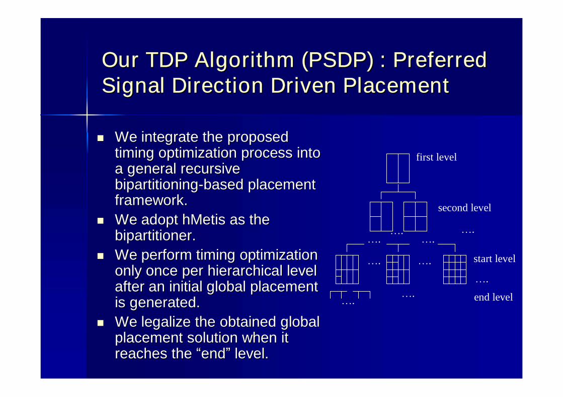
Our TDP Algorithm (PSDP) : Preferred Our TDP Algorithm (PSDP) : Preferred Signal Direction Driven PlacementSignal Direction Driven Placement

We integrate the proposed We integrate the proposed timing optimization process into timing optimization process into a general recursive a general recursive bipartitioningbipartitioning--based placement based placement framework.framework.We adopt We adopt hMetishMetis as the as the bipartitionerbipartitioner..We perform timing optimization We perform timing optimization only once per hierarchical level only once per hierarchical level after an initial global placement after an initial global placement is generated.is generated.We legalize the obtained global We legalize the obtained global placement solution when it placement solution when it reaches the reaches the ““endend”” level.level.

first level

second level

….

start level

….

….

….….

…. ….

end level….….

PSDP AlgorithmPSDP Algorithm

PSD_Placement (PSD_Placement (GG, , TT))GG : A directed graph representing a sequential circuit: A directed graph representing a sequential circuitTT : Timing constraints: Timing constraints1. Calculate the start and end levels of timing1. Calculate the start and end levels of timing--driven global driven global placement;placement;2. Do initial wirelength2. Do initial wirelength--driven global placement from level one to driven global placement from level one to start level;start level;3. While (start_level 3. While (start_level ≤≤ ii ≤≤ end_level)end_level)

•• While (While (jj=0; =0; jj < number of sub_regions in level < number of sub_regions in level i; j++i; j++))•• Generate a bipartitioningGenerate a bipartitioning--based placement based placement PPi,ji,j of of

sub_region sub_region jj;;•• Do Do Timing_Optimization_PSD(Timing_Optimization_PSD(PPii ,,TT););

4. Do the legalization;4. Do the legalization;

PSDP Algorithm (ContPSDP Algorithm (Cont ’’))

Timing _Optimization_PSD (P,T)P : An initial hierarchical placement solution with J regionsT : Timing constraints1. Perform static timing analysis;2. Find critical nodes, edges and I/O conduits;3. Compute initial timing gains for all critical nodes;4. Put all critical nodes into a timing gain heap;5. While (heap != empty)

• Extract root node vi from the heap and move it in its preferred direction to a neighbor region in P;• If the region capacity is violated, select a non-critical node in the region and move it back to the parent region of vi;• Update timing gains and restructure the heap as needed;

6. Find a sequence of moves that produces max_total_gain;7. Undo moves that are not in the selected sequence;8. If max_total_gain > 0 then goto step 3;9. Else exit;

Experimental SetupExperimental Setup

6 test cases; four (6 test cases; four (matrix, vp2, mac1 and mac2matrix, vp2, mac1 and mac2) are ) are obtained from ISPD 2001 benchmarks while the obtained from ISPD 2001 benchmarks while the other two (other two (indust1 and indust2indust1 and indust2) are from a partner ) are from a partner ASIC company.ASIC company.

The delay models are based on The delay models are based on TSMCTSMC 0.180.18umumtechnology.technology.

PSDPPSDP is compared with is compared with CapoCapo--boostboost and and a leading a leading industry placement toolindustry placement tool (called (called QuadPQuadP) in terms of ) in terms of wire length and worst negative slack.wire length and worst negative slack.

We use Cadence We use Cadence WarpRouteWarpRoute and and PearlPearl to report to report the experimental results.the experimental results.

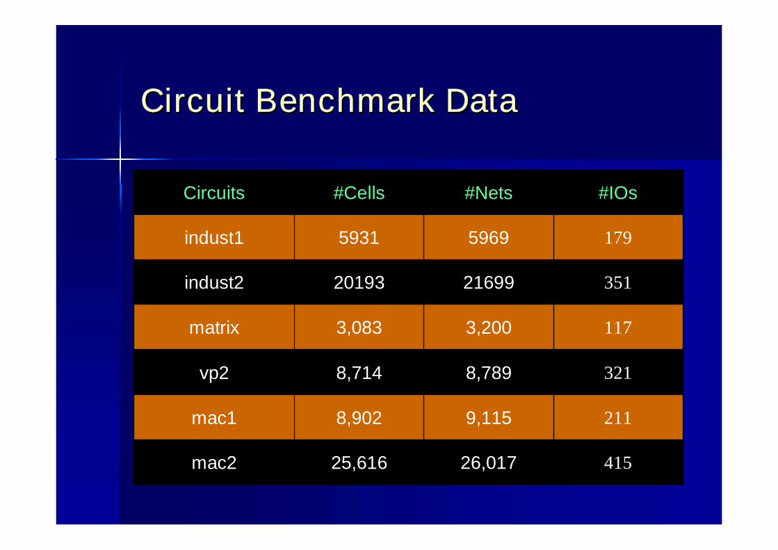
Circuit Benchmark DataCircuit Benchmark Data

41526,01725,616mac2

2119,1158,902mac1

3218,7898,714vp2

1173,2003,083matrix

3512169920193indust2

17959695931indust1

#IOs#Nets#CellsCircuits

Experimental ResultsExperimental Results

44.5%Average50.2%-62.7-125.42.35mac2

36.9%-13.5-21.42.07mac1

63.3%-25.1-68.33.67vp2

25.9%-4.3-5.83.23matrix

54.5%-93.1-204.58.75indust2

36.1%-24.4-38.25.54indust1

% Improvement

Timing-driven mode

Wirelength-driven mode

Clock cycle

Benchmark circuits

Comparisons of TNS (Comparisons of TNS (total negative slacktotal negative slack of all of all timing endpoints) between wirelengthtiming endpoints) between wirelength--driven and driven and timingtiming--driven modes of PSDPdriven modes of PSDP

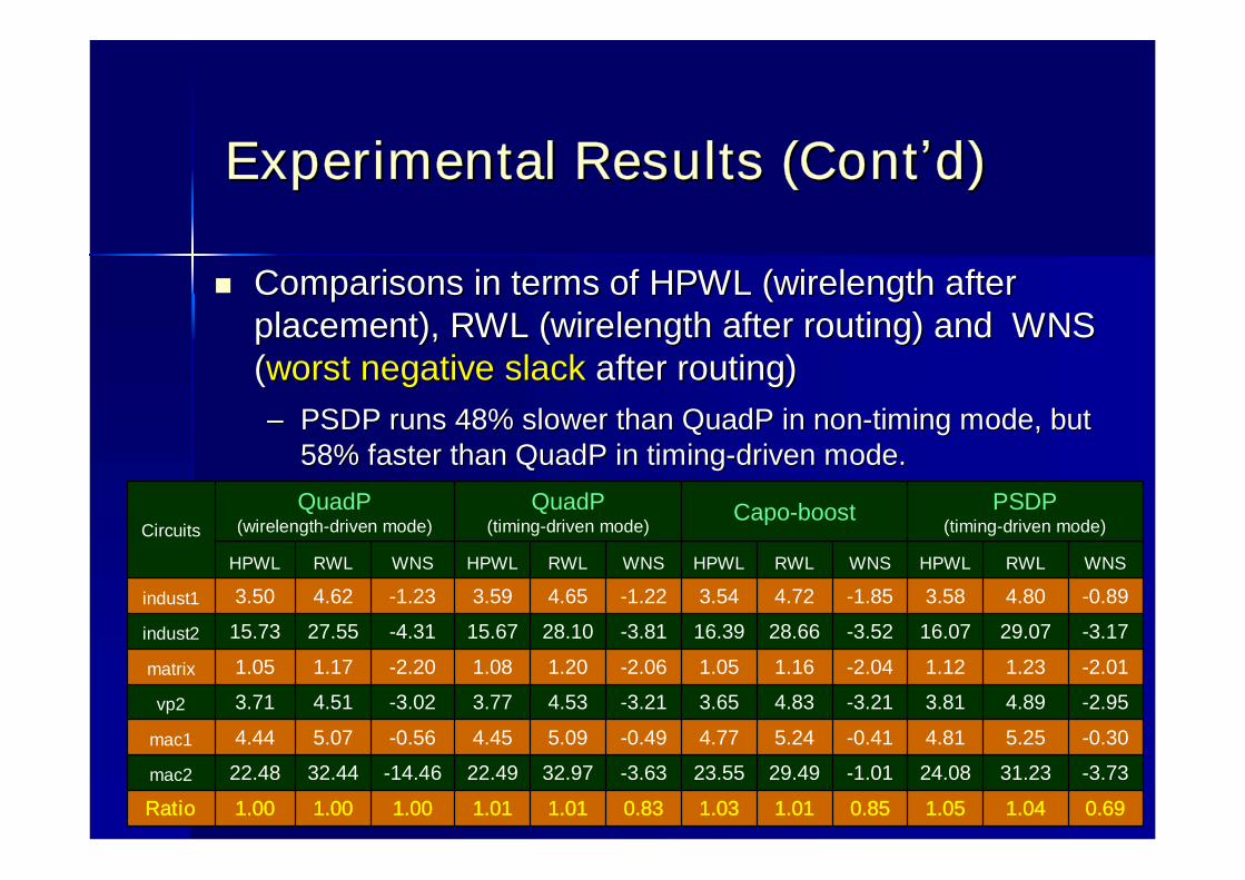
Experimental Results (ContExperimental Results (Cont ’’d)d)

Comparisons in terms of HPWL (wirelength after Comparisons in terms of HPWL (wirelength after placement), RWL (wirelength after routing) and WNS placement), RWL (wirelength after routing) and WNS ((worst negative slackworst negative slack after routing)after routing)–– PSDP runs 48% slower than QuadP in nonPSDP runs 48% slower than QuadP in non--timing mode, but timing mode, but

58% faster than QuadP in timing58% faster than QuadP in timing--driven mode.driven mode.

0.691.041.050.851.011.030.831.011.011.001.001.00Ratio

-3.7331.2324.08-1.0129.4923.55-3.6332.9722.49-14.4632.4422.48 mac2

-0.305.25 4.81-0.415.24 4.77 -0.495.094.45 -0.565.07 4.44mac1

-2.954.893.81-3.214.83 3.65 -3.214.533.77-3.024.513.71 vp2

-2.011.23 1.12-2.041.16 1.05-2.061.201.08-2.201.171.05matrix

-3.1729.0716.07-3.5228.6616.39-3.8128.1015.67-4.3127.5515.73indust2

-0.894.803.58-1.854.723.54-1.224.653.59-1.234.623.50indust1

WNSRWLHPWLWNSRWLHPWLWNSRWLHPWLWNSRWLHPWL

PSDP(timing-driven mode)

Capo-boostQuadP(timing-driven mode)

QuadP(wirelength-driven mode)Circuits

ConclusionsConclusions

We introduced a new timingWe introduced a new timing--gain function gain function model based on preferred signal directions model based on preferred signal directions for the timingfor the timing--driven placement context.driven placement context.The advantage of the new methodology has The advantage of the new methodology has been confirmed by experimental results: on been confirmed by experimental results: on average 31% improvement on WNS. average 31% improvement on WNS. compared to a leading industry placer at the compared to a leading industry placer at the expense of expense of wirelengthwirelength increase, on average, increase, on average, by 5%.by 5%.