Delta function approximations in level set methods by distance ...

Journal of Computational Physics 229 (2010) 2199–2219

Contents lists available at ScienceDirect

Journal of Computational Physics

journal homepage: www.elsevier .com/locate / jcp

Delta function approximations in level set methods by distancefunction extension

Sara Zahedi *, Anna-Karin TornbergSchool of Computer Science and Communication, Royal Institute of Technology, SE-100 44 Stockholm, Sweden

a r t i c l e i n f o

Article history:Received 1 June 2009Received in revised form 10 November 2009Accepted 19 November 2009Available online 27 November 2009

Keywords:Level set methodDelta functionConsistent approximationsDiscretizationDistance function

0021-9991/$ - see front matter � 2009 Elsevier Incdoi:10.1016/j.jcp.2009.11.030

* Corresponding author.E-mail addresses: [email protected] (S. Zahedi), anna

a b s t r a c t

In [A.-K. Tornberg, B. Engquist, Numerical approximations of singular source terms in dif-ferential equations, J. Comput. Phys. 200 (2004) 462–488], it was shown for simple exam-ples that the then most common way to regularize delta functions in connection to levelset methods produces inconsistent approximations with errors that are not reduced withgrid refinement. Since then, several clever approximations have been derived to overcomethis problem. However, the great appeal of the old method was its simplicity. In this paperit is shown that the old method – a one-dimensional delta function approximationextended to higher dimensions by a distance function – can be made accurate with a dif-ferent class of one-dimensional delta function approximations. The prize to pay is a widersupport of the resulting delta function approximations.

� 2009 Elsevier Inc. All rights reserved.

1. Introduction

The level set method, originally devised by Osher and Sethian [1], is a very popular method for the evolution of interfaces,and it has been implemented for numerous applications. In some of these applications, the question of how to numericallyapproximate a Dirac delta function arises. For example, in immiscible multiphase problems, Dirac delta functions supportedon interfaces separating different fluids are often used in the modeling of the surface tension forces acting on the interfaces.Another example is the problem of evaluating a line integral in two dimensions or a surface integral in three dimensions.This problem can conveniently be reformulated as an integral in 2D or 3D involving a Dirac delta function with supporton the line or surface. One approach to approximate such delta functions is to extend a regularized one-dimensional deltafunction to higher dimensions using a distance function. This has been a common technique in connection to level set meth-ods [2] since the distance function is usually available discretized on a computational grid. However, care is needed since theextension to higher dimensions using a distance function may lead to Oð1Þ errors [3]. In [3], it was shown that another exten-sion technique that is based on products of regularized one-dimensional delta functions [4] is consistent. This technique ishowever only applicable when an explicit representation of the curve or the surface is available. In level set methods thecurve or the surface is represented implicitly by a level set [2,5].

To overcome the lack of consistency that became apparent with the work presented in [3], a number of consistent deltafunction approximations that can be used with level set methods have been proposed. Engquist et al. [6] proposed two suchapproximations. The first one is an approximation of the product rule using the distance function and its gradient. The sec-ond one is based on the linear hat function but uses a variable regularization parameter. Smereka [7] derived a discrete deltafunction obtained as the truncation error in solving the Laplacian of the Green’s function, which was proven to be second-order accurate by Beale [8]. Consistent approximations for which the level set function and its gradient are needed have also

. All rights reserved.

[email protected] (A.-K. Tornberg).

http://dx.doi.org/10.1016/j.jcp.2009.11.030

mailto:[email protected]

mailto:[email protected]

http://www.sciencedirect.com/science/journal/00219991

http://www.elsevier.com/locate/jcp

2200 S. Zahedi, A.-K. Tornberg / Journal of Computational Physics 229 (2010) 2199–2219

been introduced by Towers [9,10]. The advantage of these methods is that the supports of the delta function approximationsare very small. The discrete delta function proposed by Smereka has its support contained within a single mesh cell.

One way to explain the reason for the inconsistency shown in [3] is the following: The one-dimensional delta functionapproximation is designed to obey certain moment conditions on a uniform grid. The first moment condition is the masscondition that ensures that the delta function approximation sums to one independent of shifts in the grid. Delta functionapproximations with compact support where the widths of the approximations are fixed to a number of cell widths was con-sidered in [3]. As the one-dimensional delta function is extended to higher dimensions, using the closest distance to the lineor surface, the effective width in each coordinate direction relative to the grid size will depend on the slope of the curve orsurface. This will in general no longer be within the design of the one-dimensional delta approximation, causing a violationof the mass condition, and hence an Oð1Þ error that will not vanish with grid refinement. This is further discussed in Section 3.This effect was recognized by Engquist et al. [6] who introduced a first correction to this, by defining the regularizationparameter to depend on the gradient of the distance function.

The problem with extending the delta function to higher dimensions using the closest distance to the line or surface ishence that the one-dimensional delta approximation is dilated, and that the moment conditions are no longer valid. Onecan however construct delta approximations such that the moment conditions do hold for a wide range of dilations. Thesefunctions are however not of compact support. One such function was given in [11]. It has compact support in Fourier space,and decays rapidly enough in real space to lend itself to truncation, but the effective support will be wider than one or twogrid points as in the approximations above. In addition, in difference to the delta function approximations discussed above,that are of low regularity, this function is infinitely differentiable.

In the analysis in [12], the error is split into two parts. The first part is the analytical error due to the approximation of thedelta function. The second part is the numerical error due to the approximation of the integral containing the delta functionapproximation. For the first part, it is continuous moment conditions that are important, and for the second part, it is (inaddition to the order of the quadrature rule) the regularity of the delta function approximation that limits the accuracy. Thisgives an upper limit of the error, but in the case when extending by the distance rule, the error is typically quite close to thisupper limit. The result from this analysis is that the numerical error is of order Oððh=eÞpÞ where p is determined by the reg-ularity of the delta function approximation. For the compact one-dimensional delta function approximation, the regularity istypically low. With a choice of e ¼ mh, which has been the common choice, the numerical error is of Oð1Þ, and the method isinconsistent. Depending on the regularity and continuous moment order of the approximation, there is an optimal a < 1 ine � ha that results in the best convergence. If we replace the narrow delta function approximation with an infinitely differ-entiable delta function approximation, the result is quite different. The regularity of the delta function approximation will nolonger limit the accuracy of the quadrature rule. In fact, these functions can be considered as periodic functions, since theydecay to zero. For these functions, the trapezoidal rule on a uniform grid will converge faster than any power of h in the limitas h! 0. This is often referred to as the superconvergence of the trapezoidal rule, and will yield a very small numerical error.

In this paper, we will consider three different functions that all have these properties. We will now provide a comparisonbetween one of the delta function approximations considered in this paper and the narrow linear hat function which in [3]was shown to give Oð1Þ errors. Consider the computation of the arc-length of a circle of radius 1 centered at the origin byevaluating
Z
XdeðdðC; xÞÞdX;

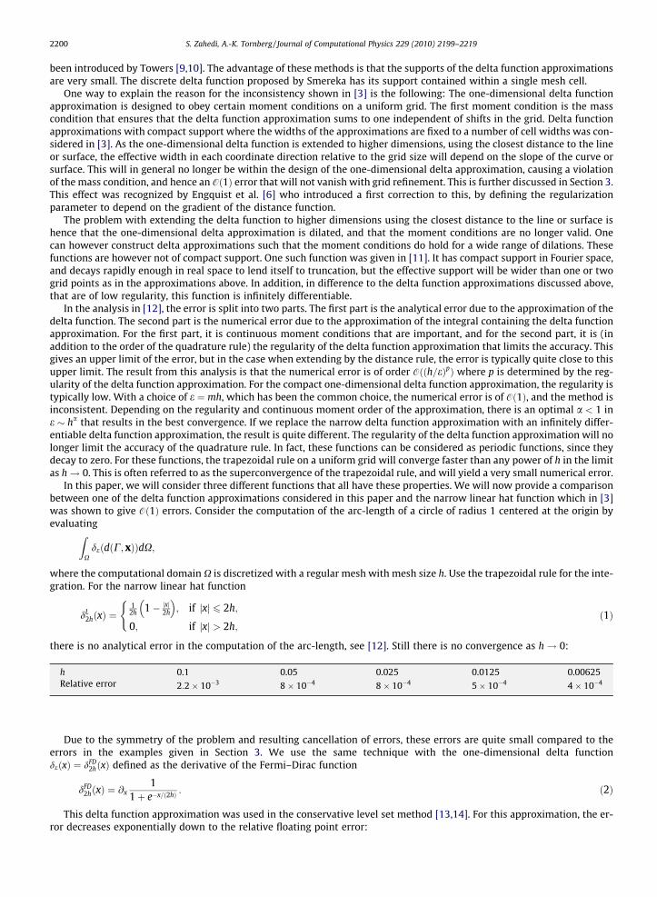
where the computational domain X is discretized with a regular mesh with mesh size h. Use the trapezoidal rule for the inte-gration. For the narrow linear hat function

dL2hðxÞ ¼

12h 1� jxj2h

� �; if jxj 6 2h;

0; if jxj > 2h;

(ð1Þ

there is no analytical error in the computation of the arc-length, see [12]. Still there is no convergence as h! 0:

h
0.1 0.05 0.025 0.0125 0.00625 Relative error 2:2� 10�3 8� 10�4 8� 10�4 5� 10�4 4� 10�4
Due to the symmetry of the problem and resulting cancellation of errors, these errors are quite small compared to theerrors in the examples given in Section 3. We use the same technique with the one-dimensional delta functiondeðxÞ ¼ dFD

2hðxÞ defined as the derivative of the Fermi–Dirac function

dFD2hðxÞ ¼ @x

11þ e�x=ð2hÞ : ð2Þ

This delta function approximation was used in the conservative level set method [13,14]. For this approximation, the er-ror decreases exponentially down to the relative floating point error:

Fi

S. Zahedi, A.-K. Tornberg / Journal of Computational Physics 229 (2010) 2199–2219 2201

h

−2 −1 0

0

0.5

1

1.5

2

g. 1. Building blocks uðnÞ for d

0.1

1 2 −2

0

0.5

1

1.5

2

elta function approximatio

0.05

−1 0

ns. A linear hat function (

0.025

1 2 −2

0

0.5

1

1.5

2

a), a cosine approximation

0.0125

−1 0 1

(b), and a piecewise cubic

0.00625
Relative error 4:4� 10�3 2� 10�5 7� 10�10 1� 10�14 4� 10�15
What we see is the superconvergence of the trapezoidal rule for infinitely differentiable periodic functions.This paper is organized as follows. In Section 2 we define delta function approximations and state conditions for accuracy

in one dimension. In Section 3 we discuss the simple example of computing the length of a line. We show why the compactdelta function approximations produce Oð1Þ errors and how large they are. We also show why this does not occur for approx-imations with compact support in Fourier space. In Section 4 we introduce three different consistent delta function approx-imations and discuss their properties. In Section 5 we state and prove theorems for the error in both two and threedimensions. We present numerical experiments in Section 6 and summarize our results in Section 7.

2. Regularization

Given a continuous function uðnÞ, a delta function approximation can be constructed by

deðxÞ ¼1euðx=eÞ: ð3Þ

Examples of such uðnÞ functions with compact support are: the piecewise linear hat function

uLðnÞ ¼ð1� jnjÞ; if jnj 6 1;0; if jnj > 1;

�ð4Þ

the cosine approximation

ucosðnÞ ¼12 ð1þ cosðpnÞÞ; if jnj 6 1;0; if jnj > 1;

(ð5Þ

and the piecewise cubic function

uCðnÞ ¼2� j2nj � 2j2nj2 þ j2nj3; if 0 6 jnj 6 1=2;

2� 113 j2nj þ 2j2nj2 � 1

3 j2nj3; if 1=2 < jnj 6 1;0; if jnj > 1:

8><>: ð6Þ

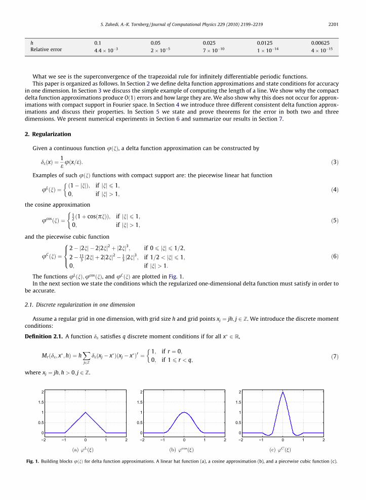
The functions uLðnÞ;ucosðnÞ, and uCðnÞ are plotted in Fig. 1.In the next section we state the conditions which the regularized one-dimensional delta function must satisfy in order to

be accurate.

2.1. Discrete regularization in one dimension

Assume a regular grid in one dimension, with grid size h and grid points xj ¼ jh; j 2 Z. We introduce the discrete momentconditions:

Definition 2.1. A function de satisfies q discrete moment conditions if for all x� 2 R,

Mrðde; x�;hÞ ¼ hXj2Z

deðxj � x�Þðxj � x�Þr ¼1; if r ¼ 0;0; if 1 6 r < q;

�ð7Þ

where xj ¼ jh; h > 0; j 2 Z.

2

function (c).


If de satisfies q moment conditions, we say that it has a moment order q. The first moment condition ensures that the massof the delta function approximation de is one, independent of shifts in the grid. It is therefore referred to as the mass con-dition. The higher moment conditions are important when the delta approximation is multiplied by a non-constant function.The following theorem states that in one dimension the numerical accuracy of a regularized delta function is determined bythe number of discrete moment conditions.

Proposition 2.1. Assume de satisfies q discrete moment conditions and has compact support in ½�Mh;Mh�. Assume also thatf ðxÞ 2 CqðRÞ, and that all derivatives of f are bounded, then

E ¼ hX

j

deðxj � x�Þf ðxjÞ � f ðx�Þ��

�� 6 Chq ð8Þ

and E ¼ 0 if f is constant.

A proof based on Taylor expansion of f around x� 2 R is found in Refs. [3,15]. The delta function approximations de in lastsection have support in ½�e; e�. The linear hat function dL

2hðxÞ, the cosine approximation dcos2h ðxÞ and the cubic function dC

2hðxÞ allsatisfy the mass condition and hence are consistent approximations. The cubic function dC

2hðxÞ is most accurate. It satisfiesfour discrete moment conditions and is according to Proposition 2.1 a fourth-order accurate approximation.

2.2. Extensions to higher dimensions

A Dirac delta measure concentrated on a curve or surface can be approximated by extending a regularized one-dimen-sional delta function to higher dimensions. Basically two techniques are used. One is the product formula and the other tech-nique is based on a distance function to the curve or the surface.

Let C � Rd be a d� 1 dimensional closed, continuous, and bounded surface and let S be a parametrization of C. DefinedðC; g;xÞ as a delta function of variable strength supported on C such that
Z
RddðC; g; xÞf ðxÞdx ¼

ZC

gðSÞf ðXðSÞÞdS; ð9Þ

where x ¼ ðxð1Þ; . . . xðdÞÞ 2 Rd and XðSÞ ¼ ðXð1ÞðSÞ; . . . ;XðdÞðSÞÞ 2 C.The product formula yields

deðC; g;xÞ ¼Z

C

Yd

k¼1

dekðxðkÞ � XðkÞðSÞÞgðSÞdS; ð10Þ

where dekis a one-dimensional regularized delta function.

Assume that the space Rd is covered by a regular grid

fxjgj2Zd ; xj ¼ xð1Þj1; . . . ; xðdÞjd

� �; xðkÞjk

¼ xðkÞ0 þ jkhk; jk 2 Z; k ¼ 1; . . . ;d: ð11Þ

The following theorem was proved by Tornberg and Engquist in Ref. [3].

Theorem 2.1. Suppose that de is a one-dimensional delta function approximation with compact support in ½�e; e�, that satisfies qdiscrete moment conditions (see Definition 2.1); g 2 CrðRdÞ and f 2 CrðRdÞ; r P q. Then for any rectifiable curve C and deðC; g;xÞas defined in Eq. (10) with e ¼ ðmh1;mh2; . . . ;mhdÞ, it holds that

E ¼Yd

k¼1

hk

!Xj2Zd

deðC; g;xjÞf ðxjÞ �Z

CgðSÞf ðXðSÞÞdS

�� 6 Chq ð12Þ

with h ¼max16k6dhk and E ¼ 0 for constant f.

This means that the results from one dimension carry over to higher dimensions, and that it is still the discrete momentorder of the one-dimensional delta function approximation that determines the order of accuracy.

The product formula is easy to use when C is explicitly defined. However, in level set methods, C is defined implicitly by alevel set function /ðxÞ : Rd ! R,

C ¼ fx : /ðxÞ ¼ 0g: ð13Þ

It is therefore preferable to use this function to extend the regularized one-dimensional delta function de to higher dimen-sions. In the case when /ðxÞ ¼ dðC;xÞ, a signed distance function to C, where the distance is the Euclidean distance from x toC, the delta function approximation is defined as

deðC; g;xÞ ¼ ~gðxÞdeðdðC;xÞÞ; ð14Þ

where ~g is a smooth extension of g to Rd, such that ~gðXðSÞÞ ¼ gðSÞ. Using the level set function the integral in Eq. (9) can bewritten as

ZRd
f ðxÞdðC; g; xÞdx ¼Z

Rdf ðxÞ~gðxÞdð/ðxÞÞjr/ðxÞjdx: ð15Þ

Note that the extra scaling of jr/j is needed when / is not a distance function. In this paper we focus on the extension tohigher dimensions that employs the distance function.

3. Computing the length of a straight line

In this section we study the error made in the computation of the length of a straight line. In the computations a regu-larized one-dimensional delta function de is extended to higher dimensions using a distance function, according to Eq. (14)with ~g ¼ 1.

Consider the problem of calculating the length of a curve C:

jCj ¼ S ¼Z

R2dðC;xÞdx: ð16Þ

In the computation of jSj, a delta function approximation de on a regular grid is used:

Sh ¼ h2Xj2Z2

deðdðC;xjÞÞ; xj ¼ ðxj1 ; yj2Þ; xj1 ¼ j1h; yj2

¼ j2h; jl 2 Z; l ¼ 1;2: ð17Þ

In the following we will let the curve C 2 R2 be a straight line with slope k, but not a vertical line or a horizontal line. InRef. [3] it was shown that for C ¼ fx; xð2Þ ¼ xð1Þ;0 6 xð1Þ < S=

ffiffiffi2pg, a line with slope k ¼ 1 and de being equal to the narrow

linear hat function dLh the relative error jSh � Sj=S is more than 12% as h! 0. This was shown by dividing the sum Sh into

contributions of M subsegments of C, each of lengthffiffiffi2p

h. Here, we consider a different approach. We express the error interms of the first discrete moment of de (see Eq. (7) with r ¼ 0). We can then show which delta function approximations thatwill produce Oð1Þ errors. For simplicity, we consider a line of infinite length so we do not have to worry about contributionsfrom end point terms.

From Eq. (3) we see that we can write deðxÞ as

deðxÞ ¼ gd~eðgxÞ; ~e ¼ ge: ð18Þ

We take

g ¼ 1k

ffiffiffiffiffiffiffiffiffiffiffiffiffiffi1þ k2

q; ð19Þ

where k is the slope of C as defined above. Using Eq. (18) the computed length of a straight line Sh (as given in Eq. (17)) is

Sh ¼ hXj22Z

hXj12Z

deðdðC; xj1 ; yj2ÞÞ

!¼ h

Xj22Z

ghXj12Z

d~eðgdðC; xj1 ; yj2ÞÞ

!: ð20Þ

It can be verified from Fig. 2 that gdðC; xj1 ; yj2Þ ¼ xj1 � x�ðyj2

Þ where

x�ðyj2Þ ¼ xn þ ph; 0 6 p < 1; n 2 Z ð21Þ

is the x-coordinate of C at y ¼ yj2. Using the definition of the first discrete moment condition we can express Sh in terms of

the first moment of d~e in the x-direction:

Sh ¼ hXj22Z

ghXj12Z

d~eðxj1 � x�ðyj2ÞÞ

!¼ gh

Xj22Z

M0ðd~e; x�ðyj2Þ;hÞ: ð22Þ

For the linear hat function dLe and the cosine approximation dcos

e with e ¼ mh we have from Ref. [11] that

M0 dLmh; x

�; h� �

¼ 1m2 ðk0 þ k1 þ 1Þmþ ðk1 � k0 � 1Þp� k0ðk0 þ 1Þ

2� k1ðk1 þ 1Þ

2

ð23Þ

and

M0 dcosmh ; x

�;h� �

¼ k0 þ k1 þ 12m

þ sinððk0 þ k1 þ 1Þp=2mÞ cosðððk1 � k0Þ=2� pÞp=mÞ2m sinðp=2mÞ ; ð24Þ

where

k0 ¼ bm� pc; k1 ¼ bmþ pc: ð25Þ

Here, bmc denotes m rounded to the nearest integer towards minus infinity. We recall from Section 2.1 that one-dimen-sional delta function approximations are consistent if they fulfill the mass condition, i.e. M0ðdmh; x�;hÞ ¼ 1 for any shift in thegrid. The linear hat function with half width support e ¼ mh satisfies the mass condition when m is an integer. The cosine

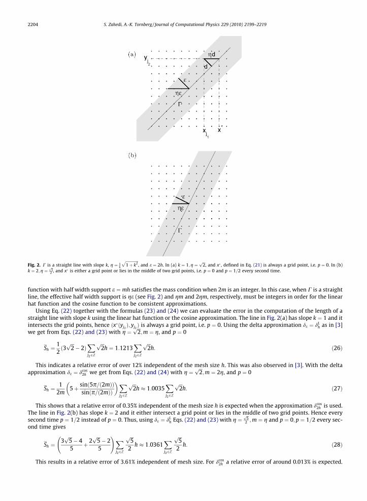
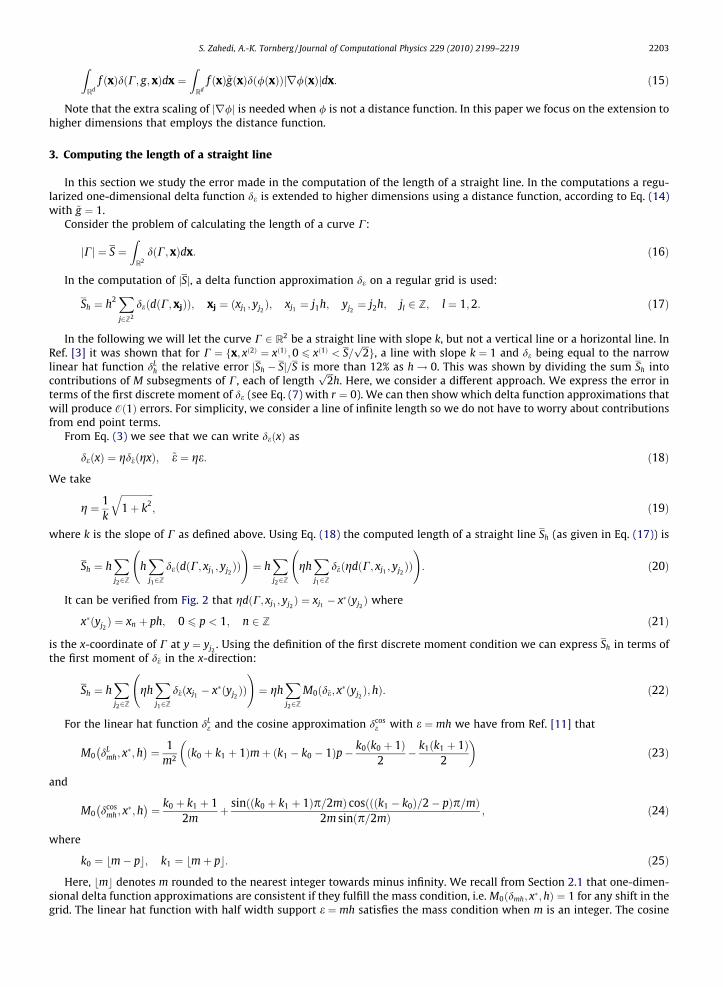
Fig. 2. C is a straight line with slope k, g ¼ 1k

ffiffiffiffiffiffiffiffiffiffiffiffiffiffi1þ k2

p, and e ¼ 2h. In (a) k ¼ 1;g ¼

ffiffiffi2p

, and x� , defined in Eq. (21) is always a grid point, i.e. p ¼ 0. In (b)k ¼ 2;g ¼

ffiffi5p

2 , and x� is either a grid point or lies in the middle of two grid points, i.e. p ¼ 0 and p ¼ 1=2 every second time.


function with half width support e ¼ mh satisfies the mass condition when 2m is an integer. In this case, when C is a straightline, the effective half width support is ge (see Fig. 2) and gm and 2gm, respectively, must be integers in order for the linearhat function and the cosine function to be consistent approximations.

Using Eq. (22) together with the formulas (23) and (24) we can evaluate the error in the computation of the length of astraight line with slope k using the linear hat function or the cosine approximation. The line in Fig. 2(a) has slope k ¼ 1 and itintersects the grid points, hence ðx�ðyj2

Þ; yj2Þ is always a grid point, i.e. p ¼ 0. Using the delta approximation de ¼ dL

h as in [3]we get from Eqs. (22) and (23) with g ¼

ffiffiffi2p

;m ¼ g, and p ¼ 0

Sh ¼12ð3

ffiffiffi2p� 2Þ

Xj22Z

ffiffiffi2p

h ¼ 1:1213Xj22Z

ffiffiffi2p

h: ð26Þ

This indicates a relative error of over 12% independent of the mesh size h. This was also observed in [3]. With the deltaapproximation de ¼ dcos

2h we get from Eqs. (22) and (24) with g ¼ffiffiffi2p

;m ¼ 2g, and p ¼ 0

Sh ¼1

2m5þ sinð5p=ð2mÞÞ

sinðp=ð2mÞÞ

Xj22Z

ffiffiffi2p

h � 1:0035Xj22Z

ffiffiffi2p

h: ð27Þ

This shows that a relative error of 0.35% independent of the mesh size h is expected when the approximation dcos2h is used.

The line in Fig. 2(b) has slope k ¼ 2 and it either intersect a grid point or lies in the middle of two grid points. Hence everysecond time p ¼ 1=2 instead of p ¼ 0. Thus, using de ¼ dL

h Eqs. (22) and (23) with g ¼ffiffi5p

2 ;m ¼ g and p ¼ 0; p ¼ 1=2 every sec-ond time gives

Sh ¼3ffiffiffi5p� 4

5þ 2

ffiffiffi5p� 2

5

!Xj22Z

ffiffiffi5p

2h � 1:0361

Xj22Z

ffiffiffi5p

2h: ð28Þ

This results in a relative error of 3.61% independent of mesh size. For dcos2h a relative error of around 0.013% is expected.


3.1. Numerical validation

In order to validate the results of the previous subsection we consider C being two parallel lines of length L at a normaldistance 2a, joined at both ends by a half circle with radius a. The slope of the lines to the x-axis is k. The length of C isS ¼ 2Lþ 2pa. Contours of the distance function dðC;xÞ when k ¼ 2 are shown in Fig. 3.

In Fig. 4(a) we show the relative error E ¼ jSh � Sj=S where Sh is computed according to Eq. (17) with de ¼ dcos2h and k ¼ 1.

We can clearly see that there is no convergence as h! 0. Eq. (27) indicates that the relative error for the straight lines isaround 0.0035. We can see in the figure that this number is approached when the length of the straight lines is increasedand the radius of the half circles is decreased.

In Fig. 4(b) the slope of the parallel lines is 2 and de ¼ dLh has been used in the computation. There is no convergence. Eq.

(28) indicates that the relative error for the straight lines is around 0.0361. We see in the figure that as the length of thestraight lines is increased or the radius of the half circles is decreased the relative error approaches this number.

3.2. Mass condition reformulated using a Fourier transform

By the use of Poisson’s summation formula

Fig. 3.a ¼ 0:4

aXj2Z

uðajÞ ¼Xj2Z

uðj=aÞ; ð29Þ

the mass condition for a regularized delta function de ¼ 1e uðx=eÞ with e ¼ mh can be related to the Fourier transform of the

function uðnÞ

uðkÞ ¼Z 1

�1uðnÞe�2pikndn; ð30Þ

in the following way:

M0ðdmh; x�;hÞ ¼1m

Xj2Z

uððj� pÞ=mÞ ¼Xj2Z

e�2pijpuðjmÞ: ð31Þ

The linear hat function, uLðnÞ, defined as in Eq. (4), has the Fourier transform

uLðkÞ ¼ sin2ðpkÞp2k2 : ð32Þ

Thus, using Eq. (31) we have

M0ðdLe; x�; hÞ ¼ 1þ

Xj2Z;j – 0

e�2pijp sinðpmjÞpmj

2

; ð33Þ

Here, we have used that uLð0Þ ¼ 1. The second term in Eq. (33) is zero independent of any shift in the grid x� only whensinðpmjÞ ¼ 0 for all j 2 Z; j – 0. Therefore the mass condition is satisfied only for integers m P 1. This result can also be ob-tained using formula (23).

00

0 0.5

0.50.

5

0.5

1

1

1

1

1

1

1.5

1.5

1.5

1.5

1.5

1.5

1.5

2

2

2

2

2

2

2

2

2.5

2.5

2.5

2.5

2.5

2.5

3

3

3

3

3

3

3.5

3.5

3.5

3.5

4

4

4.5

4.5

5

5

−4 −2 0 2 4−4

−3

−2

−1

0

1

2

3

4

Contours of the distance function dðC;xÞ. C is two parallel lines of length L ¼ 4 at a normal distance 2a, joined at both ends by a half circle of radius8=

ffiffiffi5p

. The slope of the lines to the x-axis is 2.

10−3 10−22.7

2.8

2.9

3

3.1

3.2

3.3

3.4

x 10−3

h

Rel

ativ

e er

ror

10−3 10−20.03

0.031

0.032

0.033

0.034

0.035

0.036

h

Rel

ativ

e er

ror

Fig. 4. The relative error E ¼ jSh � Sj=S where C is two parallel lines of length L at a normal distance 2a, joined at both ends by a half circle of radius a. In (a)the slope of the parallel lines is k ¼ 1 and de ¼ dcos

2h is used. Circles: L ¼ 4, a ¼ 0:24ffiffiffi2p

. Stars: L ¼ 6; a ¼ 0:12ffiffiffi2p

. Squares: L ¼ 6; a ¼ 0:03ffiffiffi2p

. The predictedrelative error for the length of lines is around 3:5 10�3. In (b) the slope of the parallel lines is k ¼ 2 and de ¼ dL

h is used. Circles: L ¼ 4; a ¼ 0:48=ffiffiffi5p

. Stars:L ¼ 6; a ¼ 0:12=

ffiffiffi5p

. Squares: L ¼ 6; a ¼ 0:06ffiffiffi2p

. The predicted relative error for the length of lines is around 0.0361.


The cosine approximation ucosðnÞ, defined in Eq. (5), has the Fourier transform

ucosðkÞ ¼sinð2pkÞ

2pk

� �1

1�4k2 ; if k – 1=2;

1=2; if k ¼ 1=2:

(ð34Þ

By the same argument as above we have that the mass condition is satisfied only when sinð2pmjÞ ¼ 0 for all j 2 Z; j – 0and m – 1=2. Therefore, the mass condition is satisfied when m P 1 and 2m is an integer.

In Eq. (22) we needed to evaluate M0ðd~e; x�;hÞ, where ~e ¼ gmh. From Poisson’s summation formula we have

M0ðd~e; x�; hÞ ¼Xj2Z

e�2pijpuðjgmÞ: ð35Þ

Thus, in order to not have Oð1Þ errors in the computation of the length of a straight line, m in e ¼ mh must be chosen suchthat gm P 1 is an integer when de ¼ dL

e and gm P 1, 2gm is an integer when de ¼ dcose .

Remark. The regularized one-dimensional delta functions were in this section extended using the distance function. Ifinstead a non-distance function /ðxÞ is used e must be chosen differently in order to avoid Oð1Þ errors. This is due to the factthat /ðxÞ does not give the physical distance, and hence a different scaling is needed.

Assume that uðkÞ has compact support on (�1, 1) and that uð0Þ ¼ 1. Then, by Eq. (35), for all m P 1=g, the mass condi-tion is satisfied. When /ðxÞ is a distance function we have that g P 1. This arises from the fact that the distance from C mea-sured along a grid line is always larger or equal to the closest distance to C, which is given by the distance function, see Fig. 2.When g P 1 then for all m P 1, there is no Oð1Þ error. If /ðxÞ is not a distance function and jr/j > 1, a harder restriction onm is needed.

In the next section, we introduce a class of one-dimensional delta functions for which the uðkÞ functions have compactsupport. We will see that this type of delta function approximations will satisfy the discrete moment conditions for a widerange of dilations.

4. Approximations with compact support in Fourier space

In the last section we saw that the linear hat function dLe and the cosine approximation dcos

e with e ¼ mh are consistentapproximations in one dimension only for a discrete set of m-values. Therefore they can lead to inconsistent approximationsin higher dimensions. However, it is possible to construct delta function approximations that obey the mass condition for awide range of dilations. We start by stating a theorem

Theorem 4.1. Assume a regular grid in one dimension with grid points xj ¼ jh; j 2 Z and let x� ¼ xn þ ph where 0 6 p < 1 andn 2 Z. Consider a delta function approximation de ¼ 1

e uðx=eÞ with e ¼ mh where

uðnÞ ¼Z 1

�1uðkÞe2pikndk ð36Þ

and the Fourier transform of u

uðkÞ ¼Z 1

�1uðnÞe�2pikndn: ð37Þ

If uðkÞ has compact support on ð�b; bÞ and


@ruðkÞ@kr

��k¼0¼

1; for r ¼ 0;0; for 1 6 r < q:

�ð38Þ

Then for all m P b the delta function approximation de satisfies q discrete moment conditions.

The discrete moment conditions are important for the accuracy of the one-dimensional delta function approximation, seeProposition 2.1. The conditions in Eq. (38) in the theorem are equivalent to the continuous moment conditions, i.e.

@ruðkÞ@kr

��k¼0¼

1; for r ¼ 0;0; for 1 6 r < q

�()

Z 1

�1uðxÞxrdx ¼

1; for r ¼ 0;0; for 1 6 r < q:

�ð39Þ

The continuous moment conditions will be important as we consider the analytical error in higher dimensions.Proof of Theorem 4.1 There is no restriction in taking n ¼ 0, such that x� ¼ ph, with 0 6 p < 1. Let fr;eðxÞ ¼ 1

e uðx=eÞxr . Wehave

Mrðde; x�;hÞ ¼ hXj2Z

deðxj � x�Þðxj � x�Þr ¼ hXj2Z

1euððxj � x�Þ=eÞðxj � x�Þr ¼ h

Xj2Z

fr;eððj� pÞhÞ: ð40Þ

Since the Fourier transform of fr;eðxÞ is

f r;eðkÞ ¼1

ð�2piÞr@r

@kr uðekÞ ð41Þ

and the Fourier transform of fr;eðx� x�Þ is e�2pikx� f r;eðkÞ we have from Poisson’s summation formula Eq. (29) that

Mrðde; x�;hÞ ¼Xk2Z

e�2pikp 1ð�2piÞr

@r

@kr uðek=hÞ: ð42Þ

with e ¼ mh we get

Mrðde; x�;hÞ ¼1

ð�2piÞr@ruðmkÞ@kr

��k¼0þ 1ð�2piÞr

Xk2Z;k – 0

e�2pikp @r

@kr uðmkÞ: ð43Þ

If uðkÞ has compact support in ð�b; bÞ the second term in the above equation vanishes for all m P b. Hence if the condi-tion in Eq. (38) is satisfied for r ¼ 0;1; . . . ; q� 1 then de ¼ 1

e uðx=eÞ satisfies q discrete moment conditions. h

An example of a delta function approximation with the function uðkÞ having compact support is the delta function intro-duced in Ref. [11]

dTEe ðxÞ ¼

1euTEðx=eÞ ð44Þ

with

uTEðnÞ ¼Z 1

�1uTEðkÞe2pikndk; uTEðkÞ ¼ e

1db2 e

1dðk2�b2Þ if jkj < b;

0 if jkjP b;

(ð45Þ

d ¼ 0:1 and b ¼ 1. Note that

uTEð0Þ ¼ 1;@uTEðkÞ@k

��k¼0¼ 0;

@2uTEðkÞ@k2

��k¼0

¼ �2db4 – 0: ð46Þ

Hence from Theorem 4.1 we have that dTEmhðxÞ is of moment order 2 for all m P 1. Thus, it is possible to construct one-

dimensional delta function approximations that obey the discrete moment conditions for a wide range of dilations. Thesedelta function approximations will not have compact support since they have compact support in Fourier space. However,if an approximation is decaying rapidly it can in practice be truncated.

It is computationally demanding to evaluate the approximation from its Fourier transform. Therefore, we would like tohave an explicit expression for the approximation. In the following we give explicit expressions for two delta functionapproximations which have Fourier transforms that decay rapidly. Theorem 4.1 can then be used to find m-values for whichdmhðxÞ satisfies the discrete moment conditions within a given error tolerance.

4.1. The derivative of the Fermi–Dirac function

Define a delta approximation as the derivative of the Fermi–Dirac or the sigmoid function

dFDe ðxÞ ¼ @x

11þ e�x=e ¼

1e

e�x=e

ð1þ e�x=eÞ2: ð47Þ

Let then dFDe ðxÞ ¼ 1

e uFDðx=eÞ, where

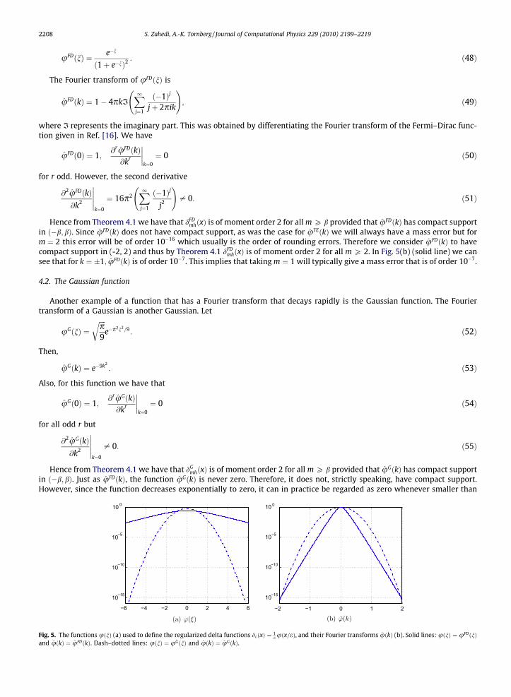
Fig. 5.and uð


uFDðnÞ ¼ e�n

ð1þ e�nÞ2: ð48Þ

The Fourier transform of uFDðnÞ is

uFDðkÞ ¼ 1� 4pkIX1j¼1

ð�1Þj

jþ 2pik

!; ð49Þ

where I represents the imaginary part. This was obtained by differentiating the Fourier transform of the Fermi–Dirac func-tion given in Ref. [16]. We have

uFDð0Þ ¼ 1;@ruFDðkÞ@kr

��k¼0¼ 0 ð50Þ

for r odd. However, the second derivative

@2uFDðkÞ@k2

��k¼0

¼ 16p2X1j¼1

ð�1Þj

j2

!– 0: ð51Þ

Hence from Theorem 4.1 we have that dFDmhðxÞ is of moment order 2 for all m P b provided that uFDðkÞ has compact support

in ð�b; bÞ. Since uFDðkÞ does not have compact support, as was the case for uTEðkÞ we will always have a mass error but form ¼ 2 this error will be of order 10�16 which usually is the order of rounding errors. Therefore we consider uFDðkÞ to havecompact support in (-2, 2) and thus by Theorem 4.1 dFD

mhðxÞ is of moment order 2 for all m P 2. In Fig. 5(b) (solid line) we cansee that for k ¼ 1; uFDðkÞ is of order 10�7. This implies that taking m ¼ 1 will typically give a mass error that is of order 10�7.

4.2. The Gaussian function

Another example of a function that has a Fourier transform that decays rapidly is the Gaussian function. The Fouriertransform of a Gaussian is another Gaussian. Let

uGðnÞ ¼ffiffiffiffip9

re�p2n2=9: ð52Þ

Then,

uGðkÞ ¼ e�9k2: ð53Þ

Also, for this function we have that

uGð0Þ ¼ 1;@ruGðkÞ@kr

��k¼0¼ 0 ð54Þ

for all odd r but

@2uGðkÞ@k2

��k¼0

– 0: ð55Þ

Hence from Theorem 4.1 we have that dGmhðxÞ is of moment order 2 for all m P b provided that uGðkÞ has compact support

in ð�b; bÞ. Just as uFDðkÞ, the function uGðkÞ is never zero. Therefore, it does not, strictly speaking, have compact support.However, since the function decreases exponentially to zero, it can in practice be regarded as zero whenever smaller than

−6 −4 −2 0 2 4 6

10−15

10−10

10−5

10 0

−2 −1 0 1 2

10−15

10−10

10−5

10 0

The functions uðnÞ (a) used to define the regularized delta functions deðxÞ ¼ 1e uðx=eÞ, and their Fourier transforms uðkÞ (b). Solid lines: uðnÞ ¼ uFDðnÞ

kÞ ¼ uFDðkÞ. Dash–dotted lines: uðnÞ ¼ uGðnÞ and uðkÞ ¼ uGðkÞ.


some tolerance. In Fig. 5(b) we see the function uGðkÞ (dash–dotted line). For k ¼ 1; uGðkÞ is of order 10�5 and for k ¼ 2 itis of order 10�16 just as uFDðkÞ. With an error tolerance of 10�16 we consider uGðkÞ to be of moment order 2 for all m P 2. Wecan see from Fig. 5(a) that the support of uGðnÞ is much smaller than uFDðnÞ. Since, in practical computations, a narrow sup-port of uðnÞ is desired the Gaussian approximation seems to be preferable.

In the next section we state and prove theorems about the error when the distance function is used to extend the one-dimensional delta approximations to higher dimensions.

5. Error analysis

Let X be the domain of integration. We assume throughout this section that the approximation deðdðC;xÞÞ has compactsupport in

Xx ¼ fx : jdðC;xÞj 6 xg; ð56Þ

where dðC;xÞ is the signed distance function and x is small. We want to integrate

IC;F ¼Z

XdðdðC; xÞÞFðxÞdx: ð57Þ

The total error in the integration of the function dðdðC;xÞÞFðxÞ approximated by deðdðC;xÞÞFðxÞ is

Etot;FðdeÞ ¼Z

XdðdðC;xÞÞFðxÞdx� quadðdeðdðC;xÞÞFðxÞÞ; ð58Þ

where quad denotes the quadrature rule used to approximate the integral. The quadrature rule we consider is the trapezoidalrule. We split the total error into two parts: the analytical error made when replacing the integrand with its approximation

Ex;FðdeÞ ¼Z

Xx

dðdðC;xÞÞFðxÞdx�Z

Xx

deðdðC; xÞÞFðxÞdx ð59Þ

and the numerical error made in the integration of this approximation using the trapezoidal rule

Equad;FðdeÞ ¼Z

Xx

deðdðC;xÞÞFðxÞdx� quadðdeðdðC; xÞÞFðxÞÞ: ð60Þ

5.1. Analytical error

Definition 5.1. A function de with compact support in ½�x;x� satisfies a continuous moment conditions if
Z x
�xdeðtÞtrdt ¼

1; if r ¼ 0;0; if 1 6 r < a:

�ð61Þ

We now state two theorems for the analytical error. The first theorem provides an expression for the analytical error intwo dimensions, and the second theorem in three dimensions.

Theorem 5.1. Let de be a continuous function with support in ½�x;x�;x ¼ pe that satisfies a continuous moment conditions, seeDefinition 5.1. Assume that C, the zero level set of dðC;xÞ, is a curve in R2 of class C2 that can be parametrized byC ¼ ðxðsÞ; yðsÞÞ; x; y 2 C2½s1; s2� with the curvature jðsÞ defined by

jðsÞ ¼ x0ðsÞy00ðsÞ � x00ðsÞy0ðsÞqðsÞ3

; qðsÞ ¼ffiffiffiffiffiffiffiffiffiffiffiffiffiffiffiffiffiffiffiffiffiffiffiffiffiffiffiffiffix0ðsÞ2 þ y0ðsÞ2

q– 0: ð62Þ

Assume also that

x maxsjjðsÞj < 1; ð63Þ

and that FðxÞ is a smooth function. Then, the analytical error for the integration of dðdðC;xÞÞFðxÞ made when replacing dðdðC;xÞÞby deðdðC;xÞÞ is given by

Ex;FðdeÞ ¼ �eaCa;F

Z p

�puðnÞnadnþ Oðeaþ1Þ; ð64Þ

with

Ca;F ¼1a!

Z s2

s1

qðsÞfatðs;0Þds� 1ða� 1Þ!

Z s2

s1

qðsÞjðsÞfða�1Þtðs;0Þds: ð65Þ

A proof of this theorem for p ¼ 1 is given in Ref. [12] but a generalization is straightforward. The parametrization ofC ¼ ðxðsÞ; yðsÞÞ and the normal vector of the curve defined by


n ¼ ð�y0ðsÞ; x0ðsÞÞqðsÞ ð66Þ

are used to parametrize the integration domain Xx. Introducing the parametrization Xðs; tÞ ¼ xðsÞ þ tn1ðsÞ;Yðs; tÞ ¼ yðsÞ þ tn2ðsÞ. The integration can be performed over ½s1; s2� � ½�x;x� when the condition in Eq. (63) is fulfilled.The function f in Eq. (65) is defined by

f ðs; tÞ ¼ FðXðs; tÞ; Yðs; tÞÞ: ð67Þ

Theorem 5.2. Let de be a continuous function with support in ½�x;x�;x ¼ pe that satisfies a continuous moment conditions, seeDefinition 5.1. Assume that C, the zero level set of dðC;xÞ, is a 2-manifold in R3 of class C2. Suppose thatPjðr; sÞ ¼ ðxðr; sÞ; yðr; sÞ; zðr; sÞÞ : ðr1; r2Þ � ðs1; s2Þ ! Vj is a coordinate patch on C of class C2 and C is covered by the disjointunion of the open sets V1; . . . ;Vl and a set of measure zero in C. Let j1 and j2 be the principal curvatures of C on Vj. Assume alsothat

x maxðmaxr;sjj1ðr; sÞj;max

r;sjj2ðr; sÞjÞ < 1; qðr; sÞ ¼ kPj

r � Pjsk – 0; ð68Þ

and that FðxÞ is a smooth function. Then, the analytical error for the integration of dðdðC;xÞÞFðxÞ made when replacing dðdðC;xÞÞby deðdðC;xÞÞ is given by

Ex;FðdeÞ ¼ �eaZ p

�puðnÞnadn

Xl

j¼1

Cja;F þ Oðeaþ1Þ; ð69Þ

with

Cj1;F ¼

Z r2

r1

Z s2

s1

ftðr; s;0Þqðr; sÞdsdr �Z r2

r1

Z s2

s1

f ðr; s; 0Þqðr; sÞðj1ðr; sÞ þ j2ðr; sÞÞdsdr ð70Þ

and for a P 2

Cja;F ¼

1a!

Z r2

r1

Z s2

s1

qðr; sÞfatðr; s;0Þdsdr � 1ða� 1Þ!

Z r2

r1

Z s2

s1

qðr; sÞðj1ðr; sÞ þ j2ðr; sÞÞfða�1Þtðr; s;0Þdsdr

þ 1ða� 2Þ!

Z r2

r1

Z s2

s1

qðr; sÞðj1ðr; sÞj2ðr; sÞÞfða�2Þtðr; s; 0Þdsdr: ð71Þ

A proof can be found in the Appendix A. In order to perform the integration over Xx we parametrize this region using thelocal parametrization of C and the normal vectors defined as

n ¼ ðn1; n2;n3Þ ¼ 1qðr; sÞ ðP

jr � Pj

sÞ: ð72Þ

Introducing the parametrization Xjðr; s; tÞ ¼ xðr; sÞ þ tn1ðr; sÞ;Yjðr; s; tÞ ¼ yðr; sÞ þ tn2ðr; sÞ, and Zjðr; s; tÞ ¼ zðr; sÞ þ tn3ðr; sÞwe can cover the domain Xx by disjoint union of open sets M1; . . . ;Ml and a set of measure zero in Xx, where

Mj ¼ fðx; y; zÞ : x ¼ Xjðr; s; tÞ; y ¼ Yjðr; s; tÞ; z ¼ Zjðr; s; tÞ; r 2 ðr1; r2Þ; s 2 ðs1; s2Þ; t 2 ½�x;x�g: ð73Þ

The condition in Eq. (68) guarantees that this parametrization is non-singular. The integration can then be performed over½r1; r2� � ½s1; s2� � ½�x;x�. For x small one can Taylor expand

f ðr; s; tÞ ¼ FðXjðr; s; tÞ; Yjðr; s; tÞ; Zjðr; s; tÞÞ ð74Þ

around ðr; s;0Þ and express the analytical error in terms of the continuous moments of the function de.In the next section we analyze the numerical error made using the trapezoidal rule for integration.

5.2. Numerical error

The following theorem gives the error of the trapezoidal rule in one dimension.

Theorem 5.3. Let

xn ¼ aþ nh; n ¼ 0; . . . N; h ¼ b� aN

ð75Þ

be a decomposition of the interval ½a; b� and Thða; b;h;wÞ be the trapezoidal sum

Thða; b;h;wÞ ¼ hXN

n¼0

wnwðxnÞ; ð76Þ


where

wn ¼1=2; for n ¼ 0; and n ¼ N;

1; otherwise:

�ð77Þ

Assume that wðxÞ 2 C2rþ2ða; bÞ. Then

Th �Z b

awðxÞdx ¼ RTða; b;h;wðxÞÞ ð78Þ

with

RTða; b;h;wðxÞÞ ¼Xr

k¼1

B2kh2k

ð2kÞ! w2k�1ðxÞ��bx¼aþ R2rþ2ða; b;h;wÞ; ð79Þ

where Bj are the Bernoulli numbers and R2rþ2ða; b;h;wÞ is Oðh2rþ2Þ.

For a proof see Ref. [17, p. 298]. Note that when the function wðxÞ 2 C1 for x 2 R and w has ½a; b� as an interval of period-icity, then

wðkÞðbÞ ¼ wðkÞðaÞ; k ¼ 0;1;2; . . . : ð80Þ

Hence,

jRTða; b; h;wÞj ¼ Oðh2rþ2Þ ð81Þ

for arbitrary r. Therefore, we have that for periodic infinite differentiable functions the trapezoidal error tends to zero fasterthan any power of h, as h! 0. This is referred to as superconvergence. In Ref. [18] another proof is given. It is shown by usingthe Poisson summation formula that the error

RT ¼ hXN

n¼0

wnwðxnÞ �Z b

awðxÞdx: ð82Þ

decreases as wð1=hÞ, with

wðkÞ ¼Z 1

�1wðxÞe�2pikxdx: ð83Þ

If w 2 Cr½R� and periodic, then wð1=hÞ ¼ OðhrÞ, as h! 0. Thus, for w 2 C1½R� the trapezoidal rule converges faster than anypower of h.

In higher dimensions we use the notion of a product rule. For simplicity we do the analysis here in two dimensions. Theanalysis in three dimensions is similar. Let X ¼ ½a; b� � ½c; d�, and wðx; yÞ 2 C2rþ2ðXÞ. Introduce a uniform grid

xj ¼ aþ jhx; j ¼ 0; . . . M; hx ¼b� a

M; yn ¼ c þ nhy; n ¼ 0; . . . N; hy ¼

d� cN

: ð84Þ

Denote by Q the quadrature scheme obtained by using the trapezoidal rule in both x and y directions with step size hx andhy. We can write

I ¼Z Z

Xwðx; yÞdxdy ¼

Z d

cgðyÞdy; ð85Þ

where

gðyÞ ¼Z b

awðx; yÞdx: ð86Þ

Using the trapezoidal rule to integrate in the y-variable (see, Eqs. (76) and (77)) gives

I ¼ hy

XN

n¼0

wn

Z b

awðx; ynÞdxþ RTðc; d;hy; gðyÞÞ; ð87Þ

where RT is the quadrature error. Using also the trapezoidal method in the x-direction with step size hx yields

I ¼ hy

XN

n¼0

wn hx

XM

j¼0

wjwðxj; ynÞ þ RTða; b;hx;wðx; ynÞÞ !

þ RTðc;d; hy; gðyÞÞ: ð88Þ

Simplifying the expression we get


I ¼ hyhx

XN

n¼0

XM

j¼0

wnwjwðxj; ynÞ þXN

n¼0

hywnRTða; b;hx;wðx; ynÞÞ þ RT c;d;hy;

Z b

awðx; yÞdx

!: ð89Þ

Hence

I � hyhx

XN

n¼0

XM

j¼0

wnwjwðxj; ynÞ��

�� 6 ðd� cÞmaxyn

RTða; b;hx;wðx; ynÞÞj j þ ðb� aÞmaxx2½a;b�

RT c;d;hy;wðx; yÞ� �� ; ð90Þ

and we see that the convergence results from one dimension extend to two dimensions. Thus, the superconvergence of thetrapezoidal rule also applies in two dimensions. We are now able to formulate the following theorem.

Theorem 5.4. Let X ¼ ½a; b� � ½c; d�, and Q be the quadrature scheme obtained by using the trapezoidal rule in both x and ydirections with step size hx and hy. Suppose de has compact support in ½�x;x� and Xx � X where

Xx ¼ fx : jdðC;xÞj 6 xg: ð91Þ

Suppose further that deðdðC;xÞÞFðxÞ 2 C1ðXÞ. Then the numerical error

EQ ;FðdeÞ ¼Z

XdeðdðC;xÞÞFðxÞdx� QðdeðdðC;xÞÞFðxÞÞ

�� ð92Þ

decreases faster than any power of h ¼ maxðhx;hyÞ.

When de has compact support in ½�x;x� the approximation deðdðC;xÞÞ has compact support in Xx. As long asXx � X; deðdðC;xÞÞ is a periodic function on X. Since the integrand is C1ðXÞ the superconvergence of the trapezoidal rulegives the result of the theorem.

The same result also holds in three dimensions.

5.3. Practical considerations

The theorems in the previous section are applicable to delta function approximations with compact support in ½�x;x�.The delta function approximations presented in Section 4 are infinitely differentiable and satisfy two moment conditions butdo not have compact support. In practice, we will truncate the delta function approximations presented in Section 4 and setthem to zero outside some ½�x;x� interval. This is motivated by the fact that the delta function approximations de in ques-tion decay exponentially fast. The truncation results in an approximation error. In the following, we comment on the errorwe make by truncating the tail of dFD

e and dGe and discuss how the theorems in the previous section can be used.

Denote the truncated delta function approximation by

dxe ðtÞ ¼

deðtÞ; for t in ½�x;x�;0; otherwise;

�ð93Þ

where deðtÞ is one of the one-dimensional delta function approximations presented in Section 4 and x is the half width sup-port of the truncated delta function.

In two and three dimensions, we split the total error in the integration of the function dðdðC;xÞÞFðxÞ approximated bydxe ðdðC;xÞÞFðxÞ into two parts: the analytical error Ex;Fðdx

e Þ defined in Eq. (59) and the numerical error Equad;Fðdxe Þ defined

in Eq. (60). The analytical error in two dimensions is given by Theorem 5.1 and in three dimensions by Theorem 5.2. Thiserror depends on the number of continuous moment conditions the delta function approximation satisfies. All the delta func-tion approximations de in Section 4 satisfy two continuous moment conditions, see Eq. (39). By truncating these delta func-tion approximations we make an approximation error and the continuous moment conditions are only satisfied to a certainlevel of accuracy depending on the truncation parameter x.

In the following, we estimate the error we make by truncating the tail of de. In two dimensions the analytical error for thetruncated approximation dx

e is

Ex;Fðdxe Þ ¼ 1�

Z x

�xdxe ðtÞdt

Z s2

s1

qðsÞf ðs;0Þds� C1;F

Z x

�xdxe ðtÞtdt þ Oðe2Þ; ð94Þ

where C1;F ; qðsÞ, and f ðs; tÞ are all defined in Theorem 5.1. Note that the only difference in three dimensions are the constantsin front of the one-dimensional continuous moment conditions, see Theorem 5.2.

Since both dFDe and dG

e are even functions we have that
Z �x
�1deðtÞtdt þ

Z 1

xdeðtÞtdt ¼ 0: ð95Þ

From the definition of dxe , Eq. (93) and since both dFD

e and dGe satisfy the second continuous moment condition, i.e.
Z 1
�1deðtÞtdt ¼

Z x

�xdeðtÞtdt þ

Z �x

�1deðtÞtdt þ

Z 1

xdeðtÞtdt ¼ 0; ð96Þ


the compactly supported delta function approximations also satisfy the second moment condition and hence the secondterm in Eq. (94) is zero. To estimate the first term in Eq. (94) we need to estimate

Fig. 6.toleranwas useof wheraround

I1 ¼Z 1

xdeðtÞf ðtÞdt ð97Þ

and

I2 ¼Z x

�1deðtÞf ðtÞdt: ð98Þ

For de ¼ dFDe ðtÞ we have

jIFD1 þ IFD

2 j ¼2

1þ ex=e ð99Þ

and for de ¼ dGe ðtÞ

jIG1 þ IG

2 j ¼ 1� erfpx3e

� �; ð100Þ

where erf is the error function defined by

erfðxÞ ¼ 2ffiffiffiffipp

Z x

0e�t2

dt: ð101Þ

Thus, given a tolerance one can choose x=e such that jI1 þ I2j is below the given tolerance. Then, the analytical error isOðe2Þ down to the given tolerance.

The analysis of the numerical error in two and three dimensions presented in Section 5.2 is based on the superconver-gence of the trapezoidal rule for periodic infinitely differentiable functions. By truncating the delta function approximationspresented in Section 4 we make an approximation error and a mismatch in the odd derivatives at x, i.e.u2k�1ðxÞ – u2k�1ð�xÞ results in an error, see Theorem 5.3. However, if the function u is very small when truncated we ex-pect the error in the trapezoidal rule to be small.

The total error is hence a sum of the analytical and the numerical error. We suggest here a way to select e and the halfwidth support x so that the delta function approximations with compact support are second-order accurate down to a spec-ified error tolerance. We have seen in numerical experiments that choosing x and e according to this algorithm gives a totalerror below the given tolerance. Given a tolerance C, appropriate values for e and x can be determined by the followingsteps:

1. choose the smallest b such that uðbÞ < C,2. let e ¼ mh and take m ¼ b, then3. for this e choose x such that4. deðxÞ 6 C.

In the first step we want to get a one-dimensional delta function approximation dmh that satisfies two discrete momentconditions down to the specified error tolerance C for all m P b. In the second step we choose the smallest such m and in thethird step we truncate the delta function within the same accuracy. In Figs. 6 and 7 we show the chosen m and x=h for

10−15 10−10 10−5

0.6

0.8

1

1.2

1.4

1.6

1.8

2

2.2

Error tolerance

m

10−15 10−10 10−52

4

6

8

10

12

14

Error tolerance

ω /

h

For the delta function dGmh we show in (a) m as a function of error tolerance. We show the smallest m such that uGðmÞ is below the given error

ce. In (b) we show the half width support of dGmh divided by h when m from (a) is used. The support is computed with the same error tolerance that

d to find the appropriate m-value. This calculation was made for two different values of h;h ¼ 10�6 (stars) and h ¼ 10�2 (squares) and gives an ideae the delta function approximation can be truncated. For a tolerance of 10�6 the optimal m is, for example, around 1.25 and the half width support is6h, while for a requested tolerance of 10�16 ;m � 2 and the half width support is around 14h.

10−15 10−10 10−5

0.6

0.8

1

1.2

1.4

1.6

1.8

2

2.2

Error tolerance

m

10−15 10−10 10−5 1000

20

40

60

80

100

Error tolerance

ω /

h

Fig. 7. The delta function dFDmh is used. This figure should be compared with Fig. 6. In (a) we show the smallest m such that uGðmÞ is below the given error

tolerance. In (b) we show the half width support divided by h of dFDmh when m from (a) is used. The support is computed with the same error tolerance that

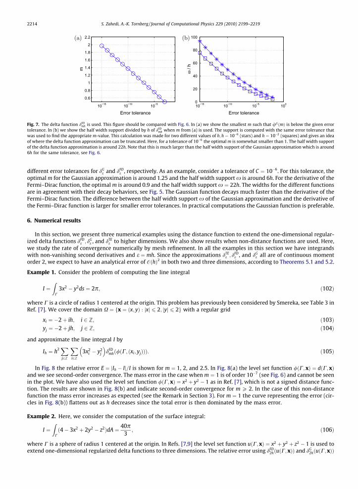
was used to find the appropriate m-value. This calculation was made for two different values of h;h ¼ 10�6 (stars) and h ¼ 10�2 (squares) and gives an ideaof where the delta function approximation can be truncated. Here, for a tolerance of 10�6 the optimal m is somewhat smaller than 1. The half width supportof the delta function approximation is around 22h. Note that this is much larger than the half width support of the Gaussian approximation which is around6h for the same tolerance, see Fig. 6.


different error tolerances for dGe and dFD

e , respectively. As an example, consider a tolerance of C ¼ 10�6. For this tolerance, theoptimal m for the Gaussian approximation is around 1.25 and the half width support x is around 6h. For the derivative of theFermi–Dirac function, the optimal m is around 0.9 and the half width support x ¼ 22h. The widths for the different functionsare in agreement with their decay behaviors, see Fig. 5. The Gaussian function decays much faster than the derivative of theFermi–Dirac function. The difference between the half width support x of the Gaussian approximation and the derivative ofthe Fermi–Dirac function is larger for smaller error tolerances. In practical computations the Gaussian function is preferable.

6. Numerical results

In this section, we present three numerical examples using the distance function to extend the one-dimensional regular-ized delta functions dFD

e ; dGe , and dTE

e to higher dimensions. We also show results when non-distance functions are used. Here,we study the rate of convergence numerically by mesh refinement. In all the examples in this section we have integrandswith non-vanishing second derivatives and e ¼ mh. Since the approximations dTE

e ; dFDe , and dG

e all are of continuous momentorder 2, we expect to have an analytical error of OðhÞ2 in both two and three dimensions, according to Theorems 5.1 and 5.2.

Example 1. Consider the problem of computing the line integral

I ¼Z

C3x2 � y2ds ¼ 2p; ð102Þ

where C is a circle of radius 1 centered at the origin. This problem has previously been considered by Smereka, see Table 3 inRef. [7]. We cover the domain X ¼ fx ¼ ðx; yÞ : jxj 6 2; jyj 6 2g with a regular grid

xi ¼ �2þ ih; i 2 Z; ð103Þyj ¼ �2þ jh; j 2 Z; ð104Þ

and approximate the line integral I by

Ih ¼ h2Xj2Z

Xi2Z

3x2i � y2

j

� �dFD

mhð/ðC; ðxi; yjÞÞÞ: ð105Þ

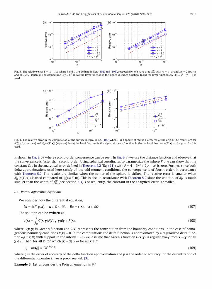
In Fig. 8 the relative error E ¼ jIh � Ij=I is shown for m ¼ 1, 2, and 2.5. In Fig. 8(a) the level set function /ðC;xÞ ¼ dðC; xÞand we see second-order convergence. The mass error in the case when m ¼ 1 is of order 10�7 (see Fig. 6) and cannot be seenin the plot. We have also used the level set function /ðC;xÞ ¼ x2 þ y2 � 1 as in Ref. [7], which is not a signed distance func-tion. The results are shown in Fig. 8(b) and indicate second-order convergence for m P 2. In the case of this non-distancefunction the mass error increases as expected (see the Remark in Section 3). For m ¼ 1 the curve representing the error (cir-cles in Fig. 8(b)) flattens out as h decreases since the total error is then dominated by the mass error.

Example 2. Here, we consider the computation of the surface integral:

I ¼Z

Cð4� 3x2 þ 2y2 � z2ÞdA ¼ 40p

3; ð106Þ

where C is a sphere of radius 1 centered at the origin. In Refs. [7,9] the level set function uðC;xÞ ¼ x2 þ y2 þ z2 � 1 is used toextend one-dimensional regularized delta functions to three dimensions. The relative error using dFD

2hðuðC;xÞÞ and dG2hðuðC;xÞÞ

10−3 10−2 −110−6

10−4

10−2

100

h

Rel

ativ

e er

ror

m = 1m = 2m = 2.5y = h2

10−3 10−2 10−110−6

10−4

10−2

100

h

Rel

ativ

e er

ror

m = 1m = 2m = 2.5y = h2

Fig. 8. The relative error E ¼ jIh � Ij=I where I and Ih are defined in Eqs. (102) and (105), respectively. We have used dFDmh with m ¼ 1 (circles), m ¼ 2 (stars),

and m ¼ 2:5 (squares). The dashed line is y ¼ h2. In (a) the level function is the signed distance function. In (b) the level function /ðC;xÞ ¼ x2 þ y2 � 1 isused.

10−2 10−110−8

10−6

10−4

10−2

100

h

Rel

ativ

e er

ror

δ2hFD

δ2hG,9

y = h4

10−2 10−110−8

10−6

10−4

10−2

100

h

Rel

ativ

e er

ror

δ2hFD

δ2hG,9

y = h2

Fig. 9. The relative error in the computation of the surface integral in Eq. (106) when C is a sphere of radius 1 centered at the origin. The results are fordFD

2hðuðC;xÞÞ (stars) and dG2hðuðC;xÞÞ (squares). In (a) the level function is the signed distance function. In (b) the level function uðC;xÞ ¼ x2 þ y2 þ z2 � 1 is

used.


is shown in Fig. 9(b), where second-order convergence can be seen. In Fig. 9(a) we use the distance function and observe thatthe convergence is faster than second-order. Using spherical coordinates to parametrize the sphere C one can show that theconstant C2;F in the analytical error defined in Theorem 5.2 (Eq. (71)) with F ¼ 4� 3x2 þ 2y2 � z2 is zero. Further, since bothdelta approximations used here satisfy all the odd moment conditions, the convergence is of fourth-order, in accordancewith Theorem 5.2. The results are similar when the center of the sphere is shifted. The relative error is smaller whendG

2hðuðC;xÞÞ is used compared to dFD2hðuðC;xÞÞ. This is also in accordance with Theorem 5.2 since the width x of dG

2h is muchsmaller than the width of dFD

2h (see Section 5.3). Consequently, the constant in the analytical error is smaller.

6.1. Partial differential equations

We consider now the differential equation,

Lu ¼ dðC; g;xÞ; x 2 X � Rd; Bu ¼ rðxÞ; x 2 @X: ð107Þ

The solution can be written as

uðxÞ ¼Z

XGðx; yÞdðC; g; yÞdy þ RðxÞ; ð108Þ

where Gðx; yÞ is Green’s function and RðxÞ represents the contribution from the boundary conditions. In the case of homo-geneous boundary conditions RðxÞ ¼ 0. In the computations the delta function is approximated by a regularized delta func-tion deðC; g;xÞ with support in the interval ½�x;x�. Assume that Green’s function Gðx; yÞ is regular away from x ¼ y for ally 2 C. Then, for all xj for which jxj � xj > x for all x 2 C,

juj � uðxjÞj 6 Chminðp;qÞ; ð109Þ

where q is the order of accuracy of the delta function approximation and p is the order of accuracy for the discretization ofthe differential operator L. For a proof see Ref. [3].

Example 3. Let us consider the Poisson equation in R2

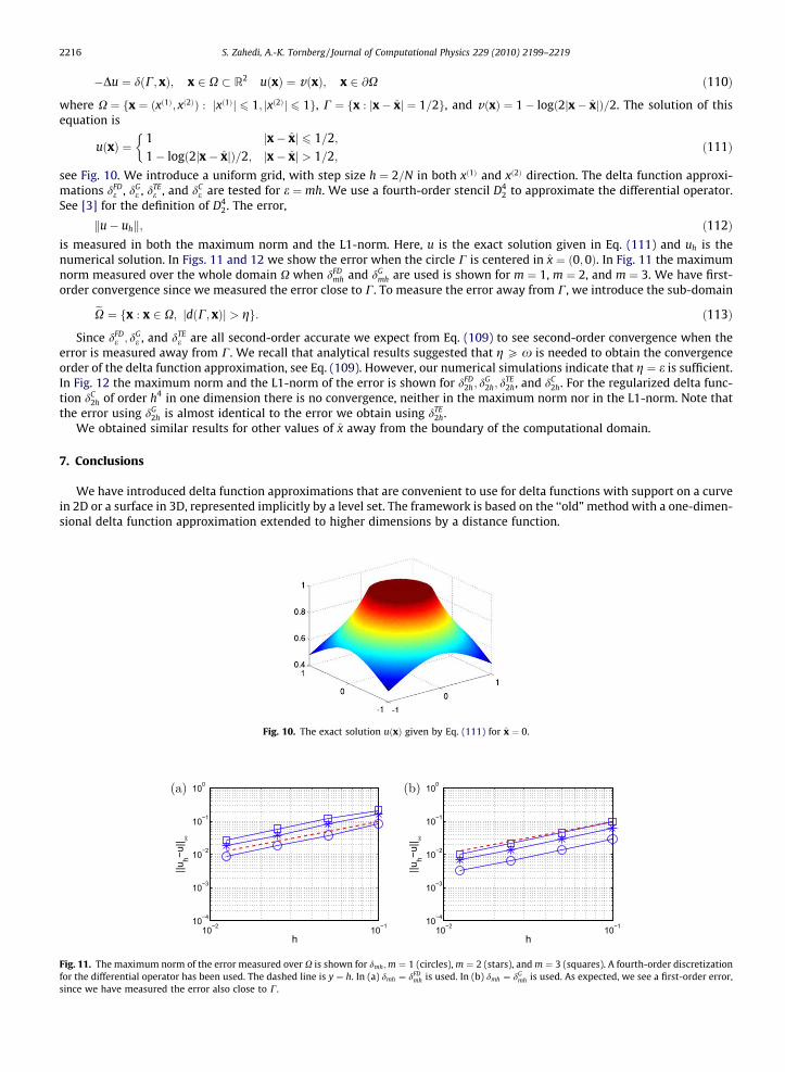
Fig. 11.for thesince w


�Du ¼ dðC;xÞ; x 2 X � R2 uðxÞ ¼ vðxÞ; x 2 @X ð110Þ

where X ¼ fx ¼ ðxð1Þ; xð2ÞÞ : jxð1Þj 6 1; jxð2Þj 6 1g, C ¼ fx : jx� xj ¼ 1=2g, and vðxÞ ¼ 1� logð2jx� xjÞ=2. The solution of thisequation is

uðxÞ ¼1 jx� xj 6 1=2;1� logð2jx� xjÞ=2; jx� xj > 1=2;

�ð111Þ

see Fig. 10. We introduce a uniform grid, with step size h ¼ 2=N in both xð1Þ and xð2Þ direction. The delta function approxi-mations dFD

e , dGe , dTE

e , and dCe are tested for e ¼ mh. We use a fourth-order stencil D4

2 to approximate the differential operator.See [3] for the definition of D4

2. The error,

ku� uhk; ð112Þ
is measured in both the maximum norm and the L1-norm. Here, u is the exact solution given in Eq. (111) and uh is thenumerical solution. In Figs. 11 and 12 we show the error when the circle C is centered in x ¼ ð0;0Þ. In Fig. 11 the maximumnorm measured over the whole domain X when dFD
mh and dGmh are used is shown for m ¼ 1, m ¼ 2, and m ¼ 3. We have first-

order convergence since we measured the error close to C. To measure the error away from C, we introduce the sub-domain
eX ¼ fx : x 2 X; jdðC; xÞj > gg: ð113Þ
Since dFDe ; d

Ge , and dTE

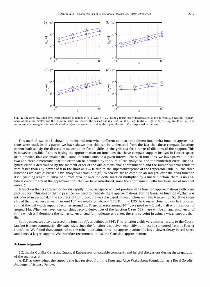
e are all second-order accurate we expect from Eq. (109) to see second-order convergence when theerror is measured away from C. We recall that analytical results suggested that g P x is needed to obtain the convergenceorder of the delta function approximation, see Eq. (109). However, our numerical simulations indicate that g ¼ e is sufficient.In Fig. 12 the maximum norm and the L1-norm of the error is shown for dFD

2h ; dG2h; d

TE2h, and dC

2h. For the regularized delta func-tion dC

2h of order h4 in one dimension there is no convergence, neither in the maximum norm nor in the L1-norm. Note thatthe error using dG

2h is almost identical to the error we obtain using dTE2h.

We obtained similar results for other values of x away from the boundary of the computational domain.

7. Conclusions

We have introduced delta function approximations that are convenient to use for delta functions with support on a curvein 2D or a surface in 3D, represented implicitly by a level set. The framework is based on the ‘‘old” method with a one-dimen-sional delta function approximation extended to higher dimensions by a distance function.

Fig. 10. The exact solution uðxÞ given by Eq. (111) for x ¼ 0.

10−2 10−110−4

10−3

10−2

10−1

100

h

||uh−u

|| ∞

10−2 10−110−4

10−3

10−2

10−1

100

h

||uh−u

|| ∞

The maximum norm of the error measured over X is shown for dmh;m ¼ 1 (circles), m ¼ 2 (stars), and m ¼ 3 (squares). A fourth-order discretizationdifferential operator has been used. The dashed line is y ¼ h. In (a) dmh ¼ dFD

mh is used. In (b) dmh ¼ dGmh is used. As expected, we see a first-order error,

e have measured the error also close to C.

10−2 10−110−6

10−4

10−2

100

h

||uh−u

||

10−2 10−110−6

10−4

10−2

100

h

||uh−u

||10−2 10−110−6

10−4

10−2

100

h

||uh−u

||

10−2 10−110−6

10−4

10−2

100

h||u

h−u||

Fig. 12. The error measured over eX (this domain is defined in (113) with g ¼ 0:2) using a fourth-order discretization of the differential operator. The max-norm of the error (circles) and the L1-norm (stars) are shown. The dashed line is y ¼ h2. In (a) de ¼ dFD

2h . In (b) de ¼ dG2h . In (c) de ¼ dTE

2h . In (d) de ¼ dC2h . The

second-order convergence is now obtained in (a)–(c), as we are excluding the region closest to C, as explained in the text.


This method was in [3] shown to be inconsistent when different compact one-dimensional delta function approxima-tions were used. In this paper, we have shown that this can be understood from the fact that these compact functionscannot both satisfy the discrete mass condition for all shifts in the grid and for a range of dilations of the support. Thisis however possible if one is basing the approximation on functions that have compact support instead in Fourier space,or in practice, that are smaller than some tolerance outside a given interval. For such functions, we have proven in bothtwo and three dimensions that the error can be bounded by the sum of the analytical and the numerical error. The ana-lytical error is determined by the moment order of the one-dimensional approximation and the numerical error tends tozero faster than any power of h in the limit as h! 0, due to the superconvergence of the trapezoidal rule. All the threefunctions we have discussed have analytical errors of Oðh2Þ. When we are to compute an integral over the delta functionitself, yielding length of curve or surface area, or over the delta function multiplied by a linear function, there is no ana-lytical error for any of the approximations that we have introduced, since the approximate delta functions are of momentorder 2.

A function that is compact or decays rapidly in Fourier space will not produce delta function approximations with com-pact support. This means that in practice, we need to truncate these approximations. For the Gaussian function dG

e , that wasintroduced in Section 4.2, the accuracy of this procedure was discussed in conjunction with Fig. 6 in Section 5.3. It was con-cluded that to achieve an error around 10�6 we need e P mh;m ¼ 1:25. For m ¼ 1:25 the Gaussian function can be truncatedso that the half width support becomes around 6h. To get an error around 10�16, we need m ¼ 2 and a half width support ofaround 14h. When we have non-vanishing second derivatives of the function F, see (57), there will be an analytical error ofOðh2Þ which will dominate the numerical error, and for moderate grid sizes, there is no point in using a wider support than6h.

In this paper, we also discussed the function dTEe , as defined in (44). This function yields very similar results to the Gauss-

ian, but is more computationally expensive, since the function is not given explicitly but must be computed from its Fouriertransform. We found that, compared to the other approximations, the approximation dFD

e , has a slower decay in real spaceand hence a larger support. We therefore recommend to use the Gaussian approximation.

Acknowledgment

S.Z. thanks Gunilla Kreiss and Emanuel Rubensson for valuable comments and helpful discussions during the preparationof the manuscript.

A.-K.T. acknowledges the support she has received from the Knut and Alice Wallenberg Foundation as a Royal SwedishAcademy of Science Fellow.


Appendix A. We start by stating a definition and a theorem from Ref. [19] that will be used in the study of the analyticalerror in three dimensions.

Definition 8.1. Let k > 0. A k-manifold in Rn of class Cr is a subspace M of Rn having the following property: For each p 2 M,there is an open set V of M containing p, a set U that is open in either Rk or the upper half-space in Rk and a continuous mapP : U ! V carrying U onto V in one-to-one fashion, such that:

1. P is of class Cr .2. P�1 : V ! U is continuous.3. DPðxÞ, the Jacobian matrix of P, has rank k for each x 2 U.

The map P is called a coordinate patch on M about p.

Theorem 8.1. Let M be a compact k-manifold in Rn, of class Cr. Let f : M ! R be a continuous function. Suppose that Pi : Ai ! Mi,for i ¼ 1; . . . ;N is a coordinate patch on M, such that Ai is open in Rk and M is the disjoint union of the open sets M1; . . . ;MN of Mand a set K of measure zero in M. Then
Z
MfdV ¼

XN

i¼1

ZAi

ðf � PiÞVðDPiÞ: ð114Þ

This theorem states thatR

M fdV can be evaluated by separately evaluating the integral over local parametrized parts of themanifold and then summing up all the contributions. A proof of the theorem can be found in Ref. [19]. It is assumed that thesupport of the integrand f lies in M.

Proof of Theorem 5.2. In three dimensions we cannot expect to have a global parametrization but a local exist. By theassumption C is a 2-manifold that can be covered by an union of disjoint open sets V1; . . . ;Vl and a set K of measure zero in C.It has been proven that such sets can be constructed using polygonal charts sets, see [20]. Further, we have assumed that acoordinate patch Pj ¼ ðxðr; sÞ; yðr; sÞ; zðr; sÞÞ : ðr1; r2Þ � ðs1; s2Þ ! Vj of class C2 on C exists.

The normal of C at Vj is defined as n ¼ ðn1;n2;n3Þ ¼ 1qðr;sÞ ðP

jr � Pj

sÞ, where qðr; sÞ ¼ kPjr � Pj

sk – 0.

The integration is over Xx. This is a compact 3-manifold of class C2. The integrand deF : Xx ! R, is a continuous function.The domain Xx can be covered by the disjoint union of open sets M1; . . . ;Ml and a set of measure zero in Xx. The open set Mj

can be given by the following parametrization

Mj ¼ fðx; y; zÞ : x ¼ Xjðr; s; tÞ; y ¼ Yjðr; s; tÞ; z ¼ Zjðr; s; tÞ; r 2 ðr1; r2Þ; s 2 ðs1; s2Þ; t 2 ½�x;x�g; ð115Þ

where Xjðr; s; tÞ ¼ xðr; sÞ þ tn1ðr; sÞ;Yjðr; s; tÞ ¼ yðr; sÞ þ tn2ðr; sÞ, and Zjðr; s; tÞ ¼ zðr; sÞ þ tn3ðr; sÞ. LetAj ¼ ðr1; r2Þ � ðs1; s2Þ � ½�x;x�, and

bj ¼ ðXjðr; s; tÞ; Yjðr; s; tÞ; Zjðr; s; tÞÞ: ð116Þ

Then it follows from Theorem 8.1 that:

IXx ðdeFÞ ¼Xl

j¼1

IAj¼Xl

j¼1

ZAj

ðde � bjÞðF � bjÞVðDbjÞ; ð117Þ

where VðDbjÞ ¼ jdetðJðr; s; tÞÞjdtdsdr. The Jacobian determinant for this transformation from ðx; y; zÞ to ðr; s; tÞ is

detðJðr; s; tÞÞ ¼ ðXjr; Y

jr ; Z

jrÞ � ðX

js;Y

js; Z

jsÞ ðX

jt ;Y

jt ; Z

jtÞ ¼ ðP

jr � Pj

s þ tðnr � Pjs þ Pj

r � nsÞ þ t2ðnr � nsÞÞ n

¼ kPjr � Pj

skð1� tðj1 þ j2Þ þ t2j1j2Þ ¼ qðr; sÞð1� tj1ðr; sÞÞð1� tj2ðr; sÞÞ: ð118Þ

Here we have used that the coordinate patch, Pj is C2 hence Pjrs ¼ Pj

sr . This transformation is non-singular because of theassumption in Eq. (68)

Note that dðC;xÞ ¼ t and denote

f ðr; s; tÞ ¼ FðXjðr; s; tÞ; Yjðr; s; tÞ; Zjðr; s; tÞÞ: ð119Þ

We have

IAj¼Z

Aj

ðde � bjÞðF � bjÞVðDbjÞ ¼Z r2

r1

Z s2

s1

Z x

�xdeðtÞf ðr; s; tÞqðr; sÞð1� tj1ðr; sÞÞð1� tj2ðr; sÞÞdtdsdr: ð120Þ

The assumption that FðxÞ is a smooth function yields that f ðr; s; tÞ has N þ 1 bounded derivatives with respect to t. Sincet 2 ½�x;x� we can for x small Taylor expand f ðr; s; tÞ around ðr; s;0Þ


f ðr; s; tÞ ¼XN

i¼0

ti

i!fitðr; s;0Þ þ OðtNþ1Þ: ð121Þ

The index i in fit denotes the number of partial derivatives with respect to t. Define the moments of the function deðtÞ as

MaðdeðtÞÞ ¼Z x

�xdeðtÞtadt: ð122Þ

Replacing f ðr; s; tÞ in Eq. (120) with its Taylor expansion we obtain

IAj¼ M0ðdeðtÞÞ

Z r2

r1

Z s2

s1

f ðr; s; 0Þqðr; sÞdsdr

þM1ðdeðtÞÞZ r2

r1

Z s2

s1

ftðr; s;0Þqðr; sÞdsdr �Z r2

r1

Z s2

s1

f ðr; s; 0Þqðr; sÞðj1ðr; sÞ þ j2ðr; sÞÞdsdr

þXN

a¼2

Cja;FMaðdeðtÞÞ þ OðMNþ1ðdeðtÞÞÞ; ð123Þ

where the constant Cja;F is given in Eq. (71).

By the change of variable t=e ¼ n and since x ¼ pe we get

MaðdeðtÞÞ ¼Z x

�x

1euðt=eÞtadt ¼ ea

Z p

�puðnÞnadt: ð124Þ

By summing up contributions from all Aj we obtain the theorem. h

References

[1] S. Osher, J.A. Sethian, Fronts propagating with curvature dependent speed: Algorithms based on Hamilton–Jacobi formulations, J. Comput. Phys. 79(1988) 12–49.

[2] S. Osher, R. Fedkiw, Level Set Methods and Dynamic Implicit Surfaces, Springer Verlag, 2003.[3] A.-K. Tornberg, B. Engquist, Numerical approximations of singular source terms in differential equations, J. Comput. Phys. 200 (2004) 462–488.[4] C.S. Peskin, The immersed boundary method, Acta Numer. 11 (2002) 479–517.[5] J. Sethian, Level Set Methods and Fast Marching Methods, Cambridge University Press, 1999.[6] B. Engquist, A.-K. Tornberg, R. Tsai, Discretization of dirac delta functions in level set methods, J. Comput. Phys. 207 (2005) 28–51.[7] P. Smereka, The numerical approximation of a delta function with application to level set methods, J. Comput. Phys. 211 (2006) 77–90.[8] J.T. Beale, A proof that a discrete delta function is second-order accurate, J. Comput. Phys. 227 (2008) 2195–2197.[9] J.D. Towers, Two methods for discretizing a delta function supported on a level set, J. Comput. Phys. 220 (2007) 915–931.

[10] J.D. Towers, A convergence rate theorem for finite difference approximations to delta functions, J. Comput. Phys. 227 (2008) 6591–6597.[11] A.-K. Tornberg, B. Engquist, Regularization techniques for numerical approximation of pdes with singularities, J. Scient. Comp. 19 (2003) 527–552.[12] A.-K. Tornberg, Multi-dimensional quadrature of singular and discontinuous functions, BIT 42 (2002) 644–669.[13] E. Olsson, G. Kreiss, A conservative level set method for two phase flow, J. Comput. Phys. 210 (2005) 225–246.[14] E. Olsson, G. Kreiss, S. Zahedi, A conservative level set method for two phase flow II, J. Comput. Phys. 225 (2007) 785–807.[15] R.P. Beyer, R.J. Leveque, Analysis of a one-dimensional model for the immersed boundary method, SIAM J. Numer. Anal. 29 (2) (1992) 332–364.[16] B.E. Segee, Using spectral techniques for improved performance in artificial neural networks, pp. 500–505.[17] G. Dahlquist, Å. Björck, Numerical Methods in Scientific Computing, SIAM, 2008.[18] P.J. Davis, P. Rabinowitz, Numerical Integration, Blaisdel Publishing Company, 1967.[19] J.R. Munkres, Analysis on Manifolds, Westview Press, 1991.[20] J.R. Munkres, Elementary differential topology, Princeton University Press, 1963.

Delta function approximations in level set methods by distance ...

Documents

Transcript of Delta function approximations in level set methods by distance ...