Abstract Delta Modeling

Dave ClarkeMichiel Helvensteijn

Ina Schaefer

Report CW592, August 2010

Katholieke Universiteit LeuvenDepartment of Computer Science

Celestijnenlaan 200A – B-3001 Heverlee (Belgium)

Abstract Delta Modeling

Dave ClarkeMichiel Helvensteijn

Ina Schaefer

Report CW592, August 2010

Department of Computer Science, K.U.Leuven

Abstract

Delta modeling is an approach to facilitate automated productderivation for software product lines. It is based on a set of deltasspecifying modifications that are incrementally applied to a coreproduct. The applicability of deltas depends on feature-dependentconditions. This paper presents abstract delta modeling, which ex-plores delta modeling from an abstract, algebraic perspective. Com-pared to previous work, we take a more flexible approach with re-spect to conflicts between modifications and introduce the notion ofconflict-resolving deltas. We present conditions on the structure ofdeltas to ensure unambiguous product generation.

Keywords : Software Product Lines; Automated Product Derivation; DeltaModeling; Conflict Resolution.

Abstract Delta Modeling ∗

Dave ClarkeIBBT-DistriNet, Katholieke Universiteit

Leuven, Belgiumdave.clarke@cs.kuleuven.be

Michiel HelvensteijnCWI, Amsterdam LIACS, Leiden

University, The Netherlandsmichiel.helvensteijn@cwi.nl

Ina Schaefer †

Chalmers University of Technology,Gothenburg, Swedenschaefer@chalmers.se

AbstractDelta modeling is an approach to facilitate automated productderivation for software product lines. It is based on a set of deltasspecifying modifications that are incrementally applied to a coreproduct. The applicability of deltas depends on feature-dependentconditions. This paper presents abstract delta modeling, whichexplores delta modeling from an abstract, algebraic perspective.Compared to previous work, we take a more flexible approach withrespect to conflicts between modifications and introduce the notionof conflict-resolving deltas. We present conditions on the structureof deltas to ensure unambiguous product generation.

This report is an extended version of a paper to appear inGPCE’10.

Keywords Software Product Lines; Automated Product Deriva-tion; Delta Modeling; Conflict Resolution.

1. IntroductionA software product line (SPL) is a set of software systems, calledproducts, with well-defined commonalities and variabilities [11,34]. Software product line engineering aims at developing this setof systems by reuse in order to reduce time to market and to in-crease product quality. Automated product derivation (or softwaremass customization [24]) is an approach to generating individualproducts without the need for manual intervention during applica-tion engineering, which can be tedious and error-prone [13].

Currently, product line variability is mostly represented byfeature models [19, 42]. Features are designated product charac-teristics or increments of product functionality [7]. A product isuniquely identified by a valid feature configuration, i.e., a legalcombination of features from the feature model. On the featuremodel level, features are merely labels [12]. In order to be able toautomatically derive a product for a particular feature configura-tion, a correspondence between the features on the feature mod-eling level and the reusable product line artifacts has to be intro-duced. Additionally, the product line artifacts have to be organized

∗ This research is partly funded by the EU project FP7-231620 HATS:Highly Adaptable and Trustworthy Software using Formal Methods(http://www.hats-project.eu)† This author is supported by the German Science Foundation (DFG).

[Copyright notice will appear here once ’preprint’ option is removed.]

in such a way that they can be assembled automatically to generatea uniquely determined product.

Feature-oriented programming [7] is a prominent approach forimplementing SPLs by composition of feature modules that di-rectly correspond to product features. Delta modeling [37–39]extends feature-oriented programming. In the delta modeling ap-proach, a product line is represented by a core product and a setof product deltas. Product deltas specify modifications to the coreproduct to generate further products of the product line. Each deltahas an application condition specifying for which feature configu-rations the modifications have to be carried out, connecting featureson the feature modeling level with product line artifacts. A productfor a feature configuration can be obtained by applying those prod-uct deltas with a valid application condition to the core product.

In this paper, we generalize the existing delta modeling ap-proaches [37–39] and present an abstract, algebraic formalizationof the delta modeling concepts. The presented abstract delta mod-eling approach goes beyond existing work with its novel treatmentof conflicts between deltas. A conflict between deltas arises if theirspecified modifications do not commute. This means that applyingthem in different orders results in different (composed) modifica-tions. In previous work, deltas were either incomparable [37, 39],which required writing additional deltas for every conflicting com-bination, or they had to be ordered in a very restrictive way [38]to avoid conflicts explicitly. As a main contribution of this paper,we introduce the notion of conflict-resolving deltas that relax theserestrictions and make delta modeling of product lines more flexi-ble. A conflict-resolving delta, which is applied after two conflict-ing deltas, eliminates differences between the (composed) modi-fications. If for every pair of conflicting deltas a conflict-resolvingdelta exists, all possible sequences of deltas produce the same mod-ification and generate a uniquely defined product. In order to ensurethis result for every valid feature configuration, we provide efficientconditions requiring only the inspection of the product line directly,without having to generate and check all products.

The concepts of abstract delta modeling can be instantiated fordifferent kinds of development artifacts, such as documentation,models or code. We demonstrate the feasibility of the approach bypresenting an instantiation of abstract delta modeling for object-oriented implementations of software product lines and extendthis with method wrapping. Furthermore, we show that existingformalizations of compositional product line implementations canbe seen as instantiations of abstract delta modeling.

The abstract delta modeling formalism consists of a number ofingredients, which are depicted in Figure 1, along with the opera-tions between them. At the top is (a model of) the software productline that is defined by the feature model, the core product, the prod-uct deltas specifying modifications of the core product, a partialordering on the deltas restricting their application and the applica-tion conditions for the deltas. By specifying a feature configuration,one can produce a delta model, consisting of an ordered collection

1 2010/8/9

Product Line: PL = (Φ, c,D,≺, γ) (Def. 15)

Delta Model: (D,≺) (Def. 2)

Composite Delta: x = xn · . . . ·x1 (Def. 1)

Product→ Product: f Product (Def. 16)

feature configuration: PL�F (Def. 16)

derivation: derv(D,≺) (Def. 3)

partial delta application:x(−) (Defs. 10,11)

delta application to core:x(c) (Defs. 10,11)

application tocore: f(c)

Figure 1. Relationship between artefacts. Relevant definitionnumbers are indicated in parentheses.

of modifications necessary to generate the respective product. Theprocess of derivation applied to a delta model puts the specifiedmodifications in a linear order that is compatible with the partialordering in order to obtain a valid, ideally unique, composed mod-ification. The partial delta application operation applied to a deltareturns a function that takes a product and produces a new product.This function can then be applied to the core product to produce thetarget product for a given feature configuration.

This paper is organized as follows. Section 2 presents deltamodels and criteria for their unambiguity. Sections 3 and 4 rein-troduce products and incorporate deltas into product lines, trans-ferring the unambiguity properties. Section 5 presents a concreteclass of deltas and illustrates our approach using an example. Sec-tion 6 compares our approach with existing algebraic approachesfrom the literature. Finally, Sections 7 and 8 present related workand conclusions.

2. Abstract Delta ModelingThis section presents our approach of abstract delta modeling. Weintroduce product modifications and their composition as a monoid,called a deltoid. Delta models are built on top of this monoid aspartially ordered collections of modifications, where the orderingconstrains the possible ways such modifications can be applied. Itis important that a delta model defines unambiguous modificationsas these are used later to obtain distinct products. Thus, we definethe notions of conflict, leading to ambiguous modifications, andconflict-resolving deltas eliminating these. We develop conditionsto ensure that a delta model is unambiguous.

2.1 Delta ModelsIn existing compositional approaches for implementing softwareproduct lines, such as feature-oriented programming [7] or delta-oriented programming [38], a member product of an SPL is ob-tained by the application of a number of modifications (deltas)x1, . . . , xn to a core product c, as follows:

xn(· · ·x1(c) · · ·).In feature-oriented programming the core product is determined byone or more base modules. The modifications are feature modulesextending and refining the core product. In delta-oriented program-ming the core product can be any valid product of the product line.

As both approaches treat the core product as a constant elementfor all products in the product line, it is useful to focus on themodifications. In this setting, the above modification would be

equivalently written as follows, where · refers to the compositionof modifications:

(xn · . . . ·x1)(c).

Thus, we will focus exclusively on sequences of modifications suchas xn · . . . ·x1.

It may still be possible to reason about the core product if wechoose to see it as a modification xc applied to the empty product0, i.e. c = xc(0). Thus:

(xn · . . . ·x1)(c) = (xn · . . . ·x1 ·xc)(0),

so nothing is lost by restricting our attention to modifications.In abstract delta modeling the main object of interest is a del-

toid. A deltoid consists of a set of modifications, called deltas,along with the operation for composing them sequentially. A del-toid can contain different kinds of deltas for different kinds of de-velopment artefacts (e.g., documentation, models or code) and fordifferent levels of abstraction (e.g., when working on componentlevel or working on class level). The concrete nature of the modifi-cations specified in the deltas depends on the capabilities of the un-derlying modeling or programming languages. Deltas may be func-tions performing the changes directly or some other structure rep-resenting those changes. We abstract away from the internal detailsof modifications, since many different instantiations are possible.

We define the notions of deltoids and deltas as follows.

Definition 1 (Deltoid). A deltoid is a monoid (D, ·, ε), where Dis a set of modifications (referred to as deltas), and the operation· : D ×D → D corresponds to their sequential composition. y ·xdenotes the modification applying first x and then y. The neutralelement ε of the monoid corresponds to modifying nothing.

The operation · is associative but not inherently commutative,as the ordering between two deltas may be significant. We call twodeltas x, y ∈ D incompatible if y ·x 6= x · y.

A delta model describes the collection of deltas required to builda specific product, along with a strict partial ordering on thosedeltas restricting the order in which they can be applied. Recallthat a strict partial order is irreflexive, asymmetric and transitive.

Definition 2 (Delta Model). A delta model is a tuple (D,≺), whereD ⊆ D is a finite set of deltas and ≺ ⊆ D ×D is a strict partialorder on D. x ≺ y states that x should be applied before, thoughnot necessarily directly before, y.

The partial order between deltas represents the intuition that asubsequent delta has full knowledge of (and access to) earlier deltasand more authority over modifications to the product. This is real-ized by applying the deltas in a linear extension of the partial order,as shown in the following definition. A derivation is a sequentialcomposition of all deltas in a model to generate a desired product.

Definition 3 (Derivation). Given a delta model P = (D,≺), itsderivations are defined to be

derv(P )def=

xn · . . . ·x1 | x1, . . . , xn is a linear extension

of ≺ where {x1, . . . , xn} = D

ff.

Note that derv(P ) may potentially generate more than one dis-tinct derivation as incompatible deltas may be applied in differentorderings. However, it is desirable that all possible derivations of adelta model have the same effect, as this corresponds to deriving aunique product. This motivates the following definition.

Definition 4 (Unique Derivation). A delta model P = (D,≺) issaid to have a unique derivation iff xn · . . . ·x1 = x′n · . . . ·x′1 forall pairs of linear extensions (x1, . . . , xn) and (x′1, . . . , x

′n) of ≺.

Or, equivalently, iff | derv(P )| = 1.

2 2010/8/9

2.2 Unambiguity of Delta ModelsThe property that a delta model has a unique derivation can bechecked by brute force. This means generating all possible deriva-tions (in the worst case, n! for n deltas), and then checking that theyall correspond. In order to allow for a more efficient way to estab-lish this property, we introduce unambiguous delta models whichrely on the notion of conflicting deltas and conflict resolving deltas.

Two deltas are in conflict if they are incompatible and no order-ing is placed upon them. Intuitively, the two conflicting deltas areindependently modifying the same part of the product in differentways, meaning that multiple distinct derivations may be possible.

Definition 5 (Conflict). Given a delta model P = (D,≺),x, y ∈ D are said to be in conflict iff the following condition holds:

x E y def= y ·x 6= x · y ∧ x 6≺ y ∧ y 6≺ x.

One way to ensure a unique derivation is to avoid conflicts byalways enforcing an ordering between incompatible deltas [38].However, features with conflicting implementations are often in-dependent in concept. Kastner et al. [23] call the issue of how tomodel such situations the optional feature problem. Imposing anordering on the deltas of conceptually orthogonal features is of-ten inappropriate. Some (unrelated) functionality may be inadver-tently and silently overwritten. Furthermore, sometimes neither ofthe original choices in functionality is exactly what we need, andsome combination of them should be used.

The alternative is to allow conflicts but to provide additional,subsequently applied, deltas to resolve them.

Notation 1. IfD ⊆ D, thenD∗ andD+ denote the sequences andnon-empty sequences of compositions of deltas from D.

Definition 6 (Conflict-Resolving Delta). Given a delta model P =(D,≺) and x, y ∈ D which are in conflict, we say that a deltaz ∈ D resolves their conflict iff the following property holds:

(x, y) C zdef=

x ≺ z ∧ y ≺ z ∧∀d ∈ D∗ : z · d · y ·x = z · d ·x · y.

An unambiguous delta model is now a delta model contain-ing a conflict-resolving delta for every conflicting pair of deltas.Conflict-resolving deltas take the role of derivative modules [23]or lifters [35]. They contain only the functionality necessary whenseveral interacting features are selected together.

Definition 7 (Unambiguous Delta Model). Given a delta model(D,≺), we say that the model is unambiguous iff

∀x, y ∈ D : x E y ⇒ ∃z ∈ D : (x, y) C z.

If a delta model is unambiguous, we can show that it has aunique derivation. In order to prove this, we need some interme-diate results. Lemma 1 states that in an unambiguous delta model,any two deltas in a derivation are either ordered or commutative.

Lemma 1. Given an unambiguous delta model P = (D,≺) andd2 · y ·x · d1 ∈ derv(P ), where x, y ∈ D and d1, d2 ∈ D∗. Theneither x ≺ y or d2 · y ·x · d1 = d2 ·x · y · d1.

Proof. By case distinction on the unambiguity of P for deltasx and y:

• Case y ·x = x · y. It follows that d2 · y ·x · d1 = d2 ·x · y · d1.• Case x ≺ y. Immediate.• Case y ≺ x. Cannot happen, otherwise d2 · y ·x · d1 would not

be a linear extension of ≺.• Case ∃z ∈ D : (x, y) C z. Firstly, from the definition of con-

flict resolving delta we have that x, y ≺ z, hence there existd′2, d

′′2 ∈ D∗ such that d2 · y ·x · d1 = d′2 · z · d′′2 · y ·x · d1.

From the remaining condition on z, we have z · d′′2 · y ·x =

z · d′′2 ·x · y, hence d2 · y ·x · d1 = d′2 · z · d′′2 · y ·x · d1 =d′2 · z · d′′2 ·x · y · d1 = d2 ·x · y · d1.

Lemma 2 states that removing a minimal element with respectto the partial order preserves unambiguity of delta models.

Lemma 2. If P = (D,≺) is an unambiguous delta model and wis minimal in ≺, then (D \ {w} ,≺′), where ≺′ is ≺ restricted toD \ {w}, is also an unambiguous delta model.

Proof. If (D,≺) is unambiguous, then ∀x, y ∈ D : x E y ⇒ ∃z ∈D : (x, y) C z. For this to be true inD\{w} we need to show thatthere are no x and y such that x E y with w such that (x, y) C w.But w could not have been a conflict resolver, as it is minimal,contradicting conditions x ≺ w and y ≺ w of (x, y) C w.

Lemma 3 formulates that a minimal element in the partial ordercan be moved to the front of any derivation from an unambiguousdelta model without changing the meaning of that derivation.

Lemma 3. Given an unambiguous delta model P = (D,≺). Letxn · . . . ·x1 ∈ derv(P ), where {x1, . . . , xn} = D, with xi mini-mal in ≺. Then xn · . . . ·x1 = xn · . . . ·xi+1 ·xi−1 · . . . ·x1 ·xi.

Proof. By induction on i:

• Case i = 1. Immediate.• Case i > 1. Since xi−1 6≺ xi, as xi is minimal, Lemma 1 im-

plies that xn · . . . ·x1 = xn · . . . ·xi+1 ·xi−1 ·xi ·xi−2 · . . . ·x1.By induction, xn · . . . ·xi+1 ·xi−1 ·xi ·xi−2 · . . . ·x1 =xn · . . . ·xi+1 ·xi−1 · . . . ·x1 ·xi.

The following theorem states that every unambiguous deltamodel has a unique derivation. This reduces the effort of checkingthat all possible derivations of a delta model have the same effectto checking that all conflicts between pairs of deltas are eliminatedby conflict resolving deltas. The proof is by induction over the sizeof the delta model.

Theorem 1. An unambiguous delta model has a unique derivation.

Proof. Given unambiguous delta model P = (D,≺). Proceed byinduction on the size of D:

• Case |D| = 0. Immediate as derv(P ) = {ε}.• Case |D| = 1. Immediate as derv(P ) = {x}, whereD = {x}.• Case |D| > 1. For any two d1, d2 ∈ derv(P ), let d1 = d′1 ·x

and d2 = d′2 ·x · d′′2 , where x ∈ D and d′1, d′2, d′′2 ∈ D∗. Asx is the last element of d1, it must be minimal in ≺. Thus,by Lemma 3, d′2 ·x · d′′2 = d′2 · d′′2 ·x. Now by Lemma 2,P ′ = (D \ {x} ,≺′), where ≺′ is ≺ restricted to D \ {x}, isan unambiguous delta model, and d′1, d′2 · d′′2 ∈ derv(P ′). Bythe induction hypothesis, d′1 = d′2 · d′′2 and thus d1 = d′1 ·x =d′2 · d′′2 ·x = d2. Hence, | derv(P )| = 1.

2.3 Consistent Conflict ResolutionAlthough the notion of unambiguous delta model alleviates thetask of establishing that a delta model has a unique derivation,unambiguity is still quite complex to check. The reason is that thedefinition of a conflict resolving delta (Definition 6) quantifies overall elements ofD∗. Hence, in order to check that a delta is indeed aconflict resolver, all these sequences of deltas have to be inspected.However, for interesting classes of deltoids, a simpler criterionexists to make checking ambiguity more feasible. The consistentconflict resolution property states that if a delta z resolves an (x, y)-conflict when it is applied directly after x and y, it also resolves theconflict after the application of any sequence of intermediate deltas.

3 2010/8/9

Definition 8 (Consistent Conflict Resolution). A deltoid (D, ·, ε)is said to exhibit consistent conflict resolution iff the followingcondition holds:∀x, y, z ∈ D :

z · y ·x = z ·x · y ⇒ ∀d ∈ D : z · d · y ·x = z · d ·x · y.If a deltoid (D, ·, ε) exhibits consistent conflict resolution, then adelta model (D,≺) withD ⊆ D is also said to exhibit the property.

Note that the consistent conflict resolution property is checkedat the level of the underlying deltoid, rather than for any specificdelta model. Hence, it has to be established only once for a givendeltoid and then holds for all delta models based on that deltoid.

To establish the unambiguity of a delta model exhibiting con-sistent conflict resolution, it is sufficient to check that for each pairof conflicting deltas x and y there exists a conflict-resolving deltaz, such that x ≺ z ∧ y ≺ z ∧ z · y ·x = z ·x · y. We need notquantify over all possible intermediate sequences of deltas. Con-sequently, unambiguity of delta models can be established muchmore efficiently. This is formalized in the next theorem.

Theorem 2. Given delta model P = (D,≺) exhibiting consis-tent conflict resolution, for all deltas x, y, z ∈ D, it is true thatx ≺ z ∧ y ≺ z ∧ z · y ·x = z ·x · y =⇒ (x, y) C z.

Proof. From the definition of consistent conflict resolution, wehave the following:

z · y ·x = z ·x · y ⇒ ∀d ∈ D : z · d · y ·x = z · d ·x · y⇒ ∀d ∈ D∗ : z · d · y ·x = z · d ·x · y,

which may be substituted into x ≺ z ∧ y ≺ z ∧ z · y ·x = z ·x · yto form the definition of (x, y) C z.

3. Reintroducing ProductsThus far, only modifications have been considered, without consid-ering the products that we modify. Products can be reintroduced,by defining the notion of application of a delta to a product. Firstly,we select a set of products.

Definition 9 (Products). Let P denote a set of possible products.

Applying a delta to a product results in another product. This iscaptured by the notion of delta application.

Definition 10 (Delta Application). Delta application is an opera-tion −(−) : D × P → P . If d ∈ D and p ∈ P , then d(p) ∈ P isthe product resulting from applying delta d to product p.

This definition implies that one generates a product from asequence of deltas by first composing the deltas and then applyingthe result to the core product. A much stronger version of deltaapplication is possible, borrowing the notion of monoid action.

Definition 11 (Delta Action). A delta application operation−(−) :D × P → P is called a delta action if it satisfies the conditions(y ·x)(p) = y(x(p)) and ε(p) = p, for all x, y ∈ D and p ∈ P .

This generalises the case when · is function composition and−(−) is function application.

4. Product LinesUsing the introduced concepts of delta models, products and deltaapplication we can now abstractly define product lines, thus provid-ing a link from feature configurations on the feature modeling levelto product representations. We will extend the concept of unambi-guity to the level of product lines and provide an efficient conditionto check unambiguity.

4.1 Defining Product LinesProduct line variability is predominantly captured by featureswhere a feature captures a designated product characteristic or anincrement to product functionality. At the level of the feature modelfeatures are merely labels without inherent semantic meaning. Aproduct can be characterized by the set of features it provides.

Definition 12 (Features). Let F denote a universal set of features.

The set of products in a product line can be represented by afeature model. Many formal descriptions [17, 19, 42] agree that afeature model determines a set of valid feature configurations.

Definition 13 (Feature Model). A feature model Φ ⊆ P(F) isa set of sets of features from F . Each F ∈ Φ is a set of featurescorresponding to a valid feature configuration.

In order to bridge the gap between features and product lineartifacts, we introduce application conditions for deltas. An appli-cation condition attached to a delta determines for which featureconfiguration the delta has to be applied.

Definition 14 (Application Function and Condition). Let D ⊆ Dbe a set of deltas. An application function γ : D → P(P(F))gives the feature configurations each delta x ∈ D is applicableto. Thus, F ∈ γ(x) denotes that delta x is applicable for featureconfiguration F . γ(x) is called the application condition for x.

A product line is defined by its feature model, characterizing allmember products by a set of valid feature configurations, the coreproduct, the associated delta model, containing the modificationsused to obtain further products, and the application function, asso-ciating features and deltas. None of these elements can be inferredfrom the other elements.

Definition 15 (Product Line). A product line is a tuple (Φ, c,D,≺, γ),where Φ is a feature model, c ∈ P is the core product, (D,≺) is adelta model and γ is an application function with domain D.

If feature configuration F is valid according to Φ, its corre-sponding product is defined by the delta model containing only thedeltas applicable to F . Selecting such deltas gives a delta modelwhose derivations applied to the core product correspond to the de-sired product for feature configuration F .

Definition 16 (Selected Delta Model). Given a product line PL =(Φ, c,D,≺, γ), a selected delta model for feature configurationF ∈ Φ, denoted PL � F , is the delta model (D′,≺′) whereD′ = { d ∈ D | F ∈ γ(d) } is the set of applicable deltas, and≺′ is ≺ restricted to D′.

We now define the set of products generated from a product line.

Definition 17 (Generated Products). Given a product line PL =(Φ, c,D,≺, γ), the set of generated products for feature configu-ration F ∈ Φ is defined as follows:

prod(PL, F )def= {x(c) | x ∈ derv(PL�F ) } .

4.2 Unambiguity of Product LinesAs argued in Section 2, unambiguity of delta models is a desiredproperty because it ensures unique derivation and, consequently, aunique generated product. We now lift unambiguity to the productline level. A product line is unambiguous if every selected deltamodel is unambiguous. This means that every valid feature config-uration yields a uniquely defined product, which is an importantcondition for the applicability of automated product derivation.

Definition 18 (Unambiguous Product Line). A product line PL =(Φ, c,D,≺, γ) is unambiguous iff

∀F ∈ Φ : PL�F is an unambiguous delta model.

4 2010/8/9

The unambiguity of a product line can be checked by generat-ing the selected delta models of all valid feature configurations andchecking unambiguity by the criteria proposed in Section 2. How-ever, as the set of feature configurations is often exponential in thenumber of features, that naive approach would be rather expensive.Instead, we propose the notion of a globally unambiguous productline that implies product line unambiguity.

We first introduce a shorthand notation for the set of featureconfigurations for which two deltas x and y are applicable.

Notation 2. Given a product-line (Φ, c,D,≺, γ), the set of validfeature configurations to which the deltas x, y ∈ D apply isdenoted:

Vx,y def= Φ ∩ γ(x) ∩ γ(y).

A product line is globally unambiguous if for any two conflict-ing deltas x and y applied together for a set of feature configu-rations, there is a conflict-resolving delta z applicable in at leastthe same set of feature configurations. Thus for any selected deltamodel in which x and y appear together, the conflict is resolvedby the same delta z. Global unambiguity of a product line can bechecked by inspecting the product line only once and does not re-quire all selected delta models to be generated.

Definition 19 (Globally Unambiguous Product Line). A productline (Φ, c,D,≺, γ) is called globally unambiguous if and only if

∀x, y ∈ D : Vx,y = ∅∨ x E y ⇒ ∃z ∈ D : (Vx,y ⊆ γ(z) ∧ (x, y) C z).

The following theorem states that any globally unambiguousproduct line is also an unambiguous product line. Hence, it sufficesto check global unambiguity by inspecting the product line once toensure that all products that can be generated from the product lineare uniquely determined. In the following proof, we annotate theE and C operators with the delta model for which they apply, e.g.,x EP y and (x, y) CP z.

Theorem 3. A globally unambiguous product line is unambiguous.

Proof. Assume PL = (Φ, c,D,≺, γ) is a globally unambiguousproduct line. Let F ∈ Φ be a valid feature configuration. We showthat P = PL�F = (D′,≺′) is an unambiguous delta model.

Given arbitrary x, y ∈ D′ (so also x, y ∈ D), we perform a caseanalysis on the global unambiguity of PL (Definition 19). Observethat F ∈ γ(x)∩γ(y), otherwise x and y would not be inD′. HenceF ∈ Vx,y . Now for the cases:

• Case Vx,y = ∅. Cannot happen, otherwise x, y /∈ D′.• Case ¬(x E(D,≺) y). So also ¬(x EP y).• Case ∃z ∈ D : Vx,y ⊆ γ(z) ∧ (x, y) C(D,≺) z. Note

that z ∈ D′, as Vx,y ⊆ γ(z). It follows that (x, y) CP z(Definition 16).

So, for all x, y ∈ D′, either ¬(x EP y) or ∃z ∈ D′ : (x, y) CP z.Hence, P is an unambiguous delta model (Definition 7).

A product line can be unambiguous, but not globally unambigu-ous if conflicts between two deltas x and y are resolved by differ-ent conflict-resolving deltas z for different feature configurations.For example, take a product line PL in which the only conflictingdeltas x and y are applied together for feature configurations Fand F ′. For feature configuration F only delta z resolves the con-flict, (x, y) CPL�F z, and for feature configuration F ′ only deltaz′ resolves the conflict, (x, y) CPL�F ′ z′, but z 6= z′. Hence, theproduct line is unambiguous, because the conflict is resolved in allselected delta models, but not globally unambiguous, because theconflict resolving delta is not the same in each one.

5. A Deltoid for Object-Oriented ProgramsWe now present a concrete deltoid for object-oriented programs todemonstrate our approach. In this section, deltas manipulate object-oriented programs on a coarse-grained level. That is, a delta canadd, remove or modify classes. Modifications of classes includeaddition, removal and replacement of fields and methods.

Notation 3. Let f : X⇀Y denote that f is a partial functionfrom X to Y . If f(x) is undefined for x ∈ X , we write f(x) = ⊥,where ⊥ /∈ Y .

Notation 4. Given a set X where − /∈ X , define the notation:

X−def= X ∪ {−} .

5.1 Software ProductsFor simplicity, we abstract from a concrete programming languageas well as from the concrete implementation of methods, and focusonly on the structural aspects of object-oriented programs. First, weintroduce the notion of identifiers for classes, methods and fields.

Definition 20 (Identifiers). Define a global set of identifiers I,used for classes, methods and fields.

Further, we fix an abstract set of method and field definitions.

Definition 21 (Method and Field Definitions). Define a global setof method and field definitionsM.

A class is defined as a partial mapping from identifiers tomethod and field definitions.

Definition 22 (Class Definitions). The collection of class defini-tions is the set of partial functions Ψ = I⇀M. Such a class def-inition ψ ∈ Ψ maps some identifiers to their definition. Unmappedidentifiers are not defined in the class.

As an example, consider the following class definition. Only theexplicitly mentioned identifiers are considered to be defined. Aswe abstract from concrete method implementations, we use capitalletters to refer to method implementations, where different lettersrepresent distinct implementations.

8<:

f 7→ f(): void { A },g 7→ g(): bool { B },i 7→ i: int

9=; .

A program is a set of classes, mapping identifiers to class defi-nitions.

Definition 23 (Programs). Equate the set of products P with theset of programs in an object-oriented language: P = I⇀Ψ.

As an example, consider the following program definition:8>>>><>>>>:

C 7→

8<:

f 7→ f(): void { A },g 7→ g(): bool { B },i 7→ i: int

9=; ,

D 7→

h 7→ h(x: int): int { C },b 7→ b: bool

ff

9>>>>=>>>>;.

5.2 Software DeltasSoftware deltas modify a program by adding, modifying and re-moving classes. A class modification includes adding, replacingand removing methods and fields, or replacing the class completely.

To ensure that composition of deltas produces a closed form,we distinguish between updating a class and replacing it. A classreplacement completely replaces an existing class. A class updatemodifies the original class at the method/field level. Modifying aclass that does not exist is treated as adding a new class. The defini-tion of a software delta captures this set of program modifications.

5 2010/8/9

Definition 24 (Software Deltas). The set of software deltas isdefined asD = I⇀({r}×(I⇀M) ∪ {u}×(I⇀M−))−. Eachdelta d ∈ D is a partial function representing class modifications.r and u represent ‘replace’ and ‘update’, respectively. Mapping anidentifier to − indicates removal from the product. ε = ∅ is theempty delta, modifying nothing.

An example software delta is:8>><>>:

C 7→ u

8<:

f 7→ −,z 7→ z(): void { D },i 7→ i: float

9=; ,

D 7→ −

9>>=>>;.

In contrast to previous work [38], the removal of an elementin this concrete deltoid does not require that the element is alreadypresent, nor does addition require its absence. These simplificationsensure that every derivation of deltas is well-defined.

Now we introduce some notation required in the next few def-initions. The first notation is used to combine two partial func-tions into another partial function by some binary operation on theircodomain.

Notation 5. Use the following notation to lift an operator # ontwo partial functions to the values in their codomain. For i ∈ I:

(a# b)(i)def= a(i) # b(i).

The following notation excludes method and field removalsfrom a class update. Since class replacements should not containremovals, this notation is needed when a class update is sequen-tially composed with a class replacement.

Notation 6. Given class update f : I⇀M−, define f∗ as f , butwithout any method or field removals:

f∗(i)def=

⊥ if f(i) = −f(i) otherwise

Now define sequential composition of software deltas.

Definition 25 (Sequential Composition of Software Deltas). Thesequential composition of software deltas · : D×D → D is definedas

y ·x def= y⊕C x,

where the operator⊕C , working on the level of class modifications,with e, f : I⇀M− and g, h : I⇀M, is

⊕C ⊥ − u f r h⊥ ⊥ − u f r h− − − − −u e u e r e∗ u (e⊕M f) r (e⊕M h)∗

r g r g r g r g r g

and ⊕M , working on the level of method and field definitions, withm,n ∈M, is

⊕M ⊥ − n⊥ ⊥ − n− − − −m m m m .

The options for combining methods are limited, but Section 5.4will redefine ⊕M to allow method wrapping. The definition ofsoftware delta composition gives concrete meaning to the notion ofincompatibility. Two deltas are incompatible if they map the sameidentifier to two different definitions.

Lemma 4. Software deltas are a deltoid.

Proof. We show that · is associative and ∅ is its neutral element.First, we note that if an operator # is associative, then operator

# is associative as well.

For arbitrary a, b, c ∈ M ∪ {−,⊥}, we show that ⊕M isassociative, i.e. (a⊕M b)⊕M c = a⊕M (b⊕M c) by case distinctionon a:

• Case a = ⊥.

(a⊕M b)⊕M c = (⊥⊕M b)⊕M c =b⊕M c = ⊥⊕M (b⊕M c) = a⊕M (b⊕M c).

• Case a = −.

(a⊕M b)⊕M c = (−⊕M b)⊕M c = −⊕M c =− = −⊕M (b⊕M c) = a⊕M (b⊕M c).

• Case a = m for some m ∈M.

(a⊕M b)⊕M c = (m⊕M b)⊕M c = m⊕M c =m = m⊕M (b⊕M c) = a⊕M (b⊕M c).

Thus ⊕M is associative, and then so is ⊕M .For arbitrary a, b, c ∈ {r} × (I⇀M) ∪ {u} × (I⇀M−) ∪

{−,⊥}, we show that ⊕C is associative, i.e. (a ⊕C b) ⊕C c =a⊕C (b⊕C c) by case distinction on a:

• Case a = ⊥.

(a⊕C b)⊕C c = (⊥⊕C b)⊕C c =b⊕C c = ⊥⊕C (b⊕C c) = a⊕C (b⊕C c).

• Case a = −.

(a⊕C b)⊕C c = (−⊕C b)⊕C c = −⊕C c =− = −⊕C (b⊕C c) = a⊕C (b⊕C c).

• Case a = r f for some f ∈ (I⇀M).

(a⊕C b)⊕C c = (r f ⊕C b)⊕C c = r f ⊕C c =r f = r f ⊕C (b⊕C c) = a⊕C (b⊕C c).

• Case a = u f for some f ∈ (I⇀M−). We make a casedistinction on b:

Case b = ⊥.

(a⊕C b)⊕C c = a⊕C c = a⊕C (b⊕C c).

Case b = −. For some f ∈ (I⇀M−):

(a⊕C b)⊕C c = (u f ⊕C −)⊕C c =r f∗ ⊕C c = r f∗ = u f ⊕C − =u f ⊕C (−⊕C c) = a⊕C (b⊕C c).

Case b = r g for some g ∈ (I⇀M).

(a⊕C b)⊕C c = (u f ⊕C r g)⊕C c =r (f ⊕M g)∗ ⊕C c = r (f ⊕M g)∗ =u f ⊕C r g = u f ⊕C (r g ⊕C c) =a⊕C (b⊕C c).

Case b = u g for some g ∈ (I⇀M−). We make a casedistinction on c:− Case c = ⊥.

(a⊕C b)⊕C c = (a⊕C b)⊕C ⊥ = a⊕C b =a⊕C (b⊕C ⊥) = a⊕C (b⊕C c).

− Case c = −.

(a⊕C b)⊕C c = (u f ⊕C u g)⊕C − =u (f ⊕M g)⊕C − = r (f ⊕M g)∗ =r (f ⊕M g∗)∗ = u f ⊕C r g∗ =u f ⊕C (u g ⊕C −) = a⊕C (b⊕C c).

The step r (f ⊕M g)∗ = r (f ⊕M g∗)∗ is straightforwardfrom the definition of f∗.

6 2010/8/9

− Case c = r h for some h ∈ (I⇀M).

(a⊕C b)⊕C c = (u f ⊕C u g)⊕C r h =u (f ⊕M g)⊕C r h = r ((f ⊕M g)⊕M h)∗ =r (f ⊕M(g⊕M h))∗ = u f ⊕C r (g⊕M h)∗ =u f ⊕C (u g ⊕C r h) = a⊕C (b⊕C c).

− Case c = u h for some h ∈ (I⇀M−).

(a⊕C b)⊕C c = (u f ⊕C u g)⊕C u h =u (f ⊕M g)⊕C u h = u ((f ⊕M g)⊕M h) =u (f ⊕M(g⊕M h)) = u f ⊕C u (g⊕M h) =u f ⊕C (u g ⊕C u h) = a⊕C (b⊕C c).

Thus ⊕C is associative. And then so are ⊕C and ·.Neutrality of ∅ in · can be shown by realizing that ∅(i) = ⊥ for

all i ∈ I. The rest follows directly from the definition of ⊕C .

Lemma 5. Software deltas exhibit consistent conflict resolution.

Proof. For arbitrary a, b, c ∈M∪{−,⊥}, assume a⊕M b⊕M c =a ⊕M c ⊕M b. Then for arbitrary k ∈ M ∪ {−,⊥}, we show thata⊕M k⊕M b⊕M c = a⊕M k⊕M c⊕M b, by case distinction on k:

• Case k = ⊥.a⊕M k ⊕M b⊕M c = a⊕M ⊥⊕M b⊕M c =a⊕M b⊕M c = a⊕M c⊕M b =a⊕M ⊥⊕M c⊕M b = a⊕M k ⊕M c⊕M b.

• Case k = −.a⊕M k ⊕M b⊕M c = a⊕M −⊕M b⊕M c =a⊕M − = a⊕M −⊕M c⊕M b = a⊕M k ⊕M c⊕M b.

• Case k = m for some m ∈M.a⊕M k ⊕M b⊕M c = a⊕M m⊕M b⊕M c =a⊕M m = a⊕M m⊕M c⊕M b = a⊕M k ⊕M c⊕M b.

Thus ∀a, b, c ∈M∪ {−,⊥} : a⊕M b⊕M c = a⊕M c⊕M b ⇒∀k ∈ M ∪ {−,⊥} : a ⊕M k ⊕M b ⊕M c = a ⊕M k ⊕M

c ⊕M b. And then also, ∀e, f, g ∈ (I⇀M−) : e⊕M f ⊕M g =e⊕M g⊕M f ⇒ ∀h ∈ (I⇀M−) : e⊕M h⊕M f ⊕M g =e⊕M h⊕M g⊕M f .

For arbitrary x, y, z ∈ D, assume that z · y ·x = z ·x · y, thusthat ∀i ∈ I : z(i) ⊕C y(i) ⊕C x(i) = z(i) ⊕C x(i) ⊕C y(i).Then for arbitrary d ∈ D, and arbitrary i ∈ I, we show thatz(i) ⊕C d(i) ⊕C y(i) ⊕C x(i) = z(i) ⊕C d(i) ⊕C x(i) ⊕C y(i),by case distinction on d(i):

• Case d(i) = ⊥.

z(i)⊕C d(i)⊕C y(i)⊕C x(i) =z(i)⊕C ⊥⊕C y(i)⊕C x(i) =z(i)⊕C y(i)⊕C x(i) =z(i)⊕C x(i)⊕C y(i) =z(i)⊕C ⊥⊕C x(i)⊕C y(i) =z(i)⊕C d(i)⊕C x(i)⊕C y(i).

• Case d(i) = −.

z(i)⊕C d(i)⊕C y(i)⊕C x(i) =z(i)⊕C −⊕C y(i)⊕C x(i) =z(i)⊕C − =z(i)⊕C −⊕C x(i)⊕C y(i) =z(i)⊕C d(i)⊕C x(i)⊕C y(i).

• Case d(i) = r h for some h ∈ (I⇀M).

z(i)⊕C d(i)⊕C y(i)⊕C x(i) =z(i)⊕C r h⊕C y(i)⊕C x(i) =z(i)⊕C r h =z(i)⊕C r h⊕C x(i)⊕C y(i) =z(i)⊕C d(i)⊕C x(i)⊕C y(i).

• Case d(i) = u h for some h ∈ (I⇀M−). We make a casedistinction on z(i):

Case z(i) = ⊥.

y(i)⊕C x(i) = ⊥⊕C y(i)⊕C x(i) =z(i)⊕C y(i)⊕C x(i) = z(i)⊕C x(i)⊕C y(i) =⊥⊕C x(i)⊕C y(i) = x(i)⊕C y(i), thusz(i)⊕C d(i)⊕C y(i)⊕C x(i) =z(i)⊕C d(i)⊕C x(i)⊕C y(i).

Case z(i) = −.

z(i)⊕C d(i)⊕C y(i)⊕C x(i) =−⊕C d(i)⊕C y(i)⊕C x(i) = − =−⊕C d(i)⊕C x(i)⊕C y(i) =z(i)⊕C d(i)⊕C x(i)⊕C y(i).

Case z(i) = r e for some e ∈ (I⇀M).

z(i)⊕C d(i)⊕C y(i)⊕C x(i) =r e⊕C d(i)⊕C y(i)⊕C x(i) = r e =r e⊕C d(i)⊕C x(i)⊕C y(i) =z(i)⊕C d(i)⊕C x(i)⊕C y(i).

Case z(i) = u e for some e ∈ (I⇀M−). We make a casedistinction on (y(i), x(i)):− Case y(i) = ⊥.

z(i)⊕C d(i)⊕C y(i)⊕C x(i) =z(i)⊕C d(i)⊕C ⊥⊕C x(i) =z(i)⊕C d(i)⊕C x(i) =z(i)⊕C d(i)⊕C x(i)⊕C ⊥ =z(i)⊕C d(i)⊕C x(i)⊕C y(i).

− Case x(i) = ⊥.

z(i)⊕C d(i)⊕C y(i)⊕C x(i) =z(i)⊕C d(i)⊕C y(i)⊕C ⊥ =z(i)⊕C d(i)⊕C y(i) =z(i)⊕C d(i)⊕C ⊥⊕C y(i) =z(i)⊕C d(i)⊕C x(i)⊕C y(i).

− Case (y(i), x(i)) = (−,−).

z(i)⊕C d(i)⊕C y(i)⊕C x(i) =z(i)⊕C d(i)⊕C −⊕C − =z(i)⊕C d(i)⊕C x(i)⊕C y(i).

− Case (y(i), x(i)) = (r f,−) for some f ∈ (I⇀M),Case (y(i), x(i)) = (−, r g) for some g ∈ (I⇀M),Case (y(i), x(i)) = (u f,−) for some f ∈ (I⇀M−),Case (y(i), x(i)) = (−, u g) for some g ∈ (I⇀M−).Cannot happen, because z(i)⊕C y(i)⊕C x(i) = z(i)⊕C

x(i)⊕C y(i).− Case (y(i), x(i)) = (r f, r g) for some f, g ∈ (I⇀M).

It must be that f = g, because z(i)⊕C y(i)⊕C x(i) =z(i)⊕C x(i)⊕C y(i). Therefore:

z(i)⊕C d(i)⊕C y(i)⊕C x(i) =z(i)⊕C d(i)⊕C r f ⊕C r g =z(i)⊕C d(i)⊕C r g ⊕C r f =z(i)⊕C d(i)⊕C x(i)⊕C y(i).

− Case (y(i), x(i)) = (r f, u g) for some f ∈ (I⇀M)and some g ∈ (I⇀M−). It must be that g = ∅, sincez(i)⊕C y(i)⊕C x(i) = z(i)⊕C x(i)⊕C y(i). Therefore:

z(i)⊕C d(i)⊕C y(i)⊕C x(i) =z(i)⊕C d(i)⊕C r f ⊕C u ∅ =z(i)⊕C d(i)⊕C r f =z(i)⊕C d(i)⊕C r (∅⊕M f)∗ =z(i)⊕C d(i)⊕C u ∅⊕C r f =z(i)⊕C d(i)⊕C x(i)⊕C y(i).

7 2010/8/9

− Case (y(i), x(i)) = (u f, r g) for some f ∈ (I⇀M−)and some g ∈ (I⇀M). It must be that f = ∅, sincez(i)⊕C y(i)⊕C x(i) = z(i)⊕C x(i)⊕C y(i). Note alsothat for all g ∈ (I⇀M) we have g∗ = g. Therefore:

z(i)⊕C d(i)⊕C y(i)⊕C x(i) =z(i)⊕C d(i)⊕C u ∅⊕C r g =z(i)⊕C d(i)⊕C r (∅⊕M g)∗ =z(i)⊕C d(i)⊕C r g∗ =z(i)⊕C d(i)⊕C r g =z(i)⊕C d(i)⊕C r g ⊕C u ∅ =z(i)⊕C d(i)⊕C x(i)⊕C y(i).

− Case (y(i), x(i)) = (u f, u g) for some f, g ∈(I⇀M−).

z(i)⊕C d(i)⊕C y(i)⊕C x(i) =u e⊕C u h⊕C u f ⊕C u g =u (e⊕M h⊕M f ⊕M g) =u (e⊕M h⊕M g⊕M f) =u e⊕C u h⊕C u g ⊕C u f =z(i)⊕C d(i)⊕C x(i)⊕C y(i).

Thus we have ∀d ∈ D : ∀i ∈ I : z(i) ⊕C d(i) ⊕C y(i) ⊕C

x(i) = z(i) ⊕C d(i) ⊕C x(i) ⊕C y(i), which implies ∀d ∈ D :z · d · y ·x = z · d ·x · y. Before the case distinction we assumedz · y ·x = z ·x · y, so we now have ∀x, y, z ∈ D : z · y ·x =z ·x · y ⇒ ∀d ∈ D : z · d · y ·x = z · d ·x · y

Finally, we define software delta application to apply a softwaredelta to a program.

Definition 26 (Software Delta Application). Given delta y ∈ Dand product p ∈ P , software delta application is an operation−(−) : D × P → P defined as follows:

y(p)def= y⊗C p,

where the operators ⊗C , with f : I⇀M− and g, h : I⇀M,and ⊗M , with m,n ∈M, are defined as

⊗C ⊥ h⊥ ⊥ h− ⊥ ⊥u f f∗ f ⊗M hr g g g

⊗M ⊥ n⊥ ⊥ n− ⊥ ⊥m m m .

Lemma 6. Software delta application is a delta action.

Proof. For arbitrary a, b ∈ M ∪ {−,⊥} and arbitrary c ∈ M ∪{⊥}, we show that (a ⊕M b) ⊗M c = a ⊗M (b ⊗M c) by casedistinction on a:

• Case a = ⊥.(a⊕M b)⊗M c = (⊥⊕M b)⊗M c = b⊗M c =⊥⊗M (b⊗M c) = a⊗M (b⊗M c).

• Case a = −.(a⊕M b)⊗M c = (−⊕M b)⊗M c = −⊗M c =⊥ = −⊗M (b⊗M c) = a⊗M (b⊗M c).

• Case a = m for some m ∈M.(a⊕M b)⊗M c = (m⊕M b)⊗M c = m⊗M c =m = m⊗M (b⊗M c) = a⊗M (b⊗M c).

Thus ∀a, b ∈ M∪ {−,⊥} : ∀c ∈ M∪ {⊥} : (a⊕M b)⊗M c =a⊗M (b⊗M c). Thus also ∀f, g ∈ (I⇀M−) : ∀h ∈ (I⇀M) :(f ⊕M g)⊗M h = f ⊗M(g⊗M h).

For arbitrary a, b ∈ {r} × (I⇀M) ∪ {u} × (I⇀M−) ∪{−,⊥} and arbitrary c ∈ (I⇀M) ∪ {⊥}, we show that (a ⊕C

b)⊗C c = a⊗C (b⊗C c) by case distinction on a:

• Case a = ⊥.(a⊕C b)⊗C c = (⊥⊕C b)⊗C c = b⊗C c =⊥⊗C (b⊗C c) = a⊗C (b⊗C c).

• Case a = −.(a⊕C b)⊗C c = (−⊕C b)⊗C c = −⊗C c =⊥ = −⊗C (b⊗C c) = a⊗C (b⊗C c).

• Case a = r f for some f ∈ (I⇀M).

(a⊕C b)⊗C c = (r f ⊕C b)⊗C c = r f ⊗C c =f = r f ⊗C (b⊗C c) = a⊗C (b⊗C c).

• Case a = u f for some f ∈ (I⇀M−). We make a casedistinction on b:

Case b = ⊥.(a⊕C b)⊗C c = (a⊕C ⊥)⊗C c = a⊗C c =a⊗C (⊥⊗C c) = a⊗C (b⊗C c).

Case b = −.(a⊕C b)⊗C c = (u f ⊕C −)⊗C c =r f∗ ⊗C c = f∗ = u f ⊗C ⊥ =u f ⊗C (−⊗C c) = a⊗C (b⊗C c).

Case b = r g for some g ∈ (I⇀M).

(a⊕C b)⊗C c = (u f ⊕C r g)⊗C c =r (f ⊕M g)∗ ⊗C c = (f ⊕M g)∗ = f ⊗M g =u f ⊗C g = u f ⊗C (r g ⊗C c) = a⊗C (b⊗C c).

Now for all g ∈ (I⇀M) we have (f ⊕M g)∗ = f ⊗M g,as can be shown by case analysis from the definitions.Case b = u g for some g ∈ (I⇀M−). We make a casedistinction on c:− Case c = ⊥.

(a⊕C b)⊗C c = (u f ⊕C u g)⊗C ⊥ =u (f ⊕M g)⊗C ⊥ = (f ⊕M g)∗ = f ⊕M g∗ =u f ⊗C g

∗ = u f ⊗C (u g ⊗C ⊥) = a⊗C (b⊗C c).

Now for all g ∈ (I⇀M) we have (f ⊕M g)∗ =f ⊗M g∗, as can be shown by case analysis from thedefinitions.

− Case c = h for some h ∈ (I⇀M).

(a⊕C b)⊗C c = (u f ⊕C u g)⊗C h =u (f ⊕M g)⊗C h = (f ⊕M g)⊗M h =f ⊗M(g⊗M h) = f ⊗M(u g ⊗C h) =u f ⊗C (u g ⊗C h) = a⊗C (b⊗C c).

Thus also (y⊕C x)⊗C p = y⊗C(x⊗C p) for all x, y ∈ D andp ∈ P . Or in standard notation: (y ·x)(p) = y(x(p)).

5.3 Example Product LineWe now show an example product line based on software deltas.It is a product line of editor widgets to be used for integrateddevelopment environments and other text-editing applications.

5.3.1 The Core ProgramThe product line is based on core program c containing one class:

8>>>>><>>>>>:

Editor 7→8>>><>>>:

model 7→ model: Model,draw 7→ draw(): void,getModel 7→ getModel(): Model,font 7→ font(c: int): Font { A },onMouseOver 7→ onMouseOver(c: int): void { B }

9>>>=>>>;

9>>>>>=>>>>>;

.

The model field and the draw and getModel methods imple-ment the basic functionality of the widget and are never modified.

8 2010/8/9

Editor

font(c: int): Font { D }

onMouseOver(c: int): void { E }

Editor

font(c: int): Font { C }

Editor

onMouseOver(c: int): void { F }

Editor

font(c: int): Font { G }

Editor

onMouseOver(c: int): void { H }

d1

SH

d2

ERR

d3

TT

d4

SH ∧ ERR

d5

ERR ∧ TT

Figure 2. A visual representation of the delta model (D,≺) from the editor product line. The dashed boxes represent the deltasd1, . . . , d5 ∈ D. The ordering ≺ is represented by the arrows. Deltas are decorated with their application condition γ(di).

The font method specifies the proper font for each character in theeditor’s text area. In the core product it may return a monospacedblack font with no decoration. The onMouseOver method is anevent handler for when the mouse cursor hovers over specific char-acters of the content. Both methods will be modified by deltas.

5.3.2 The Feature ModelThe editor product line is based on the features {Editor, SH,ERR,TT}.Editor is the mandatory base feature of the product line, im-plemented by the core program. SH stands for syntax highlightingof programming language constructs. It modifies the font method.ERR implements error detection. It underlines errors in code andshows relevant information in a tooltip when the mouse hovers overthe error. This feature modifies the font and onMouseOver meth-ods. TT allows the editor to show generic information in tooltips.It modifies the onMouseOver method. The feature model Φ of theeditor product line allows any combination the three optional fea-tures (Ed abbreviates Editor):

Φ =

8<:{Ed} , {Ed, SH} , {Ed,ERR} , {Ed, TT} ,{Ed, SH,ERR} , {Ed, SH, TT} ,{Ed,ERR, TT} , {Ed, SH,ERR, TT}

9=; .

There are two potential conflicts. SH and ERR both modifyfont. Similarly, ERR and TT both modify onMouseOver.

5.3.3 Delta Model and Application ConditionsThe base code for all three optional features of the editor productline can be developed in isolation. One delta is created for each, im-plementing that feature as a modification to the Editor class with-out considering potential conflicts. These deltas work as expectedif their respective feature is the only one included in the product.They are depicted in the top row of Figure 2 as d1, d2, d3 ∈ D.

Because some feature configurations include interacting fea-tures, conflict resolving deltas for the two potential conflicts in ourmodel are designed (d4, d5 ∈ D in Figure 2). Delta d4 deals withthe interaction between SH and ERR, combining the coloring ofSH with the underlining of ERR. Similarly, delta d5 handles theinteraction between ERR and TT .

Figure 2 also shows the application conditions γ(di) for eachdelta di ∈ D in the form of propositional logic formulae, where thepropositions are features. The application conditions of the conflictresolving deltas ensure that they are applied if and only if their twoconflicting deltas are applied.

5.3.4 Global UnambiguityThe editor product line is globally unambiguous. As the underlyingdeltoid exhibits consistent conflict resolution (cf. Lemma 5), thiscan easily be verified. There are only two pairs of deltas in conflict:d1 E d2 and d2 E d3. For both conflicts, there is a conflict resolvingdelta: (d1, d2) C d4 and (d2, d3) C d5. By the choice of γ,the appropriate conflict-resolving delta is present in each featureconfiguration in which conflicting deltas appear.

5.3.5 Generating a ProductTo illustrate the process of product generation (cf. Definition 17),we now derive the product for a given feature configurationF = {Editor, SH,ERR} ∈ Φ. We first generate the selecteddelta model PL � F = (D′,≺′), where D′ = {d1, d2, d4} and≺′ = {(d1, d4), (d2, d4)}. Since PL is globally unambiguous, itis sufficient to select one derivation of the delta model to generatethe uniquely defined product. We use x = d4 · d2 · d1. ApplyingDefinition 25, x becomes:

8<:

Editor 7→u

font 7→ font(c: int): Font { G },onMouseOver 7→ onMouseOver(c: int): void { E }

ff9=;

Applying x to c (Definition 26) results in the product x(c):

8>>>>><>>>>>:

Editor 7→8>>><>>>:

model 7→ model: Model,draw 7→ draw(): void,getModel 7→ getModel(): Model,font 7→ font(c: int): Font { G },onMouseOver 7→ onMouseOver(c: int): void { E }

9>>>=>>>;

9>>>>>=>>>>>;

.

5.4 A Deltoid for Aspect Oriented ProgrammingArguably, the essence of AOP is quantification (pointcuts) andwrapping (around advice). A rudimentary semantic interpretationof quantification is simply the set of all possible matching join-points with the same advice. Based on this simplification, we adaptthe previous concrete deltoid (Sections 5.1 and 5.2) to includemethod wrapping. We do so by modifying method bodies M inclasses and deltas to have the following (abstract) grammar:

M3 m ::= b | w[m] b ∈ BW 3 w[ ] ::= e[ ] | w[w[ ]] e ∈ E .

where B is a set of basic method bodies and E is a set of primitivewrapping methods (around advice). The notation w[ ] denotes a

9 2010/8/9

wrapping method with a hole in it, where the hole corresponds towhere the call to the original method is made, and w[m] denotesthat body m is wrapped by w. Methods with a hole in them do notappear in products.

Given these ingredients, only the definitions of ⊕M and ⊗M

from Definitions 25 and 26 need to change (m,n have no hole):

⊕M ⊥ − n v[ ]⊥ ⊥ − n v[ ]− − − − −m m m m mw[ ] w[ ] − w[n] w[v[ ]]

⊗M ⊥ n⊥ ⊥ n− ⊥ ⊥m m mw[ ] ⊥ w[n] .

6. Other Algebraic ApproachesOther algebraic approaches describing the underlying structure ofsoftware product lines exist [4, 8]. These formalise the mechanismsunderlying AHEAD [7], GenVoca [6], and FeatureHouse [2]. Thekey difference is that our approach considers the collection of mod-ifications for an entire product line, rather than a single product ata time. The second difference is that those approaches generally ar-range deltas into modifications and introductions, whereas we as-sume a unified collection of deltas. Here we compare our approachwith two recent proposals, namely, Apel et al’s Quark model [4]and Batory and Smith’s Finite Map Spaces [8]. From an algebraicperspective, these two proposals are quite similar, so we considerthem together. By encoding these frameworks, we demonstrate thatour formalism is sufficient to express these using simpler notions,as well as providing an alternative foundation for tools based onthese formalisms. We also consider the formalization of patch the-ory underlying the Darcs version control system [18], which is al-gebraically similar.

6.1 Quarks and Finite Map SpacesBoth Apel et al. [4] and Batory and Smith [8] base the descriptionof a product line on the following ingredients (our notation):

• introductions: a commutative idempotent monoid (I,+, 0),where + : I × I → I .• modifications: a monoid (M, •, 1), where • : M ×M →M .• an operation � : M × I → I applying modifications to

introductions, typically satisfying

M is an monoid action over I: 1� i = i and (m •n)� i =m� (n� i) ,

Distributivity: m� (i+ j) = m� i+m� j, and

m� 0 = 0.

Introductions play a dual role. They correspond to (elements of)products, as well as acting as one kind of delta; modifications arethe other kind. That is, an introduction i ∈ I in a delta correspondsto introducing a new element into a product and a modificationm ∈M corresponds to an operation modifying an existing element.

Introductions and modifications are combined to form quarksQ, which correspond to our deltas. Different notions of quark andquark composition (� : Q×Q→ Q) are listed below. These cap-ture combinations of the following: local composition which ap-plies modifications to elements (introductions) already in the prod-uct; global composition which applies to all elements of the finalproduct; and modifiers of modifiers which modify modificationsrather than elements of the product. Modifiers of modifiers consistof functions h : M → M . Batory and Smith introduce the syntac-tic function Rh to recursively apply all higher-order modifications,as follows, Rh(m) = h(m), for m ∈M ; Rh(i) = i for i ∈ I andRh(m •m′) = Rh(m) • Rh(m′) and so on. We also include the

operation image : Q → I used (sometimes implicitly) to extractthe final product from a quark.

local quark composition (Apel et al.)• Q = I ×M — an introduction and a local modification• 〈i2, l2〉� 〈i1, l1〉 = 〈i2 + (l2 � i1), l2 • l1〉• image(〈i, l〉) = i

global quark composition (Apel et al.)• Q = I ×M — an introduction and a global modification• 〈i2, g2〉� 〈i1, g1〉 = 〈(g2 • g1)� (i2 + i1), g2 • g1〉• image(〈i, g〉) = i

full quark composition (Apel et al.)• Q = M × I×M — a global modification, an introduction,

and a local modification• 〈g2, i2, l2〉� 〈g1, i1, l1〉 =

〈g2 • g1, (g2 • g1)� (i2 + (l2 � i1)), l2 • l1〉• image(〈g, i, l〉) = i

full quark composition (Batory & Smith)• Q = M × I×M — a global modification, an introduction,

and a local modification• 〈g2, i2, l2〉� 〈g1, i1, l1〉 = 〈g2 • g1, i2 + (l2 � i1), l2 • l1〉• image(〈g, i, l〉) = g � i

modifiers of modifiers (Batory & Smith)• Q = (M → M) × M × I × M — a modifier of

modifiers, a global modification, an introduction, and a localmodification• 〈h2, g2, i2, l2〉� 〈h1, g1, i1, l1〉 =

〈h2 ◦ h1, g2 • g1, i2 + (l2 � i1), l2 • l1〉• image(〈h, g, i, l〉) = Rh(g � i)

In many cases, quark composition � forms a monoid, withthe appropriate tuple of units as the unit for �. Delta application−(−) : Q × I → I (Definition 10) can be defined, for example,as q(p) = image(q � 〈p, 1〉), where q ∈ Q is a quark and p ∈ Pis the core product. Note that the term 〈p, 1〉 needs to be adapteddepending on the notion of quark being used.

In the absence of other axioms, not all of the quarks aboveform a deltoid, nor is delta application is always a delta action.Global quark composition and full quark composition (Apel et al.)are not associative, and delta application forms an action only forlocal quark composition. In addition, Apel et al.s’ global quarkcomposition and full quark composition produces results such asthe following (for global quark composition)

(〈i3, g3〉� 〈i2, g2〉)� 〈i1, g1〉 =

〈((q3 • g2) • g1)� (((g3 • g2)� (i3 + i2)) + i1), (q3 • g2) • g1〉.

which applies modifications g3 and g2 multiple times. To get thiscomposition to behave, strong idempotence criteria are proposed,but these exclude modifications such as method wrapping.

We now describe how to encode local quark composition, fullquark composition, and modifiers of modifiers more directly inour setting, by making introductions a kind of modification andby eliminating quarks (where possible). By ignoring the distinctionbetween modifications and introductions, we can focus on deltasalone, and work in a simpler algebraic setting.

10 2010/8/9

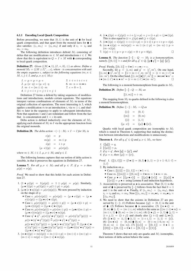
6.1.1 Encoding Local Quark CompositionBefore proceeding, we note that 〈0, 1〉 is the unit of � for localquark composition, and that apart from the monoid laws for � italso satisfies: 〈i1,m1〉 = 〈i2,m2〉 if and only if i1 = i2 andm1 = m2.

The following definition introduces deltoid MI consisting ofdeltas that are modifications m ∈ M and introductions i ∈ I . Weshow that this is equivalent to Q = I ×M with � correspondingto local quark composition.

Definition 27. Given ((M, •, 1), (I,+, 0),�) as above. Define amonoid MI = ((M ∪ I)∗, ·, ε), where · is concatenation with unitthe empty sequence ε, subject to the following equations (m,n ∈M , i, j ∈ I , and µ, ν, η ∈MI ):

1. ε ·µ = µ = µ · ε2. µ ·(ν · η) = (µ · ν) · η3. m · i = (m� i) ·m4. i · j = i+ j = j + i = j · i

5. i · i = i+ i = i6. m ·n = m • n7. ε = 0 = 1.

Definition 27 forms a deltoid by taking sequences of modifica-tions and introductions, modulo certain equations. The equationsinterpret various combinations of elements of MI in terms of theoriginal collection of operations. The most interesting is 3, whichapplies a modification m to an introduction i, via m� i, and shuf-fles m later in the sequence to apply to subsequent introductions.Note that equations 1 and 2 are redundant and follow from the factthat · is concatenation and 1 = ε its unit.

Delta action is defined inductively over the elements of MI ,applying each element ofMI to I via the appropriate function fromthe original monoids.

Definition 28. The delta action −(−) : MI × I → I for MI is

ε(p) = p

m(p) = m� pi(p) = i+ p

(µ · ν)(p) = µ(ν(p)).

where m ∈M , i ∈ I , µ, ν ∈MI and p ∈ I .

The following lemma captures that our notion of delta action issensible, in that it preserves the equations in Definition 27.

Lemma 7. For all µ, ν ∈ MI and all p ∈ P , if µ = ν thenµ(p) = ν(p).

Proof. We need to show that this holds for each axiom in Defini-tion 27.

1. (1 • µ)(p) = 1(µ(p)) = 1 � µ(p) = µ(p). Similarly,(µ • 1)(p) = µ(1(p)) = µ(1� p) = µ(p).

2. (µ • (ν • η))(p) = µ(ν(η(p))). We now proceed by inductionon the shape of η:• Case ε. µ(ν(ε(p))) = µ(ν(p)) = (µ • ν)(p) = (µ •ν)(ε(p)) = ((µ • ν) • ε)(p).• Case i. µ(ν(i(p))) = µ(ν(i+ p)) = (µ • ν)(i+ p) =

(µ • ν)(i(p)) = ((µ • ν) • i)(p).• Casem. µ(ν(m(p))) = µ(ν(m� p)) = (µ•ν)(m� p) =

(µ • ν)(m(p)) = ((µ • ν) •m)(p).• Case η′ • η′′. µ(ν((η′ • η′′)(p))) = µ(ν(η′(η′′(p)))) =

µ((ν • (η′ • η′′))(p)) ih= µ((ν • η′) • η′′)(p)) =

µ((ν • η′)(η′′(p))) = (µ • (ν • η′))(η′′(p)) ih= ((µ • ν) •

η′)(η′′(p)) = ((µ•ν)(η′(η′′(p))) = ((µ•ν)((η′ • η′′)(p)) =((µ • ν) • (η′ • η′′)(p).

3. (m • i)(p) = m(i(p)) = m� (i+ p) = (m� i) + (m� p) =(m� i) +m(p) = ((m� i) •m)(p).

4. (i • j)(p) = i(j(p)) = i+ (j+ p) = j+ (i+ p) = (j • i)(p).This is also equal to (i+ j)(p) and (j + i)(p).

5. (i• i)(p) = i(i(p)) = i+(i+p) = (i+ i)+p = i+p = i(p).6. (m • n)(p) = m(n(p)) = m � (n � p) = (m ·n) � p =

(m ·n)(p).7. 1(p) = 1� p = p = ε(p) = 0 + p = 0(p).

Lemma 8. The function J−K : Q → MI is a homomorphism,namely, J〈0, 1〉K = ε and for all q, q′ ∈ Q, Jq � q′K = JqK ·Jq′K.

Proof. Firstly, J〈0, 1〉K = 0 • 1 = ε • ε = ε.Secondly, let q = 〈i,m〉 and q′ = 〈i′,m′〉. On one hand,

J〈i,m〉� 〈i′,m′〉K = J〈i+m� i′,m ·m′〉K = (i + m � i′) •(m ·m′). On the other hand, J〈i,m〉K•J〈i′,m′〉K = i•m•i′•m′ =i • (m� i′) •m •m′ = (i+m� i′) • (m ·m′).

The following is a monoid homomorphism from quarks to MI .

Definition 29. Define J−K : Q→MI as

J〈i,m〉K = i ·m.The mapping fromMI to quarks defined in the following is also

a monoid homomorphism.

Definition 30. Define 〈〈−〉〉 : MI → Q as

〈〈ε〉〉 = 〈0, 1〉〈〈m〉〉 = 〈0,m〉〈〈i〉〉 = 〈i, 1〉

〈〈µ · ν〉〉 = 〈〈µ〉〉� 〈〈ν〉〉.Quarks with local quark composition are isomorphic to MI

which is stated in Theorem 4, supporting that making the distinc-tion between introductions and modifications is unnecessary.

Theorem 4. For all q, q′ ∈ Q and µ, ν ∈MI , we have

1. 〈〈JqK〉〉 = q,2. J〈〈µ〉〉K = µ,3. if q = q′, then JqK = Jq′K, and4. if µ = ν, then 〈〈µ〉〉 = 〈〈ν〉〉.

Proof. 1. 〈〈J〈i, l〉K〉〉 = 〈〈l • i〉〉 = 〈0, l〉� 〈i, 1〉 = 〈i+ 1 · 0, 1 · l〉 =〈i, l〉

2. By induction on µ.• Case i. J〈〈i〉〉K = J〈i, 1〉K = i • 1 = i.• Case m. J〈〈m〉〉K = J〈0,m〉K = 0 •m = 1 •m = m.• Case µ • ν: J〈〈µ • ν〉〉K = J〈〈µ〉〉� 〈〈ν〉〉K = J〈〈µ〉〉K •

J〈〈ν〉〉K = µ • ν. using Lemma 8 and induction hypothesis.3. Associativity is preserved as • is associative. That 〈0, 1〉 is the

unit of � is preserved by J−K follows from the fact that 0 = 1and 1 is the unit of •. Finally, if 〈i1,m1〉 = 〈i2,m2〉, theni1 = i2 andm1 = m2. Now J〈i1,m1〉K = m1•i1 = m2•i2 =J〈i2,m2〉K.

4. We need to show that the axioms in Definition 27 are pre-served by 〈〈−〉〉. (1) Follows because 〈〈q〉〉 = 〈0, 1〉 is the unitof �. (2) Follows because � is associative. (3) 〈〈m • i〉〉 =〈0,m〉� 〈i, 1〉 = 〈m� i,m〉which is the same as 〈〈(m� i) •m〉〉 =〈m� i, 1〉� 〈0,m〉 = 〈m� i,m〉. (4) 〈〈i • j〉〉 = 〈i, 1〉� 〈j, 1〉 =〈i+ j, 1〉 = 〈〈i+ j〉〉 and clearly also 〈〈j + i〉〉 and 〈〈j • i〉〉.(5) 〈〈i • i〉〉 = 〈i, 1〉� 〈i, 1〉 = 〈i+ i, 1〉 = 〈i, 1〉 = 〈〈i〉〉.(6) 〈〈m • n〉〉 = 〈0,m〉� 〈0, n〉 = 〈0 +m� 0,m ·n〉 =〈0,m ·n〉 = 〈〈m ·n〉〉. (7) J〈〈ε〉〉K = J〈0, 1〉K = 0 • 1 =J〈〈0〉〉K = J〈0, 1〉K = 0 • 1 = J〈0, 1〉K = J〈〈1〉〉K.

Theorem 5 shows that not only are quarks and MI isomorphic,their notions of delta action behave the same.

11 2010/8/9

Theorem 5. For all q ∈ Q and all p ∈ I ,

image(q � 〈p, 1〉) = JqK(p)and for all µ ∈MI and all i ∈ I ,

image(〈〈µ〉〉� 〈p, 1〉) = µ(p).

Proof. Firstly, image(〈i,m〉� 〈p, 1〉) = image(〈i+ (m� p),m〉) =i+(m�p) and J〈i,m〉K(p) = (i•m)(p) = i(m(p)) = i+(m�p).

Secondly, we prove by induction using the hypothesis for allµ ∈ MI and all i ∈ I , there exists an m such that 〈〈µ〉〉� 〈p, 1〉 =〈µ(p),m〉, which clearly implies the desired result. Proceed byinduction on form of µ:

• Case i. 〈〈i〉〉� 〈p, 1〉 = 〈i, 1〉� 〈p, 1〉 = 〈i+ p, 1〉. Now i(p) =i+ p, as desired.• Case m. 〈〈m〉〉� 〈p, 1〉 = 〈0,m〉� 〈p, 1〉 = 〈m� p,m〉. Nowm(p) = m� p, as desired.• Case µ • ν. 〈〈µ • ν〉〉� 〈p, 1〉 = 〈〈µ〉〉� 〈〈ν〉〉� 〈p, 1〉. By in-

duction hypothesis, there exists an m such that 〈〈ν〉〉� 〈p, 1〉 =〈ν(p),m〉. Similarly, applying the induction hypothesis to µ ∈MI and 〈ν(p),m〉 ∈ P , we obtain that there exists an n suchthat 〈〈µ〉〉� 〈ν(p),m〉 = 〈µ(ν(p)), n〉. By Definition 27(deltaaction) this equals 〈(µ • ν)(p), n〉, and we are done.

6.1.2 Encoding Batory and Smith’s Full Quark CompositionEncoding full quark composition is straightforward. To do so, weadapt the encoding above to use quarksQ = M×MI , where quarkcomposition is 〈m,µ〉� 〈n, ν〉 = 〈m • n, µ · ν〉 and define deltaapplication −(−) : Q × I → I to be 〈m,µ〉(p) = m � (µ(p)),relying on delta application for MI .

In the absence of other assumptions, this notion of delta appli-cation is not an action, as for example:

〈m,µ〉� 〈n, ν〉(p) = 〈m • n, µ · ν〉(p)= (m • n)� (µ · ν(p))

= (m • n)� (µ(ν(p)))

whereas

〈m,µ〉(〈n, µ〉(p)) = m� (µ(n� (ν(p))))

If we instantiate µ and ν with m′ and n′ we have in the first case:

(m • n)�m′(n′(p)) = (m • n)� (m′ � (n� p))= (m • n •m′ • n′)� p

and in the second case

m�m′(n� n′(p)) = m� (m′ � (n� (n′ � p)))= (m •m′ • n • n′)� p

which are equal in general only if • is commutative.

6.1.3 Encoding Batory and Smith’s Modifiers of ModifiersEncoding modifiers of modifiers is also straightforward. We as-sume that such modifiers, h : M → M , are endomorphismson the monoid of modifications (this is already implicit in Batoryand Smith’s Rh function): that is, h(1) = 1 and h(m2 • m1) =h(m2) • h(m1), for all m1,m2 ∈M .

We can extend the previous example to apply higher-order mod-ifiers to the global modifications as follows:

• quarks:Q = (M →M)×M×MI — a modifier of modifiers,a global modification, and a delta• composition: 〈h2, g2, µ2〉� 〈h1, g1, µ1〉 = 〈h2, g2, µ2 ·µ1〉,

and• delta application is 〈h, g, µ〉(p) = h(g)� (µ(p)).

To modify this definition so that h applies also to the localmodifications requires lifting h : M → M to hI : MI → MI ,defined by the following equation:

h(m� i) = h(m)� i.where h(i) = h(1 · i) = h(1� i) = h(1)� i = 1� i = i. In thiscase the delta application becomes

〈h, g, µ〉(p) = h(g)� (h(µ)(p)).

Again delta application is not an action, for the same reason asfor full quark composition.

Apel et al. [4] give the signatures of an entire hierarchy ofmodifiers of modifiers, but provide no further details.

6.2 Darcs and Patch TheoryThe version control system Darcs is formalised in terms of patchtheory [18]. The underlying formalism has some similarities withour work. Most notable is that ‘patches’ are modeled using a semi-group with inverses. This structure is a monoid at heart, with addi-tional properties (such as inverses) that do not entirely make sensein our setting. The most significant similarity is that they deal withconflictors (entities for resolving conflicts), which are similar toour conflict resolving deltas. Conflictors have a more complex setof properties than our conflict resolving deltas due to the addedstructure of their core setting. Patch theory should nonetheless of-fer inspiration to guide future research.

7. Related WorkIn general, approaches to facilitating automated product genera-tion for software product lines can be classified in two main di-rections [22]. Firstly, annotative approaches, such as conditionalcompilation, frames [44] or COLORED FEATHERWEIGHT JAVA(CFJ) [20], mark a model of the complete product line with respectto product features and remove marked product parts to obtain aproduct for a particular feature configuration.

Secondly, compositional approaches, such as delta model-ing [37–39], associate product fragments to product features, whichare assembled to implement a particular feature configuration. Aprominent example of this approach is AHEAD [7], which canbe applied on the design as well as on the implementation level.In AHEAD, a product is built by stepwise refinement of a basemodule with a sequence of feature modules. Design-level modelscan also be constructed using aspect-oriented composition tech-niques [16, 30, 43]. Apel et al. [36] apply model superpositionto compose model fragments. Perrouin et al. [33] obtain a prod-uct model by model composition and subsequently refinement bymodel transformation. In Haugen et al. [15], a set of models isrepresented by a base model with associated variability and resolu-tion models determining how modeling elements of the base modelhave to be replaced for a particular product model.

On the programming language level, several program modular-ization techniques [26], such as aspects [21], framed aspects [27],mixins [40], hyperslices [41] or traits [9, 14], are used to im-plement features in a compositional fashion. In addition, themodularity concepts of recent languages, such as SCALA [31]or NEWSPEAK [10], can be used to represent product features.CeasarJ [29] and Aspectual Feature Modules [3] are proposed as acombination of feature modules and aspects to modularize cross-cutting concerns.

The notion of program deltas was introduced by Lopez-Herrejonet al. [26] to describe the modifications of object-oriented pro-grams. Schaefer et al. [39] introduced the concept of delta modelingas a means to develop product line artifacts suitable for automatedproduct derivation and implemented with frame technology [44].

12 2010/8/9

In subsequent work [37], delta modeling is extended to a seam-less model-based development approach for SPLs where an initialproduct line representation is stepwise refined until an implementa-tion can be generated. The conceptual ideas of delta modeling havealso been instantiated on the programming language level in an ex-tension of Java with core and delta modules allowing the automaticgeneration of Java-based product implementations [38].

Originally, the delta model of a product line consisted of a sin-gle core and a set of incomparable product deltas [37, 39]. Con-flicts between deltas applicable for the same feature configurationwere prohibited. In order to express all possible products, an ad-ditional delta covering the combination of the potentially conflict-ing deltas had to be specified leading to product fragments. Sub-sequently, a partial ordering between deltas was introduced [38].However, it was required that all conflicts were manually resolvedby specifying an appropriate ordering. In contrast, in this paper, amore flexible notion of conflicts and conflict resolution is proposedthat allows intermediate conflicts between deltas as long as theyare eliminated later in a derivation by a conflict-resolving delta.The notion of conflict-resolving deltas is similar to lifters [35] orderivatives [25] in feature-oriented programming which are used tofacilitate the correct interaction between different feature modules.

The definition of a conflict as a lack of commutativity betweenmodifications is also discussed in the context of program refactor-ing [28]. The underlying formalisation uses graph transformationsystems and critical pair analysis. Oldevik et al. [32] define a con-flict in a sequence of model transformations to occur if two trans-formations do not commute. A similar notion of conflict related tonon-commutativity is observed by Apel et. al. [5] when two aspectsadvise shared join points.

8. ConclusionDelta modeling is an approach to facilitating automated productderivation for software product lines. In this paper, we generalizedthe conceptual ideas of delta modeling in an abstract, algebraicsetting. The main contribution of this work is the novel treatmentof conflicts between deltas by explicit conflict-resolving deltas. Inorder to ensure that for every valid feature configuration a uniqueproduct is generated, a conflict-resolving delta has to exist forevery pair of conflicting deltas in the model. We presented efficientconditions that allow checking the unambiguity of a product linewithout requiring to generate all products.

For future work, we will be using the ideas of abstract deltamodeling for the implementation of variability within the HATSABS language [1]. In addition, we are planning to extend abstractdelta modeling with a concept of hierarchy so that a delta can itselfbe a delta model. This will give rise to a more modular developmenttechnique for product lines based on nested delta models. Finally,variants of abstract delta modeling, such as basing the frameworkon partial monoids with a partial composition operation, will beinvestigated.

References[1] Highly Adaptable and Trustworthy Software using Formal Methods

(HATS), March 2009. http://www.hats-project.eu.

[2] S. Apel, C. Kastner, and C. Lengauer. FeatureHouse: Language-independent, automated software composition. In ICSE, pages 221–231, 2009.

[3] S. Apel, T. Leich, and G. Saake. Aspectual feature modules. IEEETrans. Software Eng., 34(2):162–180, 2008.

[4] S. Apel, C. Lengauer, B. Moller, and C. Kastner. An algebraic founda-tion for automatic feature-based program synthesis. Science of Com-puter Programming (SCP), 2010. To appear.

[5] Sven Apel, Christian Kastner, and Don S. Batory. Program refactoringusing functional aspects. In GPCE, pages 161–170, 2008.

[6] D.S. Batory and S.W. O’Malley. The design and implementation ofhierarchical software systems with reusable components. ACM Trans.Softw. Eng. Methodol., 1(4):355–398, 1992.

[7] D.S. Batory, J. Sarvela, and A. Rauschmayer. Scaling Step-WiseRefinement. IEEE Trans. Software Eng., 30(6), 2004.

[8] D.S. Batory and D. Smith. Finite map spaces and quarks: Algebras ofprogram structure. Technical Report TR-07-66, University of Texas atAustin, Dept. of Computer Sciences, 2007.

[9] L. Bettini, F. Damiani, and I. Schaefer. Implementing Software Prod-uct Lines using Traits. In Proc. of Object-Oriented Programming Lan-guages and Systems (OOPS), Track of ACM SAC, 2010.

[10] G. Bracha. Executable Grammars in Newspeak. ENTCS, 193:3–18,2007.

[11] P. Clements and L. Northrop. Software Product Lines: Practices andPatterns. Addison Wesley Longman, 2001.

[12] K. Czarnecki and M. Antkiewicz. Mapping Features to Models: ATemplate Approach Based on Superimposed Variants. In Conf. onGenerative Programming and Component Engineering(GPCE), 2005.

[13] S. Deelstra, M. Sinnema, and J. Bosch. Product Derivation in SoftwareProduct Families: A Case Study. Journal of Systems and Software,74(2):173–194, 2005.

[14] S. Ducasse, O. Nierstrasz, N. Scharli, R. Wuyts, and A. Black. Traits:A mechanism for fine-grained reuse. ACM TOPLAS, 28(2), 2006.

[15] Ø. Haugen, B. Møller-Pedersen, J. Oldevik, G. Olsen, and A. Svend-sen. Adding Standardized Variability to Domain Specific Languages.In SPLC, 2008.

[16] F. Heidenreich and C. Wende. Bridging the Gap Between Features andModels. In Aspect-Oriented Product Line Engineering (AOPLE’07),2007.

[17] P. Heymans, P.Y. Schobbens, J.C. Trigaux, Y. Bontemps, R. Matulevi-cius, and A. Classen. Evaluating formal properties of feature diagramlanguages. Software, IET, 2(3):281–302, 2008.

[18] J. Jacobson. A formalization of Darcs patch theory using inversesemigroups. Technical Report CAM report 09-83, UCLA, 2009.

[19] Kyo C. Kang, S. Cohen, J. Hess, W. Nowak, and S. Peterson. Feature-Oriented domain analysis (FODA) feasibility study. Technical Re-port CMU/SEI-90-TR-021, Carnegie Mellon University Software En-gineering Institute, 1990.

[20] C. Kastner and S. Apel. Type-Checking Software Product Lines - AFormal Approach. In ASE, pages 258–267. IEEE, 2008.

[21] C. Kastner, S. Apel, and D.S. Batory. A Case Study ImplementingFeatures Using AspectJ. In SPLC, pages 223–232. IEEE, 2007.

[22] C. Kastner, S. Apel, and M. Kuhlemann. Granularity in softwareproduct lines. In ICSE, pages 311–320, 2008.

[23] C. Kastner, S. Apel, S.S. ur Rahman, M. Rosenmuller, D. Batory, andG. Saake. On the impact of the optional feature problem: Analysis andcase studies. In Proc. Int’l Software Product Line Conference (SPLC).SEI, 2009.

[24] C.W. Krueger. New Methods in Software Product Line Development.In SPLC, pages 95–102, 2006.

[25] Jia Liu, Don S. Batory, and Christian Lengauer. Feature orientedrefactoring of legacy applications. In ICSE, pages 112–121, 2006.

[26] R.E. Lopez-Herrejon, D.S. Batory, and W.R. Cook. Evaluating Sup-port for Features in Advanced Modularization Technologies. InECOOP, volume 3586 of LNCS, pages 169–194. Springer, 2005.

[27] N. Loughran and A. Rashid. Framed aspects: Supporting variabilityand configurability for AOP. In ICSR, volume 3107 of LNCS, pages127–140. Springer, 2004.

[28] Tom Mens, Gabriele Taentzer, and Olga Runge. Detecting structuralrefactoring conflicts using critical pair analysis. Electr. Notes Theor.Comput. Sci., 127(3):113–128, 2005.

13 2010/8/9

[29] M. Mezini and K. Ostermann. Variability management with feature-oriented programming and aspects. In SIGSOFT FSE, pages 127–136.ACM, 2004.

[30] N. Noda and T. Kishi. Aspect-Oriented Modeling for VariabilityManagement. In SPLC, 2008.

[31] M. Odersky. The Scala Language Specification, version 2.4. Technicalreport, Programming Methods Laboratory, EPFL, 2007.

[32] Jon Oldevik, Øystein Haugen, and Birger Møller-Pedersen. Conflu-ence in domain-independent product line transformations. In FASE,pages 34–48, 2009.

[33] G. Perrouin, J. Klein, N. Guelfi, and J.-M. Jezequel. ReconcilingAutomation and Flexibility in Product Derivation. In SPLC, 2008.

[34] K. Pohl, G. Bockle, and F. Van Der Linden. Software Product LineEngineering: Foundations, Principles, and Techniques. Springer, Hei-delberg, 2005.

[35] Christian Prehofer. Feature-oriented programming: A fresh look atobjects. In ECOOP, volume 1241 of LNCS, pages 419–443. Springer,1997.

[36] S. Trujillo S. Apel, F. Janda and C. Kastner. Model Superimpositionin Software Product Lines. In International Conference on ModelTransformation (ICMT), 2009.

[37] I. Schaefer. Variability Modelling for Model-Driven Development ofSoftware Product Lines. In Intl. Workshop on Variability Modelling ofSoftware-intensive Systems (VaMoS 2010), 2010.

[38] I. Schaefer, L. Bettini, V. Bono, F. Damiani, and N. Tanzarella. Delta-oriented programming of software product lines. In Proceedings,14th International Software Product Line Conference, Lecture Notesin Computer Science, Jeju, South Korea, 2010. Springer. To appear.

[39] I. Schaefer, A. Worret, and A. Poetzsch-Heffter. A Model-BasedFramework for Automated Product Derivation. In Proc. of Workshopin Model-based Approaches for Product Line Engineering (MAPLE2009), 2009.

[40] Y. Smaragdakis and D.S. Batory. Mixin layers: an object-oriented im-plementation technique for refinements and collaboration-based de-signs. ACM Trans. Softw. Eng. Methodol., 11(2):215–255, 2002.

[41] P. Tarr, H. Ossher, W. Harrison, and S.M Sutton Jr. N degrees ofseparation: multi-dimensional separation of concerns. In ICSE, pages107–119, 1999.

[42] A. van Deursen and P. Klint. Domain-specific language design re-quires feature descriptions. Journal of Computing and InformationTechnology, 10(1):1–18, 2002.

[43] M. Volter and I. Groher. Product Line Implementation using Aspect-Oriented and Model-Driven Software Development. In SPLC, pages233–242, 2007.

[44] H. Zhang and S. Jarzabek. An XVCL-based Approach to SoftwareProduct Line Development. In Software Engineering and KnowledgeEngineering, pages 267–275, 2003.

14 2010/8/9