Efficiently Indexing Shortest Paths by ExploitingSymmetry in Graphs∗

Yanghua Xiao† Wentao Wu† Jian Pei‡ Wei Wang† Zhenying He††Department of Computing and Information Technology, Fudan University, Shanghai, China{shawyh, weiwang1, zhenying}@fudan.edu.cn, {wentaowu1984}@gmail.com

‡School of Computing Science, Simon Fraser University, Burnaby, BC, Canadajpei@cs.sfu.ca

ABSTRACTShortest path queries (SPQ) are essential in many graphanalysis and mining tasks. However, answering shortestpath queries on-the-fly on large graphs is costly. To onlineanswer shortest path queries, we may materialize and in-dex shortest paths. However, a straightforward index of allshortest paths in a graph of N vertices takes O(N2) space.In this paper, we tackle the problem of indexing shortestpaths and online answering shortest path queries. As manylarge real graphs are shown richly symmetric, the centralidea of our approach is to use graph symmetry to reduce theindex size while retaining the correctness and the efficiencyof shortest path query answering. Technically, we developa framework to index a large graph at the orbit level in-stead of the vertex level so that the number of breadth-firstsearch trees materialized is reduced from O(N) to O(|∆|),where |∆| ≤ N is the number of orbits in the graph. Weexplore orbit adjacency and local symmetry to obtain com-pact breadth-first-search trees (compact BFS-trees). An ex-tensive empirical study using both synthetic data and realdata shows that compact BFS-trees can be built efficientlyand the space cost can be reduced substantially. Moreover,online shortest path query answering can be achieved usingcompact BFS-trees.

1. INTRODUCTIONShortest path queries (SPQ) are essential in many graph

∗The work was supported in part by the National NaturalScience Foundation of China under Grants No. 60673133 andNo. 60703093, the National Grand Fundamental Research973 Program of China under Grant No. 2005CB321905,Shanghai Leading Academic Discipline Project UnderProject No. B114, a Natural Sciences and Engineering Re-search Council of Canada (NSERC) Discovery grant, anda Natural Sciences and Engineering Research Council ofCanada (NSERC) Discovery Accelerator Supplements grant.All opinions, findings, conclusions and recommendations inthis paper are those of the authors and do not necessarilyreflect the views of the funding agencies.

Permission to copy without fee all or part of this material is granted pro-vided that the copies are not made or distributed for direct commercial ad-vantage, the ACM copyright notice and the title of the publication and itsdate appear, and notice is given that copying is by permission of the ACM.To copy otherwise, or to republish, to post on servers or to redistribute tolists, requires a fee and/or special permissions from the publisher, ACM.EDBT 2009, March 24–26, 2009, Saint Petersburg, Russia.Copyright 2009 ACM 978-1-60558-422-5/09/0003 ...$5.00

v1

v10

v3 v4

v8v7

v6v5

v9

v2

Figure 1: Graph G as our Running example

analysis and mining tasks. For example, in metabolic net-work analysis, for a given pair of compounds, the shortestpathway is particularly interesting [19]. In a large communi-cation network, the shortest paths are important for systemresource management [18, 5]. Moreover, shortest paths arealso important in characterizing the internal structure of alarge graph [27, 23].

Answering shortest path queries on-the-fly on large graphsis costly. To find the shortest path between a pair of ver-tices u and v, a straightforward approach is to start a recur-sive breadth-first search from u until v is reached. Such astraightforward method has time complexity O(N + M) ona graph of N vertices and M edges [9].

To achieve online shortest path query answering, a materi-alization approach is to pre-compute and index the shortestpaths between every pair of vertices in a large graph offlineso that any shortest path queries can be answered online inalmost constant time. In an undirected graph of N vertices,there are N(N −1)/2 pairs of vertices and thus at least thatmany shortest paths. A straightforward implementation ofthe materialization strategy takes O(N2) space. For largegraphs, the space cost is often a critical concern.

In this paper, we tackle the problem of indexing short-est paths and online answering shortest path queries. Theobjective is to reduce the space cost of the indexes and si-multaneously achieve online shortest path query answering.Our method is motivated by the fact that symmetry exten-sively exists in large graphs [11, 29, 30, 28]. While we willreview the formal definition of graph symmetry in Section 2,let us illustrate the intuition using an example.

Example 1 (Symmetry). Consider graph G in Fig-ure 1. Vertices v1 and v2 have the following property: forany vertex v ∈ (V (G)− {v1, v2}), the shortest path betweenv1 to v and the shortest path between v2 to v differ only onedges (v1, v3) and (v2, v3). As will be shown in Section 2, thisproperty can be captured by an automorphic equivalence rela-

493

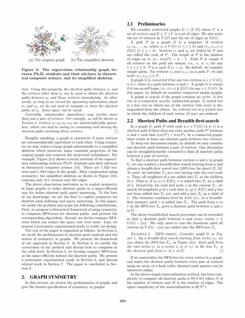
(a) The original graph (b) The simplified skeleton

Figure 2: The supervision relationship graph be-tween Ph.D. students and their advisors in theoret-ical computer science, and its simplified skeleton.

tion. Using this property, the shortest paths between v1 andthe vertices other than v2 can be used to obtain the shortestpaths between v2 and those vertices immediately. In otherwords, as long as we record the symmetry information aboutv1 and v2, we do not need to compute or store the shortestpaths of v2. Some space can be saved.

Generally, automorphic equivalence may involve morethan just a pair of vertices. For example, as will be shown inSection 2, vertices v7, v8, v9, v10 are automorphically equiva-lent, which can lead to saving in computing and storing theshortest paths involving those vertices.

Roughly speaking, a graph is symmetric if some verticesare automorphically equivalent to each other. Using symme-try we may reduce a large graph substantially to a simplifiedskeleton which preserves many essential properties of theoriginal graph and removes the structural redundancy. Forexample, Figure 2(a) shows a social network of the supervi-sion relationship between Ph.D. students and their advisorsin theoretical computer science [14]. There are 1, 025 ver-tices and 1, 043 edges in the graph. After compression usingsymmetry, the simplified skeleton as shown in Figure 2(b)contains only 511 vertices and 525 edges.

The above observation motivates us to exploit symmetryin large graphs to index shortest paths in a space-efficientway for online shortest path query answering. To the bestof our knowledge, we are the first to exploit symmetry forshortest path indexing and query answering. In this paper,we tackle the problem and make the following contributions.First, we propose a theoretical framework of using symmetryto compress BFS-trees for shortest paths, and present thecorresponding algorithms. Second, we devise compact BFS-trees which can reduce the space cost even more. Last, wepresent a systematic experimental study to verify our design.

The rest of the paper is organized as follows. In Section 2,we recall the preliminaries in shortest path analysis and thenotion of symmetry in graphs. We present the frameworkof our approach in Section 3. In Section 4, we justify thecorrectness of our method and discuss how to compress atthe orbit level. In Section 5, we develop compact BFS-treesas the space-efficient indexes for shortest paths. We presenta systematic experimental study in Section 6, and discussrelated work in Section 7. The paper is concluded in Sec-tion 8.

2. GRAPH SYMMETRYIn this section, we review the preliminaries of graphs and

give the formal specification of symmetry in graphs.

2.1 PreliminariesWe consider undirected graphs G = (V, E) where V is a

set of vertices and E ⊆ V ×V is a set of edges. We also writethe set of vertices as V (G) and the set of edges as E(G).

A path P in a graph G is a sequence of verticesv1, v2, . . . , vk, where vi ∈ V (G) (1 ≤ i ≤ k) and (vj , vj+1) ∈E(G) (1 ≤ j < k). Vertices v1 and vk are linked by P andare called the ends of P . The length of P is the numberof edges on it, i.e., len(P ) = k − 1. Path P is simple ifall vertices on the path are unique, i.e., vi 6= vj for any1 ≤ i, j ≤ k. P is a cycle if v1 = vk. By default, we considersimple paths. For vertices vj and vj+1 on a path P , we alsowrite (vj , vj+1) ∈ P .

A graph G is connected if for any two vertices u, v ∈ V (G),u 6= v, there is a path between u and v. A graph G is simpleif it has no self loops, i.e., (v, v) 6∈ E(G) for any v ∈ V (G). Inthis paper, by default we consider connected simple graphs.

A graph is acyclic if the graph contains no cycle. A freetree is a connected, acyclic, undirected graph. A rooted treeis a free tree in which one of the vertices (the root) is dis-tinguished from the others. An ordered tree is a rooted treein which the children of each vertex (if any) are ordered.

2.2 Shortest Paths and Breadth-first-searchIn a graph G, path P with ends u, v ∈ V (G) (u 6= v) is a

shortest path if there does not exist another path P ′ betweenu and v such that len(P ′) < len(P ). In a connected graph,there exists at least one shortest path between two vertices.

To keep our discussion simple, by default we only considerone shortest path between a pair of vertices. Our discussioncan be straightforwardly extended to find all shortest pathsbetween a pair of vertices.

To find a shortest path between vertices u and v in graphG, we can conduct a breadth-first search starting from u andobtain a breadth-first search tree (BFS-tree for short) Tu [9].To start, we initialize Tu as a tree having only the root nodeu. Then, all neighbors of u are added into Tu as the childrenof u. That is, if (u, x) ∈ E(G), x is added into Tu as a childof u. Iteratively, for each leaf node x in the current Tu, wesearch all neighbors y of x such that (x, y) ∈ E(G) and y hasnot been added into Tu yet, and add y into Tu as a child ofx. The iteration continues level by level (i.e., in a breadth-first manner) until v is added into Tu. The path from u tov in the BFS-tree Tu gives a shortest path between u and vin G.

The above breadth-first search procedure can be extendedto find a shortest path between u and every vertex v ∈V (G) − {u}. We only need to run the iterations until allvertices in V (G)− {u} are added into the BFS-tree Tu.

Example 2 (BFS-trees). Consider graph G in Fig-ure 1. By a breadth-first search starting from vertex v1, wecan obtain the BFS-tree Tv1 in Figure 3(a). Each path fromthe root vertex v1 to a vertex x (x 6= v1) in the tree Tv1 isthe shortest path from v1 to x in G.

If we materialize the BFS-tree for every vertex in a graph,and index the shortest paths between every pair of verticesusing an array or a hash table, shortest path queries can beanswered online.

In the above simple materialization method, the time com-plexity to compute all shortest paths is Θ(NM) where N isthe number of vertices and M is the number of edges. Thespace complexity of the materialization is Θ(N2).

494

v1

v10

v3

v4

v8v7

v6v5

v9

v2

v2

v10

v3

v4

v8v7

v6v5

v9

v1

g1=(v1,v2)

(a) Tv1 and Tv2

v1

v3

v2

v8v7

v6v5

v9

v4

v10

(b) Tv3

v1 v2

v3

v4

v8v7

v6v5

v9 v10

(c) Tv4

v1 v2

v3v4 v8v7

v6

v5

v9 v10

g2=(v5,v6)(v7,v9)(v8,v10)

v1 v2

v3v4 v10v9

v5

v6

v7 v8

(d) Tv5 and Tv6

v1 v2

v3 v4 v8

v7

v6

v5

v9 v10

g3=(v7,v8)

v1 v2

v3 v4 v7

v8

v6

v5

v9 v10

(e) Tv7 and Tv8

Figure 3: BFS-trees

2.3 Symmetry in GraphsGraph symmetry is an important topic in algebraic graph

theory [4, 12]. Here, we review some basic concepts.For graph G = (V, E), a permutation f : V 7→ V acting

on V is a bijective mapping from V onto itself. For a ver-tex u ∈ V , f maps u to vertex uf . Obviously, the inversecorrespondence f−1 of f is also a permutation.

Let S(V ) be the set of all permutations acting on V . Forpermutations f, g ∈ S(V ), the product h = f ◦ g (or simplyfg) is the mapping h : V 7→ V such that for each u ∈ V ,uh = (uf )g. Apparently, the product of two permutations isalso a permutation, i.e., f ◦ g ∈ S(V ).

Let f ∈ S(V ). The action of f on V can be extended toan induced action on V × V as follows: for (a, b) ∈ V × V ,we define (a, b)f = (af , bf ). For the set of edges E ⊆ V ×V ,we define Ef = {(a, b)f |(a, b) ∈ E}. If Ef = E, we call f anautomorphism of E.

Let Aut(G) be the set of all automorphisms of a graphG = (V, E). Mathematically, (Aut(G), V ) is a permutationgroup. In general, a graph G is asymmetric if (Aut(G), V )contains no permutations other than the identity permuta-tion e (i.e., ue = u for all vertices u). Otherwise, the graphis symmetric.

Automorphism group (Aut(G), V ) defines a relation=Aut(G) on V as follows. For two vertices u, v ∈ G,u =Aut(G) v if there exists an automorphism f ∈ Aut(G)

such that uf = v. Due to the identity permutation e ∈Aut(G), relation =Aut(G) is reflexive. Since uf = v im-

plies vf−1= u, relation =Aut(G) is symmetric. Moreover, if

xf = y and yg = z, xfg = z. Thus, relation =Aut(G) is tran-sitive. Therefore, =Aut(G) is an equivalence relation, and isusually called automorphic equivalence.

We can partition the set V (G) using equivalence relation=Aut(G). Let ∆(G) = V (G)/ =Aut(G) = {∆1, ∆2, . . . , ∆k}.That is, u, v ∈ ∆i (1 ≤ i ≤ k) if u =Aut(G) v. ∆(G) iscalled the automorphism partitioning. An entry ∆i ∈ ∆(G)is called an orbit of Aut(G). An orbit is trivial if it containsonly one vertex. Otherwise, the orbit is non-trivial. We alsowrite ∆(G) as ∆ when G is clear from context.

Orbits are important in our study. A non-trivial orbit cap-tures the set of vertices which can be compressed in shortestpath computation. We will discuss the details in the later

sections.In Aut(G), a subset F = {f1, . . . , fk} ⊆ Aut(G) is a set of

generators if every permutation f ∈ Aut(G) can be writtenas a product of some permutations in F , but for every propersubset F ′ of F , there exists at least one permutation f ∈Aut(G) such that f cannot be written as a product of somepermutations in F ′.

Let f be a permutation acting on vertex set V (G) of graphG(V, E). The support of permutation f is the set of verticesthat f moves, that is, supp(f) = {v ∈ V (G)|vf 6= v}. Apermutation is usually written as a union of some disjointcycles. For example, f = (a, b, c)(d, e) means af = b, bf =c, cf = a and df = e, ef = d. In the cycle representation, allvertices that f does not move are omitted.

Two permutations f and g are disjoint if their supportsare exclusive, i.e., supp(f) ∩ supp(g) = ∅. Moreover, twosets of permutations F1 and F2 are support-disjoint if forany f ∈ F1 and g ∈ F2, f and g are disjoint.

For a non-identity automorphism f ∈ Aut(G) (f 6= e), iff = f1f2 (f1, f2 ∈ Aut(G), supp(f1) ∩ supp(f2) = ∅) impliesf1 = e or f2 = e, then f is indecomposable. Otherwise,f is decomposable. In other words, an indecomposable au-tomorphism cannot be rewritten as a product of disjointnon-identity permutations, and thus can be considered asredundancy-free.

Example 3 (Concepts). For graph G in Figure 1,we can find a set of generators of Aut(G) consistingof the following automorphisms g1 = (v1, v2), g2 =(v5, v6)(v7, v9)(v8, v10), g3 = (v7, v8), and g4 = (v9, v10).

Due to g2, we have v7 =Aut(G) v9 and v8 =Aut(G) v10.Furthermore, due to g3, we have v7 =Aut(G) v8. Conse-quently, v7, v8, v9, v10 are in the same orbit of the graph.Given all the automorphisms, we can obtain the automor-phism partitioning of the graph ∆ = {∆1, ∆2, ∆3, ∆4, ∆5},where ∆1 = {v1, v2}, ∆2 = {v3}, ∆3 = {v4}, ∆4 = {v5, v6}and ∆5 = {v7, v8, v9, v10}. The automorphism partitioningis consistent with our observations in Example 1.

It is easy to check that supp(g1) = {v1, v2}, supp(g3) ={v7, v8} and supp(g2) = {v5, v6, v7, v8, v9, v10}. Hence, g1

and g3 are disjoint, but g2 is not disjoint with respect to g1

or g3. g1g3 = (v1, v2)(v7, v8) is decomposable since it is theproduct of two disjoint non-identity automorphisms g1 andg3. However, g1, g2, g3 and g4 are indecomposable.

495

Table 1: Automorphism StorageOrbit Base vertex Mirrored vertex and automorphism∆1 v1 〈v2, g1〉∆4 v5 〈v6, g2〉∆5 v7 〈v8, g3〉, 〈v9, g2〉, 〈v10, g3g2〉

Algorithm 1: The framework

Input: a graph G;Output: T: A set of compact BFS-trees;Obtain symmetry information and partition V (G) into1

orbits;foreach non-trivial orbit ∆i do2

select a base vertex u ∈ ∆i and compute the3

automorphisms fu,u′ for all u′ ∈ ∆i and u′ 6= u;

end4

conduct a breadth-first search to build the compact5

BFS-trees for the base vertices of all orbits;

3. THE FRAMEWORKAs indicated in Example 3, vertices v1 and v2 in graph

G in Figure 1 are in the same orbit. Figure 3(a) shows theBFS-trees of v1 and v2. Interestingly, the two BFS-treescan be mapped to each other under the action of automor-phism g1 = (v1, v2). Each path in Tv1 can be mapped to acorresponding path in Tv2 under the action of g1.

Generally, for vertices in the same orbit, their BFS-treescan be mapped to each other under an automorphism. Fig-ures 3(b), 3(c), 3(d) and 3(e) show more examples. Table 1shows the mapping automorphisms in the non-trivial obitsin graph G in Figure 1.

Based on the above observation, we can reduce the costof computing and storing shortest paths. For each orbit ∆,we select only one vertex u ∈ ∆ in the orbit as the basevertex, and generate the corresponding BFS-tree Tu. Forother vertices u′ ∈ ∆, we record the automorphism fu,u′

that maps the BFS-tree Tu to Tu′ .If a shortest path query involves at least one base vertex,

the query can be answered directly using the BFS-tree of thebase vertex. If both vertices u1 and v1 in a shortest pathquery are not the base ones, we can find the base vertexu of the orbit to which u1 belongs, and the shortest pathsbetween u and v1 in the BFS-tree Tu. The shortest pathsbetween u1 and v1 are given by applying the automorphismfu,u1 on those shortest paths between u and v1.

In this paper, we adopt the nice implementation innauty [17] to obtain the symmetry information including or-bits and a set of generators. The framework of our methodis shown in Algorithm 1.

4. ORBIT-BASED COMPRESSIONIn this section, we first justify the correctness of our

method. Then, we discuss how to compute automorphismsfor non-base vertices.

4.1 Shortest Paths Using OrbitsApparently, automorphisms have the following property

which enables us to find isomorphic subgraphs.

Lemma 1 (Automorphisms and subgraphs). LetH = (V ′, E′) be a subgraph of G = (V, E), i.e., V ′ ⊆ Vand E′ ⊆ E. For any automorphism f ∈ Aut(G),

Hf = (V ′f , E′f ) is a subgraph of G (i.e., V ′f ⊆ V andE′f ⊆ E) and isomorphic to H.

Moreover, automorphisms are significant for countingunique isomorphic copies of subgraphs. Let V ′ ⊆ V be asubset of vertices. The induced subgraph of V ′ is G(V ′) =(V ′, EV ′), where EV ′ = {(u, v) ∈ E|u, v ∈ V ′}.

Lemma 2. Consider graph G = (V, E) and a subset V ′ ⊆V . For an automorphism f ∈ Aut(G), if V ′f = V ′ thenG(V ′)f = G(V ′).

Proof. We only need to show E′f = E′. Since f ∈Aut(G) is an automorphism, E′f ⊆ E. For any edge(u, v) ∈ G(V ′), (u, v)f ∈ E′ due to V ′f = V ′. Hence,E′f ⊆ E ∩ V ′ × V ′ = E′. Since f is bijective, we haveE′f = E′, and thereby G(V ′)f = G(V ′).

An orbit captures a set of vertices which can be com-pressed due to symmetry. For a given graph G, how muchcan we compress? To understand this question, technicallywe need to explore, given an induced subgraph G(V ′) of G,how many unique isomorphic copies of G(V ′) exist in G.

For a graph G = (V, E) and a set of vertices Q ⊆ V ,an automorphism f ∈ Aut(G) is a setwise stabilizer withrespect to Q if Qf = Q, where Qf = {vf |v ∈ Q}. Wedenote the set of all setwise stabilizers with respect to Qby SS(G, Q). As shown in [24], SS(G, Q) is a subgroup ofAut(G). Moreover, we have the following result.

Theorem 1 (Compressibility). Let G = (V, E) be agraph, V ′ ⊆ V .

|G(V ′)Aut(G)| = |Aut(G)||SS(G, V ′)|

where G(V ′)Aut(G) = {G(V ′)f |f ∈ Aut(G)}.Proof. SS(G, V ′) is a subgroup of Aut(G) [24]. Thus,

the theorem is an immediate consequence of the Lagrange’sTheorem [20], which states that if H is a subgroup of P andP is a finite group then |P | = |H| · [P : H] where [P : H] isthe number of different cosets.

Theorem 1 indicates that the number of unique isomorphiccopies of G(V ′) depends on two factors, the size of Aut(G)and the setwise stabilizers with respect to V ′. One impor-tant intuition here is that a setwise stabilizer with respect toV ′ maps G(V ′) to itself and thus is redundant in subgraphenumeration.

Automorphisms also have the following nice property.

Lemma 3 (Shortest paths and automorphisms).Let P be a shortest path between vertices u and v in graphG. For any automorphism f ∈ Aut(G), P f is a shortestpath between uf and vf , where P f = {(xf , yf )|(x, y) ∈ P}.

Proof Sketch: Using Lemma 1, we can show that P f

is a path between uf and vf . Lauri and Scapellato [15]showed that automorphisms are geodesic-preserving. Thatis, d(u, v) = d(uf , vf ) where d(, ) is the geodesic dis-tance that measures shortest distance between a vertex pair.Therefore, len(P ) = len(P f ).

Assume that P is a shortest path between u and v. If P f

is not a shortest path between uf and vf , there must be a

shortest path P ′ which is shorter than P f . Clearly, P ′f−1

isa shorter path than P between u and v. Contradiction.

496

Now, we are ready to prove the correctness of our method.

Theorem 2 (BFS-trees and automorphisms). Forgraph G, let Tv be a BFS-tree rooted at vertex v ∈ V (G). Forany vertex u which is in the same orbit with v, there existsan automorphism f ∈ Aut(G) such that vf = u and T f

v is aBFS-tree rooted at vf , where T f

v = {(xf , yf )|(x, y) ∈ Tv} .Proof Sketch: Since u and v are in the same orbit, there

must exist at least one f ∈ Aut(G) such that u = vf . Now,we show T f

v is a BFS-tree rooted at u.According to Lemma 3, each path in T f

v is a shortest pathstarting from u = vf . For each vertex w ∈ V (G), a shortest

path between v and wf−1must appear in Tv. Let the path be

P . Then, P f is a path in T fv . Moreover, P f is a shortest

path between u and w.

Example 4 (BFS-trees and automorphisms). InFigure 3 and Table 1, T g1

v1 = Tv2 , T g2v5 = Tv6 , T g3

v7 = Tv8 ,T g2

v7 = Tv9 and T g3g2v7 = Tv10 .

4.2 Generating BFS-trees for an OrbitSection 4.1 shows that, in a non-trivial orbit ∆, we can

select one vertex v ∈ ∆ as the base vertex and generate theBFS tree. Any vertex in ∆ can serve as the base vertex.For other vertices u in the same orbit, we can find an auto-morphism f to map Tv to answer any shortest path queriesinvolving u. How can we find automorphisms for non-basevertices?

Example 5 (Choice of automorphisms). In ourrunning example (Figure 3 and Table 1), let us choose v1

as the base vertex in orbit ∆1. Two automorphisms g1 andg1g3 can map v1 to v2. In other words, the automorphismfor v2 is not unique. Which one is more preferable?

It is easy to see |supp(g1)| < |supp(g1g3)|. Hence, interms of storage cost, g1 is a better choice than g1g3.

In general, in an orbit ∆ where v is the base vertex, fora non-base vertex v′, there may exist more than one auto-morphism mapping v to v′. Let Gv→v′ = {f : vf = v′}be the set of automorphisms that map v to v′. Our task isto choose one automorphism from Gv→v′ for answering theshortest path queries for v′.

The cost of storing an automorphism f can be quantifiedas Θ(|supp(f)|). Therefore, it is desirable to use the auto-morphism f of the minimum |supp(f)| value. However, weconjecture that the following problem is NP-hard.

Conjecture 1 (Optimal automorphism selection).The following problem is NP-hard.Instance: a graph G(V, E), a positive number n, verticesv, v′ ∈ V .Question: is there an automorphism f ∈ Gv→v′ such that|supp(f)| ≤ n?

To tackle the problem in a practical way, we utilize a setof generators Gens of the automorphism group returnedby symmetry computation algorithm nauty [17]. Each au-tomorphism in Gens is indecomposable (part (1) of Theo-rem 2.34 in [17]), and thus can be regarded as redundancy-free. As will be shown in our experimental results, in prac-tice the storage cost of those automorphisms is very low.Thus, if one of those automorphisms can map the base ver-tex v to a non-base vertex v′, we use it for v′.

Algorithm 2: getAut(u,v,P)

Input: Two vertices u, vOutput: P: the set of automorphisms such that the

production of all automorphisms in P is anautomorphism mapping u to v

foreach p ∈ Gens do1

if up == v then2

P = P ∪ {p}; return true;3

end4

if !visited[up] then5

P = P ∪ {p}; visited[up] = true;6

if getAut(up, v,P) then7

return true;8

else9

P = P− {p}; visited[up] = false;10

end11

end12

end13

However, we may not be able to find an indecomposableautomorphism f ∈ Gv→v′ directly from Gens for a non-basevertex v′ such that vf = v′. In such a case, we have to searchthe possible products of the automorphisms in Gens. Theprocedure is shown in Algorithm 2.

Before calling the procedure, the variable visited for eachvertex is initialized to false except for vertex u. When weencounter an automorphism p such that up has been visited(which implies that the product of a segment of automor-phism sequence pi, pi+1, . . . , pj (pj = p) in P up = u), thesearch process along the current path can be terminated,since we can find a shorter automorphism sequence to trans-form vertex u to v.

Each possible product of the automorphisms in Gensleads to a candidate automorphism. Hence, Algorithm 2is exponential in the worst case. However, as shown in ourexperimental results, for real networks, in most cases we canfind the desirable automorphisms from Gens quickly.

Clearly, the total space cost to store the automorphismsfor non-based vertices is O((|V (G)|−|∆|)p), where |∆| is thenumber of orbits and p is the average support length of theautomorphisms for non-based vertices. Since each orbit hasonly one BFS-tree, the storage cost for BFS-trees is reducedfrom Θ(|V (G)|2) to Θ(|∆||V (G)|). Now, the last questionin this section is how we can estimate p and compare it tothe cost of storing a BFS-tree.

We say a graph G(V, E) to be globally symmetric if thereexists an indecomposable automorphism g ∈ Aut(G) suchthat supp(g) = V (G). Otherwise, we say the graph to belocally symmetric. It has been shown that real large graphsare unlikely globally symmetric [11]. Hence, the key is toquantify the degree to which a graph is locally symmetric.For this purpose, we define a measure ϕG as

ϕG =maxg∈ID(G){|supp(g)|}

|V (G)| ,

where ID(G) is the set of indecomposable automorphismsof graph G. Intuitively, the larger ϕG, the closer to globalsymmetric G is.

Example 6 (ϕG). In Figure 4(a), there exists an inde-composable automorphism f = (v1, v2)(v3, v4)(v5, v6)(v7, v8)

497

v1 v2

v3v4

v8v7

v6v5

(a) G1

v1 v2

v3 v4

v8v7

v6

v5

(b) G2

Figure 4: Local symmetry andglobal symmetry.

v1

v2

v3

v4 v5

v7

(a) Tv1

v1

v3

v4 v5

v7

(b) Tv3

v1

v3

v4

v5

v7

(c) Tv4

v1

v3

v4 v8v7

v6

v5

v9 v10

(d) Tv5

v1

v3 v4 v8

v7

v6

v5

v9 v10

(e) Tv7

Figure 5: compact BFS-trees

Table 2: Statistics of some real graphs (Avg and Max are the average orbit length and the maximal orbitlength, respectively)

Graph N |∆| rG% M ϕG‰ Avg MaxPPI 1458 1019 69.89 1948 4.11 1.43 46

Yeast 2284 1852 81.09 6646 2.63 1.23 34Homo 7020 6066 86.41 19811 0.57 1.15 44

P-fei1738 1738 1176 67.66 1876 5.75 1.48 10Geom 3621 2803 77.41 9461 1.66 1.29 13

Erdos02 6927 2365 34.14 11850 3.46 2.93 142DutchElite 3621 1907 52.67 4310 2.21 1.90 49

Eva 4475 898 20.07 4652 4.47 4.98 545California 5925 4009 67.66 15770 1.01 1.48 46

Epa 4253 2212 52.01 8897 0.94 1.92 115InternetAs 22442 11392 50.76 45550 0.27 1.97 343

moving all vertices, hence ϕG1 = 100% . In Figure 4(b),ϕG2 = 50% since g = (v1, v2)(v3, v4) is indecomposableand maximal in terms of cardinality of the support. No-tice that, automorphism h = (v1, v2)(v3, v4)(v7, v8) of G2

moves more vertices than g, however h is decomposable intothe composition of two disjoint automorphisms of G2: g andg′ = (v7, v8), thereby cannot be selected as the maximal oneto compute ϕG2 .

In Table 2, we give ϕG for a variety of real large graphs.Please refer to [28] for the details of each graph. It is evi-dent that real graphs are locally symmetric with the valueof ϕG at the order of magnitude of 10−3 or 10−4. Localsymmetry of real graphs implies that the automorphismsrequired to generate BFS-trees of non-base elements can bestored using very small storage space, thousands or tens ofthousands times smaller than storing a BFS-tree. More-over, the support of an automorphism in a graph G is atmost |V (G)| · ϕG. Thus, the storage cost of automorphismsis O((|V (G)| − |∆|)|V (G)|ϕG).

5. COMPACT BFS-TREESThe size of BFS-trees can be further reduced by utilizing

symmetry in a graph.

Example 7 (Compacting BFS-trees). In our run-ning example (Figure 1), ∆4 = {v5, v6} and ∆5 ={v7, v8, v9, v10}. Let us try to compact the BFS-trees Tv1 ,Tv3 and Tv4 in Figure 3 using the two orbits.

We can compact a BFS-tree such that only one vertex inan orbit is used as long as we can ensure the adjacency ofthe remaining vertices, as shown in Figure 5. It is easy tosee that the shortest path Pv1,v6 can be obtained from pathPv1,v5(under the action of g2). Moreover, the shortest paths

from v1 to v8, v9, v10, respectively, can be obtained from theshortest path Pv1,v7 under the action of g3, g2 and g3g2,respectively.

Not all orbits can be compacted in the above way. For ex-ample, in Tv7 , {v5, v6} cannot be compacted, since the lengthof the shortest path between v7 and v5 and that between v7

and v6 are different. Consequently, the shortest paths cannotbe mapped to each other under any automorphism.

In this section, we show that whether an orbit can becompacted in a BFS-tree is highly related to the reachabilityrelation between this orbit and the root orbit, the orbit towhich the root vertex belongs. We formulate our ideas usingorbit adjacency and orbit reachability. Then, we develop thecompact BFS-tree index structure and an efficient algorithmfor shortest path query answering using compact BFS-trees.

5.1 Orbit Adjacency and ReachabilityIf some vertex in orbit ∆i is adjacent to some vertex in

orbit ∆j , we say that orbits ∆i and ∆j are adjacent. Anorbit can be adjacent to itself. A sequence ∆1∆2 · · ·∆k oforbits is called as an orbit path if ∆i is adjacent to ∆i+1 foreach 1 ≤ i < k. If there is no repeated orbit in an orbitpath, we call the orbit path a simple orbit path.

Let ∆i and ∆j be two orbits in graph G. For vertexv ∈ ∆i, Nj(v) = {(u, v) ∈ E(G)|u ∈ ∆j} is the set ofneighbors of v that belong to orbit ∆j . Orbit ∆i is said tobe strongly adjacent to ∆j if for any two vertices v, v′ ∈ ∆i,Nj(v) = Nj(v

′).If there exists an orbit path ∆1∆2 · · ·∆k such that ∆i is

strongly adjacent to ∆i+1 for 1 ≤ i < k, we say that orbit∆1 is strongly reachable to orbit ∆k along the orbit path.

Lemma 4 (Strong adjacency). If orbit ∆i is

498

strongly adjacent to orbit ∆j, then for any vertex u in ∆i,Nj(u) = ∆j.

Proof. For any vertex u ∈ ∆i, Nj(u) ⊆ ∆j. Supposethere exists a vertex y ∈ ∆j but not in Nj(u), which impliesthat y will not be adjacent to any vertex in ∆i. Let x ∈Nj(u) be a vertex adjacent to vertex u ∈ ∆i. There mustexist some automorphism f ∈ Aut(G) such that xf = y and(u, x)f ∈ E(G). Thus, we have uf ∈ ∆i, which implies thaty is adjacent to some vertex in ∆i. Contradiction.

Lemma 4 immediately leads to the fact that the stronglyadjacent relation is symmetric. Another immediate conse-quence of Lemma 4 is that the induced subgraph of any twostrongly adjacent orbits ∆i and ∆j , i.e. G(∆i ∪ ∆j), is acomplete bipartite.

Similarly, we can define weak adjacency and weak reach-ability between orbits in a graph. Orbit ∆i is weakly adja-cent to ∆j if there exist u, v ∈ ∆i such that Nj(u) 6= Nj(v).Clearly, weak adjacency for orbits is also a symmetric rela-tion. In simple graphs (i.e., no self-loops), an orbit is alwaysweakly-adjacent to itself.

Moreover, orbit ∆1 is said to be weakly reachable to orbit∆k if there exists an orbit path ∆1∆2 · · ·∆k such that ∆i

is weakly adjacent to ∆i+1 for 1 ≤ i < k. Otherwise, ∆1

is not weakly reachable to orbit ∆k, which means that therecertainly exist two orbits strongly adjacent to each other inall possible orbit paths from ∆1 to ∆k.

We can extend the weak reachability relation from orbitsto vertices. For a vertex v in a graph G, let Orb(v) be theorbit to which v belongs. For vertices u, v in G, if Orb(u) isweakly reachable to Orb(v), we said u to be weakly reachableto v.

Apparently, trivial orbits (i.e., orbits containing only onevertex) have the following property.

Lemma 5 (Trivial orbits). In graph G, let ∆ be atrivial orbit. For any vertex v′ such that (v, v′) ∈ E(G),∆ is strongly adjacent to Orb(v′). Moreover, for any orbit∆′ 6= ∆, ∆ is not weakly reachable to ∆′.

It is easy to see that both the weak reachability rela-tion on orbits and the weak reachability relation on ver-tices are equivalence relations. Consequently, we can ob-tain two partitionings using the two relations. Using theweak reachability on orbits, we can obtain partitioningΘ(G) = {Θ1, Θ2, . . . , Θs} of all orbits in a graph. Usingthe weak reachability relation on vertices, we can obtainpartitioning Θ(G) = {Θ1, Θ2, . . . , Θs′} of all vertices. It isnot difficult to show that, for each ∆j ∈ ∆(G), there existsa Θi ∈ Θ(G) such that ∆j ⊆ Θi. That is, Θ(G) is a parti-tioning coarser than ∆(G). The induced subgraph of eachΘi in graph G is called a weakly reachable area in the graph.

Example 8 (Θ(G)). In the graph in Figure 4(b),∆(G2) = {∆1, ∆2, ∆3, ∆4, ∆5} where ∆1 = {v1, v2}, ∆2 ={v3, v4}, ∆3 = {v5}, ∆4 = {v6} and ∆5 = {v7, v8}. Since∆1 is weakly adjacent to ∆2, they are in the same unit inΘ. Θ(G2) = {{v1, v2, v3, v4}, {v5}, {v6}, {v7, v8}}.

Let A(∆i) be the set of all indecomposable automorphismsmapping vertices in the same orbit to each other, that is,A(∆i) = {g ∈ ID(G) : ug = v, for any vertex pair u, v ∈∆i}. Let A(Θi) = A(∆i1) ∪ A(∆i2), . . . ,∪A(∆is), where

∆i1∪, . . . ,∪∆is = Θi. The following result shows that eachindecomposable automorphism of a graph only moves ver-tices within a certain weakly reachable area.

Lemma 6 (Support of indecomposable automorphism).For each g ∈ A(Θi), supp(g) ⊆ Θi.

Proof Sketch: A permutation in S(V ) is either a cycle ora product of disjoint cycles [20]. Each cycle can be repre-sented as a permutation in S(V ). 1-cycle can be representedas the identity permutation e. Hence, any permutation g canbe decomposed into g = g1g2 · · · gsgs+1 · · · gt. Such a decom-position is called the complete factorization, which is uniqueexcept for the order in which the factors occur [20].

Let F (g) be the set of factors of complete factoriza-tion for an automorphism g ∈ Aut(G). Then, there ex-ists a surjective mapping from F (G) onto ∆(G). Forany gi ∈ F (g), supp(gi) is a subset of some orbit ofthe graph. Hence, without loss of generality, we can as-sume that supp(g1) ∪ supp(g2), . . . ,∪supp(gs) ⊆ Θi andsupp(gs+1) ∪ supp(gs+2), . . . ,∪supp(gt) ⊆ V −Θi.

Let g ∈ A(Θi). If supp(g) is not a subset of Θi, theng′′ = gs+1, . . . , gt 6= e. Let g′ = g1g2, . . . , gs. Then, g = g′′g′

and supp(g′) ∩ supp(g′′) = ∅. It’s not difficult to show thatg′ is an automorphism of the graph.

Since g′ is an automorphism and Aut(G) is a group, g′−1

is an automorphism. Consequently, g′′ = gg′−1 is an au-tomorphism too. Since supp(g′) ∩ supp(g′′) = ∅, g′ 6= e,g′′ 6= e, g is a decomposable automorphism, which contra-dicts to the assumption that g ∈ A(Θi).

Following Lemma 6, the indecomposable automorphismsof a graph have the following property.

Lemma 7. A(Θi) and A(Θj) (i 6= j) are support disjoint.Moreover, A(∆i) and A(∆j) are support disjoint if ∆i ⊆Θm, ∆j ⊆ Θn and m 6= n.

Now, we are ready to show in what situations an orbit ina BFS-tree can be further compacted using a representativevertex in the orbit.

Theorem 3 (Condition of orbit compacting).The length of the shortest path between a vertex in ∆i anda vertex in ∆j (i 6= j) is a constant if one of the followingconditions holds: (1) A(∆i) and A(∆j) are support-disjoint,(2) ∆i ⊆ Θm, ∆j ⊆ Θn and m 6= n, or (3) ∆i is not weaklyreachable to ∆j.

Proof Sketch: Consider u1, u2 ∈ ∆i and v1, v2 ∈ ∆j (i 6=j). There exist g1 ∈ A(∆i) and g2 ∈ A(∆j) such that ug1

1 =u2, vg2

1 = v2 and supp(g1)∩ supp(g2) = ∅. To show that thefirst condition in the theorem is sufficient, we need to showthat a shortest path Pu1,v1 between u1 and v1 has the samelength as a shortest path Pu2,v2 between u2 and v2. This canbe shown using the results in [15] that automorphisms aregeodesic-preserving.

Condition 1 is a consequence of Condition 2. Condition2 is equivalent to condition 3.

Please note that the conditions in Theorem 3 are suffi-cient but are not necessary. Moreover, for orbits in a weaklyreachable area, the lengths of the shortest paths betweenorbits are not necessarily a constant. For example, in thegraph shown in Figure 4(b), orbit ∆i = {v1, v2} is weaklyadjacent to ∆2 = {v3, v4}. It is easy to check that the short-est path between v1 and v3 has a length different from thatbetween v1 and v4.

499

Algorithm 3: CompactBFS(u)

Input: A vertex uOutput: Compact BFS-tree Tu

if |Orb(u)| > 1 then1

WR(u) ← WeaklyReachableOrbits(Orb(u));2

end3

que.push(u);4

visited[u] = 1;5

while !que.empty() do6

w ← que.pop();7

foreach v ∈ Neighbors(w) do8

if |Orb(u)| > 1 and Orb(v) ∈ WR(u) then9

if !visited[v] then10

visited[v] = 1;11

que.push(v);12

end13

else14

if !visited[v] and !orbit visited[Orb(v)]15

thenvisited[v] = 1;16

orbit visited[Orb(v)] = 1;17

que.push(v);18

end19

end20

end21

end22

Lemma 8. Let Orb(g) be the set of orbits of verticesin supp(g) where g is an indecomposable automorphism ofgraph G. If |Orb(g)| > 1, orbits in Orb(g) are weakly reach-able to each other.

Proof. We only need to show that Orb(g) is a subset ofsome Θi. From Lemma 6, we have supp(g) ⊆ Θi. Thus, allorbits in Orb(g) are also in Θi.

5.2 Compact BFS-treesIn a breadth-first search starting from vertex u, when we

meet vertex v, whether Orb(v) can be compacted dependson the reachability relation between Orb(u) and Orb(v). InTheorem 3, we show that only when Orb(v) is not weaklyreachable to Orb(u), Orb(v) can be compacted. Let WR(u)be the set of orbits that are weakly reachable to Orb(u).When Orb(v) is weakly reachable to Orb(u) or Orb(v) ∈WR(u), Orb(v) cannot be compacted.

Based on the above idea, we define a compact BFS-tree asfollows. A compact BFS-tree Tu of graph G is a tree gener-ated by the breadth-first search procedure starting from ver-tex u. For each orbit of Aut(G) that is not weakly reachableto orbit Orb(u), only one vertex in the orbit is traversed.

The algorithm framework of the traverse procedure to gen-erate a compact BFS-tree is shown in Algorithm 3. Be-fore the algorithm starts, for each vertex u, visited[u] andorbit visited[Orb(u)] are initialized to 0, which are omittedin Algorithm 3. In the algorithm, when Orb(u) is a trivial or-bit, Orb(v) is not weakly reachable to Orb(u) (by Lemma 5).Orb(v) can be compacted (lines 15 to 19). When Orb(u) isnon-trivial, if Orb(v) ∈ WR(u), Orb(v) is weakly reachableto Orb(u); else Orb(v) is not weakly reachable to Orb(u).

Example 9 (Compact BFS-trees). Figure 5 showsall compact BFS-trees in our running example.

Algorithm 4: QueryShortestPath(u,v)

Input: u:the source vertex; v:the destination vertex;Output: Puv: one shortest path from u to vu′ ← rep(u);1

Let fu ∈ Gu→u′ ;2

v′ ← vfu ;3

if u′! = u and v′! = v then4

Pu′v′ ← readpath(Tu′ , v′);5

return Pf−1

uu′v′ ;6

else7

if u′ = u and Puv ∈ Tu then8

Puv ← readpath(Tu, v);9

return Puv;10

end11

foreach w ∈ Orb(v) do12

v′ ← w;13

fv ∈ Gv→v′ ;14

if Pu′v′ ∈ Tu′ then15

Pu′v′ ← readpath(Tu′ , v′);16

return Pf−1

u f−1v

u′v′ ;17

end18

end19

end20

Using compact BFS-trees, all orbits that are not weaklyreachable to the root orbit are compacted. In the best casewhere all orbits are not weakly reachable to the root orbit,the storage cost for a compact BFS-tree is Θ(|∆|). Takinginto account the storage cost of automorphisms, which isO((|V (G)| − |∆|)|V (G)|ϕG), we have the following result.

Theorem 4. For a graph G, the space complexity of thecompact BFS-trees built in Algorithm 1 is O(|∆||V (G)|+α),where α = (|V (G)| − |∆|)|V (G)|ϕG.

5.3 Answering Shortest Path Queries onCompact BFS-trees

Given a vertex pair u and v, to find a shortest path be-tween them, the key is to find the automorphism that canmove u to u′ and v to the v′ such that Pu′,v′ is a path in thecompact BFS-tree Tu′ . Then, we only need to recover Pu,v

from Pu′,v′ by applying the corresponding automorphism.Algorithm 4 shows the procedure, where two cases of thereachability relation between Orb(u) and Orb(v) need to beconsidered. If Orb(u) and Orb(v) are weakly reachable toeach other, we can find an automorphism f that moves bothu and v. Otherwise, we need to find two automorphismsthat move u and v, respectively. The product of these twoautomorphisms is the desired automorphism.

Let rep(u) be the base vertex in Orb(u). When u = u′,fu is the identity permutation e, which does not move anyvertex. If Pu,v ∈ Tu (line 8), we can directly obtain thepath without any extra operation (lines 9 and 10). If Pu,v

does not exist in Tu, Orb(v) must be not weakly reachableto Orb(u). We need to find the materialized shortest path inTu′ that can be mapped to Pu,v, as well as the correspondingautomorphism fv (lines 12 to 19). When u 6= u′ and v 6= v′

(line 4), Orb(u) and Orb(v) are weakly reachable to eachother1, then fu is the desired automorphism. Otherwise,1Lemma 8 shows that orbits with vertices in the support of

500

Table 3: Compression rate and construction time on real graphs (rc =compact BFS-tree index size

BFS-tree index size,rt =

TBF STcompBF S

).

Index Size Index Construction Time (seconds)Compact Compact

Graph BFS-trees(M) TSize(M) PSize(K) BFS-tree(M) rc BFS-trees t1 t2 BFS-tree rt

PPI 12.1637 5.9442 9.88 5.954 48.9% 0.992 0.454 1.093 1.547 64%Yeast 29.8500 19.4382 7.52 19.4457 65.1% 2.641 3.797 3.781 7.578 35%Homo 281.9847 210.556 18.2 210.574 74.7% 26.969 1.485 52.5 53.985 50%

p-fei1738 17.2843 7.9168 7.5 7.9243 45.8% 1.219 0.438 2.25 2.688 45%Geom 75.0254 44.9619 8.8 44.9907 59.97% 6.61 0.549 14.265 14.859 44%

Erdos02 274.5628 32.031 238.5 32.2695 11.8% 29.688 78.531 11.922 90.453 33%DutchElite 75.0254 20.819 36.83 20.8559 27.8% 5.515 5.875 7.812 13.687 40%

Eva 114.5876 4.6354 909 5.5447 4.8% 7.656 287.422 2.11 289.532 3%California 200.876 91.9763 49.68 92.026 45.8% 18.843 8.578 25.516 34.094 55%

Epa 103.5004 28.0094 189.8 28.1992 27.2% 9.344 31.156 5.984 37.14 25%InternetAS 2881.8704 742.658 1416.78 744.07478 25.8% 347.891 1258.97 450.672 1709.64 20%

i.e., u 6= u′ and v = v′, Orb(v) must be not weakly reachableto Orb(u), we also need to execute lines 12 to 19. To lookup a path in the tree (function readpath()), we only needto store a parent pointer for each node in the compact BFS-tree and recursively read the parent until the root vertex isreached.

Example 10 (Query answering). In our runningexample, let us find a shortest path between v2 and v9 fromTv1 . Following Algorithm 4, we first need to find the au-tomorphism that moves v2 to its base vertex rep(v2) = v1.From Table 1, we find g1 is the required automorphism. Wecan check that v9 is fixed by g1. Hence, lines 12 to 19 are ex-ecuted. Since we do not know which vertex in Orb(v9) is se-lected to be traversed, we have to try each vertex in the orbit(line 12). As the result, we find that Pv1v7 is materialized inTv1 and the automorphism mapping v9 and v7 to each otheris g2. We apply automorphism g−1

1 g−12 on v1v3v5v7 to obtain

the shortest path between v2 and v9, which is v2v3v6v9.As another example, let us consider the shortest path be-

tween vertex v6 and v8. From Table 1, we see that v5 canbe mapped to v6 under the action of g2; and v8 is moved tov10 under the action of the permutation. The condition inline 4 is satisfied, which indicates that Orb(v6) and Orb(v8)are weakly reachable to each other. Hence, Pv5v10 must ex-ist in Tv5 . We obtain this shortest path, which is v5v3v6v10.Then we apply g−1

2 on v5v3v6v10, obtaining a vertex sequencev6v3v5v8, which is the answer to the query.

The worst case for Algorithm 4 happens when a shortestpath to be found is between two vertices that belong to twonot weakly reachable orbits. Whether Pu′,v′ is materializedin Tu′ can be determined in constant time, since we canbuild a hash table for each compact BFS-tree where all ver-tices that are traversed in the compact BFS-tree are hashed.The time cost of Algorithm 4 is O(|Orb(v)|). That is, theperformance of the query answering algorithm is determinedby the orbit length. Table 2 summarizes some statistics ofreal graphs, including the average orbit length (Avg) andthe maximal orbit length (Max). It is clear from the tablethat most of the real graphs have an average orbit length

an indecomposable automorphism must be weakly reachableto each other. Here, in implementation, fu is always selectedfrom the generator set (Gens) of Aut(G). Such a generatorset is returned by nauty and the automorphisms in this setare indecomposable[17].

less than 2. Therefore, we can answer shortest path queriesonline using compact BFS-trees.

Alternatively, we may record the traversed vertex for eachorbit as part of the index, which enables us to directly ac-cess Pu′v′ that is materialized in T ′u without trying eachvertex in the orbit (line 12). Clearly, such a strategy canachieve O(1) time complexity in query answering with theextra space overhead O(|∆||V (G)|). Considering the factthat real graphs are locally symmetric with relatively smallorbit length, it is reasonable to trade off index size for queryperformance.

6. EXPERIMENT RESULTSWe implemented the algorithms in C++, and carried out

our experiments on a PC running Windows XP ProfessionalOperating System with an Intel Pentium 2.0 GHz CPU and2G main memory.

The space cost of our index structure consists of two parts:the size of compact BFS-trees TSize and the size of mirror-ing automorphisms PSize. The index construction time alsoincludes two parts: the time to find all automorphisms be-tween non-base vertices and base vertices (t1) and that togenerate all compact BFS-trees for base elements (t2).

Efficiently indexing shortest paths for a general network isstill a challenging open problem. To the best of our knowl-edge, no efficient solution is available yet. Hence, in ourexperiments, we compare our compact BFS-tree index withthe baseline method which stores a BFS-tree for each vertex.

6.1 Results on Real GraphsWe collect a variety of real graph data including biolog-

ical networks (PPI, Yeast and Homo), social networks (P-fei1738, Geom, Erdos02, DeutchElite, and Eva), informationnetworks (California and Epa) and technological networks(InternetAS). Some statistics of those graphs are shown inTable 2. All these graphs have been shown to have symme-try to some extent.

We first show the speedup of shortest path query answer-ing using compact BFS-trees in Table 4. In each graph,we randomly generate 10, 000 pairs of vertices and querythe shortest paths between each pair of vertices. The querytime reported in the table is the average on each data set.For comparison, we also report the query answering timeby breadth-first search on-the-fly, that is, no index is used.Although each individual graph can fit in memory, query an-

501

Table 4: Query answering using compact BFS-trees.

Graph p-fei1738 Geom Epa DutchElite Eva California Erdos02 PPI YeastCompact BFS-trees (ms) 0.0266 0.0219 0.0250 0.0282 0.0438 0.0235 0.0265 0.0235 0.0203

No index (ms) 0.3468 0.9 0.9906 0.7954 0.8844 1.3937 1.5297 0.3125 0.5203

Speedup (timeno index

timecompact BFS-trees) 13.04 41.10 39.62 28.21 20.20 59.31 57.72 13.30 25.63

0.1 0.2 0.3 0.4 0.5 0.6 0.7 0.8 0.9 1.00.0

0.2

0.4

0.6

0.8

1.0

Com

pres

sion

Rat

e

rG

Figure 6: Relation between symmetry and compres-sion rate on real graphs

swering using compact BFS-trees is an order of magnitudefaster than breadth-first search on-the-fly.

We compare in Table 3 the size of the BFS-trees (no orbitcompression at all) and the size of our compact BFS-treeindexes in those real graphs. Compact BFS-trees are sub-stantially smaller than BFS-trees. In the best case (Eva),the size of the compact BFS-tree index is only 4.8% of thesize of the BFS-trees. Please note that, in the table, theunit of Tsize is megabyte and the unit of Psize is kilobyte.In most cases, the storage cost of automorphisms is at leasttwo orders of magnitude smaller than that of the compactBFS-trees. This clearly justifies the strategy of orbit-basedcompression: whenever possible, we should store an auto-morphism to generate a BFS-tree from the base vertex in-stead of storing a BFS-tree.

We also show in Table 3 the index construction time. Con-structing compact BFS-trees takes longer time than con-structing simple BFS-trees. However, the index construc-tion is offline. An compact BFS-tree index is constructedonce and used many times.

We notice that the more symmetric a graph, the longer thecompact BFS-tree index construction time. In Eva, a highlysymmetric graph, the time to compute automorphisms be-tween non-base vertices and base vertices (t1) dominates theindex construction time.

To understand the relation between compression rate and

symmetry in graphs, we plot Figure 6. We use rG = |∆||V (G)|

to measure the degree of symmetry in a graph G, where∆ is the set of orbits. Clearly, the lower the value of rG,the more symmetric a graph. The figure clearly shows thatthe more symmetric a graph, the more efficient our compactBFS-trees.

6.2 Results on Synthetic Data SetsTo test the scalability of our method, we generate syn-

thetic graphs according to the BA model [3], a widely usedmodel to simulate real graphs. In the data generation, whena new vertex u is added into the graph, u randomly connectsto k vertices such that the probability that u connects to avertex v already in the graph is proportional to the degree

0 2000 4000 6000 8000 100000.4

0.5

0.6

0.7

0.8

r G

Graph Size

(a) rG

0 2000 4000 6000 8000 10000

0

200

400

600

800

Inde

x S

ize(

M)

Graph Size

BFS trees Compact BFS tress

Index Size of BA (k=1.1)

(b) Index size.

0 2000 4000 6000 8000 100000.00.10.20.30.40.50.60.70.8

Com

pres

sion

Rat

eGraph Size

(c) Compression Rate

0 2000 4000 6000 8000 10000

020406080100120140

Time(s)

Graph size

TBFS

t1

t2

Tcom BFS

Index Building Time of BA (k=1.1)

(d) Index Building Time

Figure 7: Scalability to graph size

of v. The average degree of the graph generated is 2k.In the experiments in Figure 7, we set k = 1.1. We vary

the graph size from 1000 to 10, 000 vertices by step 1, 000.

Figure 7(a) plots the rG = |∆||V (G)| values of the data sets. It

can be seen that the data sets have very similar rG values.Thus, the graphs generated have similar degree of symmetry.

In Figure 7(b), we compare the index size of simple BFS-trees (no orbit compression) and our compact BFS-trees,respectively. As shown in Figure 7(b), the difference in sizebetween the simple BFS-trees and the compact BFS-treesincreases as the graph size increases. Figure 7(c) shows thecompression rate, which remains constant with the growthof graph size. This clearly shows that compact BFS-treescan achieve consistent compression quality on large graphs.

In Figure 7(d), we also show the time t1 for finding allmapping automorphisms and time t2 for generating compactBFS-trees in our method. Constructing compact BFS-treescosts more in time. Again, index construction is offline.

To explore the influence of symmetry on compact BFS-trees, we generate synthetic graphs following the graphgrowth model under the principle of “similar linkage pat-tern” [30], where a parameter α is used to control the degreeof symmetry of the graph. By fixing the graph size to 5, 000vertices and varying parameter α from 0 to 1 by step 0.05,we generate graphs of the same size but different degree ofsymmetry. The average degrees of networks generated are2.92. Figure 8(a) shows the degree of symmetry (rG) withrespect to parameter α in the graphs generated.

Figures 8(b) and 8(c) show the size and the compressionrate, respectively, of BFS-trees and compact BFS-trees with

502

0.0 0.2 0.4 0.6 0.8 1.0

0.3

0.4

0.5

0.6

0.7

0.8

0.9

r G

(a) Symmetry w.r.t. α

0.0 0.2 0.4 0.6 0.8 1.0-200

20406080

100120140160

Inde

x S

ize(

M)

BFS treesCompact BFS trees

(b) Index size.

0.0 0.2 0.4 0.6 0.8 1.00.00.10.20.30.40.50.60.70.8

Com

pres

sion

Rat

e

(c) Compression Rate

0.0 0.2 0.4 0.6 0.8 1.00

20406080

100120140

Time(s)

TBFS

t1

t2

Tcomp BFS

(d) Index Building Time

Figure 8: Effect of symmetry on compact BFS-trees

respect to α. Clearly, the more symmetric a graph, the moreeffective compact BFS-trees. On the other hand, since thesimple BFS-trees do not explore symmetry information incompression, the size of BFS-trees does not change. Oneinteresting observation is that, even when α = 1 (rG > 0.8,i.e., the graph has low degree of symmetry), compact BFS-trees still can achieve a compression rate less than 80%. Thisindicates that even very few non-trivial orbits identified byour method can bring in good compression power.

Figure 8(d) shows the index construction time with re-spect to parameter α. When the graphs are highly symmet-ric (i.e., α is very small), the construction time of compactBFS-trees is high since there are many automorphisms needto be calculated. However, when α increases, the compactBFS-tree construction time decreases dramatically and be-comes stable, comparable to the construction time of simpleBFS-trees. The construction time of simple BFS-trees is rel-atively insensible to parameter α. In practice, large graphsoften have local symmetry, but may not be very close toglobal symmetry. The offline construction of compact BFS-trees may often take only moderate extra cost than con-structing simple BFS-trees, and thus is highly feasible.

In summary, our experimental results clearly show thatcompact BFS-trees as an index are effective in exploitingsymmetry in graphs. Moreover, the construction of com-pact BFS-trees is feasible and affordable as an offline opera-tion. Using compact BFS-trees, we can online answer short-est path queries efficiently and achieve the performance tensof times faster than not using indexes.

7. RELATED WORKThe most famous and widely used algorithm to solve the

shortest path problem is Dijkstra [10], which is fast usingheap data structures for priority queues [9]. Some faster al-gorithms for graphs with special constraints on edge weightsare developed [8]. However, one assumption common toall those algorithms is that the whole graph can be storedin main memory. To tackle the problem when the size ofa graph is too large to completely fit into main memory,Agrawal and Jagadish [2] first introduce the idea based ongraph partitioning and materialization. A recent study [6]proposes an efficient algorithm as long as the materializeddata can be held into main memory. All those methodsfocus on improving shortest path query answering perfor-mance, but do not consider materialization of shortest paths.Therefore, when the graph is large, those methods cannotachieve online query answering performance.

Very recently, Samet et al. [21] propose an algorithm tofind the k nearest neighbors in a spatial graph. They also ex-

ploit the idea to pre-compute the shortest paths between allpossible vertices in the graph. Such shortest path informa-tion is organized as a shortest path quadtree, which is basedon the spatial coherence of spatial graphs. Their algorithm,however, does not study how to index the shortest paths fora general graph. Their method is complement to ours. Asfuture work, it is interesting to explore how to integrate thetwo methods and how to apply symmetry information intothe framework of [21] to further reduce the storage cost.

There are some other graph query problems closely relatedto shortest path queries, such as reachability queries. Thesimplest way to answer a reachability query is to traversethe graph at query time using depth-first or breadth-firstsearch [9]. Another option is to pre-compute the transitiveclosure. The transitive closure of a graph is the set of nodepairs (v, w) where a path from v to w exists. Although effi-cient algorithms are developed for computing transitive clo-sure in relational databases [1, 16], the cost of storing tran-sitive closure is O(n2), and the computation cost is O(n3).The high cost makes the transitive closure methods inap-plicable to large graphs. Various indexing technologies areproposed [7, 22, 26, 25, 13] which give better performancethan the naive method and the transitive closure material-ization method. Some methods [7, 26, 13] adopt an intervalcode to efficiently answer reachability queries.

Recently, graph symmetry has attracted interests in thecommunity of complex networks. It has been shown thatvarious real networks are richly symmetric [11, 29, 30]. Suchsymmetry is commonly resulted from the presence of locallytreelike or biclique-like structures which are present in manyempirical networks, and are derived naturally from elemen-tary growth processes such as growth with similar linkagepatterns [30]. If we collapse all structural redundancy char-acterized by network symmetry, we can obtain a structuralskeleton of the parent network – network quotient, whichpreserves various key functional properties of the parent net-work [28]. To the best of our knowledge, we are the first toexploit symmetry for indexing shortest paths and answeringqueries on large graphs.

8. CONCLUSIONSShortest path queries are important in many applications.

In this paper, we tackle the problem of online answeringshortest path queries by exploiting rich symmetry in graphs.We develop compact BFS-trees, a novel index structure foronline shortest path queries. We show by experiments onreal data sets and synthetic data sets that compact BFS-trees are effective and can be constructed efficiently. More-over, compact BFS-trees can support online shortest path

503

queries efficiently.It’s worthwhile to point out that the equivalence between

automorphically equivalent vertices is far beyond the short-est path. It has been shown that automorphically equiva-lent vertices have the same property under almost all generalstructural measurement of vertices, such as clustering coef-ficient and betweenness [11]. They also exhibits equivalencefrom other structural perspective, such as reachability toother vertices, DFS-trees rooted at the vertex and neighbor-hood graph of the vertex. As future work, it is interestingto explore how symmetry can be exploited to tackle otherquery answering and data analysis problems in large graphs.Moreover, how to extend our compact BFS-trees to weightedand directed graphs remains an interesting and challengingproblem. Although nauty program is the most efficient algo-rithm ever known to calculate automorphism information ofthe network, its capability is limited and it can only handlenetworks with 20000 nodes or less without extra techniques.Hence, it is interesting to use local symmetry in real net-works to improve the scalability of nauty program, so thatthe framework of exploiting network symmetry proposed inthis paper can be applied to larger networks.

9. REFERENCES[1] R. Agrawal and H. V. Jagadish. Direct algorithms for

computing the transitive closure of database relations.In Proceedings of the 13th International Conference onVery Large Data Bases, 1987.

[2] R. Agrawal and H. V. Jagadish. Algorithms forsearching massive graphs. IEEE Trans. on Knowl. andData Eng., 6(2), 1994.

[3] A.-L. Barabasi and R. Albert. Emergence of scaling inrandom networks. Science, 286, 1999.

[4] N. Biggs. Algebraic Graph Theory. CambridgeUniversity Press, 1974.

[5] S. Boccalettia, V. Latora, Y. Moreno, M. Chavez, andD.-U. Hwang. Complex networks: Structure anddynamics. Physics Reports, 424, 2006.

[6] E. P. F. Chan and N. Zhang. Finding shortest paths inlarge network systems. In Proceedings of the 9th ACMinternational symposium on Advances in geographicinformation systems, 2001.

[7] L. Chen, A. Gupta, and M. E. Kurul. Stack-basedalgorithms for pattern matching on dags. InProceedings of the 31st international conference onVery large data bases, 2005.

[8] B. V. Cherkassky, A. V. Goldberg, and T. Radzik.Shortest path algorithms: Theory and experimentalevaluation. Mathematical Programming, 73, 1996.

[9] T. H. Cormen, C. Leiserson, R. Rivest, and C. Stein.Introduction to algorithms. MIT Press, Cambridge,MA, USA, 2001.

[10] E. W. Dijkstra. A note on two problems in connexionwith graphs. Numerische Mathematik, 1959.

[11] B. D.MacArthur, R. J.Sanchez-Garcıa, andJ. W.Anderson. Symmetry in complex networks.Discrete Applied Mathematics.

[12] C. Godsil and G. Royle. Algebraic Graph Theory,volume 207 of Graduate Texts in Mathematics.Springer, 2001.

[13] H. He, H. Wang, J. Yang, and P. S. Yu. Compact

reachability labeling for graph-structured data. In

Proceedings of the 14th ACM international conferenceon Information and knowledge management, 2005.

[14] D. S. Johnson. The genealogy of theoretical computerscience: a preliminary report. SIGACT News, 16(2),1984.

[15] J. Lauri and R. Scapellato. Topics in GraphAutomorphisms and Reconstruction. CambridgeUniversity Press, 2003.

[16] H. Lu. New strategies for computing the transitiveclosure of a database relation. In Proceedings of the13th International Conference on Very Large DataBases, 1987.

[17] B. D. McKay. Practical graph isomorphism.Congressus Numerantium, 30.

[18] R. Pastor-Satorras and A. Vespignani. Evolution andStructure of the Internet: A Statistical PhysicsApproach. Cambridge University Press, New York,NY, USA, 2004.

[19] S. A. Rahman and D. Schomburg. Observing local andglobal properties of metabolic pathways: ’load points’and ’choke points’ in the metabolic networks.Bioinformatics, 22(14), 2006.

[20] J. J. Rotman. An Introduction to the Theory ofGroups, Fourth Edition. Springer, 1999.

[21] H. Samet, J. Sankaranarayanan, and H. Alborzi.Scalable network distance browsing in spatialdatabases. In Proceedings of the 2008 ACM SIGMODinternational conference on Management of data, NewYork, NY, USA, 2008. ACM.

[22] R. Schenkel, A. Theobald, and G. Weikum. Efficientcreation and incremental maintenance of the hopiindex for complex xml document collections. InProceedings of the 21st International Conference onData Engineering, 2005.

[23] J. Scott. Social Network Analysis: A Handbook,Second Edition. Sage Publications, London, 2000.

[24] G. Tinhofer and M. Klin. Algebraic combinatorics inmathematical chemistry. Methods and algorithms. III.Graph Invariants and Stabilization Methods(Preliminary Version). Technical Report,TUM-M9902, Technische Universitat Munchen, 1999.

[25] S. Trißl and U. Leser. Fast and practical indexing andquerying of very large graphs. In Proceedings of the2007 ACM SIGMOD international conference onManagement of data, 2007.

[26] H. Wang, H. He, J. Yang, P. S. Yu, and J. X. Yu. Duallabeling: Answering graph reachability queries inconstant time. In Proceedings of the 22ndInternational Conference on Data Engineering, 2006.

[27] S. Wasserman and K. Faust. Social Networks Analysis.Cambridge University Press, Cambridge, 1994.

[28] Y. Xiao, B. D.MacArthur, H. Wang, M. Xiong, andW. Wang. Network quotients: Structural skeletons ofcomplex systems. Physical Review E, 78.

[29] Y. Xiao, W. Wu, H. Wang, M. Xiong, and W. Wang.Symmetry-based structure entropy of complexnetworks. Physica A, 387.

[30] Y. Xiao, M. Xiong, W. Wang, and H. Wang.Emergence of symmetry in complex networks. PhysicalReview E, 77.

504