INTERNATIONAL JOURNAL FOR NUMERICAL METHODS IN ENGINEERING, VOL. 32,957-967 (1991)

BOUNDS ON EIGENVALUES OF FINITE ELEMENT SYSTEMS

JERRY I. LIN*

Rensselaer Polytechnic Institute, Troy, New York, U.S.A.

SUMMARY Bounds on eigenvalues of various finite element systems are analysed by using an element eigenvalue theorem together with the Global Eigenvalue Theorem. Both two dimensional continuum dynamics and heat conduction problems are considered. These bounds provide stable time steps for explicit time integration schemes. A reduced eigenproblem at element quadrature point level, with all zero eigenvalues suppressed, is also presented in this paper. The simplified eigenproblem results in simple formulas for calculating the eigenvalues.

1. INTRODUCTION

In the finite element analysis of short duration time-dependent engineering problems, especially when complex non-linearities or interface algorithms are involved, explicit time integration methods are preferred because of their computational efficiency and reliability. The Global Eigenvalue Theorem,'. which states that the eigenvalues of the assembled finite element system are bounded by the maximal and minimal element eigenvalue among individual elements, is often used to estimate a stable time step for the finite element system. For the stable time step estimates to be of any practical use, simple algorithms imposing little computational and programming burden must be available to provide a time step close enough to the stability limit.

Formulas for the exact element eigenvalues of certain class of elements have been d e r i ~ e d , ~ - but such formulas for elements with a non-uniform strain field are not available. To avoid having excessive computational resources devoted to obtaining the exact element eigenvalues, an easily attainable bound is more desirable. In a recent paper by Lin,6 an Element Eigenvalue Theorem, which states that the eigenvalues of an element are bounded by the sum of minimal and maximal eigenvalue associated with individual quadrature points, is presented. This theorem allows the bounds on element eigenvalues to be established by solving a number of lower rank eigen- problems at quadrature point level. Furthermore, eigenproblems involving lower order matrices can be formed by extracting all zero eigenvalues from these eigenproblems. For certain class of problems, such as plane continuum dynamics and 2-D heat conduction illustrated later in this paper, eigenvalues associated with quadrature points can then be calculated by simple formulas.

The spectral condition number of the stiffness (conductance in heat conduction) or mass (capacitance in heat conduction) matrix for a finite element system is defiEed as the ratio between

*Former Assistant Professor, Civil Engineering. Currently affiliated with Current Product Engineering, General Motors Corporation

0029-5981 /91/ 130957-1 1$05.50 0 1991 by John Wiley & Sons, Ltd.

Received 24 January 1990 Revised 12 September 1990

958 J. I. LIN

the maximal and minimal eigenvalues of the matrix. It plays a significant role in error estimates for the numerical solutions of various problems.', * These eigenvalue theorems can also be applied to bound the spectral condition number of the global stiffness (conductance) and mass (capacitance) matrix.2*

Reference 6 reveals close bounds on the stable time steps for various 4-node quadrilateral plane elasticity elements. However, the closeness of the estimated stable time steps to the true stability limits of assembled finite element systems was not reported. Stable time step estimates on heat conduction problems, for which worse approximations than continuum dynamics problems are anticipated because of the inherent characteristics, were not discussed neither. In this paper, finite element meshes consisting of 3-node triangular elements or 4-node quadrilateral elements with various quadrature techniques for both continuum dynamics and heat conduction problems are examined. Isotropic as well as anisotropic cases are considered.

The proof for the Element Eigenvalue Theorem6 is outlined in the next section. In Section 3, a reduced eigenproblem associated with lower order matrices is formed. The reduced eigen- problem enables the bounds on system eigenvalues to be calculated by using quantities readily available from the solution procedures instead of solving non-linear algebraic equations. This procedure is demonstrated in Section 4. Different finite element meshes are taken as examples in Section 5. Both 2-D continuum dynamics and heat conduction cases are studied. Eigenvalue bounds by applying the eigenvalue theorems and exact eigenvalues by solving full scale eigen- problems are presented and compared to each other.

2. ELEMENT EIGENVALUE THEOREM

The following proof of the Element Eigenvalue Theorem is applicable to both continuum dynamics and heat conduction. The continuum mechanics terminologies will be adopted throughout this paper with their counterparts in heat conduction cited in parentheses.

The stiffness (conductance) matrix of a general element can be written in terms of the weighted integrands evaluated at the quadrature points" as

(1)

and

where D is the stress-strain (thermal conductivity) matrix, and B is the strain-displacement (temperature gradient) operator. NQ stands for the number of quadrature points used for the element, and wI and x I are the weight factor and co-ordinates for quadrature point I respectively.

The eigenvalues and eigenvectors for this element can be obtained from

( K - AaM)va = 0, M = 1 - ND (3)

where M is the element mass (capacitance) matrix. ND stands for the total degrees of freedom for the element. ,la is an eigenvalue, and v, the corresponding eigenvector. v, is normalized so that

v%Kv, = ,la, no sum on a (4)

v:Mva = 1, no sum on M (5 )

and

BOUNDS ON EIGENVALUES OF FINITE ELEMENT SYSTEMS 959

Let us denote the ith eigenvalue of KI and its corresponding eigenvector by Af and v!. It yields

(KI - AfM)vf = 0, no sum on i or I (6) Subscript i ranges from 1 to ND. According to fundamental eigenvalue theorems,’ v! span the ND-dimensional space as a set of base vectors and satisfy the following orthonormal conditions

( ~ f ) ~ M v f = 6,, no sum on I (7)

(Vf)TKIVj’ = no sum on i or I (8)

where 6, is the Kronecker delta. The element eigenvector, v,, can be written as a linear combination of base vectors vf:

ND

v, = C cfvf, no sum on I i = 1

(9)

Substituting equation (9) into equation (5) and applying the orthonormal condition (7) results in ND c ( C y = 1 i = 1

Equation (4), with K and v, being replaced by equations (1) and (9) respectively, can be rewritten as

2, = [ ( y civf)KI( j = 1 cI.:>I I = 1 i = l

Applying the orthonormal condition (8) to equation (1 1) yields NQ ND

I, = I: (cf)”! I=1 i = l

Let us denote r Amax = max (If)

among all i

It is apparent that NQ ND NQ ND c c (cf)2 n; < c c (ct)2nfax

I = 1 i = l 1 = 1 i = l

Replacing the left side of inequality (14) by equation (12) and substituting equation (10) into the right side, we have

I = 1

Since I, is an arbitrary eigenvalue among ND ones for the element, we conclude that

NQ I: G a x > Amax I=1

where

960 J. I. LIN

Similarly, I , can also be bounded from the other side by

I = 1

where

Akin = min ( I f ) among all i

Amin = min (A,) among all a

From inequalities (16) and (18), the Element Eigenvalue Theorem can be stated as the element eigenvalues are bounded between the sum of maximal and minimal eigenvalue of individual quadra- ture points. An ‘eigenvalue of a quadrature point’ stands for the eigenvalue associated with the weighted stiffness (conductance) matrix evaluated at the quadrature point and element mass (capacitance) matrix.

3. REDUCED EIGENPROBLEM

Establishing bounds on the system eigenvalues by using the Global and Element Eigenvalue Theorem involves solving eigenproblem (6). Iterative procedures would be required to obtain the eigenvalues even when linear triangles or bi-linear quadrilaterals are used for problems like isotropic plane elastodynamics or 2-D heat conduction. It is quite uneconomical to add the extra computational burden to a finite element program.

However, an eigenproblem, equivalent to equation (6), involving lower order matrices can be formed. The proof of the equivalent eigenproblem is as follows.

Consider two matrices

G = Q R (21)

and

H = R Q

Let c1 and g be an eigenvalue and its corresponding eigenvector of G, and 0 and h be an eigenvalue and its corresponding eigenvector of H. We can write the following two equations:

Gg = QRg = ctg (23) and

Hh = RQh = ,6h

RQRg = HRg = aRg

(24)

(25)

If ct Z 0, premultiplying equation (23) by R and using equation (22) gives

Hence ct is also an eigenvalue of H with a corresponding eigenvector Rg. Similarly, if 0 # 0, we can premultiply equation (24) by Q and use equation (21) to obtain

QRQh = GQh = PQh (26) So /? is also an eigenvalue of G with a corresponding eigenvector Qh. From equations (25) and (26), we can conclude that QR and RQ have identical non-zero eigenvalues. Applying this

BOUNDS ON EIGENVALUES OF FINITE ELEMENT SYSTEMS 961

theorem to equation (2) and treating DB as a single matrix, it is obvious that BTDB and DBBT have identical non-zero eigenvalues.

Suppose M in equation (6) is an uniformly lumped mass or capacitance matrix:

M = mI (27)

(28)

where I is the identity matrix. Eigenproblem (6) can then be rewritten as a standard eigenproblem

where (RI - 2fI )v f = 0, no sum on i or I

and its non-zero eigenvalues will be identical to those of the matrix

(30) WI S, =T - DBBT m

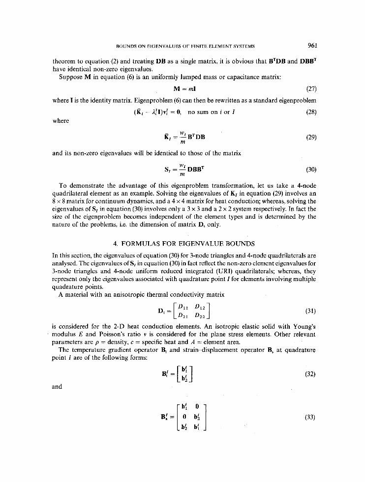
To demonstrate the advantage of this eigenproblem transformation, let us take a %node quadrilateral element as an example. Solving the eigenvalues of KI in equation (29) involves an 8 x 8 matrix for continuum dynamics, and a 4 x 4 matrix for heat conduction; whereas, solving the eigenvalues of SI in equation (30) involves only a 3 x 3 and a 2 x 2 system respectively. In fact the size of the eigenproblem becomes independent of the element types and is determined by the nature of the problems, i.e. the dimension of matrix D, only.

4. FORMULAS FOR EIGENVALUE BOUNDS

In this section, the eigenvalues of equation (30) for 3-node triangles and 4-node quadrilaterals are analysed. The eigenvalues of SI in equation (30) in fact reflect the non-zero element eigenvalues for 3-node triangles and 4-node uniform reduced integrated (URI) quadrilaterals; whereas, they represent only the eigenvalues associated with quadrature point I for elements involving multiple quadrature points.

A material with an anisotropic thermal conductivity matrix

is considered for the 2-D heat conduction elements. An isotropic elastic solid with Young’s modulus E and Poisson’s ratio v is considered for the plane stress elements. Other relevant parameters are p = density, c = specific heat and A = element area.

The temperature gradient operator Bt and strain-displacement operator B, at quadrature point I are of the following forms:

B: = [ ~~] and

B:=[! (33)

962 J. I. LIN

b: and b: stand for the discrete gradient operator at quadrature point Z in the x and y directions respectively. A 2 x 2 matrix a is defined by

aij =2: bf( bj')= (34) We denote a in its principal orientation as P and note that

where li,, Ci2 are the eigenvalues of a and 4, 2 2,. Equation (30) can be expressed in detail as

1 SI =; "[ Dlla l l + D12a12 DllQl2 + D12a22

m D210ll + D22a12 D21a12 + D22422

for heat conduction elements, and

for plane stress elements.

ous to express SI in terms of the eigenvalues of a as Since the material constants in equation (37) are independent of co-ordinates, it is advantage-

0 1 Vlil h2 0

0 0 -(L& + & ) m(1 - v2)

l - v 2

Sf =

The maximal eigenvalue for SI in equation (38) is

(6, + b2 + ,,/(&I - 2 ~ ) ~ + 4V26182) (39)

As for equation (36), it is more efficient solving the quadratic equation computationally in the programs than coding a lengthy formula. However, for the special case of an isotropic thermal conductivity matrix

I WI E 2m(l - v2)

Am& =

Dij = D5ij (40)

A',,, = DCil (41)

the maximal eigenvalue of equation (36) is

To complete these formulas for the maximal eigenvalue at a quadrature point, we need to define m, wI and the gradient operators b:, b: for different cases.

Three-node triangular elements

The superscript/subscript I in equations (34) and (39) can be dropped since no numerical integration is required for this element. The gradient operators bl , b2, m and weight factor w are

BOUNDS ON EIGENVALUES OF FINITE ELEMENT SYSTEMS 963

given by

4 pcA for heat conduction elements m = {+ pA for plane stress elements

w = A where

XIJ = XI - XJ

YIJ = YI - YJ

xJ and yJ are the x and y co-ordinates of node J respectively.

Four-node quadrilateral elements

The gradient operators evaluated at quadrature point I can be expressed as

where J I is the Jacobian evaluated at quadrature point I .

(49) J -1 I - 8 c(x43yZ1 - xZIy43)5I + (X32y41 - x41y32)VI f (x31y42 + X24Y31)l

and rn are given by

and qz represent the reference co-ordinates of quadrature point I. The weight factor wI and

(50) J I for fully integrated (FI) quadrilaterals A for uniform reduced integrated (URI) quadrilaterals

d pcA for heat conduction elements rn = {d pA for plane stress elements

Note that for an FI quadrilateral element

5 2 = 53 = 1113 = 1114 = I/$

51 = 54 = 1111 = 1112 = - I/$

964 J. I. LIN

and its maximal eigenvalue, A,,,, is bounded by

could be determined by equation (36), (39) or (41). For an URI quadrilateral element,

tI = ?I = 0 (54)

and equation (36), (39) or (41) provides the exact maximal element eigenvalue. The plane strain counterpart of equation (39) is

where

- 1 v=- 1 + 2 p

and 1 and p are the Lam6 constants. Because of difficulties in incompressible problems, the selective reduced integration (SRI)

technique is often used for plane strain 4-node quadrilaterals. The maximal element eigenvalue Amax for an SRI quadrilateral can be bounded by

J I and 6: are the Jacobian and b1 evaluated at the quadrature points defined by the reference co-ordinates in equation (52), and 4': and 6: are B1, Ci2 evaluated at the origin of the reference co-ordinates.

Equations (36), (39), (41), (55) and (57) not only provide the system eigenvalue bounds through straight function evaluations, they also use only quantities readily available from the solution procedures. Hence adopting these formulas requires little programming and computational effort.

5. EXAMPLES

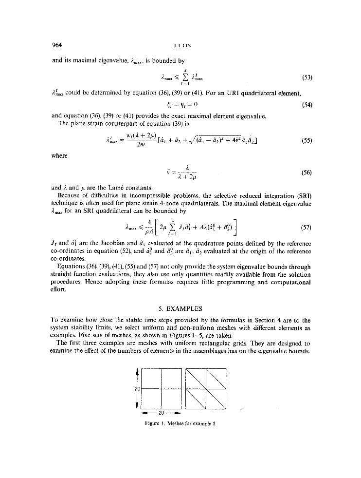
To examine how close the stable time steps provided by the formulas in Section 4 are to the system stability limits, we select uniform and non-uniform meshes with different elements as examples. Five sets of meshes, as shown in Figures 1-5, are taken.

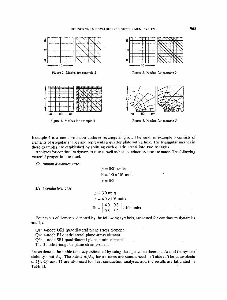
The first three examples are meshes with uniform rectangular grids. They are designed to examine the effect of the numbers of elements in the assemblages has on the eigenvalue bounds.

Figure 1. Meshes for example 1

BOUNDS ON EIGENVALUES OF FINITE'ELEMENT SYSTEMS

t 1 40

- 40-

Figure 2. Meshes for example 2

t 1 80

- 80-

Figure 3. Meshes for example 3

t i 80

-t-- 80-

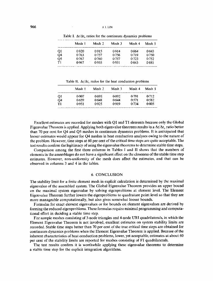
Figure 4. Meshes for example 4

.c- 80-

Figure 5. Meshes for example 5

965

Example 4 is a mesh with non-uniform rectangular grids. The mesh in example 5 consists of elements of irregular shapes and represents a quarter plate with a hole. The triangular meshes in these examples are established by splitting each quadrilateral into two triangles.

Analyses for continuum dynamics case as well as heat conduction case are made. The following material properties are used.

Continuum dynamics case p = 0.01 units E = 1 . 0 ~ lo6 units v = 0.2

Heat conduction case p = 3-0 units c = 4.0 x lo6 units

4*0 O*' x 109 units =I [ 0-8 3.21

Four types of elements, denoted by the following symbols, are tested for continuum dynamics

Q1: 4-node URI quadrilateral plane stress element Q4: 4-node FI quadrilateral plane stress element QS: 4-node SRI quadrilateral plane strain element T1: 3-node triangular plane stress element

studies.

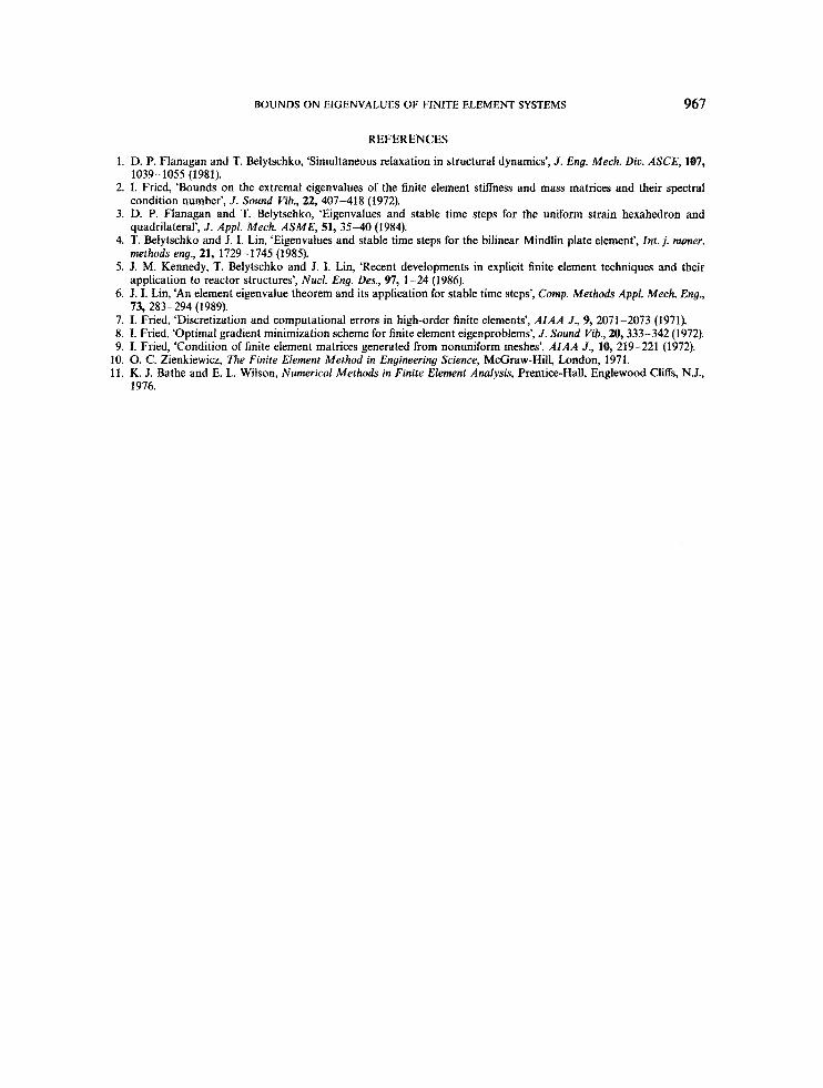
Let us denote the stable time step estimated by using the eigenvalue theorems At and the system stability limit Atc. The ratios At/Atc for all cases are summarized in Table I. The equivalents of Q1, Q4 and TI are also used for heat conduction analyses, and the results are tabulated in Table 11.

966 J. I. LIN

Table I. AtlAt, ratios for the continuum dynamics problems

Mesh 1 Mesh 2 Mesh 3 Mesh 4 Mesh 5

Q1 0.920 0915 0.914 0.864 0.843 0763 0.757 0.756 0.719 0.750 0.767 0.760 0.757 0.723 0.752

T1 0.967 0.955 0.951 0.843 0.881

4 4 Q5

Table 11. AtlAt, ratios for the heat conduction problems

Mesh 1 Mesh 2 Mesh 3 Mesh 4 Mesh 5

0.907 0.895 0.892 0.791 0.712 0.659 0648 0-644 0.571 0.582 0-95 S 0.925 0.919 0734 0.805

Q1 4 4 T1

Excellent estimates are recorded for meshes with Q1 and T1 elements because only the Global Eigenvalue Theorem is applied. Applying both eigenvalue theorems results in a At/Atc ratio better than 70 per cent for 4 4 and Q5 meshes in continuum dynamics problems. It is anticipated that looser estimates would appear for 4 4 meshes in heat conduction analyses owing to the nature of the problem. However, time steps at 60 per cent of the critical time steps are quite acceptable. The test results confirm the legitimacy of using the eigenvalue theorems to determine stable time steps.

Comparison among the first three columns in Tables I and I1 shows that the numbers of elements in the assemblages do not have a significant effect on the closeness of the stable time step estimates. However, non-uniformity of the mesh does affect the estimates, and that can be observed in columns 3 and 4 in the tables.

6. CONCLUSION

The stability limit for a finite element mesh in explicit calculation is determined by the maximal eigenvalue of the assembled system. The Global Eigenvalue Theorem provides an upper bound on the maximal system eigenvalue by solving eigenproblems at element level. The Element Eigenvalue Theorem further lowers the eigenproblems to quadrature point level so that they are more manageable computationally, but also gives somewhat looser bounds.

Formulas for exact element eigenvalues or for bounds on element eigenvalues are derived by forming the reduced eigenproblems. These formulas require minimal programming and computa- tional effort in deciding a stable time step.

For sample meshes consisting of 3-node triangles and 4-node URI quadrilaterals, in which the Element Eigenvalue Theorem is not involved, excellent estimates on system stability limits are recorded. Stable time steps better than 70 per cent of the true critical time steps are obtained for continuum dynamics problems when the Element Eigenvalue Theorem is applied. Because of the inherent characteristics of heat conduction problems, lower, yet acceptable, estimates at about 60 per cent of the stability limits are reported for meshes consisting of FI quadrilaterals.

The test results confirm it is worthwhile applying these eigenvalue theorems to determine a stable time step for the explicit integration algorithms.

BOUNDS ON EIGENVALUES OF FINITE ELEMENT SYSTEMS 967

REFERENCES

1. D. P. Flanagan and T. Belytschko, ‘Simultaneous relaxation in structural dynamics’, J . Eng. Mech. Diu. ASCE, 107,

2. I. Fried, ‘Bounds on the extremal eigenvalues of the finite element stiffness and mass matrices and their spectral

3. D. P. Flanagan and T. Belytschko, ‘Eigenvalues and stable time steps for the uniform strain hexahedron and

4. T. Belytschko and J. 1. Lin, ‘Eigenvalues and stable time steps for the bilinear Mindlin plate element’, Int. j. numer.

5. J. M. Kennedy, T. Belytschko and J. I. Lin, ‘Recent developments in explicit finite element techniques and their

6. J. I. Lin, ‘An element eigenvalue theorem and its application for stable time steps’, Comp. Methods Appl. Mech. Eng.,

7. I. Fried, ‘Discretization and computational errors in high-order finite elements’, AIAA J., 9, 2071-2073 (1971). 8. I. Fried, ‘Optimal gradient minimization scheme for finite element eigenproblems’, J. Sound Vib., 20,333-342 (1972). 9. I. Fried, ‘Condition of finite element matrices generated from nonuniform meshes’, AIAA J., 10,219-221 (1972).

10. 0. C. Zienkiewicz, The Finite Element Method in Engineering Science, McGraw-Hill, London, 1971. 11. K. J. Bathe and E. L. Wilson, Numerical Methods in Finite Element Analysis, Prentice-Hall, Englewood Cliffs, N.J.,

1039-1055 (1981).

condition number’, J. Sound Vib., 22, 407-418 (1972).

quadrilateral’, J. Appl. Mech. ASME, 51, 35-40 (1984).

methods eng., 21, 1729-1745 (1985).

application to reactor structures’, Nucl. Eng. Des., 97, 1-24 (1986).

73, 283-294 (1989).

1976.