HAL Id: hal-00071122https://hal.archives-ouvertes.fr/hal-00071122

Submitted on 23 May 2006

HAL is a multi-disciplinary open accessarchive for the deposit and dissemination of sci-entific research documents, whether they are pub-lished or not. The documents may come fromteaching and research institutions in France orabroad, or from public or private research centers.

L’archive ouverte pluridisciplinaire HAL, estdestinée au dépôt et à la diffusion de documentsscientifiques de niveau recherche, publiés ou non,émanant des établissements d’enseignement et derecherche français ou étrangers, des laboratoirespublics ou privés.

Universal distribution of random matrix eigenvaluesnear the ”birth of a cut” transition.

Bertrand Eynard

To cite this version:Bertrand Eynard. Universal distribution of random matrix eigenvalues near the ”birth of a cut”transition.. Journal of Statistical Mechanics: Theory and Experiment, IOP Publishing, 2006, P07005,pp.P07005. 10.1088/1742-5468/2006/07/P07005. hal-00071122

ccsd

-000

7112

2, v

ersi

on 1

- 2

3 M

ay 2

006

SPT-06/046

Universal distribution of random matrix eigenvalues near the“birth of a cut” transition.

B. Eynard 1

Service de Physique Theorique de Saclay,

F-91191 Gif-sur-Yvette Cedex, France.

Abstract

We study the eigenvalue distribution of a random matrix, at a transition where a

new connected component of the eigenvalue density support appears away from other

connected components. Unlike previously studied critical points, which correspond to

rational singularities ρ(x) ∼ xp/q classified by conformal minimal models and integrable

hierarchies, this transition shows logarithmic and non-analytical behaviours. There is

no critical exponent, instead, the power of N changes in a saw teeth behaviour.

1 Introduction

Random matrix models [20, 13] have been studied in relationship with many areas of

physics and mathematics. The reason of their success for most of their applications is

their “universality” property, i.e. the fact that the eigenvalues statistical distribution

of a large random matrix depends only on the symmetries of the matrix ensemble, and

not on the detailed Boltzmann weight (characterized by a potential). Although this

universality property has been much studied for generic potentials, some universality

should also hold for critical potentials. Different kinds of critical potentials have been

studied, and their universality classes have been found to be in correspondence with

non-linear integrable hierarchies (KdV, MKdV, KP,...) [2, 3, 7, 21, 6, 12], and with

the (p, q) rational minimal models of conformal field theory [8]. They correspond to

rational singularituies of the equilibrium density:

ρ(x) ∼ (x− a)p/q . (1.1)

1E-mail: eynard@spht.saclay.cea.fr

1

In the hermitian 1-matrix model, we have only q = 2 and p arbitrary, thus we get

only half integer singularities (hyperelliptical curves), which are in relationship with

the KdV hierarchies, whereas a 2-matrix model allows to have any rational singularity

(p, q) [8]. The specific heat near such a rational singularity obeys a Gelfand-Dikii-type

equation (Painleve I equation for (p, q) = (3, 2)). A well known case is the edge of

the spectrum where (p, q) = (1, 2), which gives Tracy-Widom law [23], and which is

governed by the Painleve II equation. Another well known case is the merging of two

cuts (Bleher and Its [2, 1]), where (p, q) = (2, 1), which is also governed by a Painleve

II equation as well (indeed, (p, q) and (q, p) are known to be dual to each other [14]).

Here, we shall study a kind of critical point which has been mostly disregarded

(because usual methods don’t apply to it): “the birth of a cut critical point”2.

Such a critical point, is characterized by the fact that when a parameter of the

model (let us call it temperature) is varied, a new connected component appears in the

support of the large N average eigenvalue density. When the temperature T is just

above critical temperature Tc, the number of eigenvalues in the newborn connected

component is small (see fig.2), and thus, many usual large n methods don’t work in

that case.

Our goal is to study the eigenvalues statictics in the vicinity of the critical point,

and find its universality class.

In this purpose, we shall start from the partition function, and treat the eigenvalues

in the other cuts with mean field approximations, and reduce the problem to an effective

partition function for eigenvalues in the newborn cut only, in a method similar to [4].

We find that, unlike rational critical points, the birth of a cut critical point does

not corrsepond to power law behaviors or transcandental differential equations, but it

exhibits logarithmic behaviors, and discontinuous functions.

The matrix model is associated to a family of orthogonal polynomials, whose zeroes

lie inside the connected components of the density [20, 22, 10]. Our goal is also to study

the asymptotic behavior of the orthogonal polynomials in the vicinity of the newborn

cut.

Outline of the article:

- In section 2 we introduce definitions and notations for orthogonal polynomials and

associated quantities.

- In section 3 we recall classical results of random matrix theory: the semiclassical

behaviors of free energy, density, correlation functions, orthogonal polynomials, valid

away from critical points.

2Name suggested by P. Bleher who initiated this work.

2

effV (x)

e~ eba x

Figure 1: The “birth of a cut” critical potential is such that one of the potential wellsof the effective potential is just at the Fermi level. At a νth order critical point, theeffective potential behaves like Veff(e) + 1

2ν!V

(2ν)eff (e) (x− e)2ν + . . ..

- In section 4 we study the analytical continuation of the previous semiclassical ap-

proximations, near the “birth of a cut” critical point (divergencies at critical point).

- In section 5 we compute the partition function with mean field theory for eigenvalues

not in the newborn cut, and derive an effective partition function for the newborncut

eigenvalues.

- In section 6 we use the results of section 5 to deduce the asymptotic behaviors of

correlation functions and orthogonal polynomials in the vicinity of the critical point.

- Section 7 is the conclusion.

- In appendix, we recall Stirling’s formula and its consequences, and we recall some

elliptical function basics.

2 Setting

Given an integer n (we will later consider the limit n → ∞), a real polynomial V (x)

called the potential:

V (x) := g0 +

d+1∑

k=1

gk

kxk , deg V = d+ 1 (2.2)

3

ρ( )x

a b e x

Figure 2: The “birth of a cut” density of eigenvalues is such that one of the connectedcomponents of the support contains a very small number of eigenvalues (≪ n).

of even degree and positive leading coefficient (gd+1 > 0), and a temperature T > 0,

we define the partition function:

Zn(T, V ) :=1

n!

∫

Rn

dx1 . . .dxn (∆(xi))2

n∏

i=1

e−nT

V (xi) (2.3)

(where ∆(xi) =∏

i<j(xj − xi) is the Vandermonde determinant) and the free energy

Fn(T, V ):

e−n2

T2 Fn(T,V ) :=Zn(T, V )

Hn(2.4)

where Hn is a combinatorial normalization:

Hn := (2π)n/2 n−n2/2 e3/4n2n−1∏

k=0

k! = 2n/2 πn2/2 n−n2/2 e3/4n2

n!Un(2.5)

and Un is the volume of the group U(n)/U(1)n.

Then we define the resolvent:

Wn(x, T, V ) :=T

n!Zn(T, V )

∫

dx1 . . .dxn1

x− x1∆2(xi)

n∏

i=1

e−nT

V (xi) (2.6)

and its first moment:

Tn(T, V ) :=T

n!Zn(T, V )

∫

dx1 . . .dxn x1 ∆2(xi)

n∏

i=1

e−nT

V (xi)

=1

2iπ

∮

xWn(x, T, V )dx =∂Fn(T, V )

∂g1(2.7)

Notice that more generally for k > 0:

k∂Fn(T, V )

∂gk

=1

2iπ

∮

xkWn(x, T, V )dx (2.8)

4

Then, given a temperature Tc and an integer N , we define:

hn :=Zn+1(Tc

n+1N, V )

Zn(TcnN, V )

, (2.9)

and

γn :=

√

hn

hn−1

=

√

Zn+1(Tcn+1N, V )Zn−1(Tc

n−1N, V )

Z2n(Tc

nN, V )

, (2.10)

and

βn :=N

Tc

(

Tn+1(Tcn+ 1

N, V ) − Tn(Tc

n

N, V )

)

= −Tc

N

∂ lnhn

∂g1

. (2.11)

Notice that Zn(T, V ), hn and γn are strictly positive for all n, in particular they don’t

vanish.

We also introduce the functions [22, 20, 10]:

πn(ξ) =Zn(Tc

nN, V (x) − Tc

Nln (ξ − x))

Zn(TcnN, V )

, , ψn(ξ) =πn(ξ)√hn

e−N2T

V (ξ) (2.12)

which form an orthogonal family of monic polynomials (deg πn = n):

∫

πn(ξ)πm(ξ)e−NTc

V (ξ)dξ = hnδnm , (2.13)

and which satisfy the 3-terms recursion relation:

ξ πn(ξ) = πn+1(ξ) + βn πn(ξ) + γ2n πn−1(ξ) . (2.14)

And we introduce the functions:

πn(ξ) =Zn+1(Tc

n+1N, V (x) + Tc

Nln (ξ − x))

Zn(TcnN, V )

, , φn(ξ) =πn(ξ)√hn

eN2T

V (ξ) (2.15)

which are the Hilbert transforms of the πn(x):

πn(x) =

∫

dx′

x− x′πn(x′)e−V (x′) , (2.16)

and which satisfy the same 3-terms recursion relation, with an initial term:

ξ πn(ξ) = πn+1(ξ) + βn πn(ξ) + γ2n πn−1(ξ) + δn,0h0 . (2.17)

We also define the kernel:

Kn(ξ, y) :=n−1∑

j=0

1

hjπj(ξ)πj(y) e−

N2Tc

(V (ξ)+V (y)) , (2.18)

5

and it is well known that all correlation functions can be expressed in term of that

kernel (Dyson’s theorem [15, 20]):

ρn(x) =1

nKn(x, x)

ρn(x, y) =1

n2(Kn(x, x)Kn(y, y)−Kn(x, y)Kn(y, x))

. . . (2.19)

and that we have the Christoffel-Darboux theorem:

Kn(x, y) =1

hn−1

πn(x)πn−1(y) − πn−1(x)πn(y)

x− ye−

N2Tc

(V (x)+V (y)) . (2.20)

Our goal is to study γn, βn, πn, πn, in the vicinity of N → ∞, and |n − N | ≪ N ,

and with Tc chosen such that we are at a special critical point described below.

For the moment, let us study the large N -limits away from the critical point.

3 Classical limits

It is well known that in the semiclassical limit N → ∞, and |n−N | ≪ N , if T 6= Tc,

the free energy has a large n limit [11, 16, 4, 19, 13]:

Fn(T, V ) −→ F (T, V ) +O(1/n2) (3.21)

and so has the resolvent Wn(x, T, V ):

Wn(x, T, V ) −→W (x, T, V ) +O(1/n) (3.22)

3.1 The large n resolvent

It is well known that, if the potential is such that V ′(x) is a rational fraction, with its

poles outside the cuts (that assumption will become clear below), the large n resolvent

W (x, T, V ) can be written as the solution of an hyperelliptical equation [13, 5]:

W (x, T, V ) =1

2

(

V ′(x) −M(x, T, V )√

σ(x, T, V ))

(3.23)

where σ is a monic even degree (2s ≥ 2) polynomial with distinct simple zeroes only:

σ(x) =s∏

i=1

(x− ai)(x− bi) , . . . < ai < bi < ai+1 < . . . (3.24)

whose zeroes are called the endpoints, and⋃s

i=1[ai, bi] is called the support, and M is

a rational function with the same poles as V ′. If one assumes that s and σ are known,

6

M(x, T, V ) is determined by the condition that W (x, T, V ) is finite (in the physical

sheet) when x→ ∞ and when x approaches the poles of V ′(x).

The large n limit of the density of eigenvalues is then:

ρ(x, T, V ) =1

2πTM(x, T, V )

√

−σ(x, T, V ) , x ∈s⋃

i=1

[ai, bi] (3.25)

We also define the effective potential:

Veff(x, T, V ) := V (x) − 2T ln x− 2

∫ x

∞

(

W (x, T, V ) − T

x

)

dx (3.26)

Notice that its derivative is V ′(x) − 2W (x, T, V ) = M(x, T, V )√

σ(x, T, V ).

So far, we have not explained how to determine s and the polynomial σ. If one

assumes that s is known, σ(x, T, V ) is determined by the conditions:

W (x, T, V ) ∼x→∞

T

x+O(1/x2)

if s > 1, ∀i = 1, . . . , s− 1, Veff(bi) = Veff(ai+1)(3.27)

The large n free energy is then given by:

F (T, V ) =1

4iπ

∮

W (x, T, V )V (x)dx+1

2TVeff(bs) (3.28)

where the integration contour is a counter clockwise circle around ∞.

The number of endpoints s = s(T, V ), (we have 1 ≤ s ≤ d) is determined by the

condition that the free energy is minimum (one can prove that s(T, V ) ≤ (d + 1)/2)

[9].

3.2 Derivatives with respect to T

Let us introduce:

Ω(x, T, V ) :=∂W (x, T, V )

∂T=QΩ(x, T, V )√

σ(x, T, V )(3.29)

where QΩ(x, T, V ) is a monic polynomial of degree s−1, determined by the conditions:

if s > 1, ∀i = 1, . . . , s− 1,

∫ ai+1

bi

QΩ(x, T, V )√

σ(x, T, V )dx = 0 (3.30)

In algebraic geometry, Ω is called ”normalized abelian differential of the third kind”

[18, 17].

We introduce the multivalued function Λ(x, T, V ):

Λ(x, T, V ) := exp

(∫ x

bs

Ω(x′, T, V ) dx′)

(3.31)

7

and

γ(T, V ) := limx→∞

x

Λ(x, T, V )(3.32)

Then we have the following derivatives:

∂F

∂T= Veff(bs) (3.33)

∂2F

∂T 2= −2 ln γ (3.34)

∂Veff(x)

∂T= −2 ln (γΛ(x)) (3.35)

∂T∂T

=1

2iπ

∮

xΩ(x) dx (3.36)

Notice that:

Veff(bs) =1

2iπ

∮

ΩV − 2T ln γ (3.37)

3.3 Poles of the potential

Assume that V ′(x) has a simple pole at x = ξ, with residue r (it may have other poles

too), then we define the function:

H(x, ξ, T, V ) :=∂W (x, T, V )

∂r=

1

2√

σ(x)

(

√

σ(x) −√

σ(ξ)

x− ξ−QH(x, ξ)

)

(3.38)

where QH(x, ξ) is a monic polynomial in x, of degree s−1, determined by the conditions:

if s > 1, ∀i = 1, . . . , s− 1,

∫ ai+1

bi

QH(x, ξ, T, V ) +

√σ(ξ)

x−ξ√

σ(x, T, V )dx = 0 (3.39)

We also define its (multivalued) primitive:

lnE(x, ξ) :=

∫ x

∞

H(x′, ξ) dx′ (3.40)

Notice that it is finite near the endpoints and near x = ξ. In algebraic geometry,

(x− ξ)/E(x, ξ) is related to the ”prime form” [18, 17].

Then we have:∂Veff(x)

∂r= ln (x− ξ) − 2 lnE(x, ξ) (3.41)

∂T∂T

=1

2iπ

∮

xH(x, ξ) dx (3.42)

8

∂F

∂r=

1

2(V (x) − Veff(x))|x=ξ (3.43)

∂2F

∂r∂T= ln (γΛ(ξ)) = ln (ξ − bs) − 2 lnE(bs, ξ) (3.44)

If V ′(x) has simple poles at x = ξ1 with residue r1 and at x = ξ2 with residue r2,

we have:∂2F

∂r1∂r2= lnE(ξ1, ξ2) (3.45)

and thus it is clear that lnE has some symmetry properties: lnE(x, y) = lnE(y, x).

3.4 1-cut case

If W (x, T, V ) has one cut [a(T, V ), b(T, V )] with a < b, we use the Joukowski’s param-

eterization:

x =b+ a

2+b− a

2coshφ (3.46)

i.e.√

σ(x) =b− a

2sinhφ (3.47)

We have:

Ω(x) =1

√

(x− a)(x− b)=∂φ

∂x, Λ(x) = eφ(x) , γ =

b− a

4(3.48)

H(x, ξ) =∂φ(x)

∂x

1

eφ(x)+φ(ξ) − 1, E(x, ξ) = 1 − e−(φ(x)+φ(ξ)) =

x− ξ

Λ(x) − Λ(ξ)(3.49)

∂T∂T

=a + b

2,

∂T∂r

=γ

Λ(ξ)(3.50)

Then, it is well known [] that we have the large n,N asymptotics (in the regime

n/N =finite):

γn ∼ b(TcnN

) − a(TcnN

)

4, βn ∼ b(Tc

nN

) + a(TcnN

)

2(3.51)

3.5 2-cut case

If W (x, T, V ) has two cuts [a(T, V ), b(T, V )] ∪ [c(T, V ), d(T, V )] with a < b < c < d,

Let m be their biratio:

m =(b− a)(d− c)

(c− a)(d− b)(3.52)

9

We parameterize:

x(u) = d− d− a

1 + b−ad−b

sn2(u,m)(3.53)

where sn is tha elliptical sine function (see appendix I, or for instance [24]), i.e., by

definition:

u(x) := − i

2

√

(d− b)(c− a)

∫ x

a

dy√

σ(y)=

∫

√

d−bb−a

x−ad−x

0

dy√

(1 − y2)(1 −my2)(3.54)

We have:

u(a) = 0, u(b) = K(m),

u(c) = K(m) + iK ′(m), u(d) = iK ′(m). (3.55)

We have:

√

σ(x) = −i(d − a)(b− a)

√

c− a

d− b

sn(u,m) cn(u,m) dn(u,m)

(1 + b−ad−b

sn2(u,m))2. (3.56)

Let us define u∞ such that:

u∞ := i

∫

√

d−bb−a

0

dy√

(1 + y2)(1 +my2), (3.57)

i.e.

sn(u∞, m) = i

√

d− b

b− a, , cn(u∞, m) =

√

d− a

b− a, , dn(u∞, m) =

√

(d− a)

(c− a). (3.58)

Then we define x0:

x0 = d+ i√

(c− a)(d− b)

(

E(u∞, m) −(

1 − E ′(m)

K ′(m)

)

u∞

)

. (3.59)

It satisfies:∫ c

b

x− x0√

(x− a)(x− b)(x− c)(x− d)dx = 0, (3.60)

thus we have:

Ω(x) =x− x0

√

(x− a)(x− b)(x− c)(x− d)(3.61)

Λ(x) = eπu(x)u∞

KK′θ1((u(x) + u∞)/2K)

θ1((u(x) − u∞)/2K)(3.62)

γ =i

4K

√

(d− b)(c− a) e−πu2∞

KK′θ′1(0, τ)

θ1(u∞/K, τ)(3.63)

10

E(x, ξ) =θ1(u(x) + u(ξ)) θ1(2u∞)

θ1(u∞ + u(ξ)) θ1(u∞ + u(x))(3.64)

∂T∂T

=a + b+ c + d

2− x0 (3.65)

we have the asymptotics [11, 4]:

d(TcnN

) − a(TcnN

) − c(TcnN

) + b(TcnN

)

4≤ γn ≤ d(Tc

nN

) − a(TcnN

) + c(TcnN

) − b(TcnN

)

4(3.66)

d(TcnN

) + a(TcnN

) − c(TcnN

) + b(TcnN

)

2≤ βn ≤ d(Tc

nN

) + a(TcnN

) + c(TcnN

) − b(TcnN

)

2(3.67)

Therefore, we shall now study W (x, T, V ) in different regimes.

4 The Birth of a cut critical point

Let us choose the potential V and the temperature Tc such that:

• for T < Tc we are in a one-cut case,

W (x, T ) =1

2

(

V ′(x) −M−(x, T )√

(x− a)(x− b))

(4.68)

with a(T ) < b(T ) and

M−(x, Tc) = (x− e)2ν−1Q(x) , (4.69)

where ν ≥ 1 is an integer, and Q(x) is a real polynomial whose properties are

described bellow.

• for T > Tc we are in a two-cuts case,

W (x, T ) =1

2

(

V ′(x) −M+(x, T )√

(x− a)(x− b)(x− c)(x− d))

(4.70)

with a(T ) < b(T ) < c(T ) < d(T ) and

c(Tc) = d(Tc) = e , M+(x, Tc) = (x− e)2ν−2 Q(x) , (4.71)

• at T = Tc one cut has vanishing size c(Tc) = d(Tc). With no loss of generality,

we can assume that:

a(Tc) = −2 , b(Tc) = 2, (4.72)

and we write:

e(Tc) = 2 coshφe = c(Tc) = d(Tc) (4.73)

11

The polynomial Q(x) must have the following properties:

• degQ = d− 2ν with d odd and d > 2ν,

• The leading coefficient of Q is positive,

• Q has an odd number of zeroes in ]2, e[,

• Q(x) < 0 in [−2, 2],

• Q(e) > 0,

•∀x < −2,

∫ −2

x

Q(x)(x− e)2ν−1√x2 − 4 dx > 0 (4.74)

•∀x > 2, x 6= e,

∫ x

2

Q(x)(x− e)2ν−1√x2 − 4 dx > 0 (4.75)

•∫ e

2

Q(x)(x− e)2ν−1√x2 − 4 dx = 0 (4.76)

•V ′(x) = Pol

x→∞

(

(x− e)2ν−1Q(x)√x2 − 4

)

(4.77)

•Tc =

1

2Res∞

(x− e)2ν−1Q(x)√x2 − 4 dx (4.78)

Remark: notice that for all ν ≥ 1, it is possible to find a potential V (x) and a tem-

perature Tc with such properties. Indeed, choose e and Q(x) with the above properties

and determine V ′(x) and Tc by 4.77 and 4.78. Notice also that it is always possible to

find a polynomial Q(x) which satisfies the above mentioned conditions, indeed consider

any real e > 2, and any real polynomial Q(x), of even degree d− 2ν − 1, with positive

leading coefficient, and with no real zero, then set:

e =

∫ e

2x Q(x) (x− e)2ν−1

√x2 − 4 dx

∫ e

2Q(x) (x− e)2ν−1

√x2 − 4 dx

(4.79)

clearly, e ∈]2, e[, and then set:

Q(x) = (x− e)Q(x) (4.80)

In particular, one may choose d = 2ν + 1 and Q = 1.

12

4.1 Example ν = 1

Let e > 2 be fixed. We write e = 2 coshφe.

We consider the following quartic potential:

V ′(x) =(

x3 − (e+ e)x2 + (ee− 2)x+ 2(e+ e))

, Tc = 1 + ee (4.81)

where e is given by∫ e

2(x− e)(x− e)

√x2 − 4 = 0, i.e. :

e = 2φe coshφe − 1

3sinh φe(2 + cosh2 φe)

13sinhφe cosh φe(5 − 2 cosh2 φe) − φe

(4.82)

4.2 At the critical point T = Tc:

At T = Tc, both formula 4.68 and 4.70 reduce to:

W (x, Tc) =1

2

(

V ′(x) − (x− e)2ν−1Q(x)√x2 − 4

)

(4.83)

which would correspond to an average large N eigenvalue density in [−2, 2]:

ρ(x) =1

2πTc

(x− e)2ν−1Q(x)√

4 − x2 (4.84)

and one would have:

γN ∼ 1 , βN ∼ 0 (4.85)

However, this is wrong, because the semiclassical asymptotics 3.22 are valid only if

T 6= Tc, they break down at T = Tc. It is the purpose of section 5, to determine the

asymptotic behavior of γn and βn near n = N and T = Tc. For the moment, let us

consider the limits of 4.68 and 4.70 near Tc.

4.3 Variations near the critical point, T < Tc (one-cut)

Let us consider the limit of 4.68 near Tc. Write T = Tc + t, and t < 0, and:

W (x, T ) =1

2

(

V ′(x) −M−(x, T )√

(x− a)(x− b))

(4.86)

At T = Tc we have

a(Tc) = −2 , b(Tc) = 2 , M−(x, Tc) = (x− e)2ν−1Q(x) , (4.87)

Then, make use of formula 3.29 and 3.48, i.e.

− 1

2

∂M−(x, T )

∂T+

1

4M−(x, T )

∂a∂T

(x− a)+

1

4M−(x, T )

∂b∂T

(x− b)=

1

(x− a)(x− b)(4.88)

13

matching the pole at x = a gives:

∂a

∂T=

4

(a− b)M−(a, T )∼ − 1

(a− e)2ν−1Q(a)(4.89)

which is finite at T = Tc, thus, we find that to first order in t:

a ∼ −2 +t

(2 + e)2ν−1Q(−2), b ∼ 2 − t

(e− 2)2ν−1Q(2)(4.90)

(notice that Q(−2) < 0 and Q(2) < 0). Relation 3.48 implies:

γ ∼ 1 +O(t) (4.91)

Then, 4.88 reduces to:

1

2

∂M−(x, T )

∂T=

M−(x, T ) −M−(a, T )

M−(a, T )(a− b)(x− a)+

M−(x, T ) −M−(b, T )

M−(b, T )(b− a)(x− b)(4.92)

which is finite at T = Tc, thus one gets the asymptotics of M−:

2∂M−(x, T )

∂T= −(x− e)2ν−1(Q(x) −Q(a)) + ((x− e)2ν−1 − (a− e)2ν−1)Q(a)

(a− e)2ν−1 Q(a) (x− a)

+(x− e)2ν−1(Q(x) −Q(b)) + ((x− e)2ν−1 − (b− e)2ν−1)Q(b)

(b− e)2ν−1Q(b) (x− b)

= − (x− e)2ν−1

(a− e)2ν−1Q(a)

Q(x) −Q(a)

x− a− (x− e)2ν−1 − (a− e)2ν−1

(x− a) (a− e)2ν−1

+(x− e)2ν−1

(b− e)2ν−1Q(b)

Q(x) −Q(b)

x− b+

(x− e)2ν−1 − (b− e)2ν−1

(x− b) (b− e)2ν−1

(4.93)

in particular in the vicinity of x = e one has:

M−(x, T ) ∼ (x− e)2ν−1Q(x)

+t

2

[

2ν−2∑

k=0

(x− e)k((2 − e)−k−1 − (−2 − e)−k−1) +O(x− e)2ν−1

]

(4.94)

Note that the zeroes of M−(x, T ) in the vicinity of e, are the 2ν − 1th roots of unity:

M−(x, Tc + t) = 0 ↔ x = e+

(

2t

Q(e)(e2 − 4)

)1/2ν−1

+O(t2/2ν−1) (4.95)

Using 3.51, we get:

γn ∼ 1 − t

4

(

1

(e− 2)2ν−1Q(2)+

1

(e+ 2)2ν−1Q(−2)

)

βn ∼ − t

2

(

1

(e− 2)2ν−1Q(2)− 1

(e+ 2)2ν−1Q(−2)

)

where n = N(1 + t/Tc) (4.96)

14

4.4 Variations near the critical point, T > Tc (two cuts)

Let us consider the limit of 4.70 near Tc. Write T = Tc + t, and t > 0,and

W (x, T ) =1

2

(

V ′(x) −M+(x, T )√

(x− a)(x− b)(x− c)(x− d))

(4.97)

At T = Tc we have

a(Tc) = −2 , b(Tc) = 2

c(Tc) = d(Tc) = e = 2 coshφe , M+(x, Tc) = (x− e)2ν−2Q(x) , (4.98)

and at T > Tc, a + 2, b − 2, c− e, d − e, and M+(x) − (x − e)2ν−2Q(x) are small. In

particular, we write:

M+(x, T ) = H(x, T )Q(x, T ) (4.99)

where H(x, T ) is a monic polynomial of degree 2ν − 2 which contains all the roots of

M+ close to e, and Q(x, T ) is the remaining part. In other words, H(x, T )− (x−e)2ν−2

is small and Q(x, T ) −Q(x) is small in the small t limit.

We use the notations of section 3.5. The biratio 3.52 is thus:

m =(b− a)(d− c)

(c− a)(d− b)∼ 4

e2 − 4(d− c) ∼ d− c

sinh2 φe

(4.100)

we see that we have to consider the limit m→ 0. In that limit 3.57 becomes

u∞ = i

∫

√

d−bb−a

0

dy√

(1 + y2)(1 +my2)∼ i

∫

√e−24

0

dy√

1 + y2= i

φe

2(4.101)

E(u∞) − u∞ = im

∫

√

d−bb−a

0

y2 dy√

(1 + y2)(1 +my2)

∼ im

∫

√e−24

0

y2 dy√

(1 + y2)= im

sinh φe − φe

4

(4.102)

And, as can be found in any handbook of classical functions [], we have the small m

behavior:E ′(m)

K ′(m)∼ − 2

lnm(4.103)

Since for small m one has∣

∣

1ln m

∣

∣≫ m, 3.59 becomes:

δx0 := x0 − d ∼ 2φe sinh φe

lnm(4.104)

15

Notice that:

x0 − c = x0 − d+ d− c ∼ x0 − d+m sinh2 φe ∼ x0 − d ∼ δx0 (4.105)

From 3.29 and 3.61 we have:

− 1

2

∂M+(x, T )

∂T− 1

4

M+(x, T )

σ(x, T )

∂σ(x, T )

∂T=

x− x0

σ(x, T )(4.106)

Matching the pole at x = c gives:

∂c

∂t=

−4(d− c+ δx0)

(c− a)(c− b)(c− d)M+(c, Tc + t)∼ −4δx0

(e2 − 4)Q(e)

1

(c− d)H(c)(4.107)

and matching the pole at x = d gives:

∂d

∂t=

−4δx0

(d− a)(d− b)(d− c)M+(d)∼ − 4δx0

(e2 − 4)Q(e)

1

(d− c)H(d)(4.108)

and matching the poles close to e gives:

∂H(x)

∂t∼ − 2δx0

(e2 − 4)Q(e)

1

d− c

(

H(x) −H(d)

(x− d)H(d)− H(x) −H(c)

(x− c)H(c)

)

(4.109)

The following guess solves the 3 equations 4.107, 4.108, 4.109 to small t leading

order:

c ∼ e− 2ζ

(

− t

ln t

)12ν

, d ∼ e+ 2ζ

(

− t

ln t

)12ν

(4.110)

H(x) ∼(

− t

ln t

)−1+ 1ν

G

(

(x− e)

(

− t

ln t

)−12ν

)

(4.111)

where ζ is a positive real number, and G is a degree 2ν − 2 even monic polynomial,

which will be determined below.

For later convenience, we also define the following positive constant:

C :=4ν2φe

sinh φeQ(e)> 0 (4.112)

Using ansatz 4.110 and 4.104, we have in that limit:

δx0 ∼4νφe sinh φe

ln t(4.113)

Then, inserting 4.110 and 4.111 into 4.107 and 4.108, we get:

4ζ2 =C

G(−2ζ)=

C

G(2ζ)(4.114)

16

Then, setting x = e+ξ(

− tln t

)12ν , and inserting 4.111 into 4.109 we get the following

equation for G:

(2ν − 2)G(ξ) − ξ G′(ξ) =C

4ζ

(

G(ξ) −G(2ζ)

(ξ − 2ζ)G(2ζ)− G(ξ) −G(−2ζ)

(ξ + 2ζ)G(−2ζ)

)

(4.115)

which using 4.114 becomes:

(2ν − 2)G(ξ) − ξ G′(ξ) =4ζ2

ξ2 − 4ζ2(G(ξ) −G(2ζ)) (4.116)

the solution of which is:

G(ξ) =ν−1∑

k=0

2k!

k!k!ζ2k ξ2(ν−1−k) = Pol

ξ2ν−1

√

ξ2 − 4ζ2(4.117)

or:

G(2ζ coshψ) = ζ2ν−2ν−1∑

j=0

(

2ν − 1ν + j

)

sinh (2j + 1)ψ

sinhψ(4.118)

In particular,G(2ζ)

ζ2ν−2=

1

2

2ν!

ν − 1!ν!=

C

4ζ2ν(4.119)

i.e. the parameter ζ is determined by:

ζ =

(

C

2

ν! ν − 1!

2ν!

)12ν

=

(

2ν2φe

sinhφeQ(e)

ν! ν − 1!

2ν!

)12ν

(4.120)

In that scaling regime, we have:

m ∼ 4ζ

sinh2 φe

(

− t

ln t

)12ν

(4.121)

i.e. this corresponds to a torus of modulus

τ = iK ′

K∼ −i

πlnm ∼ −i

2νπln t (4.122)

and, using 3.63:

γ =i

4K

√

(d− b)(c− a) e−πu2∞

KK′θ′1(0, τ)

θ1(u∞/K, τ)

∼ e−πu2∞

KK′

∼ 1 − φ2e

lnm

∼ 1 − 2νφ2e

ln t(4.123)

17

we also find that the filling fraction in the [c, d] cut is of order:

ǫ =1

2πTc

∫ d

c

ρ(x) dx

∼ − t

ln t

sinhφeQ(e)

πTc

∫ 2ζ

−2ζ

G(ξ)√

4ζ2 − ξ2 dξ

∼ −i tln t

sinh φeQ(e)

πTc

∫ 2ζ

−2ζ

ξ2ν−1 G(ξ)√

4ζ2 − ξ2

ξ2ν−1dξ

(4.124)

then, integrating by parts and using 4.116, we find:

ǫ ∼ it

Tc ln t

sinhφeQ(e)

2νπ

∫ 2ζ

−2ζ

ξ2ν 4ζ2 ξ−2ν

√

ξ2 − 4ζ2G(2ζ) dξ

∼ it

Tc ln t

sinhφeQ(e)

2νπ4ζ2 G(2ζ)

∫ 2ζ

−2ζ

dξ√

ξ2 − 4ζ2

∼ − t

Tc ln t

sinhφeQ(e)

2νC

(4.125)

i.e.

ǫ(Tc + t) ∼ − t

Tc ln t2νφe (4.126)

This means that for n = N(1 + t/Tc), the average number of eigenvalues located near

e is:

k ∼ n−N

lnN2νφe (4.127)

i.e. the eigenvalues start to explore the potential well near e when n−N ∼ lnN .

According to 3.66 and 3.67, the coefficients γn and βn vary between:

1 + ζ

(−tln t

)12ν

≤ γn ≤ coshφe (4.128)

2ζ

(−tln t

)12ν

≤ βn ≤ e− 2 (4.129)

where n = N(1 + t/Tc)

The transition takes place on a scale of order p ∼ lnN .

4.5 Order of the transition

From 3.34 and 4.91 we have below Tc, i.e. for t < 0:

∂2F

∂t2(Tc + t) = −2 ln γ ∼ t

2

(

1

(e− 2)2ν−1Q(2)+

1

(e+ 2)2ν−1Q(−2)

)

(4.130)

18

and above Tc, i.e. for t > 0, we have from 4.123:

∂2F

∂t2(Tc + t) = −2 ln γ ∼ 4νφ2

e

ln t(4.131)

The second derivative of the free energy is continuous, but the third derivative is not.

therefore we have a third order transition, with logarithmic divergency, cf fig.3.

F∂2

∂2

t

t0

Figure 3: Behavior of the second derivative of the classical free energy with respect tot near the transition.

5 Mean field asymptotics for the partition function

We compute the partition function for a potential:

Vr0(x) = V (x) + r0 ln (x0 − x) (5.132)

where r0 is assumed of order 1/N :

r0 = −aTc

N(5.133)

5.1 Mean Field theory

We use the same idea as in [4]. We split the 2-cuts integral into 1-cut integrals. Let us

say that there are k eigenvalues in the new cut (near e), and n− k in the old cut [a, b]:

n!Zn(n

NTc, Vr0)

19

∼n∑

k=0

(

nk

)∫

xi>e

dx1 . . . dxk ∆2(xi)

k∏

i=1

(x0 − xi)a e−

NTc

V (xi)

(n− k)!Zn−k(Tcn− k

N,Vr0,rj

)

(5.134)

where

Vrj(x) =

k∑

j=0

rj ln (xj − x) , r0 = −aTc

N, r1 = . . . = rk = −2Tc

N

(5.135)

and Zn−k(Tcn−kN,Vrj

)is a one-cut integral:

Zn−k(Tcn− k

N,Vrj

) :=1

n− k!

∫

<e

dxk+1 . . .dxn ∆2(xi)n∏

i=k+1

e−NTc

Vrj(xi)

= Hn−k e−N2

T2c

Fn−k(Tcn−kN

,Vrj )(5.136)

That gives:

Zn(n

NTc, Vr0)

∼n∑

k=0

Hn−k

k!

∫

xi>e

dx1 . . .dxk ∆2(xi)

k∏

i=1

(x0 − xi)a e−

NTc

V (xi) e−N2

T2c

F n−k(Tcn−kN

,Vrj )

(5.137)

In other words, we integrate out n − k eigenvalues, and consider the integral over k

eigenvalues only. The k remaining eigenvalues are submitted to the potential V , as well

as their mutual Coulomb repulsion, and the mean field of the exterior n−k eigenvalues.

Since F n(T,Vrj) corresponds to a one-cut distribution, it can be evaluated with

standard semiclassical technique (see section 3), and in particular, it has a large n

expansion:

F n(T,Vrj) ∼ F (T,Vrj

) +T

nF

(1/2)(T,Vrj

) +T 2

n2F

(1)(T,Vrj

) +O(1

n3) (5.138)

and each term of the expansion is analytical in Vrj.

We want to evaluate F (T,Vrj) in a regime where T − Tc is ”small” (we make that

more precise below) and r0 and the rj’s are of order O(1/N).

we first do a Taylor expansion in T − Tc and the rj’s:

F (T,Vrj) ∼ F (Tc, V ) +

k∑

i=0

ri∂F

∂ri+

1

2

∑

i,j

rirj∂2F

∂ri∂rj+ o(

k2

N2)

+∑

j

(T − Tc)rj∂2F

∂T∂rj

20

+(T − Tc)∂F

∂T+

1

2(T − Tc)

2∂2F

∂T 2+ o(

1

N2) (5.139)

where all derivatives are computed at T = Tc and ri = 0 (see section 3.2 and 3.3).

That expansion is valid only if k ≪ N .

Thus we have:

1

HnZn(

n

NTc, Vr0) ∼ e

−N2

T2c

F (Tc,V )e−F

(1)(Tc,V )ea N

TcF r0e−

a2

2F r0,r0

n∑

k=0

1

k!

Hn−k

Hn

e−NTc

(n−N−k)F T ea(n−N−k)F T,r0e−(n−N−k)2

2F T,T

∫

xi>e

dx1 . . .dxk ∆2(xi)∏

i

(x0 − xi)a e−

NTc

V (xi)

k∏

j=1

e2 NTc

F rj e2(n−N−k)F T,rj e−2aF r0,rj

∏

j,l≥1

e−2F rl,rj

(5.140)

Notice that:Hn−k

Hn∼ (2π)−k(1 − k

n)−1/12(1 +O(1/n)) (5.141)

5.2 Computation of the derivatives

Now, use formula given in section 3.2 and 3.3 in the one-cut case, and get (derivatives

taken at T = Tc and ri = 0, and take into account that Veff(b) = Veff(e)):

∂

∂riF = −1

2(Veff(xi) − V (xi)) ,

∂

∂TF = Veff(e) (5.142)

∂2

∂ri∂rj

F = lnxi − xj

Λ(xi) − Λ(xj),

∂2

∂r2i

F = − ln Λ′(xi) (5.143)

∂2

∂T∂riF = ln Λ(xi) ,

∂2

∂T 2F = 0 (5.144)

Moreover:

∂T (T, V )

∂T=a+ b

2= 0 ,

∂T (T, V )

∂rj=

1

Λ(xj)(5.145)

The effective potential behaves in the vicinity of e as:

Veff(x) ∼x→e

Veff(e) +V

(2ν)eff (e)

2ν!(x− e)2ν (5.146)

V(2ν)eff (e)

2ν!=

2 sinhφeQ(e)

2ν(5.147)

21

In the limit where the xi’s are close to e, we have:

xi − xj

Λ(xi) − Λ(xj)∼

xi,xj→e

1

Λ′(xi)∼ 2 sinhφe e−φe (5.148)

and

Λ(xi) ∼xi→e

eφe (5.149)

5.3 Result

write n = N + p:

ZN+p(N + p

NTc, Vr0) ∼ e

−N2

T2c

F (Tc,V )e−F

(1)(Tc,V )

(

eφe

2 sinhφe

)

a2

2

e−aN2Tc

(Veff (x0)−V (x0))

N+p∑

k=0

HN+p−k

k!e−

NTc

(p−k)Veff (e) ea(p−k)φe

∫

xi>e

dx1 . . .dxk ∆2(xi)k∏

i=1

(x0 − xi)a e−

NTc

V (xi)

k∏

i=1

e−NTc

(Veff (xi)−V (xi)) e2k(p−k)φe

(

eφe

2 sinhφe

)2ak+2k2

∼ HN e−N2

T2c

F (Tc,V )e−F

(1)(Tc,V ) e−

aN2Tc

(Veff (x0)−V (x0)) e−p NTc

Veff (e)

N+p∑

k=0

(2π)p−k

k!e(2k+a)(p−k)φe

(

eφe

2 sinhφe

)2(k+ a2)2

∫

xi>e

dx1 . . .dxk ∆2(xi)

k∏

i=1

(x0 − xi)a e−

NTc

(Veff (xi)−Veff (e))

(5.150)

Then we rescale:

xi = e+N−12ν

(

2 sinhφeQ(e)

Tc

)−12ν

yi , x0 = e+N−12ν

(

2 sinhφeQ(e)

Tc

)−12ν

y (5.151)

and we get:

ZN+p(N + p

NTc, Vr0) e−

aN2Tc

V (x0)

∼ HN e−N2

T2c

F (Tc,V )e−F

(1)(Tc,V ) e−(p+a/2) N

TcVeff (e) e−a y2ν

4ν

Na2

8ν (2 sinhφe)−a2

2 (2π)p

N+p∑

k=0

N−(k+a/2)2

2ν e(k+a/2)2pφe e(k+a/2)aφe A−(k2+ak) (2π)−k

22

1

k!

∫

dy1 . . .dyk ∆2(yi)

k∏

i=1

(y − yi)a e−

y2νi2ν

(1 +O(N− 12ν )) (5.152)

where we have defined:

A := (2 sinhφe)2

(

2 sinhφeQ(e)

Tc

)12ν

(5.153)

Eq. (5.152) is valid only up to O(N− 12ν ) because Eq. (5.146), Eq. (5.148) and

Eq. (5.149) are valid only to that order in the regime of Eq. (5.151).

5.4 The effective matrix model

Let us define the matrix model in the potential y2ν

2ν.

Let ζk,ν be the partition function of the k × k matrix model in the potential y2ν

2ν:

ζk,ν :=1

k!

∫

dx1 . . .dxk ∆2(xi)∏

i

e−x2ν

i2ν (5.154)

Notice that for ν = 1, this is the gaussian matrix model, and we have:

ln ζk,1 =k

2ln 2π + ln (

k−1∏

j=0

j!) = lnHk +k2

2ln k − 3

4k2 (5.155)

We define the amplitude:

Ak := A−k2

(2π)−k ζk,ν (5.156)

We also introduce:

hk,ν :=ζk+1,ν

ζk,ν

= 2π A2k+1 Ak+1

Ak

(5.157)

γk,ν :=

√

hk,ν

hk−1,ν= A

√

Ak+1Ak−1

A2k

(5.158)

and the associated orthogonal polynomials

Pk(y) :=

∫

dy1 . . . dyk∆(yi)2∏k

i=1(y − yi) e−y2νi2ν

∫

dy1 . . . dyk∆(yi)2∏k

i=1 e−y2νi2ν

(5.159)

ψk,ν(y) :=

√

ζk,ν

ζk+1,ν

Pk(y) e−y2ν

4ν (5.160)

and their Hilbert transforms:

Pk−1(y) :=

∫

dx1 . . . dxk∆(xi)2∏k

i=11

y−xie−

x2νi2ν

∫

dx1 . . . dxk∆(xi)2∏k

i=1 e−x2ν

i2ν

(5.161)

φk,ν(y) :=√

hk,ν Pk(y) ey2ν

4ν (5.162)

23

5.5 Partition function

Thus we have for a = 0:

ZN+p(N + p

NTc, V )

∼ HN e−N2

T2c

F (Tc,V )e−F

(1)(Tc,V ) e−p N

TcVeff (e) (2π)p

N+p∑

k=0

N− k2

2ν e2kpφeAk(1 +O(N− 12ν ))

(5.163)

hN+p ∼ 2π e−NTc

Veff (e)

∑N+p+1k=0 N− k2

2ν e2kpφe e2kφe Ak∑N+p

k=0 N− k2

2ν e2kpφe Ak

(1 +O(N− 12ν )) (5.164)

γ2N+p ∼

(

∑N+p+1k=0 N− k2

2ν e2kpφe e2kφe Ak

)(

∑N+p−1k=0 N− k2

2ν e2kpφe e−2kφe Ak

)

(

∑N+pk=0 N

− k2

2ν e2kpφe Ak

)2

(1 +O(N− 12ν )) (5.165)

5.6 Orthogonal polynomial

According to Heine’s formula (cf Eq. (2.12)), we have:

ψn =Zn(Tc

nN, V (x) − Tc

Nln (ξ − x))

√

Zn(TcnN, V )Zn+1(Tc

n+1N, V )

e−N2T

V (ξ)

φn−1(ξ) =Zn(Tc

nN, V (x) + Tc

Nln (ξ − x))

√

Zn(TcnN, V )Zn−1(Tc

n−1N, V )

eN2T

V (ξ)

ψN+p(x0) =ZN+p(

N+pNTc, Vr0) e−

N2T

V (x0)

√

ZN+p(N+p

NTc, V )ZN+p+1(

N+p+1N

Tc, V )

r0 = −Tc

N, a = 1 (5.166)

thus, in the regime:

x0 = e+N− 12ν

4 sinh2 φe

Ay (5.167)

using Eq. (5.152) with a = 1 we get:

ψN+p(x0) ∼ N18ν

√

A

2 sinhφe

∑N+pk=0 N

−(k+1/2)2

2ν e(k+1/2)2pφe e(k+1/2)φe√AkAk+1 ψk,ν(y)

√

(∑N+p+1

k=0 N− k2

2ν e2kpφe e2kφe Ak)(∑N+p

k=0 N− k2

2ν e2kpφe Ak)

(1 +O(N− 12ν )) (5.168)

24

5.7 Hilbert transforms

According to Eq. (2.15), we have:

φN+p−1(x0) =ZN+p(

N+pNTc, Vr0) e

N2T

V (x0)

√

ZN+p−1(N+p−1

NTc, V )ZN+p(

N+pNTc, V )

r0 =Tc

N, a = −1 (5.169)

thus, in the regime:

x0 = e+N− 12ν

4 sinh2 φe

Ay (5.170)

using Eq. (5.152) with a = −1 we get:

φN+p−1(x0) ∼ N18ν

√

A

2 sinhφe

∑N+pk=0 N

−(k−1/2)2

2ν e(k−1/2)2pφe e−(k−1/2)φe√Ak−1Ak φk−1,ν(y)

√

(∑N+p

k=0 N− k2

2ν e2kpφe Ak)(∑N+p−1

k=0 N− k2

2ν e2kpφe e−2kφe Ak)

(1 +O(N− 12ν )) (5.171)

Notice that shifting k → k + 1 we have:

φN+p−1(x0) ∼ N18ν

√

A

2 sinhφe

∑N+p−1k=−1 N−

(k+1/2)2

2ν e(k+1/2)2pφe e−(k+1/2)φe√Ak+1Ak φk,ν(y)

√

(∑N+p

k=0 N− k2

2ν e2kpφe Ak)(∑N+p−1

k=0 N− k2

2ν e2kpφe e−2kφe Ak)

(5.172)

5.8 Computation of βN+p

We start from Eq. (2.11)

N

TcTn(

n

NTc, V ) ∼ 1

n!Zn(nNTc, V )

∫

xi>e

dx1 . . .dxk e−NTc

V (xi)∆2(xi)

(k∑

j=1

xj +N

Tc

Tn−k(Tcn− k

N,V)) e

−N2

T2c

Fn−k(Tcn−kN

,V)(5.173)

We have:

Tn−k(T,V) ∼ T (Tc, V ) + (T − Tc)∂T∂T

(Tc, V ) +∑

j

rj∂T∂rj

(Tc, V ) +O(1/N2)

25

∼ −2Tc

N

∑

j

Λ(xj)−1 +O(1/N2) (5.174)

Therefore:

N

TcTn(

n

NTc, V ) ∼ 1

Zn( nNTc, V )

n∑

k=0

Hn−k

k!

∫

xi>e

dx1 . . . dxk e−NTc

V (xi)∆2(xi)

(k∑

j=1

xj − 2Λ−1j ) e

−N2

T2c

F n−k(Tcn−kN

,V)

∼ 2 sinhφe

Zn( nNTc, V )

n∑

k=0

Hn−k

k!k

∫

xi>e

dx1 . . .dxk e−NTc

V (xi)∆2(xi)

e−N2

T2c

F n−k(Tcn−kN

,V)

∼ 2 sinhφe

∑

k k e2pkφe N− k2

2ν Ak∑

k e2pkφe N− k2

2ν Ak

(5.175)

and:

βN+p ∼ 2 sinhφe

(

∑

k k e2(p+1)kφe N− k2

2ν Ak∑

k e2(p+1)kφe N− k2

2ν Ak

−∑

k k e2pkφe N− k2

2ν Ak∑

k e2pkφe N− k2

2ν Ak

)

(5.176)

6 Asymptotic regimes

Consider p of order lnN :

p =u

2νφe

lnN , u finite. (6.177)

6.1 Possible asymptotic regimes for the partition function

Then Eq. (5.163) becomes:

ZN+p(N + p

NTc) ∼ HN e

−N2

T2c

F (Tc,V )e−F

(1)(Tc,V ) e−p N

TcVeff (e) (2π)p

N+p∑

k=0

N2ku−k2

2ν Ak

(6.178)

It is clear that the sum over k is dominated by the values of k for which the exponent

of N is maximal, i.e. for which 2uk − k2 is maximal. This means that for u < 0, the

sum is dominated by the vicinity of k = 0, and for u ≥ 0, the sum is dominated by the

vicinity of k = u. The sum is then well approximated by a few largest terms.

Let us denote u the positive integer closest to u:

u := [u+ 1/2] if u ≥ 0u := 0 if u ≤ 0

(6.179)

26

where [.] denotes the integer part.

Define also:ǫu := sgn(u− u) if u > 0ǫu := 1 if u ≤ 0

(6.180)

We always have:

ǫu(u− u) ≤ 1

2(6.181)

The largest value of 2uk− k2 is obtained for k = u, and the second largest value is

obtained for k = u+ ǫu. The difference is:

(2uu− u2) − (2u(u+ ǫu) − (u+ ǫu)2) = 1 − 2ǫu(u− u) (6.182)

u

1 2 3 4

Figure 4: Behavior of ǫu(u− u) − 12.

Remember that our asymptotics for Zn are valid only up to order O(N−1/2ν , i.e.

we want to have:

ǫu(u− u) − 1

2≥ −1

2(6.183)

which implies that our asymptotics for Zn are valid only if u > 0 and u /∈ N.

6.2 Possible asymptotic regimes for the orthogonal polynomi-

als

We have similar considerations for the asymptotics of orthogonal polynomials, excpet

that the sum over k is now shifted by 1/2. This gives different regimes.

Eq. (5.168) becomes in that regime

ψN+p(x0) ∼ N18ν

√

A

2 sinhφe

27

∑N+pk=0 N

2(k+1/2)u−(k+1/2)2

2ν e(k+1/2)φe√AkAk+1 ψk,ν(y)

√

(∑N+p+1

k=0 N− k2

2ν e2kpφe e2kφe Ak)(∑N+p

k=0 N− k2

2ν e2kpφe Ak)

(1 +O(N− 12ν )) (6.184)

The sum in the numerator is dominated by the largest values of

2(k + 1/2)u− (k + 1/2)2, (6.185)

i.e. by k = [u] = u+ ǫu−12

.

The second largest term is obtained for k = u− ǫu+12

. Notice that if u ≥ 12, the two

largest terms are always u and u− 1. The difference

(2(u+ 1/2)u− (u+ 1/2)2) − (2(u− 1/2)u− (u− 1/2)2) = 2(u− u) (6.186)

Since our asymptotics are valid only up to order O(N−12ν ), the subleading term

should be discarded if |u− u| ≥ 12, i.e. if u ≤ 1

2or if u is half-integer.

This implies that our asymptotics for ψn are valid only if u > 12

and u /∈ N + 12.

6.3 Asymptotics in the regime u > 0, and u not integer orhalf-integer

From now on, we write:

n = N + p , p =u

2νφelnN. (6.187)

In this section, we assume that u > 0 and u not integer or half integer. The sum

over k in Eq. (6.178) is dominated by the terms k = u and k = u+ ǫu.

6.3.1 coefficient γn

Thus we have:

ZN+p(N + p

NTc) ∼ HN e

−N2

T2c

F (Tc,V )e−F

(1)(Tc,V ) (2π)pNp e−

NpTc

Veff (e)

N2uu−u2

2ν

(

Au +N|u−u|− 1

2ν Au+ǫu +O(N− 1

2ν )

)

(6.188)

We also obtain:

hN+p ∼ 2π e−NTc

Veff (e) e2uφe

(

1 + 2ǫu eǫuφe sinh φeN|u−u|−1

2ν

Au+ǫu

Au+O(N− 1

2ν )

)

(6.189)

28

and:

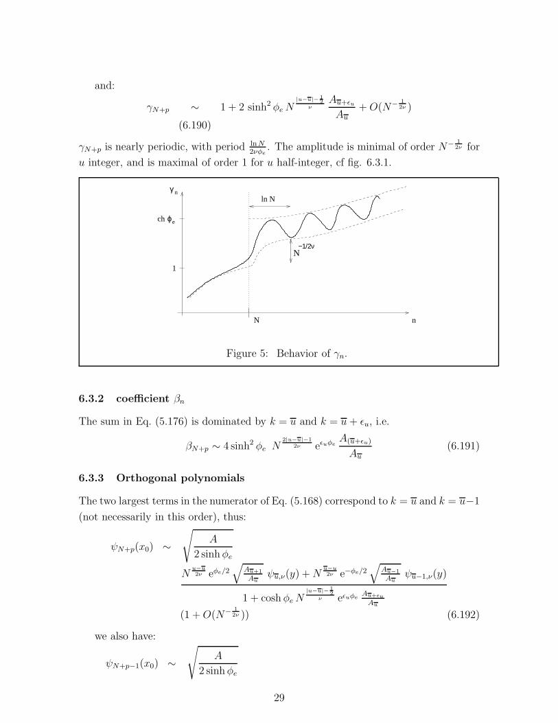
γN+p ∼ 1 + 2 sinh2 φeN|u−u|−1

2ν

Au+ǫu

Au+O(N− 1

2ν )

(6.190)

γN+p is nearly periodic, with period lnN2νφe

. The amplitude is minimal of order N− 12ν for

u integer, and is maximal of order 1 for u half-integer, cf fig. 6.3.1.

N−1/2ν

nγ

ch ϕe

n

ln N

N

1

Figure 5: Behavior of γn.

6.3.2 coefficient βn

The sum in Eq. (5.176) is dominated by k = u and k = u+ ǫu, i.e.

βN+p ∼ 4 sinh2 φe N2|u−u|−1

2ν eǫuφeA(u+ǫu)

Au

(6.191)

6.3.3 Orthogonal polynomials

The two largest terms in the numerator of Eq. (5.168) correspond to k = u and k = u−1

(not necessarily in this order), thus:

ψN+p(x0) ∼√

A

2 sinhφe

Nu−u2ν eφe/2

√

Au+1

Auψu,ν(y) +N

u−u2ν e−φe/2

√

Au−1

Auψu−1,ν(y)

1 + cosh φeN|u−u|−1

2ν eǫuφe

Au+ǫu

Au

(1 +O(N− 12ν )) (6.192)

we also have:

ψN+p−1(x0) ∼√

A

2 sinhφe

29

Nu−u2ν e−φe/2

√

Au+1

Auψu,ν(y) +N

u−u2ν eφe/2

√

Au−1

Auψu−1,ν(y)

1 + coshφeN|u−u|− 1

2ν e−ǫuφe

Au+ǫu

Au

(1 +O(N− 12ν )) (6.193)

6.3.4 Hilbert transforms

Similarly, using Eq. (5.172), we find that the Hilbert transform of the orthogonal

polynomial πn, are asymptoticaly given by:

φN+p−1(x0) ∼√

A

2 sinhφe

Nu−u2ν e−φe/2

√

Au+1

Auφu,ν(y) +N−u−u

2ν eφe/2√

Au−1

Auφu−1,ν(y)

1 + coshφeN2|u−u|−1

2ν e−ǫuφeAu+ǫu

Au

(6.194)

and

φN+p(x0) ∼√

A

2 sinhφe

Nu−u2ν eφe/2

√

Au+1

Auφu,ν(y) +N−u−u

2ν e−φe/2√

Au−1

Auφu−1,ν(y)

1 + cosh φeN2|u−u|−1

2ν eǫuφeAu+ǫu

Au

(6.195)

6.3.5 Matrix form

The matrix:

Ψn(x) =

(

ψn−1(x) φn−1(x)ψn(x) φn(x)

)

(6.196)

is in that regime (u ≥ 0):

Ψn(x) ∼√

A

2 sinhφeL−1

(

e12φe e−

12φe

e−12φe e

12φe

)

R

(

ψu−1,ν(y) φu−1,ν(y)ψu,ν(y) φu,ν(y)

)

(6.197)

where

R = diag

(

N−u−u2ν

√

Au−1

Au

, Nu−u2ν

√

Au+1

Au

)

(6.198)

L = 1 + coshφeN2|u−u|−1

2νAu+ǫu

Au

(

e−ǫuφe 00 eǫuφe

)

(6.199)

30

6.3.6 Kernel

The kernel Kn(x, x′) is given by the Christioffel–Darboux formula:

Kn(x, x′) = γnψn(x)ψn−1(x

′) − ψn(x′)ψn−1(x)

x− x′(6.200)

We find:

Kn(x, x′) ∼ N12ν A

4 sinh2 φe

γu,νψu,ν(y)ψu−1,ν(y

′) − ψu−1,ν(y)ψu,ν(y′)

(y − y′)(6.201)

i.e.

Kn(x, x′) ∼ Ku,ν(y, y′)dy

dx(6.202)

6.3.7 Large u limit

Using Stirling’s formula (cf appendix H), we find that for large u, all those asymptotics

match with the classical limit of section 4.4.

7 Conclusion

We have computed the asymptotics of orthogonal polynomials in the birth of a cut

critical limit. This corresponds to the appearance of a new connected component for

the support of the eigenvalue density, away from other cuts.

We have found some universal behaviour, which depends only on the degree ν of

vanishing of the density at the new cut, and 2 coshφe which parametrizes the distance

between the new cut and the old cut. The parametrix near the new cut, is simply

the system corresponding to a model matrix model in the potential x2ν , and with

u = [12

+ 2νφen−NlnN

] eigenvalues.

This new universal behaviour does not seem to correspond to a conformal field

theory (unlike previously known critical behaviours), because the exponent of N is not

constant.

It would be interesting to complete the “physicist’s proof” presented here, with a

mathematical one, for instance using Riemann-Hilbert metods as in [2, 11].

Aknowledgements

We would like to thank Pavel Bleher for initiating this work and for many discussions,

we also want to thank B. Dubrovin, T. Grava, I. Kostov, H. Saleur, A. Zamolodchikov,

for fruitful discussions on those subjects. This work is partly supported by the Enigma

european network MRT-CT-2004-5652, by the ANR project Geometrie et integrabilite

en physique mathematique ANR-05-BLAN-0029-01, and by the Enrage european net-

work MRTN-CT-2004-005616.

31

Appendix H Stirling formula and other asymp-

totics

Stirling formula:

n! ∼ nne−n√

2πn(1 +1

12n+ . . .) (H.1)

from which we deduce:

ln (1 . . . (n− 1)!) ∼ 1

2n2 lnn− 3

4n2 +

n

2ln 2π − 1

12lnn+O(1) (H.2)

and

lnHn ∼ n ln 2π − lnn

12+ . . . (H.3)

Asymptotics of ζk,ν. For large k we have:

ln ζk,ν ∼ k2

2νln k − 3

4νk2 +

k

νln k +O(k) (H.4)

Appendix I Elliptical functions

We introduce a few definitions about elliptical functions [24]: The elliptical sine func-

tion sn(u,m) is defined by the following identity:

u =

∫ sn(u,m)

0

dy√

(1 − y2)(1 −my2)(I.1)

The complete integrals are defined by:

K(m) :=

∫ 1

0

dy√

(1 − y2)(1 −my2)(I.2)

K ′(m) := K(1 −m) =

∫ ∞

0

dy√

(1 + y2)(1 +my2)(I.3)

E(u,m) :=

∫ sn(u,m)

0

√

1 −my2

1 − y2dy (I.4)

E(m) :=

∫ 1

0

√

1 −my2

1 − y2dy , E ′(m) := E(1 −m) (I.5)

When m→ 0 one has:

K ∼ π

2

(

1 +m

4+

9m2

64+ . . .+O(m3)

)

K ′ ∼ ln1√m

(

1 +m

4+

9m2

64+ . . .+O(m3)

)

32

E ∼ π

2

(

1 − m

4− 3m2

64+ . . .+O(m3)

)

E ′ ∼ 1 − m

2ln

1√m

+O(m2)

(I.6)

References

[1] P. Bleher and A. Its, Double scaling limit in the matrix model: the Riemann-

Hilbert approach, Preprint, 2002, (arXiv:math-ph/0201003).

[2] P. Bleher, A. Its, “Semiclassical asymptotics of orthogonal polynomials, Riemann-

Hilbert problem, and universality in the matrix model” Ann. of Math. (2) 150,

no. 1, 185–266 (1999).

[3] P. Bleher, B. Eynard, ”Double scaling limit in random matrix models and a non-

linear hierarchy of differential equations”, J. Phys. A36 (2003) 3085-3106, xxx,

hep-th/0209087.

[4] G. Bonnet, F. David, B. Eynard, Breakdown of universality in multi-cut matrix

models, J.Phys. A: Math. Gen. 33 (2000) 6739-6768.

[5] E. Brezin, C. Itzykson, G. Parisi, and J. Zuber, Comm. Math. Phys. 59, 35 (1978).

[6] G.M.Cicuta “Phase transitions and random matrices”, cond-mat/0012078.

[7] C. Crnkovic, M. Douglas, and G. Moore. Loop equations and the topological phase

of multi-cut matrix models, Int. J. Mod. Phys. A7 (1992) 7693-7711.

[8] J.M. Daul, V. Kazakov, I.K. Kostov, “Rational Theories of 2D Gravity from the

Two-Matrix Model”, Nucl. Phys. B409, 311-338 (1993), hep-th/9303093.

[9] F. David, “Planar diagrams, two-dimensional lattice gravity and surface models”,

Nucl. Phys. B 257 [FS14] 45 (1985).

[10] P. Deift, Orthogonal Polynomials and Random Matrices: a Riemann-Hilbert Ap-

proach, Courant (New York University Press, ., 1999).

[11] P. Deift, T. Kriecherbauer, K. T. R. McLaughlin, S. Venakides, Z. Zhou, “Uni-

form asymptotics for polynomials orthogonal with respect to varying exponential

weights and applications to universality questions in random matrix theory”, Com-

mun. Pure Appl. Math. 52, 1335–1425 (1999).

33

[12] K. Demeterfi, N. Deo, S. Jain, and C.-I Tan, Multiband structure and critical

behavior of matrix models, Phys. Rev. D, 42 (1990) 4105-4122.

[13] P. Di Francesco, P. Ginsparg, J. Zinn-Justin, “2D Gravity and Random Matrices”,

Phys. Rep. 254, 1 (1995).

[14] Di Ffrancesco P., Mathieu P., Senechal D., “Conformal Field Theory”; Corr. 2nd

printing, 1998 (Springer-Verlag, Heidelberg, New York, 1997) Graduate Texts in

Contemporary Physics.

[15] F.J. Dyson, ”Correlations between the eigenvalues of a random matrix”, Comm.

Math. Phys. 19 (1970) 235-250.

[16] N. Ercolani K. Mac Laughlin, ”Asymptotics of the partition function for random

matrices via Riemann–Hilber technics and applications to graphical enumeration”,

IMRN 22003, no 14, 755-820.

[17] H.M. Farkas, I. Kra, ”Riemann surfaces” 2nd edition, Springer Verlag, 1992.

[18] J. Fay, ”Theta Functions on Riemann Surfaces”, Lectures Notes in Mathematics,

Springer Verlag, 1973.

[19] K. Johansson, On fluctuations of eigenvalues of random hermitian matrices, Duke

Math. J. 91 (1988), 151–204.

[20] M.L. Mehta, Random Matrices, 2nd edition, (Academic Press, New York, 1991).

[21] V. Periwal and D. Shevitz, Exactly solvable unitary matrix models: multicritical

potentials and correlations, Nucl. Phys. B 333 (1990), 731–746.

[22] G. Szego. Orthogonal Polynomials, 3rd ed. AMS, Providence, 1967.

[23] C. Tracy and H. Widom, Introduction to random matrices. In: Geometric and

quantum aspects of integrable systems (Scheveningen, 1992), Lecture Notes in

Phys. 424, Springer-Verlag, Berlin, 1993, 103-130.

[24] Special Functions, Wang Z.X., Guo D.R., World Scientific, 1989.

34