ECE541: Stochastic Signals and Systems Fall 2018

Chapter 8: Random Processes

Dr. Salim El Rouayheb

1 Random Process

Definition 1. A discrete random process X(n), also denoted as Xn, is an infinite sequence ofrandom variables X1, X2, X3, . . . ; we think of n as the time index.

1. Mean function: µX(n) = E[X(n)].

2. Auto-correlation function: RXX(k, l) = E[X(k)X(l)].

3. Auto-covariance function: KXX(k, l) = RXX(k, l)− µX(k)µX(l).

Definition 2. X(n) is a Gaussian r.p. if Xi1 , Xi2 , . . . , Xim are jointly Gaussian for any m ≥ 1.

Example 1. Let W (n) be an i.i.d Gaussian r.p with autocorrelation RWW (k, l) = σ2δ(k − l) andmean µW (n) = 0 ∀n, where

δ(x− a) =

{1 x = a,

0 otherwise.

⇒ RWW (k, l) = E [WkWl] =

{σ2 k = l,

0 otherwise.

Which means that for l = k,

RW (k, l) = E[W 2l ] = V [Wl] = σ2,

and Wl & Wk are correlated. While for l 6= k,

RW (k, l) = 0,

and Wl & Wk are uncorrelated and therefore independent because they are jointly Gaussian.

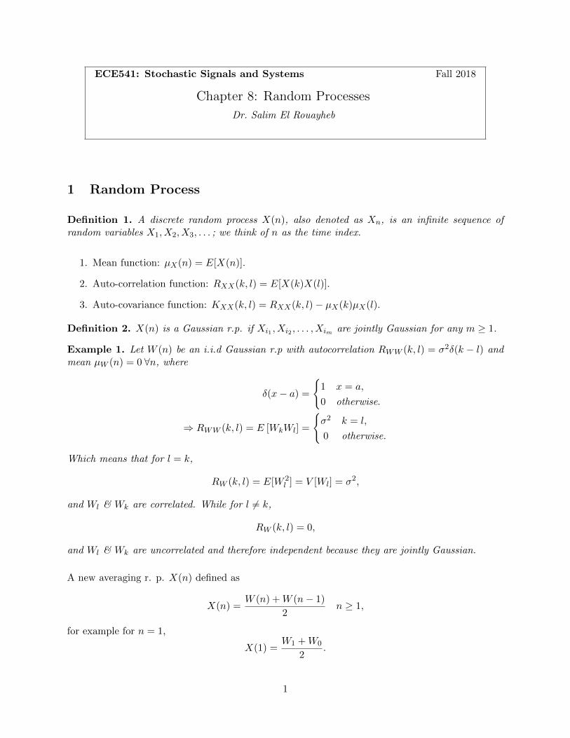
A new averaging r. p. X(n) defined as

X(n) =W (n) +W (n− 1)

2n ≥ 1,

for example for n = 1,

X(1) =W1 +W0

2.

1

0 1 2 3 4 5 6 7

−2

0

2

n

Xn

0 1 2 3 4 5 6 7

−4

−2

0

2

4

n

Wn

Figure 1: A possible realization of the random process W (n) and its corresponding averaging functionX(n).

.

Questions:

1. What is the pdf of X(n)?

2. Find the autocorrelation function RXX(k, l)

Answers:

1. From previous chapters we know that X(n) is a Gaussian r.v. because it is a linear combi-nation of Gaussian r.v. Hence, it is enough to find the mean and variance of Xn to find itspdf.

E [X(n)] = E

[1

2(Wn +Wn−1)

],

=1

2(E [Wn] + E [Wn−1]) ,

= 0.

V [X (n)] = V

[1

2(Wn +Wn−1)

],

=1

4(V [Wn] + V [Wn−1]) because Wn & Wn−1 are independent,

=1

4

(σ2 + σ2

),

=σ2

2.

2

OR:

V [X (n)] = E[X2n

]− µ2

Xn, (1)

= E

[1

4(Wn +Wn−1)2

], (2)

=1

4

(E[W 2n

]+ E

[W 2n−1

]+ 2E [WnWn−1]

), (3)

=1

4

(σ2 + σ2

), (4)

=σ2

2, (5)

where equation (4) follows from the fact that

E [WnWn−1] = RWW (n, n− 1) = 0.

Therefore,

fXn(xn) =1√

2π σ√2

exp

(− x2

n

2σ2

2

),

=1

σ√π

exp

(−x

2n

σ2

).

2. Before we apply the formula, let us try to find the autocorrelation intuitively. By definition:

X1 =W1 +W0

2, X2 =

W2 +W1

2, X3 =

W3 +W2

2.

It is clear that X1 and X3 are uncorrelated (independent) because they do not have any Wi

in common and W (n) is i.i.d. However, X1, X2 and X2, X3 are correlated.

RXX(k, l) = E [XkXl] ,

=1

4E [(Wk +Wk−1) (Wl +Wl−1)] ,

=1

4(E [WkWl] + E [WkWl−1] + E [Wk−1Wl] + E [Wk−1Wl−1]) .

Recall from the definition of W (n) that

E [WkWl] =

{σ2/2 k = l,

0 otherwise,E [WkWl−1] =

{σ2/4 k = l − 1,

0 otherwise,

E [Wk−1Wl] =

{σ2/4 k = l + 1,

0 otherwise,E [Wk−1Wl−1] =

{σ2/2 k = l,

0 otherwise.

Therefore,

RXX(k, l) =

σ2

2 k = l,σ2

4 k = l ± 1,

0 otherwise.

3

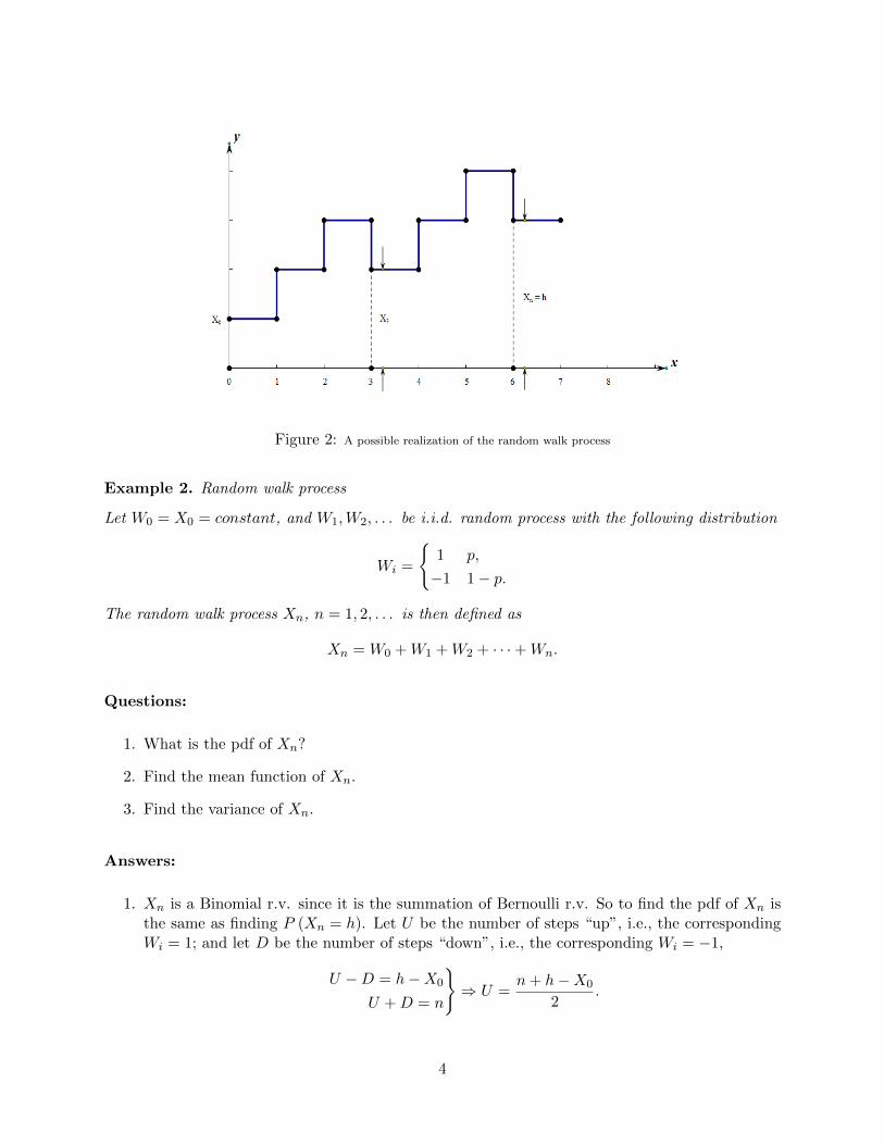
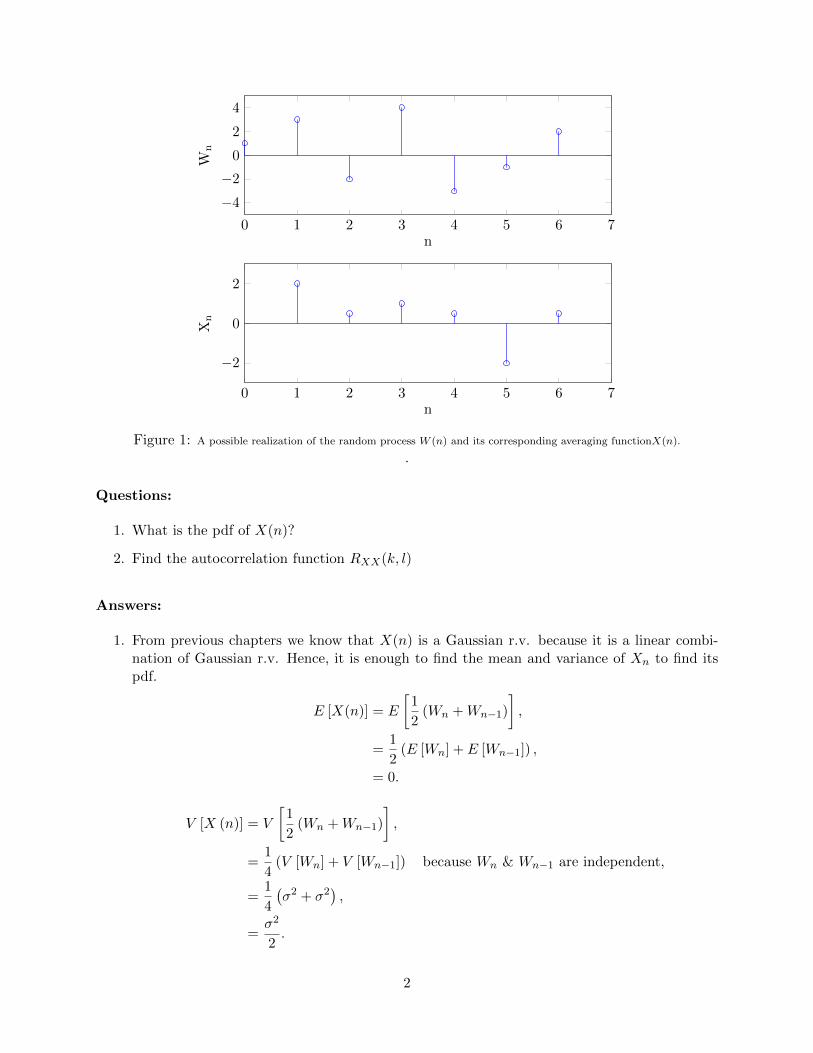
Figure 2: A possible realization of the random walk process

Example 2. Random walk process

Let W0 = X0 = constant, and W1,W2, . . . be i.i.d. random process with the following distribution

Wi =

{1 p,

−1 1− p.

The random walk process Xn, n = 1, 2, . . . is then defined as

Xn = W0 +W1 +W2 + · · ·+Wn.

Questions:

1. What is the pdf of Xn?

2. Find the mean function of Xn.

3. Find the variance of Xn.

Answers:

1. Xn is a Binomial r.v. since it is the summation of Bernoulli r.v. So to find the pdf of Xn isthe same as finding P (Xn = h). Let U be the number of steps “up”, i.e., the correspondingWi = 1; and let D be the number of steps “down”, i.e., the corresponding Wi = −1,

U −D = h−X0

U +D = n

}⇒ U =

n+ h−X0

2.

4

Then,

P (Xn = h) =

(n

U

)pU (1− p)n−U ,

=

(n

n+h−X02

)p

n+h−X02 (1− p)

n−h+X02 .

Remark 1. if n >>>(n is big enough), Xn ∼ N(., .) by CLT.

2.

E [Xn] = E [X0] + E [W1] + · · ·+ E [Wn] ,

= X0 + n (1× p+ (−1)(1− p)) ,= X0 + (2p− 1)n.

Leading to the following for different values of p:

if p =1

2, E [Xn] = X0,

if p >1

2, E [Xn] −−−→

n→∞+∞,

if p <1

2, E [Xn] −−−→

n→∞−∞.

3.

V [Xn] = V [X0] + V [W1] + · · ·+ V [Wn] , (6)

= 0 + 4np(1− p), (7)

= 4np(1− p). (8)

Where equation (6) is applicable because W (n), n = 1, 2, . . . , are i.i.d.

Remark 2. By CLT, when n→∞,

limn→∞

FXn(xn) =

∫ xn

−∞

exp(− (xn−(x0+(2p−1)n))2

2(4np(1−p))

)√

2π√

4np(1− p)dxn,

=

∫ xn

−∞

exp(− (xn−x0)2

2n

)√

2πndxn, (for p =

1

2).

2 Brief review on the random walk process

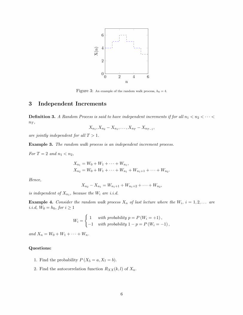
Recall that the random walk process is a process that starts from a point X0 = h0. At each timeinstant n, Xn = Xn−1 ± 1 (c.f. fig. 3 for an example).

5

0 2 4 60

2

4

6

n

X(n

)Figure 3: An example of the random walk process, h0 = 4.

3 Independent Increments

Definition 3. A Random Process is said to have independent increments if for all n1 < n2 < · · · <nT ,

Xn1 , Xn2 −Xn1 , . . . , XnT −XnT−1 ,

are jointly independent for all T > 1.

Example 3. The random walk process is an independent increment process.

For T = 2 and n1 < n2,

Xn1 = W0 +W1 + · · ·+Wn1 ,

Xn2 = W0 +W1 + · · ·+Wn1 +Wn1+1 + · · ·+Wn2 .

Hence,Xn2 −Xn1 = Wn1+1 +Wn1+2 + · · ·+Wn2 ,

is independent of Xn1, because the Wi are i.i.d.

Example 4. Consider the random walk process Xn of last lecture where the Wi, i = 1, 2, . . . arei.i.d, W0 = h0, for i ≥ 1

Wi =

{1 with probability p = P (Wi = +1) ,

−1 with probability 1− p = P (Wi = −1) ,

and Xn = W0 +W1 + · · ·+Wn.

Questions:

1. Find the probability P (X5 = a,X7 = b).

2. Find the autocorrelation function RXX(k, l) of Xn.

6

Answers:

1. Recall from example 2 of last lecture that we can compute P (Xn = h) using the binomialformula derived there. The first method to answer this question is by using Bayes’ rule:

P (X5 = a,X7 = b) = P (X5 = a)P (X7 = b|X5 = a) ,

= P (X5 = a)P (X7 −X5 = b− a) ,

= P (X5 = a)P (X2 −X0 = b− a) ,

= P (X5 = a)P (X2 = b− a+X0) ,

And the second method is by using the independent increment property of the random walkprocess as follows:

P (X5 = a,X7 = b) = P (X5 = a,X7 −X5 = b− a) , (9)

= P (X5 = a)P (X7 −X5 = b− a) . (10)

Equation (10) follows from the independent increment property.

2. Now we can use this to find the autocorrelation function, assuming without loss of generalitythat l > k.

RXX(k, l) = E[x(k)2],

= E[(W0 +W1 + · · ·+Wk)

2],

= E[W 2

0 +W 21 + · · ·+W 2

k + 2 (W0W1 + · · ·+WkWk−1)],

= E[W 2

0

]+ kE

[W 2

1

]+ 2h0 (E [W1] + · · ·+ E [Wk]) + 2E [W1W2 + · · ·+Wk−1Wk] ,

= h20 + k + 2h0(2p− 1) + 2

k(k − 1)

2(2p− 1)2.

For p = 12 ,

RXX(k, l) =

{h2

0 + k l > k,

h20 + l l < k.

⇒ RXX(k, l) = h20 + min(k, l).

Practice 1. Try to find at home RXX(k, l) in a different way, i.e., using

RXX(k, l) = [(W1 +W2 + · · ·+Wk) (W1 +W2 + · · ·+Wl)] .

Definition 4. A random process X(t) is stationary if it has the same nth-order CDF as X(t+T ),that is, the two n-dimensional functions

FX(x1, . . . , xn; t1, . . . , tn) = FX(x1, . . . , xn; t1 + T, . . . , tn + T )

are identically equal for all T , for all positive integers n, and for all t1, . . . , tn.

Example 5. Consider the i.i.d. Gaussian r.p. W1,W2, . . . from last lecture.

Wi ∼ N(0, σ2) ∀ i ≥ 1.

7

−10 −5 0 5 10 15−2

−1

0

1

2

n

X(n

)

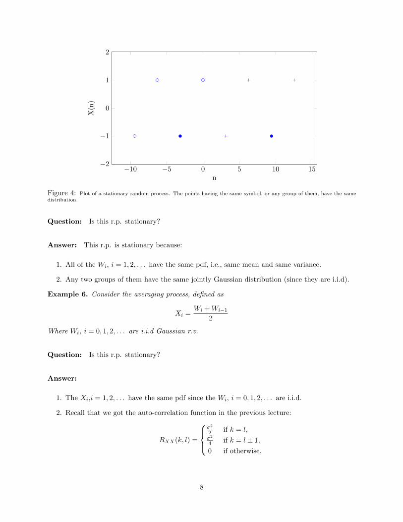
Figure 4: Plot of a stationary random process. The points having the same symbol, or any group of them, have the samedistribution.

Question: Is this r.p. stationary?

Answer: This r.p. is stationary because:

1. All of the Wi, i = 1, 2, . . . have the same pdf, i.e., same mean and same variance.

2. Any two groups of them have the same jointly Gaussian distribution (since they are i.i.d).

Example 6. Consider the averaging process, defined as

Xi =Wi +Wi−1

2

Where Wi, i = 0, 1, 2, . . . are i.i.d Gaussian r.v.

Question: Is this r.p. stationary?

Answer:

1. The Xi,i = 1, 2, . . . have the same pdf since the Wi, i = 0, 1, 2, . . . are i.i.d.

2. Recall that we got the auto-correlation function in the previous lecture:

RXX(k, l) =

σ2

2 if k = l,σ2

4 if k = l ± 1,

0 if otherwise.

8

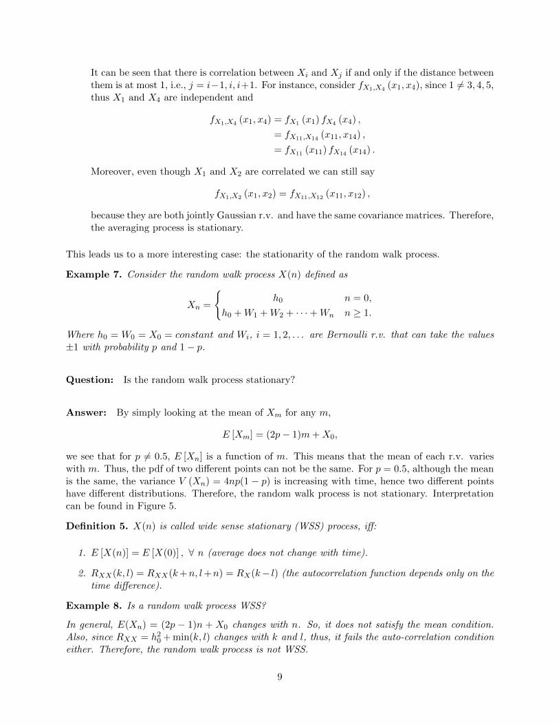
It can be seen that there is correlation between Xi and Xj if and only if the distance betweenthem is at most 1, i.e., j = i−1, i, i+1. For instance, consider fX1,X4 (x1, x4), since 1 6= 3, 4, 5,thus X1 and X4 are independent and

fX1,X4 (x1, x4) = fX1 (x1) fX4 (x4) ,

= fX11,X14 (x11, x14) ,

= fX11 (x11) fX14 (x14) .

Moreover, even though X1 and X2 are correlated we can still say

fX1,X2 (x1, x2) = fX11,X12 (x11, x12) ,

because they are both jointly Gaussian r.v. and have the same covariance matrices. Therefore,the averaging process is stationary.

This leads us to a more interesting case: the stationarity of the random walk process.

Example 7. Consider the random walk process X(n) defined as

Xn =

{h0 n = 0,

h0 +W1 +W2 + · · ·+Wn n ≥ 1.

Where h0 = W0 = X0 = constant and Wi, i = 1, 2, . . . are Bernoulli r.v. that can take the values±1 with probability p and 1− p.

Question: Is the random walk process stationary?

Answer: By simply looking at the mean of Xm for any m,

E [Xm] = (2p− 1)m+X0,

we see that for p 6= 0.5, E [Xn] is a function of m. This means that the mean of each r.v. varieswith m. Thus, the pdf of two different points can not be the same. For p = 0.5, although the meanis the same, the variance V (Xn) = 4np(1 − p) is increasing with time, hence two different pointshave different distributions. Therefore, the random walk process is not stationary. Interpretationcan be found in Figure 5.

Definition 5. X(n) is called wide sense stationary (WSS) process, iff:

1. E [X(n)] = E [X(0)] , ∀ n (average does not change with time).

2. RXX(k, l) = RXX(k+n, l+n) = RX(k− l) (the autocorrelation function depends only on thetime difference).

Example 8. Is a random walk process WSS?

In general, E(Xn) = (2p − 1)n + X0 changes with n. So, it does not satisfy the mean condition.Also, since RXX = h2

0 + min(k, l) changes with k and l, thus, it fails the auto-correlation conditioneither. Therefore, the random walk process is not WSS.

9

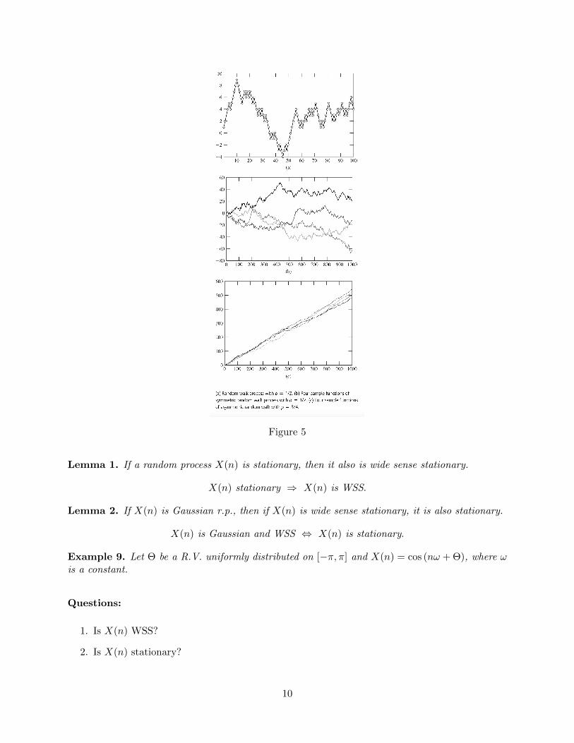
Figure 5

Lemma 1. If a random process X(n) is stationary, then it also is wide sense stationary.

X(n) stationary ⇒ X(n) is WSS.

Lemma 2. If X(n) is Gaussian r.p., then if X(n) is wide sense stationary, it is also stationary.

X(n) is Gaussian and WSS ⇔ X(n) is stationary.

Example 9. Let Θ be a R.V. uniformly distributed on [−π, π] and X(n) = cos (nω + Θ), where ωis a constant.

Questions:

1. Is X(n) WSS?

2. Is X(n) stationary?

10

Answers:

1. To check the Mean Condition:

E [X(n)] =

∫ +∞

−∞fΘ(θ) cos (nω + θ) dθ,

=1

2π

∫ π

−πcos (nω + θ) dθ,

= 0.

It is equal to 0 because the cosine function is symmetric between −π and π. E [X(n)] isconstant for any n, then it satisfies the mean condition.

2. To check the Auto-Correlation Condition:

RXX(k, l) = E [X (k)X (l)] , (11)

=1

2π

∫ +π

−πcos (kω + θ) cos (lω + θ) dθ, (12)

=1

2cos (ω (k − l)) , (13)

= RXX(k − l). (14)

(15)

Where equation (13) can be found after some trigonometric calculations beginning by

cosαcosβ =1

2[cos (α− β) + cos (α+ β)] .

Thus, X(n) is WSS.

3. X(n) is stationary. We will not prove it rigourously, however we will give the main idea.Consider ω = π,

X(n) = cos(nπ + Θ),

X(1) = cos(π + Θ),

X(2) = cos(2π + Θ) = cos(Θ),

X(3) = cos(3π + Θ) = cos(π + Θ),

X(4) = cos(4π + Θ) = cos(Θ).

It is clear that any Xn is uniformly distributed on [−1, 1] because the cosine is symmetricon any interval of length 2π. in particular for Θ ∼ U [−π, π] and Θ′ = Θ + π ∼ U [0, 2π],cos(Θ) ∼ U [−1, 1] and cos(Θ′) ∼ U [−1, 1]. Therefore, the Xn have same distribution andX(n) is stationary.

Generally, since Θ ∼ U [−π, π] and ω is a constant. The r.v. nω+ Θ is uniformly distributedon [nω − π, nω + π] which is an interval of length 2π ⇒ cos (nω + Θ) ∼ U [−1, 1] for all n.Therefore, all the Xn have the same distribution and X(n) is stationary.

11

4 Continuous Time Random Process

Definition 6. A continuous time random process X(t), is a random process defined for any t ∈ R.

We can redefine, in continuous time, everything defined in discrete time.

5 Poisson process

The Poisson process is a special case of a counting process. So first, we will start by defining acounting process.

5.1 Counting process

Definition 7 (Counting process). A counting process is a continuous random process {N(t), t ≥ 0}with values that are non-negative, integer, and non-decreasing:

1. N(t) ≥ 0.

2. N(t) is an integer.

3. If s ≤ t then N(s) ≤ N(t).

Example 10 (Bernoulli process). Let Xi, i = 1, . . . , n be iid Bernoulli random variables withparameter p. Define the Bernoulli process Sn = X1 + . . .+Xn. The Bernoulli process is a discretecounting process because it satisfies the three conditions in Definition 7. Namely,

• Since Xi ∈ {0, 1}, i = 1, . . . , n, then Xi ≥ 0 and Xi is an integer. Therefore, Sn = X1 + . . .+Xn is a non-negative integer.

• For m ≤ n, we have Sn − Sm = Xm+1 + . . .+Xn ≥ 0. Hence, if m ≤ n then Sm ≤ Sn.

Now, we define the Poisson process.

Definition 8 (Poisson process). The Poisson process is a counting process {N(t), t ≥ 0} thatsatisfies the following three properties:

1. N(0) = 0.

2. N(t) has independent incerements, i.e., for t0 < t1 < . . . < tn, the random variables(N(t1)−N(t0)) , (N(t2)−N(t1)) , . . . , (N(tn)−N(tn−1)) are independent.

3. The total count in any interval of length t is a Poisson random variable with parameter (ormean) λt, i.e.,

P (N(t) = k) =(λt)ke−λt

k!, k = 0, 1, 2, . . . .

12

It follows from the Definition 8 that

µN (t) = E [N(t)] = λt,

V (N(t)) = λt.

Moreover, based on the independent increments property we have

P (N(t1) = i,N(t2) = j) = P (N(t1) = i)P (N(t2) = j|N(t1) = i) ,

= P (N(t1) = i)P (N(t2)−N(t1) = j − i) ,= P (N(ti) = i)P (N(t2 − t1) = j − i) ,

=(t1λ)ie−t1λ

i!

((t2 − t1)λ)j−i e−(t2−t1)λ

(j − i)!.

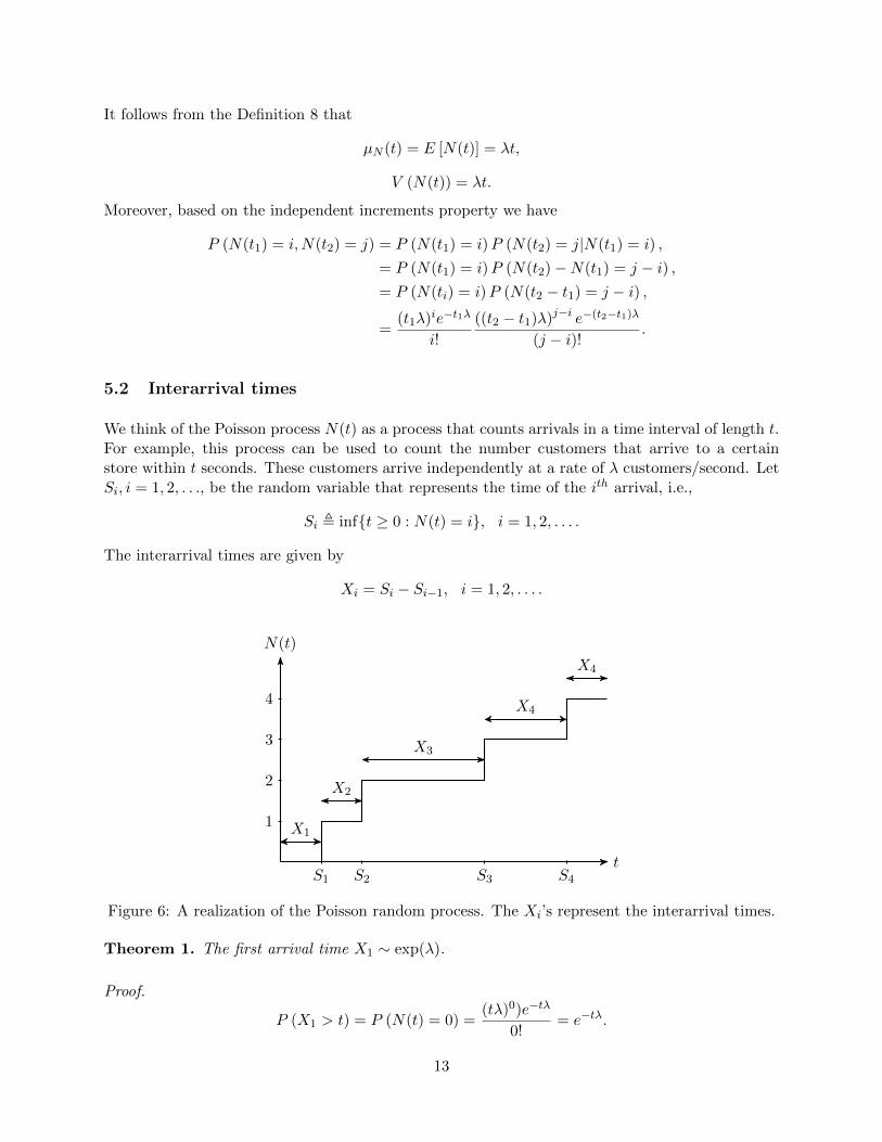
5.2 Interarrival times

We think of the Poisson process N(t) as a process that counts arrivals in a time interval of length t.For example, this process can be used to count the number customers that arrive to a certainstore within t seconds. These customers arrive independently at a rate of λ customers/second. LetSi, i = 1, 2, . . ., be the random variable that represents the time of the ith arrival, i.e.,

Si , inf{t ≥ 0 : N(t) = i}, i = 1, 2, . . . .

The interarrival times are given by

Xi = Si − Si−1, i = 1, 2, . . . .

t

N(t)

S1 S2 S3 S4

1

2

3

4

X1

X2

X3

X4

X4

Figure 6: A realization of the Poisson random process. The Xi’s represent the interarrival times.

Theorem 1. The first arrival time X1 ∼ exp(λ).

Proof.

P (X1 > t) = P (N(t) = 0) =(tλ)0)e−tλ

0!= e−tλ.

13

Therefore,FX1(t) = P (X1 ≤ t) = 1− e−λt.

This is the CDF of an exp(λ) random variable.

Theorem 2. All the interarrival times, Xi, i = 1, 2, . . . , are iid and have a distribution exp(λ).

Proof.

P (Xn+1 > t|X1 = t1, . . . , Xn = tn) = P (Xn+1 > t|S1 = s1, . . . , Sn = sn) ,

where si = t1 + . . .+ ti, for i = 1, . . . , n. Therefore,

P (Xn+1 > t|X1 = t1, . . . , Xn = tn) = P (Xn+1 > t|S1 = s1, . . . , Sn = sn)

= P (Sn+1 > t+ sn|Sn = sn)

= P (N(t+ sn)−N(sn) = 0|Sn = sn)

= P (N(t) = 0|Sn = sn) (independent increments)

= P (N(t) = 0)

= e−λt

= Pr(X1 > t).

Therefore, Xi, i = 1, 2, . . . are iid and have a distribution exp(λ).

5.3 Autocovariance and stationarity of Poisson process

Assume, without loss of generality, that t1 < t2.

KNN (t1, t2) = E [(N(t1)− λt1) (N(t2)− λt2)] ,

= E [(N(t1)− λt1) (N(t2)−N(t1)− λt2 + λt1 +N(t1)− λt1)] ,

= E [(N(t1)− λt1) (N(t2)−N(t1))− (λt2 − λt1)]︸ ︷︷ ︸0

+E[(N(t1)− λt1)2

],

= λt1.

If t2 ≤ t1 then KNN (t1, t2) = λt2. In general, KNN (t1, t2) = λmin (t1, t2).

Question: Is N(t) WSS?

Answer:

1. E [N(t)] = λt, depends on t.

2. KNN (t1, t2) = λmin (t1, t2), depends on t.

Hence N(t) is not WSS.

14

6 Continuous Gaussian Random Process

Definition 9. X(t) is a Gaussian random process if X(t1), X(t2), . . . , X(tk) are jointly Gaussianfor any k, i.e.,

fX(t1),X(t2),...,X(tk) =1

(2π)12 |KXX |

12

exp

(−1

2

(¯X −

¯µX)TK−1XX

(¯X −

¯µx))

.

Example 11. Let X(t) be a Gaussian random process with µX(t) = 3t and KXX = 9e−2|t1−t2|.

Question: Find the pdf of X(3) and Y = X(1) +X(2).

Answer: We know that X(3) is a Gaussian r.v. (by definition of X(t)) and Y is also a Gaussianr.v. being a linear combination of two Gaussian r.v. Therefore, it is enough to find the mean andthe variance of those variables in order to find their PDFs.

1. X(3): µX(3) = 9 and V [X(3)] = 9e−|3−3| = 9. Thus,

fX(3)(x) =1

3√

2πe−

12

(x−9)2

9 .

2. Y :

E [y] = E [X(1)] + E [x(2)] = 3 + 6 = 9,

V [Y ] = V (X(1)) + V [X(2)] + 2cov (X(1), X(2)) ,

cov (X(1), X(2)) = 9e−2|2−1| = 9e−2,

V [Y ] = 9 + 9 + 9e−2 = 18 + 18e−2.

Another way to find the variance is the following:

V [Y ] = E[(X(1) +X(2))2

]− (E [X(1)] + E [X(2)])2 ,

= E[X(1)2

]+ E

[X(2)2

]+ 2E [X(1)X(2)]− E2 [X(1)]− E2 [X(2)]− 2E [X(1)X(2)] ,

= V (X(1)) + V (X(2)) + 2cov (X(1), X(2)) ,

= 9 + 9 + 2× 9e−2,

= 18 + 18e−2.

15