Journal of

Mechanics ofMaterials and Structures

ANALYSIS OF NONSTATIONARY RANDOM PROCESSESUSING SMOOTH DECOMPOSITION

Rubens Sampaio and Sergio Bellizzi

Volume 6, No. 7-8 September–October 2011

mathematical sciences publishers

JOURNAL OF MECHANICS OF MATERIALS AND STRUCTURESVol. 6, No. 7-8, 2011

msp

ANALYSIS OF NONSTATIONARY RANDOM PROCESSESUSING SMOOTH DECOMPOSITION

RUBENS SAMPAIO AND SERGIO BELLIZZI

Orthogonal decompositions provide a powerful tool for stochastic dynamics analysis. The most populardecomposition is the Karhunen–Loève decomposition (KLD), also called proper orthogonal decomposi-tion. KLD is based on the eigenvectors of the correlation matrix of the random field. Recently, a modifiedKLD called smooth Karhunen–Loève decomposition (SD) has appeared in the literature. It is based on ageneralized eigenproblem defined from the covariance matrix of the random process and the covariancematrix of the associated time-derivative random process. SD appears to be an interesting tool to extendmodal analysis. Although it does not satisfy the optimality relation of KLD, and maybe is not as gooda candidate for building reduced models as KLD is, SD gives access to the modal vectors independentlyof the mass distribution. In this paper, the main properties of SD for nonstationary random processes areexplored. A discrete nonlinear system is studied through its linearization, for uncorrelated and correlatedexcitation, and the SD of the nonlinear system and of the linearization are compared. It seems that SDdetects not only mass inhomogeneities but also nonlinearities.

1. Introduction

The Karhunen–Loève decomposition (KLD) method has been extensively used as a tool for analyzingrandom fields [Holmes et al. 1996; Lin et al. 2002; Wolter et al. 2002; Kerschen et al. 2005]. KLD revealssome coherent structures which have been advantageously used in different domains such as, for example,the stochastic finite elements method, simulation of random fields, modal analysis of nonlinear systems,and construction of reduced-order models. Depending on the discipline and the properties of the randomfield under study, but also on the averaging operator used to build the KLD [Bellizzi and Sampaio 2006;2007], this decomposition has been called principal component analysis, singular value decomposition(these two in finite dimensions), and proper orthogonal decomposition. In the definition of KLD thereare two inner products, one given by the normalization condition involving the standard inner productand another by the correlation; the latter, like the former, is a symmetric operator. Orthogonality is meantwith respect to the normalization condition. In structural vibration, KLD has been principally applied tothe displacement field, but it can be applied also to the velocity, acceleration, and displacement-velocityfields [Bellizzi and Sampaio 2009a].

Recently, a new multivariable data analysis method called smooth orthogonal decomposition (SOD)has been proposed [Chelidze and Zhou 2006]. SOD is defined from a maximization problem associatedwith a scalar time series of measurement but subject to a minimization constraint acting on the associated

The authors gratefully acknowledge the financial support of CNPq, Faperj, and the cooperation project 672/10 financed byCAPES and COFECUB..Keywords: smooth decomposition, output only modal analysis, linear and nonlinear systems.

1137

1138 RUBENS SAMPAIO AND SERGIO BELLIZZI

time derivative of the time series. SOD can be used to extract normal modes and natural frequencies ofmulti-degree of freedom vibration systems [Zhou 2006]. Free and forced sinusoidal responses have beenconsidered in [Chelidze and Zhou 2006] and randomly excited systems have been analyzed in [Farooqand Feeny 2008]. SOD has been formulated in term of a smooth Karhunen–Loève decomposition (SKLD)to analyze time-continuous stationary random processes in [Bellizzi and Sampaio 2009b]. The SKLD isobtained solving a generalized eigenproblem defined from the covariance matrix of the random processand the covariance matrix of its time derivative. In this paper the SKLD will be referred to as smoothdecomposition (SD) since it neither has the properties of a Karhunen–Loève decomposition nor is itorthogonal in the sense of the standard inner product. There is, indeed, orthogonality with respect toinner products defined by the two correlations, displacement and velocity, as we shall see.

This work presents and discusses a nontrivial generalization of SD for time-continuous nonstationaryrandom processes. This generalization is based on an averaging operator combining the temporal meanand mathematical expectation to build the covariance matrices of the random process and of its timederivative.

This paper is organized as follows: Section 2 extends the SD for nonstationary processes, Section 3extends the proprieties of the SD for the nonstationary case, Section 4 gives a mechanical interpretationof the SD, Section 5 shows some numerical examples, and, finally, Section 6 presents some conclusions.

2. Smooth decomposition

Our goal here is to extend to nonstationary time processes the smooth decomposition introduced in [Bel-lizzi and Sampaio 2009b] as a smooth Karhunen–Loève decomposition for stationary random processes.

Let {U(t), t 2 R} be a Rn-valued random process indexed by R. We assume that {U(t), t 2 R} is asecond-order process and admits a time-derivative process {U(t), t 2 R} which is also a second-orderprocess. With these assumptions, the covariance matrices of {U(t), t 2 R} and {U(t), t 2 R}, denotedRU (t) = E(U(t)TU(t)) and RU (t) = E(U(t)T U(t)), respectively, are time dependent. Without loss ofgenerality, we will also assume that {U(t), t 2 R} is a zero-mean random process and that RU (t) andRU (t) are symmetric positive definite.

In the case of stationary processes (that is, RU (t) and R •U(t) do not depend on time), the smooth

decomposition of {U(t), t 2 R} is defined (see [Bellizzi and Sampaio 2009b]) recursively by the maximumoptimization problem

max02Rn

E( U(t), 0 2)

E( U(t), 0 2), (2-1)

where denotes the inner product in Rn .In the case of nonstationary processes, the objective function (see (2-1)) is time dependent and as in

[Bellizzi and Sampaio 2006], where KLD has been proposed for nonstationary random processes, thetime variable has to be included in the averaging operation. Let ti and t f be two positive constants withti < t f . The ratio

1t f �ti

Z t f

tiE( U(t), 0 2)dt

1t f �ti

Z t f

tiE( U(t), 0 2)dt

(2-2)

ANALYSIS OF RANDOM PROCESSES USING SMOOTH DECOMPOSITION 1139

can be considered to define the smooth decomposition. The objective function (2-2) can be written

0T Rti ,t fU 0

0T Rti ,t f

U 0, (2-3)

where

Rti ,t fU = 1

t f �ti

Z t f

tiRU (t)dt, R

ti ,t f

U = 1t f �ti

Z t f

tiRU (t)dt, (2-4)

showing that the quotient depends on the covariance matrices of {U(t), t 2 [t f , ti ]} and {U(t), t 2 [t f , ti ]}.The vectors that yield the extrema of

max02Rn

0T Rti ,t fU 0

0T Rti ,t f

U 0(2-5)

are solutions of the eigenproblem

Rti ,t fU 0k = �kR

ti ,t f

U 0k . (2-6)

The SD of the random process will then be given by

U(t) =nX

k=1

⇣k(t)0k, (2-7)

where the vectors 0k solve the generalized eigenproblem (2-6) and the scalar random processes, ⇣k(t),are given by

⇣k(t) = 0Tk R

ti ,t fU U(t)

0Tk R

ti ,t fU 0k

= 0Tk R

ti ,t f

U U(t)

0Tk R

ti ,t f

U 0k. (2-8)

Note that the scalar processes {⇣k(t)} can be defined from either Rti ,t fU or Rti ,t f

U ; that is, they do notdepend on which of these two covariance matrices is used.

The following notation is used: the eigenvalues �k are called the smooth values (SVs) (6 = diag(�k)),the eigenvectors 0k are called the smooth modes (SMs) (0 = [0101 · · · 0n]), and the scalar randomprocesses {⇣k(t)} are called the smooth components (SCs). All these quantities depend on the timeinterval [ti , t f ].

The generalized eigenproblem (2-6) is a temporal version (for nonstationary random processes) ofthe generalized eigenvalue problem introduced in [Bellizzi and Sampaio 2009b] to characterize the SDof the stationary process. In addition, in the definition (2-6) only the generalized covariance matricesRti ,t f

U and Rti ,t fU are used, no other operator is necessary. It is important (and trivial) to note that, if

the random process is stationary, the covariance matrices reduce to the stationary ones (as described in[Bellizzi and Sampaio 2009b]) and, if the vector signal is deterministic, the covariance matrices reduce tothe time-average ones (as described in [Chelidze and Zhou 2006]). We will show that the results are, ofcourse, similar to the ones presented in [Chelidze and Zhou 2006; Farooq and Feeny 2008; Bellizzi andSampaio 2009b], but now, since one relies on the covariance matrices, one has a powerful computationtool not available before (see, for example, [Quaranta et al. 2008]).

Finally, the quotient used to define the SD differs significantly from that used to define the classicalKarhunen–Loève decomposition [Bellizzi and Sampaio 2006]. In the SD case, the denominator takes

1140 RUBENS SAMPAIO AND SERGIO BELLIZZI

the covariance matrix of the time-derivative process {U(t), t 2 R} into account which justifies the namesmooth decomposition since the idea is to have a small rate-of-variation of the process.

3. Some properties of smooth decomposition

The classical properties as established in the case of stationary processes [Bellizzi and Sampaio 2009b]are extended to the nonstationary case.

3A. Properties of SV, SM, and SC. The matrices Rti ,t fU and Rti ,t f

U being symmetric positive definiteimplies that all the SVs (eigenvalues) ⌫k are strictly positive and the set of the vectors 0k (the SMs)constitutes a basis which is orthogonal with respect to both covariance matrices Rti ,t f

U and Rti ,t fU . Note

that the SMs are unique up to a scaling constant.The scalar processes {⇣k(t), t 2 R} are correlated:

1t f �ti

Z t f

tiE(⇣k(t)⇣l(t))dt = 0T

k Rti ,t fU R

ti ,t fU R

ti ,t fU 0l

0Tk R

ti ,t fU 0k0

Tl R

ti ,t fU 0l

= 0Tk R

ti ,t f

U Rti ,t f

U Rti ,t f

U 0l

0Tk R

ti ,t f

U 0k0Tl R

ti ,t f

U 0l. (3-1)

So, the SVs are not related to energy distribution and, of course, the SD does not satisfy the standardoptimality relationship as the Karhunen–Loève decomposition does. So, properly speaking, the SD isnot a Karhunen–Loève decomposition. The introduction of regularity has then its drawbacks.

3B. Linear transformation of the SD. Let {V (t), t 2 [ti , t f ]} be a Rn-valued random process defined as

V (t) = AU(t), (3-2)

where A is an invertible matrix.From the relations RV (t) = ARU (t)AT and RV (t) = ARU (t)AT it can be shown that the SVs of

{V (t), t 2 [ti , t f ]} coincide with the SVs of {U(t), t 2 [ti , t f ]} and the sets of the SMs satisfy

0k(V ) = A�T 0k(U ), (3-3)

where 0k(U ) (respectively, 0k(V )) denotes a SM of {U(t), t 2 [ti , t f ]} (respectively, of {V (t), t 2 [ti , t f ]}).Finally, following (2-8), the SCs are invariant with respect to linear change of variables if and only ifAAT = I .

4. Mechanical interpretation of the SD

4A. Discrete linear case. Consider a discrete mechanical system with n degrees of freedom. Let U(t)be the displacement vector at instant t . We assume that U(t) satisfies the initial-value problem

MU(t) + CU(t) + K U(t) = F(t), t 2 [0, t f ], (4-1)

U(0) = U0, U(0) = U0, (4-2)

where M , C , and K are symmetric square matrices with dimensions n ⇥n. The vectors U0 and U0 definethe initial conditions of the motion at t = 0, and {F(t), t 2 [0, t f ]} is a random vector process. Withoutloss of generality, we have assumed that ti = 0.

ANALYSIS OF RANDOM PROCESSES USING SMOOTH DECOMPOSITION 1141

The linear normal modes (LNM) are classically defined from the free responses of the associatedundamped system as

K8 = M8�2,

where 8 = [81 · · · 8i · · · 8n] denotes the modal matrix with the normalization condition 8T M8 = I whichimplies that 8T K8 = �2 = diag(!2

i ) (!2i and 8i denote the squared resonance frequencies and the asso-

ciated normal-mode vectors).Here we focus on (4-1) with proportional damping. Note that in this case the matrix 8TC8 is also

diagonal. In this section the aim is to establish when and how the SMs and the SVs, defined in Section 2(which were based on forced responses), can be used to determine the LNM. This part of the study,which is in line with the results presented in [Kerschen and Golinval 2002; Wolter et al. 2002; Feeny andLiang 2003; Chelidze and Zhou 2006], will be restricted to the case where the excitation is a white-noiserandom process with zero mean (that is, RF (⌧ ) = E(F(t + ⌧ )FT (t)) = SF�(⌧ ), where SF is a constantsymmetric matrix) and the initial conditions (U0 and U0) are two random vectors with zero mean.

4A1. SD and modal analysis. Introducing the modal-displacement vector Q(t) with

U(t) = 8 Q(t) =nX

i=1

8i Qi (t), (4-3)

the equation of motion (4-1) can be equivalently replaced by

Q(t) + 2 Q(t) + �2 Q(t) = 8T F(t), t 2 [0, t f ], (4-4)

with 2 = 8TC8 = diag(2⌧i!i ).The evolution of the covariance matrix, RQ(t) = E(Q(t)QT (t)), of Q(t) = ( QT (t), QT (t))T is given

by (see, for example, in [Bellizzi and Sampaio 2006])

RQ(t) = AQ RQ(t) + RQ(t)ATQ + DQ, t 2 [0, t f ], (4-5)

RQ(0) = RQ0, (4-6)

where

AQ =✓

0 I�2 ��2

◆, DQ =

✓0 00 8T SF8

◆,

and RQ0 is easily deduced from RU0 = E(U0UT0 ) with U = (U T

0 , U T0 )T .

If the matrix 8T SF8 is diagonal (that is, if the modal-excitation terms 8Ti F(t) in (4-4) are uncorre-

lated) and if RQ0 is also diagonal then, from (4-5), it can be shown that the covariance matrix RQ(t)is partitioned into four blocks and each block is a n ⇥ n diagonal matrix. Hence, for all t 2 [0, t f ], thecovariance matrices RQ(t) and RQ(t) of the transient responses { Q(t), t 2 [0, t f ]} and { Q(t), t 2 [0, t f ]}are diagonal. Integrating over [0, t f ] we deduce that the generalized covariance matrices R0,t f

Q and R0,t fQ

are also diagonal.Solving (2-6), the SMs associated with { Q(t), t 2 [0, t f ]} are equal to the vectors of the canonical

basis of Rn . Now using the linear relation (4-3), we can easily deduce (see (3-3)) that the SMs of{U(t), t 2 [0, t f ]} are given by

0 = 8�T , where 0 = [01 · · · 0n]. (4-7)

1142 RUBENS SAMPAIO AND SERGIO BELLIZZI

We have here extended the result established in [Bellizzi and Sampaio 2009b] for the stationary case.Unfortunately, in the case of transient responses, it is not possible to relate the SVs (6) to naturalfrequencies of the mechanical system as it is the case for stationary responses where, under the sameassumption on 8T SF8, the following relationship holds:

6 = (�2)�1. (4-8)

It is interesting to note that, as indicated in [Chelidze and Zhou 2006], no assumption on the massmatrix M is needed to relate the LNMs to the SMs.

4A2. Influence of the mass inhomogeneity on the SM. An interesting property of the SMs is their sensi-tivity to mass inhomogeneity. Combining the two equations

0 = 8�T, 8T M8 = I,

the SM matrix reads as 0 = M8. In the case of mass inhomogeneity — that is, when the mass matrixis diagonal with entries mi , with not all the mi equal — then each SM 0k differs from a LNM 8k by ascaling vector factor characterizing the mass inhomogeneity, that is,

0k = VM .8k, (4-9)

where VM = (m1, . . . , mn)T and “.” denotes the element-by-element product.

This relationship can be used in practice to localize the mass dispersion comparing the SMs and thecolumn vectors of 0�T . This analysis can be implemented knowing only the covariance matrices of thedisplacement and velocity processes.

4A3. Influence of the correlation coefficient between modal excitation terms. As we have seen aboveSD can be used to obtain the LNM if the modal excitation terms 8T

i F(t) are uncorrelated. In this sectionwe will discuss the influence of the correlation coefficient between modal excitation terms consideringtransient responses.

Let us take a two-degree of freedom linear system of (4-1) and (4-2) with proportional damping. Weassume that the matrix 8T SF8 is not diagonal and reads

8T SF8 =✓

�11 ⇢p

�11�22

⇢p

�11�22 �22

◆, (4-10)

where �11 and �22 denote the modal input level and ⇢ the associated correlation coefficient.We focus on the associated modal equation (4-4) where !i and ⌧i (for i = 1, 2) denote the resonance

frequencies and the associated damping ratios.We first consider the stationary case. The covariance matrix RQ of the stationary response is defined

from the following Lyapunov equation:

AQ RQ + RQ ATQ + DQ = 0. (4-11)

ANALYSIS OF RANDOM PROCESSES USING SMOOTH DECOMPOSITION 1143

Solving (4-11) gives for RQ and R Q:

RQ11 = �11

4⌧1!31, RQ22 = �22

4⌧2!32, RQ12 = ⇢Q12

qRQ11 RQ22, (4-12)

RQ11= �11

4⌧1!1, RQ22

= �224⌧2!2

, RQ12= ⇢Q12

qRQ11

RQ22, (4-13)

with

⇢Q12 = ⇢8⌧ 2

1 r!p

r⌧r!(1 + r⌧r!)

(1 � r2!)2 + 4⌧ 2

1 (1 + r⌧r!)(r⌧ + r!)r!

, ⇢Q12= ⇢

4p

r⌧r!

1 + r⌧r!, r⌧ = ⌧2

⌧1, r! = !2

!1.

Introducing the ratio r� = �22/�11, the stationary covariance matrices take the form

RQ = �11

4⌧1!31

0

BB@

1 ⇢Q12

rr�

r⌧r3!

⇢Q12

rr�

r⌧r3!

r�

r⌧r3!

1

CCA , R Q = �114⌧1!1

0

BB@

1 ⇢Q12

rr�

r⌧r!

⇢Q12

rr�

r⌧r!

r�

r⌧r!

1

CCA , (4-14)

showing that the SVs of the stationary response defined from the generalized eigenproblem,

RQ0k = �k R Q0k, (4-15)

depend only on the modal damping (⌧1, ⌧2), modal frequency ratio r!, modal input level ratio r� , and thecorrelation coefficient ⇢. Moreover, the SMs (that is, the eigenvectors 0k) do not depend on the absolutevalues of the modal frequencies (!1, !2).

We now consider the nonstationary case assuming zero initial conditions ( Q(t) = 0 and Q(t) = 0).As introduced in Section 2, the SD is defined from the generalized covariance matrices

R0,t fQ = 1

t f

Z t f

0RQ(t)dt, R

0,t f

U = 1t f

Z t f

0RQ(t)dt, (4-16)

where RQ(t) and RQ(t) solve (4-5) over [0, t f ]. Numerical investigations are reported below for !1 = 1,r! = 1.5, ⌧1 = 0.01, r⌧ = 1, �11 = 1, and r� = 1. We discuss the influence of the correlation coefficient⇢ between the modal excitations and the influence of t f on the SD. The time constant of the mechanicalsystem is used as a time unit. The time constant is defined by Tc = max(1/(⌧1!1), 1/(⌧2!2)).

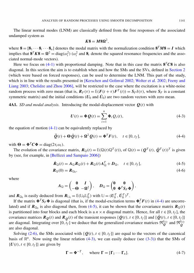
Figure 1 shows the relative errors between the canonical vectors e1 = (1, 0)T and e2 = (0, 1)T (theLNMs of (4-4)) and the approximations of these LNMs given by the SMs of the transient response{ Q(t), t 2 [0, t f ]} using (4-7), plotted versus the correlation coefficient ⇢ and for different values of t f

(t f = 0.1Tc, 0.2Tc, 0.5Tc, Tc, and 10Tc). First of all, in all the simulation results, the relative errors aresmall (less than 0.1) and, of course, the worse case corresponds to ⇢ = 1 and t f small. As expected, fora given t f , the relative error decreases as ⇢ decreases. When t f increases the SD coincides with the SDgiven by the stationary response (see the continuous line in Figure 1).

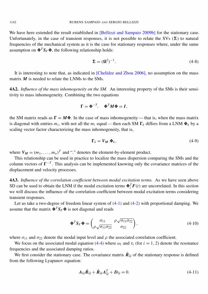
Under the same simulation conditions, Figure 2 shows the relative errors between the resonance fre-quencies !1 = 1 and !2 = 1.5 and the approximation of these resonance frequencies given by the SMs ofthe transient response { Q(t), t 2 [0, t f ]} using (4-8). Here also the relative errors are very small (less than0.001). Moreover, for fixed t f , the relative error does not depend on ⇢ and decreases when t f increases.

1144 RUBENS SAMPAIO AND SERGIO BELLIZZI

10!3

10!2

10!1

100

10!6

10!5

10!4

10!3

10!2

!

Rela

tive e

rror

e1

tf=0.1 T

c

tf=0.2 T

c

tf=0.5 T

c

tf=T

c

tf=10 T

c

!"#

!"#

!"#

"#

"#

Figure 1. Relative error (using Euclidean norm vector) between the canonical vector(e1 = (1, 0)T (left) and e2 = (0, 1)T (right)) and the approximation of these LNMs givenby the SMs of the transient response { Q(t), t 2 [0, t f ]} using (4-7) (dotted lines) and theapproximation of these LNMs given by the SMs of the stationary response (continuousline).

10!3

10!2

10!1

100

10!12

10!10

10!8

10!6

10!4

!

Re

lative

err

or

"1

tf=0.1 T

c

tf=0.2 T

c

tf=0.5 T

c

tf=T

c

tf=10 T

c

J

!"#$

!"#$

!"%#$

!#$

!#$

Figure 2. Relative error between the natural resonance-frequency vector (!1 (left) and!2 (right)) and the approximation of these LNMs given by the SMs of the transientresponse { Q(t), t 2 [0, t f ]} using (4-8) (dotted lines) and the approximation of theseLNMs given by the SMs of the stationary response (continuous line).

4B. Discrete nonlinear case. Consider a discrete mechanical system with n degrees of freedom. LetU(t) be the displacement vector at the instant t . We assume that U(t) satisfies the initial-value problem

MU(t) + H(U(t), U(t)) = F(t), t 2 [0, t f ] (4-17)

U(0) = U0, U(0) = U0, (4-18)

ANALYSIS OF RANDOM PROCESSES USING SMOOTH DECOMPOSITION 1145

where M is a symmetric square matrix with dimension n ⇥ n and H is a n-vector smooth nonlinearfunction. The vectors U0 and U0 define the initial conditions of the motion at t = 0, and {F(t), t 2 [0, t f ]}is a random vector process.

One rather interesting result was the difference between the SM obtained using the SD of the stationaryresponse of the nonlinear system and the SM obtained using the SD of the stationary response of theequivalent linear system obtained using statistical linearization, as described in [Kozin 1988].

Rewriting (4-17) as a nonlinear first-order differential equation (for U(t) = (U(t)T , U(t)T )T )

U(t) = N(U(t)) + G(t), (4-19)

with external random excitation G(t) = (0, (M�1 F(t))T )T . A suitable equivalent linear system can bewritten as

U(t) = LeqU(t) + G(t), (4-20)

where the constant matrix Leq is determined by

minL

E�kN(U(t)) � LU(t)k2�. (4-21)

Under the assumption that the nonlinear system (4-19) admits a stationary ergodic probability measure,it can be shown [Kozin 1988] that the stationary covariance matrix of the nonlinear response (4-19)coincides with the stationary covariance matrix of the equivalent linear response (4-20). Hence, theSD analysis of the stationary response of the nonlinear system (4-17) gives the same results as the SDanalysis of the stationary response of the equivalent linear system except for the SCs. Following themodal analysis described in the previous sections, the SD can also be viewed as a tool for modal analysisof the nonlinear system, the SMs and SVs of the nonlinear system being interpreted as in reference tothe modal characteristics of the linearized system.

5. Numerical example

We consider a finite chain of n mass points with the first one linked by a linear spring to a fixed point, theothers consecutively linked one to the other, and the last one linked only to the previous mass. All thestiffness coefficients of the strings are equal and their common value is 1. The mass values are denotedby mi (mi > 0). The system can also include isolated nonlinearities between consecutive masses of theform �i (Ui (t)�Ui�1(t))3 for i = 2, . . . , n. The associated equations of motion are of the form of (4-17),with

M =

0

BBBBBBB@

m1 0 0 · · · 0 00 m2 0 0 00 0 m3 0 0...

...

0 0 0 mn�1 00 0 0 · · · 0 mn

1

CCCCCCCA

, K =

0

BBBBBBB@

2 –1 0 · · · 0 0–1 2 –1 0 00 –1 2 0 0...

...

0 0 0 2 –10 0 0 · · · –1 1

1

CCCCCCCA

. (5-1)

H , which only depends on U(t), is easily deduced from the form of the nonlinearity. The dampingmatrix is chosen to be C = 2⌧1!1 M, with ⌧1 > 0, which assures that the damping is proportional and

1146 RUBENS SAMPAIO AND SERGIO BELLIZZI

fixes the damping ratio of the first linear mode. Note that the linear version of this system has beendiscussed in [Farooq and Feeny 2008].

Two excitation conditions will be considered:

• Uncorrelated excitation: the system is excited by a standard vector-valued white-noise process withmatrix intensity

SF = S0 M, (5-2)

with S0 > 0. This choice ensures that, for all mass values mi , 8T SF8 = S0 I is always diagonal.• Correlated excitation: the system is excited by a white-noise scalar process applied to the mass

numbered iexcit, that is,

F(t) = (0 · · · 010 · · · 0)T f (t) = P f (t), (5-3)

with { f (t), t 2 R} being a white-noise process with intensity S0 > 0. The intensity matrix of{F(t), t 2 R} is given by SF = S0 P PT and hence 8T SF8 = S0(8i iexcit8 j i ) is not a diagonal matrix.

The displacement and velocity histories were obtained from excitation histories by solving (4-17)over [0, t f ] numerically using the Newmark method. The excitation histories were simulated using theprocedure described in [Poirion and Soize 1989]. The following values of parameters were used: n = 10,m2 = 2, and mi = 1 for i 6= 2, ⌧1 = 0.05, �5 = 10, and �i = 0 for i 6= 5, S0 = 1, and for the correlatedcase, iexcit = 1. Zero initial displacement and velocity were assumed. The time-discretization parametervalue was chosen equal to 1t = 0.1 (that is, fe = 10) and 65536 instants were simulated. The last-halfpoints of the displacement and velocity histories were used to approximate the covariance matrices RUand RU of the stationary response. The simulated data were also used to estimate Leq solving (4-21)and the SDs of the stationary response of the equivalent linear system (4-20) were computed solving theassociated equation (4-11).

The estimated values of the resonance frequencies obtained from SD analysis are reported in Table 1.Note that the expression “resonance frequency” is a misnomer because the system is nonlinear; we will

Underlying Uncorrelated case Correlated caselinear system SD from: (4-17) (4-20) (4-17) (4-20)

!1 0.0236 0.0246 0.0246 0.0243 0.0243!2 0.0665 0.0705 0.0706 0.0696 0.0696!3 0.1068 0.1077 0.1074 0.1076 0.1073!4 0.1515 0.1656 0.1655 0.1626 0.1626!5 0.1960 0.1984 0.1983 0.1977 0.1978!6 0.2327 0.2430 0.2429 0.2418 0.2417!7 0.2491 0.2519 0.2521 0.2513 0.2514!8 0.2740 0.2862 0.2866 0.2850 0.2850!9 0.2980 0.3010 0.3013 0.2996 0.2997!10 0.3132 1.0234 1.0240 0.4533 0.4533

Table 1. Estimated values of the resonance frequencies obtained from SD analysis.

ANALYSIS OF RANDOM PROCESSES USING SMOOTH DECOMPOSITION 1147

use it in reference to the associated linearized system. As expected in the uncorrelated case, the estimatesobtained from the nonlinear system coincide with those given by the linearized system. These valuesare very close to the resonance-frequency values of the underlying linear system (that is, with �5 = 0)except for the last value which is larger due to the nonlinear term. The same comments hold also for thecorrelated case showing that the SD properties are robust to the loss of the noncorrelation assumption.Here also the numerical value of !10 is large, resulting in the effect of the nonlinear term which ishowever smaller than the uncorrelated case.

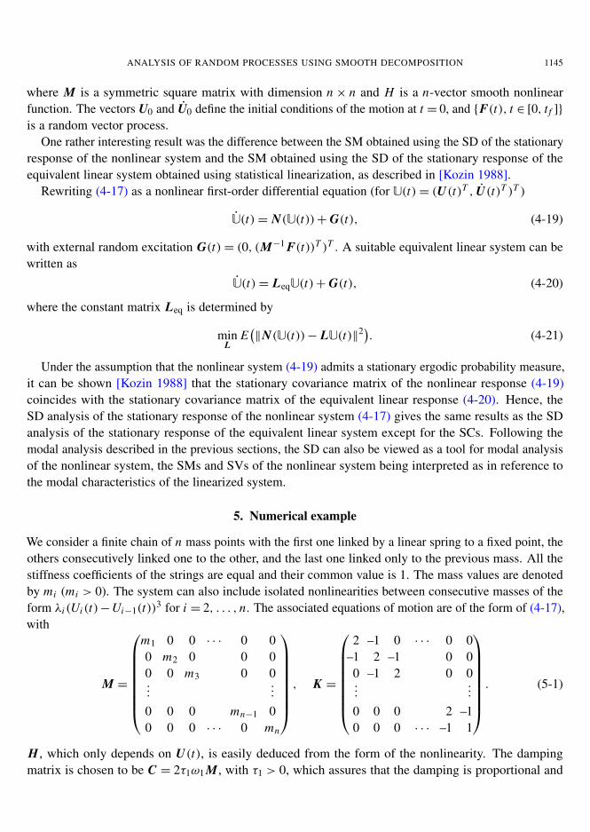
For the uncorrelated case, the SMs obtained from the stationary responses of the nonlinear system andthe linearized system are plotted in Figure 3. As expected in the uncorrelated case (see Section 4A1), theSMs obtained from the nonlinear system coincide with those given by the linearized system. The SMsdiffer significantly from the normal modes of the underlying linear system, also plotted in the figure. Forthe first modes, the difference occurs only around the mass number 2 where the mass inhomogeneity is

1 2 3 4 5 6 7 8 9 10

−0.4

−0.2

0(1)

1 2 3 4 5 6 7 8 9 10

−0.6

−0.4

−0.2

0

0.2

0.4(2)

1 2 3 4 5 6 7 8 9 10−0.4−0.2

00.20.40.60.8 (3)

1 2 3 4 5 6 7 8 9 10−0.4

−0.2

0

0.2

0.4 (4)

1 2 3 4 5 6 7 8 9 10−0.4

−0.2

0

0.2

0.4

0.6 (5)

1 2 3 4 5 6 7 8 9 10

−0.5

0

0.5

1 (6)

1 2 3 4 5 6 7 8 9 10

−0.6

−0.4

−0.2

0

0.2 (7)

1 2 3 4 5 6 7 8 9 10

−1

0

1(8)

1 2 3 4 5 6 7 8 9 10

−0.4

−0.2

0

0.2

0.4 (9)

mass number1 2 3 4 5 6 7 8 9 10

−50

0

50(10)

mass number

Figure 3. Uncorrelated case: the SMs (dashed lines and point markers) and the associ-ated normal modes given by 0�T (dotted-dashed lines and square markers), see (4-7),obtained from the nonlinear system. The normal modes of the underlying linear systemare also reported (dotted lines and circle markers).

1148 RUBENS SAMPAIO AND SERGIO BELLIZZI

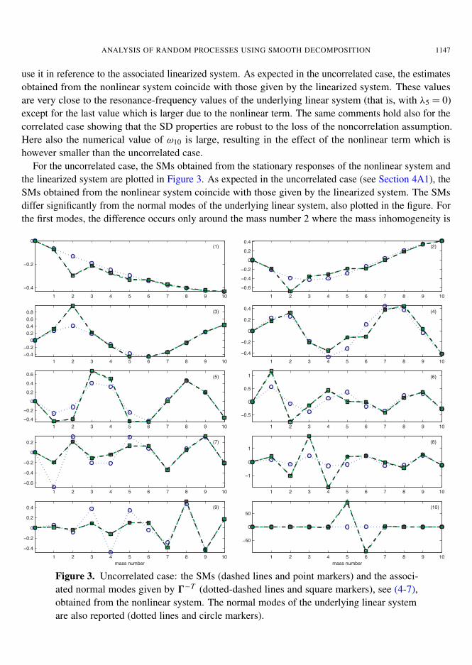
present. The relationship between the normal modes and the SMs is in line with (4-9). For the last mode(corresponding to !10), the difference between the normal mode and the SM occurs around the massnumbers 5 and 6, where there is local nonlinearity. At these two masses the amplitudes of the SMs arevery large and have opposite signs. The SMs, then, seem to be also sensitive to the nonlinearity of thesystem. In Figure 4, the modes obtained from the SMs of the stationary responses of the nonlinear systemand the linearized system are plotted and compared to the normal modes of the underlying linear system.The first modes are very similar. The difference increases for the middle and higher modes. For thecorrelated case, the SMs obtained from the stationary responses of the nonlinear system and the linearizedsystem are plotted in Figure 5 and compared to the normal modes of the underlying linear system. Forthe middle modes (vector 4 to vector 8), the nonlinear SMs differ from the linearized SMs. Here also,the SMs differ from the normal modes of the underlying linear system where the mass inhomogeneityis present (mass number 2) and where the local nonlinear term acts (mass numbers 5 and 6).

1 2 3 4 5 6 7 8 9 10

!0.4

!0.2

0(1)

1 2 3 4 5 6 7 8 9 10

!0.4

!0.2

0

0.2

0.4(2)

1 2 3 4 5 6 7 8 9 10

!0.4

!0.2

0

0.2

0.4 (3)

1 2 3 4 5 6 7 8 9 10

!0.4

!0.2

0

0.2

0.4(4)

1 2 3 4 5 6 7 8 9 10

!0.4

!0.2

0

0.2

0.4

0.6 (5)

1 2 3 4 5 6 7 8 9 10

0

0.5

1 (6)

1 2 3 4 5 6 7 8 9 10

!0.6

!0.4

!0.2

0

0.2 (7)

1 2 3 4 5 6 7 8 9 10

!1

0

1

(8)

1 2 3 4 5 6 7 8 9 10

!0.4

!0.2

0

0.2

0.4 (9)

mass number

1 2 3 4 5 6 7 8 9 10

!5

0

5 (10)

mass number

Figure 4. Uncorrelated case: the normal modes obtained from the nonlinear system(dashed lines and point markers), 0�T (see (4-7)), and form the linearized system(dotted-dashed lines and square markers). The normal modes of the underlying linearsystem are also reported (dotted lines and circle markers).

ANALYSIS OF RANDOM PROCESSES USING SMOOTH DECOMPOSITION 1149

1 2 3 4 5 6 7 8 9 10

!0.4

!0.2

0(1)

1 2 3 4 5 6 7 8 9 10

!0.6

!0.4

!0.2

0

0.2

0.4(2)

1 2 3 4 5 6 7 8 9 10

!0.4

!0.2

0

0.2

0.4

0.6

0.8 (3)

1 2 3 4 5 6 7 8 9 10

!0.4

!0.2

0

0.2

0.4(4)

1 2 3 4 5 6 7 8 9 10

!0.4

!0.2

0

0.2

0.4

0.6(5)

1 2 3 4 5 6 7 8 9 10

!0.5

0

0.5

1(6)

1 2 3 4 5 6 7 8 9 10

!0.6

!0.4

!0.2

0

0.2 (7)

1 2 3 4 5 6 7 8 9 10

!1

0

1 (8)

1 2 3 4 5 6 7 8 9 10

!0.4

!0.2

0

0.2

0.4 (9)

mass number

1 2 3 4 5 6 7 8 9 10

!2

0

2(10)

mass number

Figure 5. Correlated case: the SMs (dashed lines and point markers) and the associ-ated normal modes given by 0�T (dotted-dashed lines and square markers), see (4-7),obtained from the nonlinear system. The normal modes of the underlying linear systemare also reported (dotted lines and circle markers).

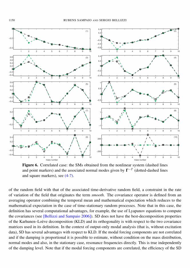
In Figure 6, the SMs of the stationary responses of the nonlinear system are compared to the modesobtained from the SMs of the stationary responses of the nonlinear system. Here also, the SMs differfrom the approximate normal modes where the mass inhomogeneity is present (mass number 2) andwhere the local nonlinear term acts (mass numbers 5 and 6). Note that these modes have been obtainedonly from data. This shows the ability of SD analysis to extract frequency, mode, and mass information.

6. Conclusions

In this paper, the smooth orthogonal decomposition method introduced in [Chelidze and Zhou 2006]was formulated in terms of a smooth decomposition (SD) (also called smooth Karhunen–Loève decom-position in [Bellizzi and Sampaio 2009b]) to analyze time-continuous nonstationary random processes.The SD is obtained by solving a generalized eigenproblem defined by combining the covariance matrix

1150 RUBENS SAMPAIO AND SERGIO BELLIZZI

1 2 3 4 5 6 7 8 9 10

!0.4

!0.2

0(1)

1 2 3 4 5 6 7 8 9 10

!0.6

!0.4

!0.2

0

0.2

0.4(2)

1 2 3 4 5 6 7 8 9 10

!0.4

!0.2

0

0.2

0.4

0.6

0.8 (3)

1 2 3 4 5 6 7 8 9 10!0.4

!0.2

0

0.2

0.4(4)

1 2 3 4 5 6 7 8 9 10

!0.4

!0.2

0

0.2

0.4

0.6(5)

1 2 3 4 5 6 7 8 9 10

!0.5

0

0.5

1(6)

1 2 3 4 5 6 7 8 9 10

!0.2

0

0.2(7)

1 2 3 4 5 6 7 8 9 10

!1

0

1(8)

1 2 3 4 5 6 7 8 9 10

!0.4

!0.2

0

0.2

0.4 (9)

mass number

1 2 3 4 5 6 7 8 9 10

!200

0

200(10)

mass number

Figure 6. Correlated case: the SMs obtained from the nonlinear system (dashed linesand point markers) and the associated normal modes given by 0�T (dotted-dashed linesand square markers), see (4-7).

of the random field with that of the associated time-derivative random field, a constraint in the rateof variation of the field that originates the term smooth. The covariance operator is defined from anaveraging operator combining the temporal mean and mathematical expectation which reduces to themathematical expectation in the case of time-stationary random processes. Note that in this case, thedefinition has several computational advantages, for example, the use of Lyapunov equations to computethe covariances (see [Bellizzi and Sampaio 2006]). SD does not have the best-decomposition propertiesof the Karhunen–Loève decomposition (KLD) and its orthogonality is with respect to the two covariancematrices used in its definition. In the context of output-only modal analysis (that is, without excitationdata), SD has several advantages with respect to KLD. If the modal forcing components are not correlatedand if the damping is proportional it is possible to estimate, without condition on the mass distribution,normal modes and also, in the stationary case, resonance frequencies directly. This is true independentlyof the damping level. Note that if the modal forcing components are correlated, the efficiency of the SD

ANALYSIS OF RANDOM PROCESSES USING SMOOTH DECOMPOSITION 1151

method to estimate resonance frequencies and normal modes rapidly decreases when the damping levelincreases. Beyond the modal analysis, another interesting property of the SD is that it is possible to extractthe mass distribution from the SD comparing the smooth modes (SMs) and the normal modes estimatedalso from the SMs. Finally, the SD can also be viewed as a tool for modal analysis of nonlinear systems.In the stationary case, the SMs and smooth values (SVs) of the nonlinear response coincide with the SMsand SVs of the response of the equivalent linear system obtained by a statistical linearization approach.Moreover under a constant mass matrix assumption, the SMs give access to the mass distribution.

References

[Bellizzi and Sampaio 2006] S. Bellizzi and R. Sampaio, “POMs analysis of randomly vibrating systems obtained fromKarhunen–Loève expansion”, J. Sound Vib. 297:3–5 (2006), 774–793.

[Bellizzi and Sampaio 2007] S. Bellizzi and R. Sampaio, “Analysis of randomly vibrating systems using Karhunen–Loève ex-pansion”, pp. 1387–1395 in Proceedings of the ASME International Design Engineering Technical Conferences & Computersand Information in Engineering Conference (Las Vegas, NV, 2007), vol. 1, ASME, New York, 2007. Paper #DETC2007-34431.

[Bellizzi and Sampaio 2009a] S. Bellizzi and R. Sampaio, “Karhunen–Loève modes obtained from displacement and velocityfields: assessments and comparisons”, Mech. Syst. Signal Process. 23:4 (2009), 1218–1222.

[Bellizzi and Sampaio 2009b] S. Bellizzi and R. Sampaio, “Smooth Karhunen–Loève decomposition to analyze randomlyvibrating systems”, J. Sound Vib. 325:3 (2009), 491–498.

[Chelidze and Zhou 2006] D. Chelidze and W. Zhou, “Smooth orthogonal decomposition-based vibration mode identification”,J. Sound Vib. 292:3–5 (2006), 461–473.

[Farooq and Feeny 2008] U. Farooq and B. F. Feeny, “Smooth orthogonal decomposition for modal analysis of randomlyexcited systems”, J. Sound Vib. 316:1–5 (2008), 137–146.

[Feeny and Liang 2003] B. F. Feeny and Y. Liang, “Interpreting proper orthogonal modes of randomly excited vibration sys-tems”, J. Sound Vib. 265:5 (2003), 953–966.

[Holmes et al. 1996] P. Holmes, J. L. Lumley, and G. Berkooz, Turbulence, coherent structures, dynamical systems and sym-metry, Cambridge University Press, Cambridge, 1996.

[Kerschen and Golinval 2002] G. Kerschen and J.-C. Golinval, “Physical interpretation of the proper orthogonal modes usingthe singular value decomposition”, J. Sound Vib. 249:5 (2002), 849–865.

[Kerschen et al. 2005] G. Kerschen, J.-C. Golinval, A. F. Vakakis, and L. A. Bergman, “The method of proper orthogonaldecomposition for dynamical characterization and order reduction of mechanical systems: an overview”, Nonlinear Dyn.41:1-3 (2005), 147–169.

[Kozin 1988] F. Kozin, “The method of statistical linearization for nonlinear stochastic vibrations”, pp. 45–56 in Nonlinearstochastic dynamic engineering systems (IUTAM Symposium) (Innsbruck, 1987), edited by F. Ziegler and G. I. Schuëller,Springer, Berlin, 1988.

[Lin et al. 2002] W. Z. Lin, K. H. Lee, P. Lu, S. P. Lim, and Y. C. Liang, “The relationship between eigenfunctions of Karhunen–Loève decomposition and the modes of distributed parameter vibration system”, J. Sound Vib. 256:4 (2002), 791–799.

[Poirion and Soize 1989] F. Poirion and C. Soize, “Simulation numérique des champs stochastiques Gaussiens homogènes etnon homogènes”, Rech. Aérosp. 1 (1989), 41–61.

[Quaranta et al. 2008] G. Quaranta, P. Masarati, and P. Mantegazza, “Continuous-time covariance approaches for modal analy-sis”, J. Sound Vib. 310:1–2 (2008), 287–312.

[Wolter et al. 2002] C. Wolter, M. A. Trindade, and R. Sampaio, “Obtaining mode shapes through the Karhunen–Loève expan-sion for distributed-parameter linear systems”, Shock Vib. 9:4–5 (2002), 177–192.

[Zhou 2006] W. Zhou, Multivariate analysis in vibration modal parameter identification, Ph.D. thesis, University of RhodeIsland, 2006, Available at http://gradworks.umi.com/32/48/3248248.html.

1152 RUBENS SAMPAIO AND SERGIO BELLIZZI

Received 20 May 2010. Revised 27 Sep 2010. Accepted 14 Nov 2010.

RUBENS SAMPAIO: rsampaio@puc-rio.br

Departamento de Engenharia Mecânica, PUC-Rio, Rua Marquês de São Vicente, 225, 22453-900 Rio de Janeiro-RJ, Brazil

SERGIO BELLIZZI: bellizzi@lma.cnrs-mrs.fr

Laboratoire de Mécanique et d’Acoustique - CNRS, 31 chemin Joseph Aiguier, 13402 Marseille, France

mathematical sciences publishers msp

JOURNAL OF MECHANICS OF MATERIALS AND STRUCTURESjomms.org

Founded by Charles R. Steele and Marie-Louise Steele

EDITORS

CHARLES R. STEELE Stanford University, USADAVIDE BIGONI University of Trento, ItalyIWONA JASIUK University of Illinois at Urbana-Champaign, USA

YASUHIDE SHINDO Tohoku University, Japan

EDITORIAL BOARD

H. D. BUI École Polytechnique, FranceJ. P. CARTER University of Sydney, Australia

R. M. CHRISTENSEN Stanford University, USAG. M. L. GLADWELL University of Waterloo, Canada

D. H. HODGES Georgia Institute of Technology, USAJ. HUTCHINSON Harvard University, USA

C. HWU National Cheng Kung University, TaiwanB. L. KARIHALOO University of Wales, UK

Y. Y. KIM Seoul National University, Republic of KoreaZ. MROZ Academy of Science, Poland

D. PAMPLONA Universidade Católica do Rio de Janeiro, BrazilM. B. RUBIN Technion, Haifa, Israel

A. N. SHUPIKOV Ukrainian Academy of Sciences, UkraineT. TARNAI University Budapest, Hungary

F. Y. M. WAN University of California, Irvine, USAP. WRIGGERS Universität Hannover, Germany

W. YANG Tsinghua University, ChinaF. ZIEGLER Technische Universität Wien, Austria

PRODUCTION contact@msp.org

SILVIO LEVY Scientific Editor

Cover design: Alex Scorpan Cover photo: Mando Gomez, www.mandolux.com

See http://jomms.org for submission guidelines.

JoMMS (ISSN 1559-3959) is published in 10 issues a year. The subscription price for 2011 is US $520/year for the electronicversion, and $690/year (+$60 shipping outside the US) for print and electronic. Subscriptions, requests for back issues, and changesof address should be sent to Mathematical Sciences Publishers, Department of Mathematics, University of California, Berkeley,CA 94720–3840.

JoMMS peer-review and production is managed by EditFLOW™ from Mathematical Sciences Publishers.

PUBLISHED BYmathematical sciences publishers

http://msp.org/A NON-PROFIT CORPORATION

Typeset in LATEXCopyright ©2011 by Mathematical Sciences Publishers

Journal of Mechanics of Materials and StructuresVolume 6, No. 7-8September–October 2011

Special issueEleventh Pan-American Congress

of Applied Mechanics (PACAM XI)

Preface ADAIR R. AGUIAR 949

Influence of specimen geometry on the Portevin–Le Châtelier effect due to dynamic strain agingfor the AA5083-H116 aluminum alloy

RODRIGO NOGUEIRA DE CODES and AHMED BENALLAL 951

Dispersion relations for SH waves on a magnetoelectroelastic heterostructure with imperfectinterfacesJ. A. OTERO, H. CALAS, R. RODRÍGUEZ, J. BRAVO, A. R. AGUIAR and G. MONSIVAIS 969

Numerical linear stability analysis of a thermocapillary-driven liquid bridge with magneticstabilization YUE HUANG and BRENT C. HOUCHENS 995

Numerical investigation of director orientation and flow of nematic liquid crystals in a planar 1:4expansion PEDRO A. CRUZ, MURILO F. TOMÉ, IAIN W. STEWART and SEAN MCKEE 1017

Critical threshold and underlying dynamical phenomena in pedestrian-induced lateralvibrations of footbridges STEFANO LENCI and LAURA MARCHEGGIANI 1031

Free vibration of a simulation CANDU nuclear fuel bundle structure inside a tubeXUAN ZHANG and SHUDONG YU 1053

Nonlinear dynamics and sensitivity to imperfections in Augusti’s modelD. ORLANDO, P. B. GONÇALVES, G. REGA and S. LENCI 1065

Active control of vortex-induced vibrations in offshore catenary risers: A nonlinear normal modeapproach CARLOS E. N. MAZZILLI and CÉSAR T. SANCHES 1079

Nonlinear electromechanical fields and localized polarization switching of piezoelectricmacrofiber composites

YASUHIDE SHINDO, FUMIO NARITA, KOJI SATO and TOMO TAKEDA 1089

Three-dimensional BEM analysis to assess delamination cracks between two transverselyisotropic materials

NICOLÁS O. LARROSA, JHONNY E. ORTIZ and ADRIÁN P. CISILINO 1103

Porcine dermis in uniaxial cyclic loading: Sample preparation, experimental results andmodeling A. E. EHRET, M. HOLLENSTEIN, E. MAZZA and M. ITSKOV 1125

Analysis of nonstationary random processes using smooth decompositionRUBENS SAMPAIO and SERGIO BELLIZZI 1137

Perturbation stochastic finite element-based homogenization of polycrystalline materialsS. LEPAGE, F. V. STUMP, I. H. KIM and P. H. GEUBELLE 1153

A collocation approach for spatial discretization of stochastic peridynamic modeling of fractureGEORGIOS I. EVANGELATOS and POL D. SPANOS 1171

JournalofMechanics

ofMaterials

andStructures

2011V

ol.6,No.7-8