Global decomposition experiment shows soil animalimpacts on decomposition are climate-dependent

D I A N A H . WA L L *, M A R K A . B R A D F O R D w , M A R K G . S T . J O H N z, J O H N A . T R O F Y M O W § ,

VA L E R I E B E H A N - P E L L E T I E R } , D AV I D E . B I G N E L L k, J . M A R K D A N G E R F I E L D **,

W I L L I A M J . PA R T O N w w, J O S E F R U S E K zz, W I N F R I E D V O I G T § § , V O L K M A R W O L T E R S } } ,

H O L L E Y Z A D E H G A R D E L w w, F R E D O . AY U K E kk, R I C H A R D B A S H F O R D ***,

O L G A I . B E L J A K O VA w w w, PA T R I C K J . B O H L E N zzz, A L A I N B R A U M A N § § § ,

S T E P H E N F L E M M I N G } } }, J O H R . H E N S C H E L kkk, D A N L . J O H N S O N ****,

T . H E F I N J O N E S w w w w , M A R C E L A K O VA R O VA zzzz, J . M A R T Y K R A N A B E T T E R § § § § ,

L E S K U T N Y } } } } , K U O - C H U A N L I N kkkk, M O H A M E D M A R YA T I *****,

D O M I N I Q U E M A S S E w w w w w, A N D R E I P O K A R Z H E V S K I I zzzzz{,

H O M AT H E V I R A H M A N *****, M I L L O R G . S A B A R A § § § § §, J O E R G - A L F R E D S A L A M O N } } ,

M I C H A E L J . S W I F T } } } } } , A M A N D A VA R E L A kkkkk, H E R A L D O L . VA S C O N C E L O S ******,

D O N W H I T E w w w w w w and X I A O M I N G Z O U zzzzzz§ § § § § §

*Natural Resource Ecology Laboratory and Department of Biology, Colorado State University, Fort Collins, CO 80523, USA,

wOdum School of Ecology, University of Georgia, Athens, GA 30602, USA, zLandcare Research, PO Box 40, Lincoln 7640, New

Zealand, §Canadian Forest Service, Pacific Forestry Centre, Victoria, BC, Canada V8Z 1M5, }Agriculture and Agri-food Canada,

Ottawa, ON, Canada K1A 0C6, kQueen Mary University of London, London E1 4NS, UK, **Macquarie University, Sydney, NSW

2109, Australia, wwNatural Resource Ecology Laboratory, Colorado State University, Fort Collins, CO 80523, USA, zzInstitute of

Soil Biology, Academy of Sciences, Ceske Budejovice 370 05, Czech Republic, §§Institute of Ecology, University of Jena, Jena 07743,

Germany, }}Department of Animal Ecology, Justus-Liebig-University, D-35392 Giessen, Germany, kkKenya Methodist University,

Kaaga Campus, Meru, Kenya, ***Forest Entomology, Forestry Tasmania, Hobart, TAS 7000, Australia, wwwCentralno-

Chernozemnyj Reserve, Zapovednoe, Russian Federation, zzzMacArthur Agro-Ecology Research Center, Lake Placid, FL 33852,

USA, §§§Laboratoire MOST Centre IRD, Institut de Recherche pour le Developpement, UR SeqBio, SupAgro, Montpellier, France,

}}}Gros Morne National Park, Rocky Harbour, NL, Canada A0K 4N0, kkkGobabeb Training & Research Centre, Box 953, Walvis

Bay, Namibia, ****Department of Geography, University of Lethbridge, Lethbridge, AB, Canada T1K 3M4, wwwwCardiff School of

Biosciences, Cardiff University, Cardiff CF10 3US, UK, zzzzInstitute of Botany, Academy of Sciences, Pruhonice 252 43, Czech

Republic, §§§§B.C. Ministry of Forests, Smithers, BC, Canada V0J 2N0, }}}}Inuvik Research Centre, Inuvik, NT, Canada X0E

0T0, kkkkTaiwan Forestry Research Institute, Taipei 100, Taiwan, *****Institute of Tropical Biology and Conservation, Universiti

Malaysia Sabah, Sabah, Malaysia, wwwwwInstitut de Recherche pour le Developpement, Ouagadougou 01 BP182, Burkina Faso,

zzzzzInstitute of Ecology and Evolution of RAS, Moscow 119071, Russian Federation, §§§§§Centro Universitario do Leste de Minas

Gerais, Coronel Fabriciano 35170-056, Brazil, }}}}}Tropical Soil Biology & Fertility Institute of CIAT, ICRAF, Nairobi, Kenya,

kkkkkPontificia Universidad Javeriana, Bogota, DC, Colombia, ******Institute of Biology, Federal University of Uberlandia, CP 593,

38400-902 Uberlandia, Brazil, wwwwwwForest Resources, Department of Indian and Northern Affairs, Whitehorse, YT, Canada Y1A

2B5, zzzzzzXishuangbanna Tropical Botanical Garden, The Chinese Academy of Sciences, Kunming, Yunnan 650223, China,

§§§§§§Institute for Tropical Ecosystem Studies, University of Puerto Rico, San Juan 00931-1910, Puerto Rico

OnlineOpen: This article is available free online at www.blackwell-synergy.com

Abstract

Climate and litter quality are primary drivers of terrestrial decomposition and, based on

evidence from multisite experiments at regional and global scales, are universally

factored into global decomposition models. In contrast, soil animals are considered

key regulators of decomposition at local scales but their role at larger scales is

unresolved. Soil animals are consequently excluded from global models of organic

mineralization processes. Incomplete assessment of the roles of soil animals stems from

Correspondence: Diana H. Wall, tel. 1 1 970 491 2504, fax 1 1 970

491 1965, e-mail: Diana@nrel.colostate.edu

{Deceased.

Global Change Biology (2008) 14, 2661–2677, doi: 10.1111/j.1365-2486.2008.01672.x

r 2008 The AuthorsJournal compilation r 2008 Blackwell Publishing Ltd 2661

the difficulties of manipulating invertebrate animals experimentally across large geo-

graphic gradients. This is compounded by deficient or inconsistent taxonomy. We report

a global decomposition experiment to assess the importance of soil animals in C

mineralization, in which a common grass litter substrate was exposed to natural

decomposition in either control or reduced animal treatments across 30 sites distributed

from 431S to 681N on six continents. Animals in the mesofaunal size range were

recovered from the litter by Tullgren extraction and identified to common specifications,

mostly at the ordinal level. The design of the trials enabled faunal contribution to be

evaluated against abiotic parameters between sites. Soil animals increase decomposition

rates in temperate and wet tropical climates, but have neutral effects where temperature

or moisture constrain biological activity. Our findings highlight that faunal influences on

decomposition are dependent on prevailing climatic conditions. We conclude that (1)

inclusion of soil animals will improve the predictive capabilities of region- or biome-

scale decomposition models, (2) soil animal influences on decomposition are important at

the regional scale when attempting to predict global change scenarios, and (3) the

statistical relationship between decomposition rates and climate, at the global scale, is

robust against changes in soil faunal abundance and diversity.

Keywords: climate decomposition index, decomposition, litter, mesofauna, soil biodiversity, soil

carbon, soil fauna

Received 28 February 2008 and accepted 18 April 2008

Introduction

The annual global release of carbon to the atmosphere

through decomposition of organic carbon by soil biota is

approximately 50–75 Pg, nearly 10 times that of fossil fuel

emissions (Schimel et al., 1996). Climate and plant litter

quality (i.e. chemical composition) are considered the

primary regulators of litter decomposition, explaining as

much as 65–77% of the variation in decomposition rates

(Moorhead et al., 1999; Gholz et al., 2000; Trofymow et al.,

2002). The residual variation (ca. 25%) in global decom-

position rate models remains a substantial source of error

in estimates of contemporary and future global carbon

dynamics (Schimel et al., 1996; Del Grosso et al., 2005).

Putatively, the unallocated error in global decomposi-

tion models has a significant biological component, for

example organismal biomass, size distribution, taxo-

nomic richness, and/or functional group composition.

These components are normally considered as either

the direct effects of physical conditions (through addi-

tion or removal of habitats and therefore species) or

indirect effects (delivered via multiple climate effects

defining plant communities and the area of distribution

available to major groups of soil organisms). Conse-

quently, biota (animals and microbes) are not explicitly

considered in global decomposition models (VEMAP,

1995; Moorhead et al., 1999; Gholz et al., 2000; Lavelle

et al., 2004), although conceptually considered to be key

drivers of litter decomposition rates (e.g. Wardle, 1995;

Lavelle, 1997; Coleman & Hendrix, 2000; Kibblewhite

et al., 2008). Instead, soil biota have been evaluated

(relative to nonbiotic agencies) for their contribution

to aggregated ecosystem functions (or services, sensu

Daily et al., 1997; Wall, 2004), including decomposition,

together with the related processes of carbon sequestra-

tion and greenhouse gas emission. To refine this con-

cept, ecosystem services have been apportioned to

functional assemblages of named organisms (for exam-

ple Lavelle, 1997; Swift et al., 2004; Kibblewhite et al.,

2008), such that the effects of specific disturbances on

the delivery of individual services can be elucidated

(Wardle, 2002). The modeling, however, is at best semi-

quantitative and, most crucially, it is ecosystem-specific

and cannot be deployed much beyond the landscape

scale or made responsive to the incremental changes in

physical environmental parameters inherent in climate

change scenarios. To factor soil biota into future global

decomposition modeling, it is necessary to assess de-

composition against a biotic assemblage character on a

supraregional scale and by an experimental procedure

that will adequately distinguish between the abiotic and

the biotic agencies responsible for the process.

Almost 30 years ago, Swift et al. (1979) hypothesized

that the relative contribution of soil fauna (vs. micro-

flora) to decomposition was dependent on the climatic

region, being greatest at midlatitudes and decreasing

towards the poles. In contrast to the many multisite

experiments on climate and litter quality (Moorhead

et al., 1999; Trofymow et al., 2002), relationships between

soil animals and litter decomposition have never been

experimentally tested at global or regional scales.

Furthermore, there are few data to judge the signifi-

cance of changes in diversity of soil fauna at these scales

(Swift et al., 1998), which reflects the scarcity of the

2662 D . H . WA L L et al.

r 2008 The AuthorsJournal compilation r 2008 Blackwell Publishing Ltd, Global Change Biology, 14, 2661–2677

required taxonomic expertize and the prohibitive effort

needed to characterize biota in a sufficient number of

sites and with a resolution that reflects true biodiversity.

Inferences from local scale and the few cross-site ex-

periments that manipulated animals (Heneghan et al.,

1999; Gonzalez & Seastedt, 2001) are restricted by the

low number of sites, differences in litter types and

qualities between experiments, and the fact that due

to a vast and mostly unknown biodiversity in many

biomes, invertebrate analyses have been typically

restricted to one to three taxonomic groups.

The Global Litter Invertebrate Decomposition Experi-

ment (GLIDE) tests the hypothesis that soil animals

significantly influence litter decomposition rates, over

and above climate alone, at regional and global scales.

A second hypothesis, related to the first and following

Swift et al. (1979), is that the role of animals in terrestrial

decomposition changes from region to region rather

than having a single global character. The centerpiece

of GLIDE’s design was the use of a single plant litter

substrate, of known quality and from a single origin,

which was exposed in standard litterbags while manip-

ulating the abundance and richness of soil fauna with a

generalized suppressor (naphthalene). Decomposition

was monitored in both animal-suppressed bags and

untreated controls by gravimetric measurement and

chemical analysis at 30 sites distributed across broad

climatic regions from 431S to 681N (Table 1). Addition-

ally, the extraction and characterization of associated

(mainly mesofaunal) invertebrate animals was assessed.

The use of the faunal-suppressant separated climate

from animal effects on litter decomposition. Animal data,

with complementary information on local climate and

the weight and carbon content of litter at the start of the

decomposition process and after exposure in the field,

show that soil animals positively influence decomposi-

tion rates in the temperate and wet tropical biomes.

Material and methods

Site management and location

Forty-one sites were initially established in 2001–02, as

part of the DIVERSITAS IBOY (International Biodiver-

sity Year) Project network, and with ILTER (Interna-

tional Long Term Ecological Research) collaborators.

Sites were selected to achieve the fullest practical climatic

and geographic range, but partially reflected the mostly

volunteer participation by national science teams in IBOY.

Eleven sites were dropped from analyses due to destruc-

tion of bags in situ, excessive extraneous organic matter or

soil in the litterbags, or where export of specimens from

countries was prohibited or impractical. The 30 remaining

sites are described in Table 1.

Experimental design

Two thousand glass-fiber, 20 cm� 20 cm, 2 mm mesh

litterbags (Harmon et al., 1999), were each filled with

10 � 0.5 g dried, gamma-sterilized grass hay [Agropyron

cristatum (L.) Gaertn.] foliar litter that had been air-

dried for 2 years at o20% rH. The litter, with all florets

removed, was preprocessed through a 1.0 mm screen (to

remove loose material before shipping) and then

shipped from Colorado State University (CSU) in the

constructed glass-fiber bags to sites. A single litter

quality was selected to facilitate site-to-site comparisons

and because the scale of resources required to analyze

all taxa from just one litter type made multilitter field

experiments unfeasible. Bags were weighed on-site to the

nearest 0.001 g before being secured to the soil surface,

and then progressively removed over time intervals. Of

24 bags at each site, six were placed randomly in each of

four experimental blocks. Within each block, three bags

were spaced along each of two paired 20 m transects,

with each transect being assigned to either the control or

animal-suppressed treatment. Transects ran parallel to

each other and were 10 m apart. The three bags within

each transect were spaced at 0, 10, and 20 m. All blocks

were at least 10 m apart, and positioned randomly. This

design was chosen to (a) ensure the suppression treat-

ment did not influence the control litterbags, (b) reduce

the impacts of disturbance by vertebrates, and (c) reduce

the effects of spatial autocorrelation.

Naphthalene treatment: animal suppression

The animal inhibitor naphthalene was added to half of

the litterbags; the other half was assigned to untreated

controls. Naphthalene was applied at the start of the

experiment in crystalline form (as ‘mothballs’ from a

single commercial source) and again at each sampling

occasion to litterbags that remained in the field for later

retrieval. For each treatment renewal, two mothballs

(�33.17 g per mothball) were placed adjacent to treat-

ment bags. Naphthalene was chosen to displace soil

animals because it reportedly has less biocidal effects

than other pesticides (Blair et al., 1989). An additional

three ‘traveler bags’ were shipped to each site, placed in

the field, immediately retrieved, reweighed, and re-

shipped to CSU for analysis. Traveler bags controlled

for material loss due to handling (Harmon et al., 1999).

See also www.nrel.colostate.edu/projects/glide/study

design.html.

Litterbag retrieval and processing

One control and one treatment litterbag were retrieved

from each block on three sampling occasions. Time of

S O I L FA U N A I M PA C T S O N G L O B A L D E C O M P O S I T I O N 2663

r 2008 The AuthorsJournal compilation r 2008 Blackwell Publishing Ltd, Global Change Biology, 14, 2661–2677

Tab

le1

GL

IDE

site

des

crip

tio

ns,

GL

IDE

clim

atic

reg

ion

s,an

dan

nu

alC

DI

val

ues

Co

un

try

Sit

e

cod

e

Lat

itu

de

Lo

ng

itu

de

So

ilty

pe

Veg

etat

ion

typ

eH

old

rid

ge

Lif

eZ

on

e

GL

IDE

clim

ate

reg

ion

Pre

cip

itat

ion

(cm

)

Tem

per

atu

re

(1C

)

An

nu

al

CD

I

Au

stra

lia

TA

S1

431040 S

1461

400 E

Pla

no

sol

Cal

lid

end

rou

sfe

rnra

info

rest

Co

ol

tem

per

ate

mo

ist

fore

stT

emp

erat

e11

0.1

8.8

0.27

11

Au

stra

lia

TA

S2

431040 S

1461

400 E

Acr

iso

lIn

term

edia

tera

info

rest

Co

ol

tem

per

ate

mo

ist

fore

stT

emp

erat

e11

0.1

8.8

0.27

11

Bra

zil

MA

N02

1250 S

601000 W

Fer

rals

ol

Tro

pic

alm

ois

tfo

rest

Tro

pic

alra

info

rest

Wet

tro

pic

al21

1.1

26.3

0.83

11

Bra

zil

RU

B19

1300 S

421300 W

Fer

rals

ol,

Acr

iso

l

Tro

pic

alra

info

rest

Su

btr

op

ical

rain

fore

stW

ettr

op

ical

116.

822

.70.

4881

Bu

rkin

aF

aso

BO

N111200 N

41150 W

Lu

vis

ol

Sh

rub

tow

oo

ded

sav

ann

aT

rop

ical

dry

fore

stD

rytr

op

ical

95.7

27.1

0.41

50

Can

ada

INU

681190 N

1331

320 W

Gle

yso

lB

lack

spru

ce,

pap

erb

irch

fore

stS

ub

po

lar

dry

tun

dra

Co

ldo

rd

ry17

.3�

11.3

0.04

43

Can

ada

YU

K60

1510 N

1351

120 W

Lu

vis

ol

Pin

e,sp

ruce

,as

pen

fore

stB

ore

alm

ois

tfo

rest

Co

ldo

rd

ry26

.5�

4.2

0.05

83

Can

ada

TO

P54

1360 N

1261

180 W

Lu

vis

ol

Pin

e,b

alsa

m,

fir,

spru

cefo

rest

Co

ol

tem

per

ate

mo

ist

fore

stC

old

or

dry

48.8

2.1

0.10

71

Can

ada

LE

T50

1110 N

1131

540 W

Ch

ern

oze

mF

escu

eg

rass

lan

dC

oo

lte

mp

erat

est

epp

eC

old

or

dry

44.3

4.4

0.14

77

Can

ada

VA

N48

1380 N

1231

420 W

Cam

bis

ol

Do

ug

las

fir

fore

stC

oo

lte

mp

erat

ew

etfo

rest

Tem

per

ate

196.

06.

20.

2287

Can

ada

RO

C49

1320 N

581490 W

Po

dzo

lB

alsa

mfi

r,w

hit

eb

irch

fore

stB

ore

alw

etfo

rest

Tem

per

ate

115.

21.

60.

2287

Can

ada

ON

E49

1010 N

1101

230 W

Ch

ern

oze

mS

ho

rtg

rass

Co

ol

tem

per

ate

step

pe

Co

ldo

rd

ry36

.03.

90.

1080

Ch

ina

XIS

211410 N

1011

250 E

Acr

iso

lT

rop

ical

seas

on

alra

info

rest

Su

btr

op

ical

mo

ist

fore

stW

ettr

op

ical

132.

220

.50.

5275

Co

lom

bia

BO

G04

1370 N

741180 W

An

do

sol,

Cam

bis

ol

Mo

nta

ne

clo

ud

fore

stT

rop

ical

wet

fore

stD

rytr

op

ical

117.

514

.70.

4288

Cze

chR

ep.

BIO

481420 N

161490 E

Flu

vis

ol

Rip

aria

no

akfo

rest

Co

ol

tem

per

ate

mo

ist

fore

stT

emp

erat

e54

.09.

30.

2462

Cze

chR

ep.

SU

M49

1970 N

131450 E

Cam

bis

ol

Mo

un

tain

clim

axsp

ruce

fore

stC

oo

lte

mp

erat

em

ois

tfo

rest

Tem

per

ate

64.8

7.6

0.25

37

Cze

chR

ep.

KO

M48

1420 N

161490 E

Flu

vis

ol

Rip

aria

no

akfo

rest

Co

ol

tem

per

ate

mo

ist

fore

stT

emp

erat

e54

.09.

30.

2462

Cze

chR

ep.

PA

L48

1420 N

161490 E

Ren

dzi

na

Xer

oth

erm

icg

rass

/d

ecid

uo

us

fore

stC

oo

lte

mp

erat

est

epp

eT

emp

erat

e54

.09.

30.

2462

2664 D . H . WA L L et al.

r 2008 The AuthorsJournal compilation r 2008 Blackwell Publishing Ltd, Global Change Biology, 14, 2661–2677

Ger

man

yG

IE51

1200 N

101220 E

Lu

vis

ol

Tem

per

ate

bee

chfo

rest

Co

ol

tem

per

ate

mo

ist

fore

stT

emp

erat

e68

.38.

10.

2618

Ger

man

yJE

N50

1570 N

111350 E

Ren

dzi

na

Xer

oth

erm

icg

rass

lan

dC

oo

lte

mp

erat

est

epp

eT

emp

erat

e58

.68.

20.

2432

Ken

ya

KE

N01

150 S

341500 E

Acr

iso

lR

ain

fore

stT

rop

ical

wet

fore

stW

ettr

op

ical

185.

620

.70.

6406

Mal

aysi

aM

AL

051470 N

1161

240 E

Acr

iso

lT

rop

ical

low

erm

on

tan

efo

rest

Su

btr

op

ical

wet

fore

stW

ettr

op

ical

260.

722

.80.

7587

Nam

ibia

NA

M23

1330 S

151020 E

Gle

yso

l,

His

toso

l

Sp

arse

dw

arf

shru

bS

ub

tro

pic

ald

eser

tC

old

or

dry

0.1

23.5

0.02

64

Ru

ssia

KU

R51

1340 N

361050 E

Ch

ern

oze

mO

akfo

rest

,m

ead

ow

step

pe

Co

ol

tem

per

ate

step

pe

Tem

per

ate

65.2

5.5

0.22

53

Sen

egal

SE

N16

1250 N

151300 W

Are

no

sol

Dry

sav

ann

a,b

alan

ites

Tro

pic

ald

eser

tsc

rub

Dry

tro

pic

al26

.127

.10.

1565

Tai

wan

TA

I24

1460 N

1211

350 E

Acr

iso

l,

Cam

bis

ol

Ev

erg

reen

,h

ard

wo

od

fore

stS

ub

tro

pic

alm

ois

tfo

rest

Wet

tro

pic

al20

8.2

20.6

0.73

13

UK

CA

R51

1500 N

041100 E

Cam

bis

ol

Oak

fore

stC

oo

lte

mp

erat

em

ois

tfo

rest

Tem

per

ate

82.6

9.8

0.29

61

UK

SIL

511240 N

01400 W

Cam

bis

ol

Oak

,o

ak-b

irch

,al

der

fore

stC

oo

lte

mp

erat

em

ois

tfo

rest

Tem

per

ate

74.1

9.3

0.24

14

US

AC

OL

401490 N

1041

460 W

Yer

mo

sol

Sh

ort

gra

ssst

epp

eC

oo

lte

mp

erat

est

epp

eC

old

or

dry

38.5

8.7

0.12

22

US

AF

LO

271090 N

811120 W

Lu

vis

ol,

His

toso

l

Nat

ive

tall

gra

ssw

etp

rair

ieS

ub

tro

pic

alm

ois

tfo

rest

Wet

tro

pic

al12

7.4

22.7

0.60

60

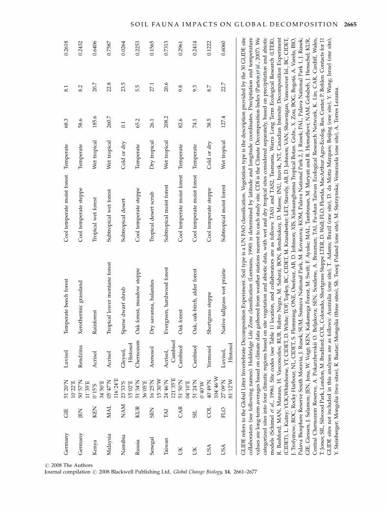
GL

IDE

refe

rsto

the

Glo

bal

Lit

ter

Inv

erte

bra

teD

eco

mp

osi

tio

nE

xp

erim

ent.

So

ilty

pe

isa

UN

FAO

clas

sifi

cati

on

.V

eget

atio

nty

pe

isth

ed

escr

ipti

on

pro

vid

edb

yth

e30

GL

IDE

site

coll

abo

rato

rs(s

eefo

llo

win

gn

ames

).H

old

rid

ge

Lif

eZ

on

ecl

assi

fica

tio

n(L

eem

ans,

1990

)is

det

erm

ined

by

lati

tud

ean

dlo

ng

itu

de

coo

rdin

ates

.P

reci

pit

atio

nan

dte

mp

erat

ure

val

ues

are

lon

g-t

erm

aver

ages

bas

edo

ncl

imat

ed

ata

gat

her

edfr

om

wea

ther

stat

ion

sn

eare

stto

each

stu

dy

site

.C

DI

isth

eC

lim

ate

Dec

om

po

siti

on

Ind

ex(P

arto

net

al.,

2007

).W

e

cate

go

rize

dsi

tes

into

fou

rcl

imat

icre

gio

ns

bas

edo

nsi

tev

eget

atio

nan

dab

ioti

cd

ata,

wit

hw

etan

dd

rytr

op

ical

site

sco

nsi

der

edse

par

atel

y,b

ased

on

pre

cip

itat

ion

and

abio

tic

mo

del

s(S

chim

elet

al.,

1996

).S

ite

cod

es(s

eeT

able

1)lo

cati

on

,an

dco

llab

ora

tors

are

asfo

llo

ws:

TA

S1

and

TA

S2,

Tas

man

ia,

War

raL

on

gT

erm

Eco

log

ical

Res

earc

h(L

TE

R),

R.

Bas

hfo

rd;

MA

N,

Man

aus,

H.

Vas

con

celo

s;R

UB

,R

ub

roN

egra

,M

.S

abar

a;

BO

N,

Bo

nd

ou

ku

y,D

.M

asse

;IN

U,

Inu

vik

,N

T,

Can

adia

nIn

ters

ite

Dec

om

po

siti

on

Ex

per

imen

t

(CID

ET

),L

.Ku

tny

;Y

UK

,Wh

iteh

ors

e,Y

T,

CID

ET

,D

.W

hit

e;T

OP,

To

ple

y,B

C,

CID

ET

,M

.K

ran

abet

ter;

LE

T,S

tav

ely,

AB

,D

.Jo

hn

son

;V

AN

,S

haw

nig

an,

Van

cou

ver

Isl.

,B

C,

CID

ET

,

J.T

rofy

mo

w;

RO

C,

Ro

cky

Har

bo

ur,

NL

,C

IDE

T,

S.

Fle

mm

ing

;O

NE

,O

nef

ou

r,A

B,

D.

Joh

nso

n;

XIS

,X

ish

uan

gb

ann

aT

rop

ical

Bo

tan

.G

rdn

.,X

.Z

ou

;B

OG

,B

og

ota

,A

.V

arel

a;B

IO,

Pal

ava

Bio

sph

ere

Res

erv

eS

ou

thM

ora

via

,J.

Ru

sek

;S

UM

,S

um

ava

Nat

ion

alP

ark

,M

.K

ov

aro

va;

KO

M,

Pal

ava

Nat

ion

alP

ark

2,J.

Ru

sek

;P

AL

,P

alav

aN

atio

nal

Par

k1,

J.R

use

k;

GIE

,G

iess

en,

J.S

alam

on

;JE

N,

Jen

a,W

.V

oig

t;K

EN

,K

akam

ega

Fo

rest

,M

.S

wif

t;F.

Ay

uk

e;M

AL

,T

amb

un

an,

M.

Mar

yat

ian

dR

.H

om

ath

evi;

NA

M,

Go

bab

eb,

J.H

ensc

hel

;K

UR

,

Cen

tral

Ch

ern

oze

mR

eser

ve,

A.

Po

kar

zhev

skii

O.

Bel

jak

ov

a;S

EN

,S

ou

ilen

e,A

.B

rau

man

;T

AI,

Fu

-sh

anT

aiw

anE

colo

gic

alR

esea

rch

Net

wo

rk,

K.

Lin

;C

AR

,C

ard

iff,

Wal

es,

T.J

on

es;S

IL,S

ilw

oo

dP

ark

,Lo

nd

on

,M.B

rad

ford

;CO

L,C

olo

rad

o,S

ho

rtg

rass

Ste

pp

eL

TE

R,D

.Wal

l;F

LO

,Flo

rid

a,M

acA

rth

ur

Ag

ro-E

colo

g.R

es.C

ente

r,P.

Bo

hle

n.C

on

tact

sfo

r11

GL

IDE

site

sn

ot

incl

ud

edin

this

anal

yse

sar

eas

foll

ow

s:A

ust

rali

a(o

ne

site

),T

.A

dam

s;B

razi

l(o

ne

site

),D

.d

aM

ott

aM

arq

ues

;B

eiji

ng

(on

esi

te),

Y.

Wan

g;

Isra

el(o

ne

site

),

Y.

Ste

inb

erg

er;

Mo

ng

oli

a(t

wo

site

s),

R.

Baa

tar;

Mo

ng

oli

a(t

hre

esi

tes)

,S

h.

Tso

oj;

Po

lan

d(o

ne

site

),M

.S

terz

yn

ska;

Ven

ezu

ela

(on

esi

te),

A.

To

rres

Lez

ama.

S O I L FA U N A I M PA C T S O N G L O B A L D E C O M P O S I T I O N 2665

r 2008 The AuthorsJournal compilation r 2008 Blackwell Publishing Ltd, Global Change Biology, 14, 2661–2677

field exposure was dependent on climate, longer where

litter decomposition rates were slower due to high

latitude (e.g. temperate sites) or high altitude (e.g.

BOG site; Table 1). Three Canadian sites were sampled

at 2 and 12 months, and another two were sampled at 2

and 4 months only (Table 2). Soil animals were extracted

from bags at sites by a standardized Tullgren dry heat

apparatus shipped from CSU. Animals were shipped in

70% ethanol to BioTracks Australia Pty Ltd (Macquarie

University, Sydney) for centralized taxonomic identifi-

cation. Voucher specimens were stored until investiga-

tors requested return. After weighing, fauna-extracted

Table 2 GLIDE (Global Litter Invertebrate Decomposition Experiment) climatic region, sampling intervals, and analyses

performed for each site

Laboratory analyses Sampling times (months)

Climatic region

treatment

GLIDE

site code

Min.

FRC (%) k (day�1) kr2

Taxonomic

richness 1 2 3 4 12

Cold or dry INU X X X

Naphthalene 45.31 �0.00077 0.76

No naph 42.51 �0.00080 0.87

Cold or dry YUK X X X

Naphthalene 46.52 �0.00077 0.95

No naph 49.96 �0.00075 0.91

Cold or dry TOP X X X

Naphthalene 33.59 �0.00105 0.88

No naph 39.61 �0.00096 0.77

Cold or dry LET X X X

Naphthalene 56.39 �0.00175 0.98

No naph 57.33 �0.00185 0.99

Cold or dry ONE X X X

Naphthalene 48.54 �0.00225 0.99

No naph 45.04 �0.00257 0.95

Cold or dry NAM X X X

Naphthalene 69.58 �0.00036 0.91

No naph 67.52 �0.00045 0.95

Cold or dry COL X X X X

Naphthalene 58.74 �0.00056 0.97

No naph 60.23 �0.00055 0.95

Temperate TAS1 X X X

Naphthalene 43.76 �0.00088 0.61

No naph 32.99 �0.00130 0.57

Temperate TAS2 X X X

Naphthalene 42.13 �0.00114 0.77

No naph 37.20 �0.00115 0.71

Temperate VAN X X X X

Naphthalene 33.44 �0.00127 0.83

No naph 28.59 �0.00146 0.86

Temperate ROC X X X X

Naphthalene 38.02 �0.00129 0.81

No naph 26.25 �0.00139 0.82

Temperate BIO X X X X

Naphthalene 23.97 �0.00188 0.85

No naph 13.36 �0.00224 0.93

Temperate SUM X X X X

Naphthalene 37.48 �0.00120 0.82

No naph 43.75 �0.00114 0.78

Temperate KOM X X X X

Naphthalene 6.35 �0.00290 0.95

No naph 5.45 �0.00338 0.98

Continued

2666 D . H . WA L L et al.

r 2008 The AuthorsJournal compilation r 2008 Blackwell Publishing Ltd, Global Change Biology, 14, 2661–2677

Table 2. (Contd.)

Laboratory analyses Sampling times (months)

Climatic region

treatment

GLIDE

site code

Min.

FRC (%) k (day�1) kr2

Taxonomic

richness 1 2 3 4 12

Temperate PAL X X X X

Naphthalene 17.85 �0.00204 0.89

No naph 7.81 �0.00260 0.95

Temperate GIE X X X X

Naphthalene 24.48 �0.00163 0.98

No naph 23.39 �0.00182 0.94

Temperate JEN X X X

Naphthalene 20.39 �0.00203 0.90

No naph 18.71 �0.00189 0.89

Temperate KUR X X X

Naphthalene 27.60 �0.00150 0.87

No naph 30.97 �0.00151 0.85

Temperate CAR X X X

Naphthalene 32.55 �0.00156 0.79

No naph 23.5 �0.00196 0.73

Temperate SIL X X X

Naphthalene 23.83 �0.00193 0.78

No naph 10.53 �0.00245 0.90

Wet tropical RUB X X X

Naphthalene 23.21 �0.00579 0.91

No naph 9.53 �0.00737 0.90

Wet tropical MAN X X X

Naphthalene 22.69 �0.00737 0.97

No naph 11.82 �0.00853 0.79

Wet tropical XIS X X X X

Naphthalene 19.66 �0.00838 0.93

No naph 19.77 0.00823 0.90

Wet tropical KEN X X X X

Naphthalene 61.33 �0.00143 0.45

No naph 39.06 �0.00376 0.78

Wet tropical MAL X X X X

Naphthalene 17.36 �0.00752 0.98

No naph 24.60 �0.00619 0.91

Wet tropical TAI X X X

Naphthalene 19.40 �0.00653 0.75

No naph 9.25 �0.00887 0.66

Wet tropical FLO X X X X

Naphthalene 30.24 �0.00349 0.59

No naph 31.78 �0.00514 0.91

Dry tropical BON X X X

Naphthalene 5.71 �0.00891 0.78

No naph 20.45 �0.00562 0.76

Dry tropical BOG X X X X

Naphthalene 0.54 �0.00581 0.98

No naph 0.10 �0.00679 0.96

Dry tropical SEN X X X

Naphthalene 3.99 �0.00706 0.62

No naph 26.20 �0.00501 0.96

Fraction remaining carbon of litter (FRC) reported is for the final sampling date – note that values are only comparable across sites

where the final sampling times are the same; r2 is calculated for the exponential fit used to derive the k-value (litter decomposition

rate). Sites organized alphabetically by country (see Table 1 for site code explanation). Sampling dates and taxonomic richness

analyses performed for each site are designated by X.

S O I L FA U N A I M PA C T S O N G L O B A L D E C O M P O S I T I O N 2667

r 2008 The AuthorsJournal compilation r 2008 Blackwell Publishing Ltd, Global Change Biology, 14, 2661–2677

litterbags were returned to CSU where subsamples of

oven-dried, plant material were milled and analyzed

for C on a LECO 1000 CHN analyzer (LECO Corp., St

Joseph, MI, USA). Initial litter C concentration was

44.13%. The composition of the initial litter ‘lignin’

(Preston et al., 1997, 2006) was as follows: neutral

detergent fiber or NDF extract, 67.91% (SD � 0.74); acid

hydrolyzable extract, 27.54% (SD � 0.83); acid unhydro-

lyzable residue or AUR, 4.14% (SD � 0.18); and ash,

0.41% (SD � 0.44). ADF, acid detergent fiber, is the sum

of the last three measures.

Taxonomic characterization

Taxonomy was determined according to The Tree of

Life (http://www.tolweb.org/tree/) and Systema Nat-

urae 2000 (http://sn2000.taxonomy.nl/). BioTracks

(Harvey & Yen, 1990; Oliver et al., 2000) identified all

animals, except for Czech Republic sites BIO, KOM,

PAL, and SUM; Brazilian sites MAN and RUB; and

Colombian site BOG (Table 1) where taxonomy was

carried out by qualified experts. All adult animals

extracted from litterbags were identified to 38 inverte-

brate groupings (Table 3) with Pauropoda and Symphy-

la identified to Class, mites (Acari) identified to

Subclass, and other taxa identified to the Order level.

The number of Orders ranged from one each in Phyla

Annelida and Mollusca, two in Class Crustacea, four in

Subclass Arachnida (Acari considered one ‘Order’), 11

in Class Myriapoda (Pauropoda and Symphyla consid-

ered as ‘Orders’), to 19 in Class Hexapoda.

Statistical analyses

Biota (Colwell, 2004), a relational database application,

was used to manage data. Of four litterbags removed

per treatment (control and suppression treatment) per

sampling period at each site, two were for determina-

tion of C concentrations of the residual litter. Knowing

the initial- and post-field-exposure litter masses, and

the initial and retrieved litter C concentrations, the loge

of the fraction remaining litter C (FRC) was regressed

against the number of field days of litter exposure and k

was determined from the slope as an estimate of litter

decomposition rate (Harmon et al., 1999). By using FRC

rather than fraction litter mass remaining per se, we

could correct for incorporation of mineral material into

litterbags, a procedure similar to the use of ash-free dry

mass (Harmon et al., 1999).

For each of the 30 sites, the k-value for the inhibitor

treatment bags was regressed against the k-value for

control bags (Fig. 1), deviations from the 1 : 1 line

being associated with potential treatment effects. Paired

(by site) t-tests were performed using untransformed

k-values and one-tailed tests, given that variance was

determined to be equal and the hypothesis that animal

inhibitors would only decrease decomposition rates

respectively. These tests were first performed for all

sites together and, second, to determine if there were

region-specific effects, for sites within each climatic

region.

For 18 of our 30 sites, we had complete animal

abundance and taxonomic richness data (Tables 2 and

3) for each of the eight litterbags removed on each

sampling occasion. The other 12 sites had missing

values for some sample times. For the 18 sites with

complete datasets, mean abundance and richness were

determined for control and animal-suppressed treat-

ments at each sampling period, and then mean abun-

dance and richness across all sampling times. This gave

single animal abundance and taxonomic richness va-

lues for both the control and animal-suppressed treat-

ments for each site. Effects of the animal inhibitor on

animal abundance and taxonomic richness were tested

using, as for the k data, one-tailed paired t-tests (Fig. 2).

Unequal variance in abundance data was equalized by

natural log transformation.

To test whether the impacts of the animal suppressor

on litter decomposition rates were correlated with treat-

ment effects on animal abundance and/or taxonomic

richness, we used multiple linear regression and regres-

sion tree approaches (Crawley, 2002). The primary

reason for conducting these analyses was to evaluate

whether the expected statistical relationship between

decomposition rate and climate was altered by changes

in the abundance and/or diversity of fauna. In both

regression analyses, decomposition rate (k) was used as

the response variable, natural log-transformed to meet

assumptions of homogeneity of variance. There were

three explanatory variables: mean animal taxonomic

richness, mean animal abundance, and the function

‘climate decomposition index’ (CDI; Table 1). The influ-

ence of climate on decomposition is usually represented

in global decomposition models as a function of tem-

perature and water availability (Liski et al., 2003; Parton

et al., 2007). For analysis of our data, we used the

function CDI, a widely recognized index for predicting

climate effects on litter decomposition (Moorhead et al.,

1999; Gholz et al., 2000) and an integral part of the global

carbon model CENTURY (Parton, 1996). An annual CDI

value for each site was calculated from monthly values

for precipitation and temperature (Tables 1 and A1)

(Parton et al., 2007). The temperature function uses

average monthly maximum and minimum air tempera-

tures and has been validated on an extensive global soil

respiration dataset (Del Grosso et al., 2005). The water

stress term is calculated as a function of the ratio of

monthly rainfall to potential evapotranspiration rate

2668 D . H . WA L L et al.

r 2008 The AuthorsJournal compilation r 2008 Blackwell Publishing Ltd, Global Change Biology, 14, 2661–2677

(Parton et al., 2007). For GLIDE, average CDI values

were calculated for the period that corresponded to the

maximum sampling time achieved (e.g. 12 months for

temperate sites) (Table 1). Monthly values of maximum

and minimum air temperature and precipitation data

from weather stations close to sites were used (see

Appendix) because there were incomplete data at all

sites for these years.

A total of 35 values were used for regression analyses,

from the subset of 18 sites for which complete animal

data were available. These comprised two sets of animal

variables (richness, abundance), one from each treat-

ment (control, animal-suppressed). Through model

checking, one point (Kenya, animal-suppressed litter-

bag) was omitted because it consistently violated as-

sumptions of homogeneity of variance irrespective of

the transformations used.

For regressions using CDI, richness, and abundance

values, the simplest possible model that included all

three explanatory variables was fitted first. Both k and

CDI were plotted as natural log-transformed variables.

Next, the curvature was tested by fitting the quadratic

Table 3 Taxa of invertebrates identified in GLIDE (Global Litter Invertebrate Decomposition Experiment) litterbags

Phylum Subphylum Class Subclass Order

Arthropoda Crustacea Malacostraca Peracarida Isopoda

Amphipoda

Hexapoda Entognatha Diplura

Entognatha Protura Eosentomata

Entognatha Collembola

Insecta Archaeognatha Microcoryphia

Pterygota Blattodea

Coleoptera

Dermaptera

Diptera

Embioptera

Hemiptera

Hymenoptera

Isoptera

Lepidoptera

Megaloptera

Neuroptera

Orthoptera

Psocoptera

Thysanoptera

Trichoptera

Myriapoda Diplopoda Helminthomorpha Spaerotheriida

Chordeumatida

Julida

Spirobolida

Spirostreptida

Polydesmida

Penicillata Polyxenida

Chilopoda Pleurostigmophora Geophilomorpha

Lithobiomorpha

Pauropoda

Symphyla

Chelicerata Arachnida Acari

Micrura Araneae

Dromopoda Opilionida

Pseudoscorpionida

Annelida Clitellata Oligochaeta Haplotaxida

Mollusca Gastropoda Orthogastropoda Pulmonata Stylommatophora

Tree of Life (http://www.tolweb.org/tree/phylogeny.html), accessed on February 11, 2008.

Systema Naturae 2000 (http://www.taxonomy.nl/Main/Classification/1.htm), accessed on February 11, 2008. Taxa listed under

Class and Subclass, but not under Order, were not identified to the Order level.

S O I L FA U N A I M PA C T S O N G L O B A L D E C O M P O S I T I O N 2669

r 2008 The AuthorsJournal compilation r 2008 Blackwell Publishing Ltd, Global Change Biology, 14, 2661–2677

terms for the variables; a square-root transformation of

the abundance was found necessary to correct for

curvature.

Results

Soil animal diversity

The 2 mm litterbag mesh prevented the access of soil

animals greater than 2 mm in diameter, excluding larger

animals. Some macrofauna (e.g. spiders, termites, bee-

tles, and other insects) could gain access as immatures,

but of the 80 606 individuals sorted to 38 higher taxo-

nomic groupings (i.e. Class, Subclass, Order), the

majority were soil mesofauna (defined as having max-

imum body widths ranging from 100mm to 2 mm as

adults; Swift et al., 1979) (Table 3).

Latitudinal effects of animal suppressant naphthalene

The k-values from the 30 sites (Table 1) were used to test

whether the naphthalene reduced litter decomposition

rates. For each site, the k-value for the animal-

suppressed treatment bags was plotted against the

k-value for control bags (Fig. 1), deviations from the 1 : 1

line being associated with potential treatment effects.

In some climate regions, the inhibitor had a negative

effect on k.

Across all 30 sites, treatment with naphthalene did

not affect litter decomposition rates (k-value, Fig. 1a).

When the same analyses were performed for each of our

four climatic regions (Table 1), decomposition rates

were significantly reduced by the animal suppressant

in temperate and wet tropical regions (temperate,

t1,12 5 3.6, Po0.01; wet tropical, t1,6 5 2.1, Po0.05), but

not in cold or dry regions, or the tropics as a whole

(P40.05 for all three datasets) (Fig. 1a and b). To

corroborate that these negative and neutral effects on

decomposition rates were associated with animal re-

sponses to the suppressant, we evaluated whether

naphthalene decreased the abundance and/or mean

taxonomic richness (Table 3) of animals extracted from

litterbags. When the suppressant was present, there

were significant reductions in both abundance

(t1,17 5 1.8, Po0.05) and richness (t1,17 5 2.8, Po0.01).

Log-transformed abundance and taxonomic richness

were found to be correlated but weakly, using Pearson’s

product-moment statistic (R2 5 0.376, t34 5 4.5, Po0.01,

n 5 18 sites). Treatment values (means � 1 SE) for each

(b)6

5

4

3

2

1

0Control Naphthalene

600(a)

500

400

300

200

100

0Control Naphthalene

Fig. 2 Impact of the animal-suppressor naphthalene on animal

diversity in litterbags. (a) Animal abundance in the control (open

bars) and suppressant (filled bars) treatment. (b) Animal taxo-

nomic richness.

k-value without faunal inhibitor (no naphthalene)

k-va

lue

with

faun

al in

hibi

tor

(nap

htha

lene

)

–0.008

–0.006

–0.004

–0.002

0.000

–0.008 –0.006 –0.004 –0.002 0.000

Tropical

Tropical(wet only)

Temperate

Cold or dry

(a)

k-va

lue

with

faun

al in

hibi

tor

(nap

htha

lene

)

–0.004

–0.003

–0.002

–0.001

0.000

k-value without faunal inhibitor (no naphthalene)

–0.004 –0.003 –0.002 –0.001 0.000

TemperateCold or dry

(b)

Fig. 1 Impact of the animal-suppressant naphthalene on litter

decomposition rate (k) at climatic sites. (a) Departures (repre-

sented by broken lines for each climatic region) from the 1 : 1

solid line represents an impact of the animal suppressant on

decomposition rates: values above the line indicate lower de-

composition rates when the suppressant was present and vice

versa. Data for 30 sites and four climatic regions (Table 1) are

shown: cold or dry (circles), temperate (squares), wet tropical

(triangles), dry tropical (diamonds). (b) Data for the cold or dry

(circles) and temperate (squares) sites are replotted to clearly

show the departure from the 1 : 1 line for the temperate region.

2670 D . H . WA L L et al.

r 2008 The AuthorsJournal compilation r 2008 Blackwell Publishing Ltd, Global Change Biology, 14, 2661–2677

site were calculated as the mean of all three sample

periods (Fig. 2a and b).

Animal effects on the relationship between climate andlitter decomposition

Analysis of covariance was used to test whether the

global CDI–decomposition relationship was influenced

by the presence of naphthalene. The interaction be-

tween the CDI and suppressant terms was not signifi-

cant (P40.05), suggesting that the global relationship

between climate and litter decomposition rates is robust

to experimental reductions in soil animal abundance

and taxonomic richness. The animal-suppressed treat-

ment was then substituted for mean animal abundance

and mean animal richness data. These variables could

be used along with CDI annual values (Tables 1 and A1)

as continuous explanatory variables, providing 35 in-

dependent data points for regression analyses (see

‘Material and methods’). That is, the subset of 18 sites

(Table 2) for which complete animal abundance and

taxonomic richness data were available (Table 3) was

used for the regression. This confounds the animal and

climate effects and therefore requires cautious interpre-

tation (Loreau et al., 2002; Wardle, 2002); this limitation

is more fully evaluated in ‘Discussion’. The mini-

mal adequate model (loge[k-value] 5 0.1271[taxonomic

richness] 1 0.6299� loge[CDI]�5.755) obtained using

step-wise multiple linear regression retained CDI and

taxonomic richness as explanatory variables and ac-

counted for 77% of the variation in decomposition rates

[Po0.001 (F2,32 5 53; n 5 35)] (Fig. 3).

Given that CDI alone explained 70% of the variation

in measured decomposition rates, as shown in other

multisite global decomposition experiments, the valid-

ity of designating fauna as an explanatory variable was

further tested using a regression tree approach (results

not shown). This confirmed that animal abundance

per se offered little explanatory power, but that taxo-

nomic richness of soil fauna, in addition to climate, was

correlated with decomposition rates across broad cli-

matic regions.

Discussion

GLIDE provides the first high-resolution taxonomic

database relating soil fauna to decomposition on a

global scale. It improves upon pairwise comparisons

of temperate vs. tropical regions (Heneghan et al., 1999;

Gonzalez & Seastedt, 2001) to include a gradient of

climatic conditions from 30 sites globally, and improves

taxon breadth from three or less to 38 taxonomic

groups. The findings of this experiment indicate that

soil mesofaunal assemblages, dominated by arthro-

pods, influence litter decay across broad climatic re-

gions, namely temperate and wet tropical, as predicted

by Swift et al. (1979). If this applies to all soil inverte-

brates, the original conceptual model of three primary

drivers of litter decomposition (climate, litter quality,

and biota; Swift et al., 1979) is validated.

Investigations using biogeographical comparisons to

explore linkages between ecosystem processes and or-

ganism diversity are typically frustrated by the positive

correlation between diversity and the product of tem-

perature and water availability (Couteaux et al., 1995;

De Deyn & Van der Putten, 2005), though Maraun et al.

(2007) have offered oribatid mites, one of the most

abundant and species-rich groups of soil mesofauna,

as an exception to this rule. In our study, we overcame

this limitation by experimentally reducing animal

richness and abundance at each site independently

of climate, an approach already used effectively in

smaller scale, cross-site experiments (Heneghan et al.,

1999; Gonzalez & Seastedt, 2001). By using an analysis

of covariance (as opposed to regression approaches) in

this initial analysis, we ensured that our statistical tests

did not confound the animal and climate effects (Loreau

et al., 2002; Wardle, 2002). One potential limitation of the

–4.5

–5.0

–5.5

–6.0

–6.5

Obs

erve

d k

(log–

norm

al o

f abs

olut

e k-

valu

e)

Predicted k (log–normal of absolute k-value)

–7.0

–7.5

–8.0–4.5–5.0–5.5–6.0–6.5–7.0–7.5–8.0

Fig. 3 Fit of the minimal adequate model of decomposition rate

(k). In both these approaches, determined by step-wise multiple

linear regression to observed values, and using a regression tree

analysis, climate, as modeled using the temperature and water

availability climate function climate decomposition index (CDI)

(see ‘Material and methods’), and soil animal taxonomic richness

were retained as significant explanatory variables for decom-

position rate (k). Symbols for each climatic region (Table 1) are as

follows: cold or dry (circles), temperate (squares), wet tropical

(triangles), dry tropical (diamonds). Filled symbols represent the

inhibitor treatment while open symbols represent control.

S O I L FA U N A I M PA C T S O N G L O B A L D E C O M P O S I T I O N 2671

r 2008 The AuthorsJournal compilation r 2008 Blackwell Publishing Ltd, Global Change Biology, 14, 2661–2677

approach, however, is that naphthalene may negatively

affect other components of soil assemblages. Under

field conditions, however, naphthalene tends to have

negligible effects on soil bacterial and fungal growth

(Blair et al., 1989) and is relatively persistent. Using this

approach, we demonstrate that soil fauna positively

influence decomposition rates in the temperate and

wet tropical biomes and are neutral in regions where

biological activity is more constrained by temperature

and/or moisture, which was hypothesized by Swift

et al. (1979) but untested until now.

Our regression analyses, where the categorical factor

naphthalene was substituted for the continuous vari-

ables of abundance and richness, requires cautious

interpretation because of the confounding influence of

climate once this statistical approach is used. That is, in

contrast to the categorical factor naphthalene, abun-

dance and richness may be correlated with temperature

and moisture (i.e. climate), and so relationships be-

tween abundance and richness with decomposition

rates may be artefacts of this correlation. It is, however,

noteworthy that taxonomic richness of soil fauna, and

not abundance, was positively related to litter decom-

position rates. In contrast, experimental evidence from

microcosm and local-scale field experiments suggests

that it is animal abundance or biomass, and not rich-

ness, which operate as the driver (Cole et al., 2004). Our

experiment did not allow for the determination of

animal biomass per se, so we cannot discount the

possibility that the effect of taxonomic richness was

driven by biomass. The key difference between our

experiment and previous investigations into relation-

ships between soil animal diversity and litter decom-

position rates, aside from geographic scale, is that we

identified the entire extracted animal assemblage in our

litterbags to Class, Subclass or Order, rather than iden-

tifying only a few select groups to species (Table 3). The

high species richness of soil animals is assumed to be

associated with high functional redundancy (Andren &

Balandreau, 1999), whereas animal richness at the

Order level or higher is concluded to be associated with

higher functional dissimilarity (Naeem & Wright, 2003;

Heemsbergen et al., 2004; St. John et al., 2006); that is, the

greater the value of taxonomic richness at this level, the

more functionally diverse the animal assemblage. How-

ever, this concept is difficult to test in the field because

no single soil or litter decomposition study has had the

resources to analyze all species of soil fauna present at

one time, owing to the expertize required for the

accurate identification of each group and the high

percentage (�85%) of soil fauna yet to be described

(Eggleton & Bignell, 1995; Lawton et al., 1998; St. John

et al., 2006). The present study, utilizing the BioTracks

facilities, takes advantage of recent developments in

semiautomated methods of rapid biodiversity assess-

ment (Oliver et al., 2000) and suggests that functional

richness of soil fauna may be an important driver of

decomposition across large geographic regions. Further

work will be required to test this conclusion definitively.

We recommend that additional studies should address

fewer representative sites, but with greater replication

per site, higher taxonomic resolution, biomass determi-

nation, and the use of robust litterbags excluding me-

sofauna and macrofauna as an additional suppression

treatment augmenting naphthalene. The use of multiple

litter species of differing qualities should also be con-

sidered, given that faunal effects may be quality depen-

dent. A more recalcitrant litter than used in our study,

decomposing for a longer time, would likely involve a

different biodiversity and abundance and perhaps

show other effects on decomposition rates. However,

the effort required for this and the other improvements

to the field procedure is very large.

It is unlikely that potential nontarget effects of the

suppressant on microbial activity explain the results in

the field, because inhibitor effects were restricted to

specific climatic regions. If nontarget effects had oc-

curred, then litter decomposition should have been

retarded in all climatic regions because the climate

driver in decomposition models (CDI) is a surrogate

for bacterial and fungal activity per se. Therefore, soil

mesofauna, likely through their functional or taxonomic

richness, are an important driver of litter decomposition

rates in some climatic regions. When these regions

are viewed at a global scale under current climatic

conditions (Fig. 4), they account for 27.2% of the Earth’s

land area.

These results indicate that explicit inclusion of soil

animals in decomposition models may reduce the un-

explained variation in relationships between litter de-

composition and climate across regional scales. We

found evidence that inclusion of soil animals (specifi-

cally, their diversity) in models of global-scale decom-

position rates may provide modest improvements in

predictability [from 70% to 77% variance explained over

abiotic factors (CDI) alone] but the underlying mechan-

ism for this remains unclear and warrants further study.

Notably, however, our finding that animals have im-

portant influences on decomposition in certain climatic

regions has potential implications for global carbon

dynamics under changing climate, and may help ex-

plain regional variability in soil respiration (Davidson

et al., 2006). For example, regions predicted to have

warmer and wetter climates may see positive feedbacks

to soil communities, resulting in accelerated decompo-

sition rates and release of carbon. In higher latitude

systems, this feedback could substantially increase

respiration of C to the atmosphere given the greater

2672 D . H . WA L L et al.

r 2008 The AuthorsJournal compilation r 2008 Blackwell Publishing Ltd, Global Change Biology, 14, 2661–2677

proportions of relatively undecomposed, organic car-

bon that has accumulated due to historically cold and

dry conditions (Lal, 2005). Alternatively, global changes

such as land use conversion (Swift et al., 1998; Kaiser,

2004) may alter soil animal diversity and/or biomass

with consequences for decomposition rates in warm,

wet climatic regions. Thus, the specific inclusion of

regional impacts of soil animals on decomposition is

necessary to adequately model the impacts of global

change scenarios on decomposition and atmospheric C

dynamics. Additionally, because litter quality may

modify animal effects at a single site, future global

experiments will need to test simultaneously all three

primary drivers of decomposition.

Acknowledgements

We thank H. A. Mooney, D. A. Wardle, and R. D. Bardgett, andthe following for their assistance and advice throughout theproject: G. Adams, B. J. Adams, A. I. Breymeyer, E. J. Broos, V. K.Brown, M. Chauvat, D. C. Coleman, R. K. Colwell, N. M.DeCrappeo, A. N. Gillison, J. R. Gosz, J. Green, D. Gustine,M. E. Harmon, S. W. James, M. Lane, A. N. Parsons, K. L. Prior,S. D. Salvo, P. Smilauer, G. W. Yeates, X. Yang, and A. S. Zaitsev.GLIDE research was a project of the DIVERSITAS InternationalBiodiversity Observation Year and supported by funding toD. H. W. from the Winslow Foundation, the National ScienceFoundation DEB 980637 and 0344834, and the Soil ScienceSociety of America Outreach Program. Funding to W. J. P. fromDOE 4000060456 contributed to publication cost.

References

Andren O, Balandreau J (1999) Biodiversity and soil functioning

– from black box to can of worms? Applied Soil Ecology, 13,

105–108.

Blair JM, Crossley DA, Rider S (1989) Effects of naphthalene on

microbial activity and nitrogen pools in soil-litter microcosms.

Soil Biology Biochemistry, 21, 507–510.

Cole L, Dromph KM, Boaglio V, Bardgett RD (2004) Effect of

density and species richness of soil mesofauna on nutrient

mineralisation and plant growth. Biology and Fertility of Soils,

39, 337–343.

Coleman DC, Hendrix PF (2000) Invertebrates as Webmasters in

Ecosystems. CABI Publishing, Wallingford.

Colwell RK (2004) Biota 2: The Biodiversity Database Manager.

Sinauer Associates Inc., Sunderland, MA.

Couteaux MM, Bottner P, Berg B (1995) Litter decomposition,

climate and litter quality. Trends in Ecology and Evolution, 10,

63–66.

Crawley MJ (2002) Statistical Computing: An Introduction to Data

Analysis Using S-plus. Wiley, Chichester, UK.

Daily GC, Matson PA, Vitousek PM (1997) Ecosystem services

supplied by soil. In: Nature’s Services: Societal Dependence on

Natural Ecosystems (ed. Daily GC), pp. 113–132. Island Press,

Washington, DC.

Davidson EA, Janssen IA, Luo Y (2006) On the variability of

respiration in terrestrial ecosystems: moving beyond Q10.

Global Change Biology, 12, 154–164.

De Deyn GB, van der Putten W (2005) Linking aboveground

and belowground diversity. Trends in Ecology and Evolution, 20,

625–633.

Del Grosso SJ, Parton WJ, Mosier AR, Holland EA, Pendall E,

Schimel DS, Ojima DS (2005) Modeling soil CO2 emissions

from ecosystems. Biogeochemistry, 73, 71–91.

Eggleton P, Bignell DE (1995) Monitoring the response of tropical

insects to changes in the environment: troubles with termites.

In: Insects in a Changing Environment (eds Harrington R, Stork

N), pp. 473–497. Academic Press, London.

Gholz HL, Wedin DA, Smitherman SM, Harmon ME, Parton WJ

(2000) Long-term dynamics of pine and hardwood litter in

contrasting environments: toward a global model of decom-

position. Global Change Biology, 6, 751–765.

Gonzalez G, Seastedt TR (2001) Soil fauna and plant litter

decomposition in tropical and subalpine forests. Ecology, 82,

955–964.

Harmon ME, Nadelhoffer KJ, Blair JM (1999) Measuring decom-

position, nutrient turnover, and stores in plant litter. In:

Standard Soil Methods for Long-Term Ecological Research (eds

Robertson GP, Coleman DC, Bledsoe CS, Sollins P), pp. 202–

240. Oxford University Press, New York.

Harvey MS, Yen AL (1990) Worms to Wasps: An Illustrated Guide to

Australia’s Terrestrial Invertebrates. Oxford University Press,

Melbourne.

Heemsbergen DA, Berg MP, Loreau M, van Haj JR, Faber JH,

Verhoef HA (2004) Biodiversity effects on soil processes ex-

plained by interspecific functional dissimilarity. Science, 306,

1019–1020.

Heneghan L, Coleman DC, Zou X, Crossley DA Jr, Haines BL

(1999) Soil microarthropod contributions to decomposition

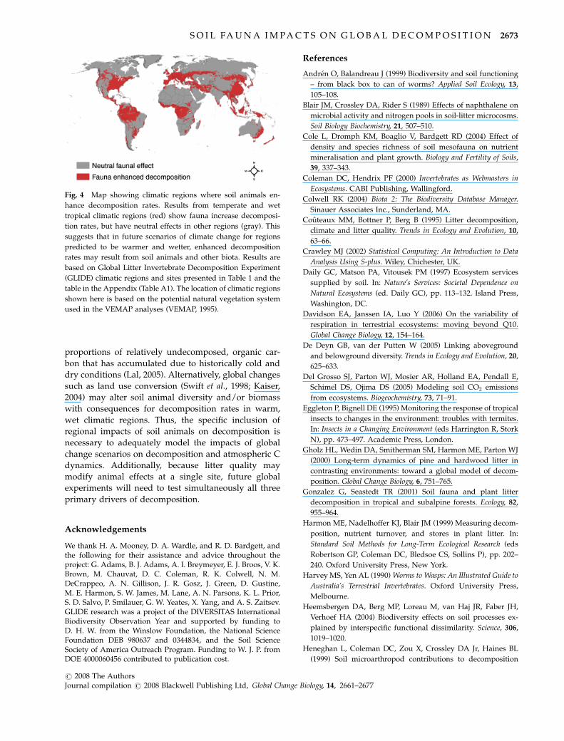
Fig. 4 Map showing climatic regions where soil animals en-

hance decomposition rates. Results from temperate and wet

tropical climatic regions (red) show fauna increase decomposi-

tion rates, but have neutral effects in other regions (gray). This

suggests that in future scenarios of climate change for regions

predicted to be warmer and wetter, enhanced decomposition

rates may result from soil animals and other biota. Results are

based on Global Litter Invertebrate Decomposition Experiment

(GLIDE) climatic regions and sites presented in Table 1 and the

table in the Appendix (Table A1). The location of climatic regions

shown here is based on the potential natural vegetation system

used in the VEMAP analyses (VEMAP, 1995).

S O I L FA U N A I M PA C T S O N G L O B A L D E C O M P O S I T I O N 2673

r 2008 The AuthorsJournal compilation r 2008 Blackwell Publishing Ltd, Global Change Biology, 14, 2661–2677

dynamics: tropical–temperate comparisons of a single sub-

strate. Ecology, 80, 1873–1882.

Kaiser J (2004) Wounding Earth’s fragile skin. Science, 304,

1616–1618.

Kibblewhite MG, Ritz K, Swift MJ (2008) Soil health in agricul-

tural systems. Philosophical Transactions of the Royal Society

Series B, 363, 685–701.

Lal R (2005) Forest soils and carbon sequestration. Forest Ecolo-

gical Management, 220, 242–258.

Lavelle P (1997) Faunal activities and soil processes: adaptive

strategies that determine ecosystem function. Advances in

Ecological Research, 27, 93–132.

Lavelle P, Bignell DE, Austen MC et al. (2004) Connecting soil

and sediment biodiversity: the role of scale and implications

for management. In: Sustaining Biodiversity and Ecosystem

Services in Soils and Sediments (ed. Wall DH), pp. 193–224.

Island Press, Washington.

Lawton JH, Bignell DE, Bolton B et al. (1998) Biodiversity

inventories, indicator taxa and effects of habitat modification

in tropical forest. Nature, 391, 72–76.

Leemans R (1990) Possible changes in natural vegetation patterns due

to global warming. IIASA Working Paper WP-90-008. Interna-

tional Institute for Applied Systems Analysis, Laxenburg,

Austria.

Liski J, Nissinen A, Erhard M, Taskinen O (2003) Climatic effects

on litter decomposition from arctic tundra to tropical rain-

forest. Global Change Biology, 9, 575–584.

Loreau M, Naeem S, Inchausti P (2002) Biodiversity and Ecosystem

Functioning: Synthesis and Perspectives. Oxford University

Press, Oxford.

Maraun M, Schatz H, Scheu S (2007) Awesome or ordinary?

Global diversity patterns of oribatid mites. Ecography, 30,

209–216.

Moorhead DL, Currie WS, Rastetter EB, Parton WJ, Harmon ME

(1999) Climate and litter quality controls on decomposition: an

analysis of modeling approaches. Global Biogeochemical Cycling,

13, 575–589.

Naeem S, Wright JP (2003) Disentangling biodiversity effects on

ecosystem functioning: deriving solutions to a seemingly

insurmountable problem. Ecology Letters, 6, 567–579.

Oliver I, Pik A, Britton D, Dangerfield JM, Colwell RK, Beattie AJ

(2000) Virtual biodiversity assessment systems. BioScience, 50,

441–450.

Parton WJ (1996) The CENTURY model. In: Evaluation of Soil

Organic Matter Models Using Existing Long-term Datasets (eds

Powlson DS, Smith P, Smith JU), pp. 283–293. Springer, Berlin.

Parton WJ, Silver WL, Burke IC et al. (2007) Global-scale simila-

rities in nitrogen release patterns during long-term decom-

position. Science, 315, 361–364.

Preston CM, Trofymow JA, Flanagan LB (2006) Decomposition,

d13C, and the ‘‘lignin paradox’’. Canadian Journal of Soil Science,

86, 235–245.

Preston CM, Trofymow JA, Sayer BG, Niu J (1997) 13C nuclear

magnetic resonance spectroscopy with cross-polarization and

magic-angle spinning investigation of the proximate-analysis

fractions used to assess litter quality in decomposition studies.

Canadian Journal of Botany, 75, 1601–1613.

Schimel DS, Alvves D, Enting I, Heimann M, Joos F, Raymond D,

Wigley T (1996) CO2 and the carbon cycle. In: Climate Change

1995 (eds Houghton J, Filho LM, Callander BA, Harris N,

Kattenberg A, Maskell K), pp. 76–86. Cambridge University

Press, Cambridge.

St. John MG, Wall DH, Behan-Pelletier V (2006) Does plant

species co-occurrence influence soil mite diversity? Ecology,

87, 625–633.

Swift MJ, Andren O, Brussaard L et al. (1998) Global change, soil

biodiversity, and nitrogen cycling in terrestrial ecosystems:

three case studies. Global Change Biology, 4, 729–743.

Swift MJ, Heal OW, Anderson JM (1979) Decomposition in Terres-

trial Ecosystems. Blackwell Scientific, Oxford.

Swift MJ, Izac A-MN, Van Noordwijk M (2004) Biodiversity and

ecosystem services in agricultural landscapes – are we asking

the right questions? Agriculture, Ecosystems & Environment, 104,

113–134.

Trofymow JA, Moore TR, Titus B et al. (2002) Rates of litter

decomposition over 6 years in Canadian forests: influence of

litter quality and climate. Canadian Journal of Forestry Research,

32, 789–804.

VEMAP (1995) Vegetation/ecosystem modeling and analysis

project: comparing biogeography and biogeochemistry mod-

els in a continental-scale study of terrestrial ecosystem

responses to climate-change and CO2 doubling. Global Biogeo-

chemical Cycling, 9, 407–437.

Wall DH, (ed) (2004) Sustaining Biodiversity and Ecosystem

Services in Soils and Sediments. Island Press, Washington, DC.

Wardle DA (1995) Impacts of disturbance on detritus food webs

in agro-ecosystems of contrasting tillage and weed manage-

ment practices. Advances in Ecological Research, 26, 105–185.

Wardle DA (2002) Communities and Ecosystems: Linking the Above-

ground and Belowground Components. Princeton University

Press, Princeton.

Appendix

Monthly values for mean precipitation (Precip, cm), maximum

(Tmax) and minimum (Tmin) temperatures ( 1C), and monthly

climate decomposition index (CDI) calculation for each site.

Italicised values indicate actual months in the field (see Table 2)

for sites where litterbags were in the field for o12 months. For

these sites only the italicised values were used to calculate the

mean CDI. See Table 1 for explanation of site codes.

2674 D . H . WA L L et al.

r 2008 The AuthorsJournal compilation r 2008 Blackwell Publishing Ltd, Global Change Biology, 14, 2661–2677

Table A1

Site

code Variable January February March April May June July August September October November December

TAS

1 & 2

Precip 8.04 6.30 4.71 8.28 8.17 9.55 12.18 12.22 9.62 11.78 8.94 10.32

Tmax 17.00 17.10 15.60 13.30 10.20 8.20 8.00 8.60 9.70 11.80 13.70 15.20

Tmin 8.20 8.50 7.40 6.10 4.20 2.40 2.20 2.60 3.30 4.40 5.90 7.40

CDI 0.3055 0.3223 0.2673 0.3177 0.2588 0.213 0.2077 0.2192 0.2411 0.2817 0.3048 0.3139

MAN Precip 19.82 21.85 25.92 25.07 27.04 19.87 17.69 10.50 9.36 8.58 11.94 13.46

Tmax 29.95 30.05 30.25 30.00 29.90 30.00 29.40 30.45 31.70 31.90 30.95 30.15

Tmin 21.95 22.05 22.25 22.00 22.10 22.00 21.40 22.45 21.90 22.20 22.95 22.15

CDI 0.8796 0.9023 0.9322 0.9283 0.9286 0.9277 0.9054 0.7639 0.6977 0.5399 0.6748 0.8926

RUB Precip 19.14 10.56 13.41 6.01 3.61 1.45 0.93 1.98 6.16 9.83 19.48 24.20

Tmax 29.93 30.15 29.85 28.78 27.13 25.75 25.13 26.15 26.88 28.08 28.55 28.68

Tmin 19.93 20.15 19.85 18.78 16.13 13.75 13.13 14.15 15.88 18.13 19.15 19.63

CDI 0.7624 0.6058 0.6773 0.4945 0.3025 0.1041 0.0529 0.1518 0.3905 0.5827 0.8606 0.8725

BON Precip 0.03 0.03 1.48 3.88 9.14 13.60 19.63 26.02 15.23 5.61 0.88 0.21

Tmax 32.30 35.60 36.60 36.40 34.60 31.60 29.50 28.00 29.80 32.30 33.70 32.70

Tmin 17.30 20.00 23.60 25.40 24.60 22.20 21.50 21.20 21.40 21.50 19.70 18.10

CDI 0.0296 0.0315 0.0831 0.1934 0.6064 0.8505 0.9154 0.8955 0.8907 0.3882 0.0619 0.0338

INU Precip 0.86 0.83 1.00 0.78 1.28 1.35 2.22 2.71 2.34 1.94 1.07 0.96

Tmax �25.70 �24.80 �20.50 �12.80 �3.00 7.30 13.00 11.10 3.70 �4.70 �17.90 �23.30

Tmin �31.90 �31.60 �28.30 �21.40 �9.20 1.50 5.60 5.30 �0.30 �8.90 �23.90 �29.50

CDI 0.0004 0.0005 0.0005 0.0014 0.0224 0.0354 0.0852 0.194 0.1414 0.0488 0.0005 0.0005

YUK Precip 1.68 1.58 1.10 0.51 1.48 3.49 5.21 2.83 2.83 1.67 2.23 1.91

Tmax �14.30 �12.00 �4.80 2.60 9.00 13.80 16.00 14.80 8.70 0.30 �10.20 �11.90

Tmin �23.90 �22.80 �16.80 �8.20 �2.20 1.40 4.40 3.00 �1.50 �6.70 �17.80 �20.90

CDI 0.004 0.004 0.0143 0.0111 0.0272 0.0839 0.1846 0.1256 0.148 0.0786 0.0121 0.0067

TOP Precip 5.34 2.49 2.54 1.74 3.38 5.61 4.32 3.43 3.78 4.22 6.36 5.58

Tmax �5.90 �3.10 2.80 7.70 12.50 16.00 18.60 18.60 14.60 7.10 �0.50 �4.60

Tmin �13.30 �13.50 �8.20 �3.10 1.10 4.60 7.00 6.80 2.80 �1.10 �6.10 �11.00

CDI 0.0321 0.0393 0.0683 0.0438 0.0941 0.188 0.1764 0.1732 0.1809 0.1666 0.0803 0.0422

LET Precip 1.63 1.79 2.21 3.02 5.38 7.80 6.85 5.86 3.86 2.34 2.03 1.57

Tmax �0.70 �0.40 5.50 11.20 16.30 19.90 21.80 21.40 18.10 12.10 3.00 �0.80

Tmin �11.90 �12.60 �6.50 �1.40 3.10 7.30 8.80 7.80 3.90 �1.30 �7.40 �11.60

CDI 0.0441 0.0405 0.0633 0.0861 0.1854 0.307 0.2853 0.3087 0.1788 0.1432 0.0821 0.0476

VAN Precip 27.20 16.86 18.12 13.91 11.75 11.95 7.15 7.22 6.14 18.62 31.07 26.02

Tmax 1.80 2.60 5.10 8.40 12.40 15.40 18.50 19.20 16.50 9.80 3.80 1.30

Tmin �2.80 �3.20 �1.30 1.60 4.20 7.00 9.90 10.00 7.30 3.60 �0.40 �2.70

CDI 0.1139 0.1154 0.1475 0.2058 0.25 0.3764 0.391 0.3617 0.2831 0.2459 0.144 0.1101

ROC Precip 10.85 9.27 7.60 8.35 8.18 9.90 8.44 10.66 10.04 11.26 10.90 9.74

Tmax �6.50 �8.40 �2.90 3.00 8.90 14.90 18.70 18.70 14.10 8.20 1.90 �3.40

Tmin �14.90 �17.00 �11.70 �3.60 0.50 5.10 8.90 10.30 5.70 1.40 �4.10 �9.80

CDI 0.0221 0.0125 0.0452 0.1133 0.174 0.3148 0.3839 0.5064 0.3432 0.2024 0.1051 0.0502

ONE Precip 1.53 1.58 2.33 2.37 3.84 7.16 5.41 3.16 3.40 1.62 1.88 1.68

Tmax �4.90 �3.10 4.60 11.30 17.30 22.40 24.50 24.50 19.20 11.30 1.10 �4.00

Tmin �15.50 �15.50 �7.40 �1.50 4.10 9.00 10.30 9.50 4.00 �3.10 �10.30 �15.40

CDI 0.0269 0.0242 0.0627 0.0661 0.1236 0.3062 0.254 0.1412 0.127 0.0807 0.0589 0.0248

XIS Precip 1.56 2.90 2.60 6.59 14.84 18.07 25.44 26.50 16.57 9.29 4.73 3.11

Tmax 21.40 23.70 26.00 28.90 28.50 27.40 26.40 26.90 26.90 25.00 22.50 20.30

Tmin 9.80 10.10 12.00 15.70 18.70 21.00 20.40 20.10 19.10 17.00 13.90 9.90

CDI 0.1066 0.1932 0.1456 0.3517 0.7411 0.8761 0.8652 0.8607 0.8512 0.7282 0.399 0.2113

BOG Precip 4.56 9.16 11.62 13.87 11.56 5.81 6.23 6.31 13.49 13.13 14.30 7.43

Tmax 19.60 19.30 19.30 19.20 19.60 18.80 18.30 18.40 18.90 18.30 18.50 18.80

Tmin 9.60 10.10 10.50 11.20 12.20 11.20 10.70 10.40 10.50 10.10 10.30 9.60

CDI 0.261 0.4723 0.4294 0.5169 0.5202 0.3416 0.3739 0.3617 0.5269 0.4776 0.5048 0.3588

Continued

S O I L FA U N A I M PA C T S O N G L O B A L D E C O M P O S I T I O N 2675

r 2008 The AuthorsJournal compilation r 2008 Blackwell Publishing Ltd, Global Change Biology, 14, 2661–2677

Table A1. (Contd.)

Site

code Variable January February March April May June July August September October November December

BIO Precip 3.11 3.33 4.58 4.77 6.50 8.97 8.34 7.65 4.87 3.09 4.45 5.13

Tmax 0.80 1.70 6.40 12.10 17.30 19.20 22.40 22.20 17.10 12.10 3.80 0.70

Tmin �3.60 �3.50 �0.60 2.30 7.10 10.00 12.40 12.00 8.50 3.70 �0.20 �2.50

CDI 0.1024 0.1127 0.151 0.1733 0.2555 0.4353 0.4473 0.5156 0.3649 0.2313 0.1474 0.1079

SUM Precip 3.11 3.33 4.58 4.77 6.50 8.97 8.34 7.65 4.87 3.09 4.45 5.13

Tmax 0.80 1.70 6.40 12.10 17.30 19.20 22.40 22.20 17.10 12.10 3.80 0.70

Tmin �3.60 �3.50 �0.60 2.30 7.10 10.00 12.40 12.00 8.50 3.70 �0.20 �2.50

CDI 0.1024 0.1127 0.151 0.1733 0.2555 0.4353 0.4473 0.5156 0.3649 0.2313 0.1474 0.1079

KOM Precip 2.28 2.89 3.40 3.96 6.28 7.51 5.31 5.72 5.03 3.27 4.27 4.09

Tmax 1.20 3.10 7.90 14.70 18.80 21.60 25.30 24.70 19.10 13.90 5.10 1.40

Tmin �2.80 �2.30 1.10 4.50 9.60 12.20 15.10 14.30 10.90 5.30 1.10 �1.80

CDI 0.0987 0.1266 0.1519 0.1572 0.3186 0.4368 0.2992 0.4443 0.3772 0.2573 0.1698 0.1166

PAL Precip 2.28 2.89 3.40 3.96 6.28 7.51 5.31 5.72 5.03 3.27 4.27 4.09

Tmax 1.20 3.10 7.90 14.70 18.80 21.60 25.30 24.70 19.10 13.90 5.10 1.40

Tmin �2.80 �2.30 1.10 4.50 9.60 12.20 15.10 14.30 10.90 5.30 1.10 �1.80

CDI 0.0987 0.1266 0.1519 0.1572 0.3186 0.4368 0.2992 0.4443 0.3772 0.2573 0.1698 0.1166

GIE Precip 5.41 3.94 6.02 4.70 5.28 7.61 7.54 5.95 6.05 4.15 5.09 6.59

Tmax 1.90 2.20 6.80 11.20 16.60 18.20 21.40 21.10 15.80 11.40 5.60 2.40

Tmin �1.30 �2.20 0.60 3.20 7.60 10.40 13.40 12.30 9.00 5.60 1.40 �0.60

CDI 0.1262 0.1258 0.1681 0.1857 0.2253 0.4134 0.4676 0.4392 0.4065 0.2731 0.1776 0.1329

JEN Precip 3.86 3.80 4.58 4.18 4.44 7.44 7.23 5.37 4.78 2.92 4.74 5.29

Tmax 1.70 2.30 7.30 12.10 17.70 19.60 22.50 22.10 17.20 12.20 5.20 2.20

Tmin �2.10 �2.70 0.10 3.30 7.30 10.20 13.10 12.50 9.00 5.00 0.80 �1.00

CDI 0.1194 0.123 0.1489 0.1677 0.2148 0.3764 0.4405 0.3962 0.3823 0.2524 0.1683 0.1283

KEN Precip 5.86 11.23 14.43 27.27 21.95 15.29 11.67 17.35 15.51 20.92 13.21 10.89

Tmax 28.40 28.90 29.10 27.70 26.40 26.10 26.00 26.70 28.00 28.20 28.20 28.10

Tmin 12.80 13.10 14.10 14.50 14.40 14.10 13.60 13.30 13.00 14.20 14.20 12.90

CDI 0.3105 0.5301 0.6646 0.7941 0.7647 0.7106 0.6566 0.7255 0.6663 0.7021 0.7107 0.4515

MAL Precip 7.29 9.96 11.03 12.12 30.39 23.80 23.18 32.12 27.61 29.60 30.51 23.10

Tmax 25.70 25.50 26.60 27.20 27.20 26.30 26.00 26.00 26.20 26.80 26.40 26.30

Tmin 19.50 18.50 19.00 19.20 19.40 19.10 19.20 18.80 19.20 19.20 19.00 19.70

CDI 0.6476 0.5711 0.6202 0.6266 0.8543 0.8334 0.8419 0.8357 0.8452 0.8543 0.8453 0.7291

NAM Precip 0.00 0.00 0.00 0.12 0.00 0.00 0.00 0.00 0.00 0.00 0.00 0.00

Tmax 19.60 22.90 27.80 32.90 37.00 40.10 39.20 38.30 36.60 32.00 26.10 20.40

Tmin 5.60 8.30 12.00 16.90 20.80 23.50 23.60 23.70 21.40 16.80 11.10 7.20

CDI 0.0144 0.0185 0.0242 0.0304 0.0317 0.033 0.0328 0.0327 0.0318 0.0287 0.0226 0.016

KUR Precip 4.38 3.28 3.81 5.47 5.90 8.82 6.24 5.91 7.03 5.10 4.75 4.48

Tmax �4.40 �4.10 1.50 10.90 18.10 22.20 22.60 22.30 15.90 8.30 �0.80 �4.60

Tmin �9.60 �9.30 �4.30 3.10 8.30 12.80 14.20 12.70 8.30 2.30 �4.60 �8.80

CDI 0.0515 0.0533 0.1045 0.2302 0.274 0.5028 0.4013 0.4099 0.3469 0.1913 0.0887 0.0496

SEN Precip 0.05 0.05 0.01 0.03 0.07 0.83 3.77 9.68 10.05 1.51 0.00 0.06

Tmax 30.55 32.30 34.60 35.75 37.20 37.05 34.20 33.55 33.85 35.65 33.75 30.90

Tmin 14.05 16.40 17.90 19.05 20.70 22.45 23.40 24.35 24.15 23.15 19.55 16.10

CDI 0.0277 0.0295 0.0302 0.0312 0.0325 0.0481 0.2005 0.6514 0.6796 0.0878 0.0304 0.0291

TAI Precip 12.43 16.25 21.71 16.03 22.45 24.85 14.98 22.23 25.08 11.91 12.14 8.15

Tmax 17.50 16.90 19.20 22.70 25.20 27.90 29.70 29.30 27.60 24.40 21.50 19.50

Tmin 12.30 11.50 13.40 16.70 19.60 22.10 23.70 23.50 21.80 18.80 16.10 13.70

CDI 0.5385 0.5123 0.6039 0.7267 0.8193 0.8577 0.8653 0.9358 0.8976 0.7332 0.6855 0.5995

CAR Precip 7.67 4.77 6.75 4.05 4.33 6.74 7.80 8.62 8.75 8.11 7.44 7.53

Tmax 5.70 5.20 9.30 11.70 16.70 18.00 21.40 21.00 16.90 13.50 8.90 6.20

Tmin 1.70 0.40 2.70 4.10 7.90 10.80 13.80 12.80 10.50 7.70 4.50 2.80

CDI 0.1827 0.1629 0.2007 0.1931 0.2128 0.3687 0.4696 0.4692 0.4874 0.3594 0.249 0.1972

Continued

2676 D . H . WA L L et al.

r 2008 The AuthorsJournal compilation r 2008 Blackwell Publishing Ltd, Global Change Biology, 14, 2661–2677

Table A1. (Contd.)

Site

code Variable January February March April May June July August September October November December

SIL Precip 9.09 6.01 5.35 5.97 4.15 4.72 4.89 4.88 6.27 8.44 6.38 7.96

Tmax 6.50 6.10 9.30 11.60 15.90 18.50 21.00 20.80 17.20 13.20 9.00 6.60

Tmin 1.50 0.70 2.50 3.60 6.70 9.30 12.00 11.20 8.80 6.20 3.20 1.60

CDI 0.1869 0.1654 0.2032 0.2279 0.1708 0.2172 0.2865 0.2965 0.3861 0.3361 0.2328 0.1876

COL Precip 0.85 1.33 3.58 3.54 6.30 6.23 4.20 4.06 3.38 2.31 1.88 0.88

Tmax 4.90 5.90 10.80 15.40 19.80 25.90 28.60 27.70 23.30 17.10 9.30 4.30

Tmin �8.90 �7.70 �3.40 0.20 5.40 10.70 12.80 12.30 7.10 0.90 �4.70 �9.10

CDI 0.032 0.0418 0.0804 0.0996 0.1988 0.2558 0.1512 0.1806 0.1857 0.1125 0.0918 0.0361

FLO Precip 6.81 5.47 8.36 4.79 7.77 18.94 17.67 19.10 17.74 10.62 6.45 3.67

Tmax 22.90 23.80 25.70 27.40 30.80 31.80 32.50 32.10 31.50 29.20 26.50 23.20

Tmin 11.50 11.80 13.70 15.20 18.60 21.60 22.50 22.50 22.50 19.20 16.30 12.00

CDI 0.4673 0.4399 0.4604 0.2806 0.4586 0.8612 0.9186 0.9172 0.9443 0.6969 0.5374 0.2893

S O I L FA U N A I M PA C T S O N G L O B A L D E C O M P O S I T I O N 2677

r 2008 The AuthorsJournal compilation r 2008 Blackwell Publishing Ltd, Global Change Biology, 14, 2661–2677