DOMAIN DECOMPOSITION TECHNIQUES AND ... - CIMEC
239
DOMAIN DECOMPOSITION TECHNIQUES AND DISTRIBUTED PROGRAMMING IN COMPUTATIONAL FLUID DYNAMICS by Rodrigo Rafael Paz A dissertation submitted to the Postgraduate Department of the FACULTAD DE INGENIER ´ IA Y CIENCIAS H ´ IDRICAS for partial fulfillment of the requirements for the degree of DOCTOR IN ENGINEERING Field of Computational Mechanics of the UNIVERSIDAD NACIONAL DEL LITORAL 2006
-
Upload
khangminh22 -
Category
Documents
-
view
2 -
download
0
Transcript of DOMAIN DECOMPOSITION TECHNIQUES AND ... - CIMEC

DOMAIN DECOMPOSITION TECHNIQUES AND
DISTRIBUTED PROGRAMMING IN
COMPUTATIONAL FLUID DYNAMICS
by
Rodrigo Rafael Paz
A dissertation submitted to the Postgraduate Department of the
FACULTAD DE INGENIERIA Y CIENCIAS HIDRICAS
for partial fulfillment of the requirements
for the degree of
DOCTOR IN ENGINEERING
Field of Computational Mechanics
of the
UNIVERSIDAD NACIONAL DEL LITORAL
2006


TECNICAS DE DESCOMPOSICION DE DOMINIOY PROGRAMACION DISTRIBUIDA EN
MECANICA DE FLUIDOS COMPUTACIONAL
por
Rodrigo Rafael Paz
Tesis remitida a la Comision de Posgrado de la
FACULTAD DE INGENIERIA Y CIENCIAS HIDRICAS
como parte de los requisitos para la obtencion
del grado de
DOCTOR EN INGENIERIA
Mencion Mecanica Computacional
de la
UNIVERSIDAD NACIONAL DEL LITORAL
2006


A Eliana y Guadalupe,
a mis Padres Nestor y Susana,
a mi Hermana Lici
y a la memoria de mi Abuelo Agustın.

Acknowledgments
I will always be in debt to Mario Storti for his advise, support and kindly guide during
the elaboration of this thesis at CIMEC. I have had the privilege to work and teach with
him along these years. Also, I would like to remark that Mario gives special and dedicated
support to every PhD student and researcher at CIMEC laboratory. He can stay by your
side (stuck on a chair) for hours discussing an idea or debugging a (frequently unfriendly)
code as he would be the writer.
I would like to express my deepest appreciation to Prof. Sergio Idelsohn for constant
encouragement. Prof. Idelsohn has given me special participation in one of the most
important projects in which the CIMEC laboratory has been involved. Special thanks to
Norberto Nigro for very insightful discussions and intense collaboration. Beto had always
been interested on my work.
The research documented in this dissertation has been supported by Consejo Nacional
de Investigaciones Cientıficas y Tecnicas (CONICET), the national council for the research
in Argentina.
I would like to name Professor Vitoriano Ruas from the Laboratoire de Modelisation en
Mecanique, Universite Pierre et Marie Curie (Paris VI) and Professor Grigori Panasenko
from the Equipe d’Analyse Numerique, Universite de Saint-Etienne, who gave me special
support during my stage at Paris and Saint-Etienne. It has been very fruitful to work
with them. I am grateful to Carlos Mendez for revising the manuscript of this thesis, for
his useful advices and for the amusing conversations at the river shore in Santa Fe while
eating the well-known choris.
To all my friends at CIMEC. I have had wonderful days working with them in an
enlightening environment.
To my friends, always.
Finally, I would like to express my deepest thanks to Eliana and Guadalupe, for being
always with me, for the love, forbearance and unconditional support. To my father and
mother, Nestor and Susana, and to my sister Lici. They have always taught me the
importance of studying and the freedom that a person needs to do what he believes. To
my grandfather Agustın, I have spent my happiest days with him. My family is the energy
that moves me through life.
Deo Gratias.

Agradecimientos
Estoy inmensamente agradecido a Mario Storti por su direccion, guıa, dedicacion y ayuda;
dejandome ir siempre en la direccion en que me sentıa con mayor confianza. Tambien por
haber confiado en mı para dar clases junto a el en la facultad. A Sergio Idelsohn por creer
en mı y darme participacion dentro de los proyectos en que trabaje durante la tesis. A
Norberto Nigro por las discusiones y charlas, y por haberse interesado siempre en lo que
estaba trabajando.
Quiero agradecerle a CONICET por su programa de soporte para las carreras de
doctorado.
Un agradecimiento especial al Profesor Vitoriano Ruas del Laboratoire de Modelisation
en Mecanique, Universite Pierre et Marie Curie (Paris VI) y al Profesor Grigori Panasenko
del Equipe d’Analyse Numerique, Universite de Saint-Etienne, por el inmenso apoyo
brindado durante mi estadıa en Paris y Saint-Etienne. El trabajo con ellos fue muy
enriquecedor.
Agradezco a Carlos Mendez por la revision del manuscrito de esta tesis y por las
excelentes discusiones que hemos tenido a lo largo de estos anos.
A todos los amigos del CIMEC con los que aprendı y me divertı en un ambiente muy
grato.
A mis amigos, siempre.
Finalmente quiero agradecer a Eliana y a Guadalupe por estar a mi lado siempre, por
el carino y apoyo incondicional y la paciencia grande que tienen. A mis Padres Nestor
y Susana y a mi Hermana Lici por haberme inculcado la importancia del estudio y la
libertad que una persona necesita para hacer lo que cree. A mi abuelo Agustın que
siempre me hizo feliz. Ellos son el motor indispensable para seguir siempre adelante.
Deo Gratias.


Author’s Legal Declaration
This dissertation have been submitted to the Postgraduate Department of the Facultad
de Ingenierıa y Ciencias Hıdricas for partial fulfillment of the requirements for the degree
of Doctor in Engineering - Field of Computational Mechanics of the Universidad Nacional
del Litoral. A copy of this document will be available at the University Library and it
will be subjected to the Library’s legal normative.
Some parts of the work presented in this thesis have been (or are going to be) published
in the following journals: International Journal for Numerical Methods in Engineering, In-
ternational Journal for Numerical Methods in Fluids, Journal of Parallel and Distributed
Computing, Journal of Sound and Vibration, Journal of Computational Methods in Sci-
ence and Engineering and Journal of Computational Physics.
Any comment about the ideas and topics discussed and developed through this docu-
ment will be highly appreciated.
Rodrigo Rafael PAZ
c© Copyright by Rodrigo Rafael PAZ – 2006
All Rights Reserved


Introduction
The large spread in length and time scales present in Computational Fluid Dynamics
(CFD) problems and its interaction with solid or elastic bodies (e.g., coupled surface-
subsurface flows, high speed wind flows around complex bodies, non-linear fluid-structure
interactions) requires a high degree of refinement in the finite element mesh and, then,
requires very large computational resources.
The solution of ‘Large Scale’ CFD problems has a particular challenge that is the
efficient use of the allowable computational resources [LTV97, SP96]. If no suitable nu-
merical techniques are used to reduce, optimize and/or simplify the problem at hand it
may be necessary to increase computational resources in order to handle the problem.
Newer technologies and even faster and powerful (super-)computers make that the prob-
lems to be resolved be even larger and complex (i.e., larger domains, larger number of
degree of freedom’s (dof’s), models with increasing number of evolution variables, coupled
interacting fields). That is why the mathematical models used nowadays could be more
complex and complete (from a physical point of view) making the simulations extensive
and complicated. The constraint on the allowable computer resources is always present
and that is the reason of the urgent development and verification of solution techniques
that exploit efficiently the potential of new computers and the possibility to obtain solu-
tions of high quality [PNS06] in a affordable simulation time (i.e., CPU time). This thesis
has been conceived based on that fact.
During last decades there have been developed and tested a wide diversity of linear sys-
tem ‘solvers’ and they have been applied to the resolution of ‘real world’ physics problems
by means of the discretization of coupled (or not) sets of non-linear Partial Differential
Equations (PDE’s) via the Finite Element Method (FEM), the Finite Difference Method
(FDM) and/or Finite Volume Method (FVM). Since no long time ago (even at present
days), it has been preferred the direct solution of these systems of equations instead of
iterative schemes due to its higher robustness and its predictable behavior. Nevertheless,
the increasing number of iterative techniques and the proposed improvements, jointly with
the need to solve larger problems in Computational Mechanics area have bent to the use
xi

xii
of this kind of schemes and the development of newer ones.
This trend has been taking place since early seventies when two crucial developments
marked up an inflection point in the solution techniques of ‘large scale’ systems of equa-
tions. On of these was the advantage of using ‘low density’ or ‘low sparsity’ matrices that
arise in FEM (as well as in FDM and FVM) when discretized PDE’s are stated. The other
was the development of iterative methods over the Krylov space (or sub-space) such as
Conjugate Gradients (CG) and Generalized Minimal Residuals (GMRes) [SS86, Saa00].
Gradually, iterative methods (and their variants such as preconditioning) have attained
popularity and have begun to be extensively used by the scientific community and software
developers. Particularly, there is a vast amount of written work on the use of CG methods
for solving large scale coercive systems such as those resulting from the discretization of
linear elastic problem, potential flows and heat conduction, among others.
Nowadays, very large scale systems that arise in the context of FEM treatment of non-
linear transient governing equations are solved in high performance computers (parallel
and vectorized architectures) by means of iterative methods due to less requirements in
communications between processor than those required by direct methods (such as LU
decomposition, multifrontal methods).
The iterative ‘Substructuring’ Method, or Domain Decomposition Method (DDM) and
iteration over the ’Schur Complement’ Matrix on non-overlapping sub-domains, lead to
a reduced system better suited (i.e., lower condition number κ(A) and better eigenvalue
distribution) for Krylov-based iterative solution than the global solution. In Schur com-
plement domain decomposition general method, the condition number is lowered (∝ 1/h
vs ∝ 1/h2 for the global system, h being the mesh size) and the computational cost per
iteration is not so high once the sub-domain matrices have been factorized.
Iterative substructuring methods rely on a non-overlapping partition into sub-domains
(substructures). The efficiency of these methods can be further improved by using pre-
conditioners [LTV97]. Once the degrees of freedom inside the substructures have been
eliminated by block Gaussian elimination (or other algorithm), a preconditioner for the
resulting Schur complement system is built with matrix blocks relative to a decompo-
sition of interface finite element functions into subspaces related to geometrical objects
(vertices, edges, faces, single substructures) or simply by the coefficients of sub-domain
matrices near the interface. Iterative methods like CG and GMRes are then employed.
Early works, such as [BPS86, BPS89], have influenced most of the later work in the field.
They proposed two spaces for the coarse problem. One of their coarse spaces is given in
terms of the averages of the nodal values over the entire substructure boundaries ∂Ωi.
The other space is defined by extending the wire basket (we recall that the wire basket is

xiii
the union of the boundaries of the faces which separate the substructures) values as a two
dimensional discrete harmonic function onto the faces, and then as a discrete harmonic
function into the interiors of the sub-domains.
For self-adjoint positive semidefinite problems, Neumann-Neumann preconditioner is
the most classical one. From a mathematical point of view, the preconditioner is defined
by approximating the inverse of the global Schur complement matrix by the weighted sum
of local Schur complement matrices. From a physical point of view, Neumann-Neumann
preconditioner is based on splitting the flux applied to the interface in the preconditioning
step and solving local Neumann problems in each sub-domain. This strategy is good only
for symmetric operators.
Another family of DDM, the overlapping Schwarz domain decomposition schemes,
have also been extensively used in computational mechanics. A good introduction and
applications of these methods is presented by Smith and coworkers in Reference [SBrG96].
In the CFD area, Rachowicz [Rac97] applied successfully the GMRes solver with a domain
decomposition Schwarz-type preconditioner in the solution of hypersonic high Reynolds
number flows with strong shock-boundary layer interaction.
The main purpose of the present thesis work is the efficient solution of large scale
problems arising in Computational Fluid Dynamics challenge problems, the proposi-
tion of new ideas in preconditioning techniques, the implementation of such ideas in a
parallel multiphysics C++ code using the message passing paradigm via MPI/PETSc li-
braries [GLS94, BGCMS04] and its evaluation on a Beowulf class cluster [SSBS99]. These
topics are presented in the first part of this work. The second part is devoted to the
application of the algorithm proposed in the first part (§I) to the solution of more gen-
eral/complex problems like the wave absorption on fictitious boundaries and the resolution
of fluid-structure problems in the supersonic regime of a compressible fluid flow.


Introduccion
La diversidad de escalas de tiempo y de espacio presentes en problemas relacionados con la
mecanica de fluidos y su interaccion con cuerpos solidos (e.g., problemas de la hidrologıa
superficial y subterranea acoplados o no, flujo de viento alrededor de cuerpos, edificios
o vehıculos, etc.) requiere un alto grado de refinamiento en las mallas utilizadas en el
metodo de elementos finitos, y por lo tanto, demanda grandes recursos computacionales.
La solucion de problemas en ‘gran escala’ en la mecanica computacional tiene un
desafıo particular y es el de utilizar eficientemente los recursos disponibles [LTV97, SP96].
Si no se utilizan adecuadas tecnicas numericas para reducir, optimizar y/o simplificar
el problema, es menester contar con grandes recursos computacionales para tratar el
problema. Por otro lado, el auge de computadoras cada vez mas rapidas y con mayor
capacidad de calculo hace que los problemas que se quieren resolver sean cada vez mas
grandes y complejos (i.e., mayores y mas variadas escalas, acople de distintos campos,
modelos que tengan en cuenta otras variables y su evolucion e interaccion con las demas,
etc.). Es ası que los modelos matematicos son cada vez mas complejos y sofisticados,
haciendo que las simulaciones de los sistemas resultantes sean extensas y complicadas.
La restriccion sobre los recursos computacionales disponibles esta siempre presente y por
eso la urgencia en el desarrollo y verificacion de tecnicas de solucion capaces de explotar
eficientemente el potencial de las modernas computadoras y la posibilidad de obtener
soluciones de buena calidad en un tiempo aceptable de simulacion (tiempo de CPU). La
presente tesis nace de esta necesidad.
Durante varias decadas se han desarrollado y probado tecnicas concernientes a la
solucion de problemas lineales que son resultado de la aplicacion del metodo de elementos
finitos (MEF) a ecuaciones diferenciales en derivadas parciales (EDDP) que tratan de
describir un conjunto de eventos de la fısica (e.g., mecanica de cuerpos solidos, dinamica
estructural, dinamica de fluidos, etc.). Hasta no hace mucho tiempo, la solucion directa de
estos sistemas era preferida a la solucion iterativa debido a su mayor robustez y al caracter
predictivo de su comportamiento. Sin embargo, la gran cantidad de tecnicas iterativas que
han sido desarrolladas, conjuntamente con la necesidad de resolver sistemas de ecuaciones
xv
xvi
cada vez mas grandes en diferentes arquitecturas han dado como resultado una inclinacion
al uso de este tipo de tecnicas y al desarrollo de nuevas.
Esta tendencia se viene dando desde 1970 cuando dos importantes desarrollos mar-
caron un punto de inflexion en la solucion de grandes sistemas de ecuaciones. Uno fue la
explotacion de la ‘baja densidad’ (por sparsity, matrices ralas, matrices con tasa de llenado
baja) de los sistemas que resultan de la aplicacion del MEF (como ası tambien del metodo
de diferencias finitas MDF) a las EDDP. El otro fue el desarrollo de metodos tales como los
de Krylov (o metodos tipo gradientes conjugados precondicionados). Gradualmente los
metodos iterativos (precondicionamiento e iteracion en el espacio de Krylov) comenzaron
a aproximarse en calidad a las soluciones provistas por metodos directos. Particular-
mente, mucho se ha escrito sobre el metodo de gradientes conjugados precondicionado
para sistemas lineales simetricos que resultan de operadores simetricos (e.g., elasticidad
lineal y no lineal, flujo potencial, etc.).
Hoy, los grandes sistemas de ecuaciones obtenidos de las EDDP no lineales medi-
ante el MEF para problemas transitorios en dos y tres dimensiones donde pueden haber
varias incognitas por nodo, son resueltos con metodos iterativos en computadoras de alta
performance (arquitecturas paralelas o vectoriales) debido a que requieren mucha menor
comunicacion entre los procesadores que la necesaria en metodos directos donde la solucion
de cada una de las incognitas esta acoplada con las demas.
El metodo de subestructuracion (o metodo de descomposicion de dominios e iteracion
sobre la matriz complemento de Schur para dominios no solapados) conduce a sistemas
reducidos mejor condicionados para la solucion mediante metodos de Krylov. El numero
de condicion de estos problemas se ve disminuido en un factor 1/h (∝ 1/h vs ∝ 1/h2
para el sistema global, siendo h la dimension caracterıstica de la malla) y el costo com-
putacional por iteracion no se ve encarecido debido a que las matrices correspondientes a
los grados de libertad de los subdominios (grados de libertad interiores) ya han sido
factorizadas. La eficiencia de estos metodos puede ser mejorada mediante el uso de
precondicionadores [Meu99, Man93, BPS86, Cro02]. Diferentes tecnicas de precondi-
cionamiento han sido propuestas y la reduccion del numero de condicion de las matrices ha
sido demostrada en el marco de ecuaciones diferenciales lineales elıpticas (e.g., precondi-
cionadores del tipo wire basket, Neumann-Neumann y sus variantes para los problemas
de elasticidad y flujo de Stokes).
En este trabajo se buscara solucionar eficientemente los sistemas de ecuaciones prove-
nientes de la discretizacion mediante el MEF o MDF de ecuaciones diferenciales no lineales
en derivadas parciales que representan modelos numericos de problemas reales (como los
descriptos arriba) considerados un desafıo para los metodos computacionales actuales. El

xvii
objetivo es tambien el desarrollo de un codigo de elementos finitos orientado a objetos
(que reduce drasticamente las dependencias de implementacion entre subsistemas y que
conduce al principio de reusabilidad de disenos de interfaces) que resuelva problemas de
la mecanica de fluidos computacional en gran escala en forma distribuida mediante la
tecnica de paso de mensajes (MPI/PETSc [GLS94, BGCMS04]). Esta tecnica es amplia-
mente explotable en arquitecturas de computadoras paralelas, tales como la de ‘clusters’
Beowulf [SSBS99]. En la primer parte de esta tesis seran expuestos y desarrollados los
topicos relacionados con los metodos de descomposicion de dominios y su desempeno en
problemas clasicos de la mecanica de fluidos computacional. La segunda parte esta ded-
icada a la aplicacion del algoritmo propuesto en la primera parte (§I) a la solucion de
problemas mas generales/complejos como lo es la absorcion de ondas en fronteras ficticias
y la solucion de problemas de interaccion fluido/estructura para el flujo supersonico de
un fluido compresible.


Contents
I Domain Decomposition Methods 1
1 Preliminaries 3
1.1 Solution of Linear Systems . . . . . . . . . . . . . . . . . . . . . . . . . . . 7
1.1.1 Perturbation Theory . . . . . . . . . . . . . . . . . . . . . . . . . . 7
1.1.2 Condition Number . . . . . . . . . . . . . . . . . . . . . . . . . . . 8
1.2 Preconditioning . . . . . . . . . . . . . . . . . . . . . . . . . . . . . . . . . 8
1.3 Basic Iterative Method . . . . . . . . . . . . . . . . . . . . . . . . . . . . . 9
1.3.1 Optimal Iteration Methods . . . . . . . . . . . . . . . . . . . . . . . 11
2 The ‘Interface Strip Preconditioner’ for Domain Decomposition Meth-
ods 13
2.1 Introduction . . . . . . . . . . . . . . . . . . . . . . . . . . . . . . . . . . . 14
2.2 Schur Complement Domain Decomposition Method . . . . . . . . . . . . . 18
2.2.1 The Steklov Operator . . . . . . . . . . . . . . . . . . . . . . . . . . 20
2.2.2 Eigenvalues of Steklov Operator . . . . . . . . . . . . . . . . . . . . 21
2.3 Preconditioners for the Schur Complement Matrix . . . . . . . . . . . . . . 24
2.3.1 The Neumann-Neumann Preconditioner . . . . . . . . . . . . . . . 25
2.3.2 The Interface Strip Preconditioner (ISP) . . . . . . . . . . . . . . . 27
2.4 The Advective-Diffusive Case . . . . . . . . . . . . . . . . . . . . . . . . . 28
2.5 Implementation of the Neumann-Neumann Preconditioner . . . . . . . . . 36
2.5.1 The Balancing Neumann-Neumann Version . . . . . . . . . . . . . . 38
2.6 The Interface Strip Preconditioner: Solution of the Strip Problem . . . . . 42
2.6.1 Implementation Details of the IISD Solver . . . . . . . . . . . . . . 44
2.7 Classical Overlapping Domain Decomposition
Method: Alternating Schwarz Methods . . . . . . . . . . . . . . . . . . . . 46
2.8 Conclusions . . . . . . . . . . . . . . . . . . . . . . . . . . . . . . . . . . . 48
xix

xx CONTENTS
3 Numerical Tests 49
3.1 Numerical Examples in Sequential Environments . . . . . . . . . . . . . . . 50
3.1.1 The Poisson’s Problem . . . . . . . . . . . . . . . . . . . . . . . . . 50
3.1.2 The Scalar Advective-Diffusive Problem . . . . . . . . . . . . . . . 51
3.1.3 The Hypersonic Flow Over a Flat Plate Test . . . . . . . . . . . . . 53
3.2 Numerical Examples in Parallel Environment . . . . . . . . . . . . . . . . . 60
3.2.1 The Poisson’s Problem . . . . . . . . . . . . . . . . . . . . . . . . . 62
3.2.2 The Scalar Advective-Diffusive Problem . . . . . . . . . . . . . . . 63
3.2.3 The Coupled Hydrological Flow Model . . . . . . . . . . . . . . . . 65
3.2.4 The Stokes Flow in a Long Horizontal Channel . . . . . . . . . . . 74
3.2.5 The Viscous Incompressible Navier-Stokes Flow Around an Infinite
Cylinder . . . . . . . . . . . . . . . . . . . . . . . . . . . . . . . . . 82
3.2.6 Navier-Stokes Flow Using the Fractional Step Scheme. The Lid
Driven Cavity . . . . . . . . . . . . . . . . . . . . . . . . . . . . . . 86
3.2.7 The Wind Flow Around a 3D Immersed Body.
The AHMED Model . . . . . . . . . . . . . . . . . . . . . . . . . . 92
3.3 Conclusions . . . . . . . . . . . . . . . . . . . . . . . . . . . . . . . . . . . 97
II Applications and Usage 99
4 Dynamic Boundary Conditions in CFD 101
4.1 Introduction . . . . . . . . . . . . . . . . . . . . . . . . . . . . . . . . . . . 102
4.2 General Advective-Diffusive Systems of Equations . . . . . . . . . . . . . . 104
4.2.1 Linear Advection-Diffusion Model . . . . . . . . . . . . . . . . . . . 105
4.2.2 Gas Dynamic Equations . . . . . . . . . . . . . . . . . . . . . . . . 105
4.2.3 Shallow Water Equations . . . . . . . . . . . . . . . . . . . . . . . . 106
4.2.4 Channel Flow . . . . . . . . . . . . . . . . . . . . . . . . . . . . . . 106
4.3 Variational Formulation . . . . . . . . . . . . . . . . . . . . . . . . . . . . 107
4.4 Absorbing Boundary Conditions . . . . . . . . . . . . . . . . . . . . . . . . 107
4.4.1 Advective-Diffusive Systems in 1D . . . . . . . . . . . . . . . . . . . 109
4.4.2 Linear 1D Absorbing Boundary Conditions . . . . . . . . . . . . . . 110
4.4.3 Multidimensional Problems . . . . . . . . . . . . . . . . . . . . . . 112
4.4.4 Absorbing Boundary Conditions for Nonlinear Problems . . . . . . 114
4.4.5 Riemann Based Absorbing Boundary Conditions . . . . . . . . . . . 114
4.4.6 Absorbing Boundary Conditions Based on Last State . . . . . . . . 116
4.4.7 Imposing Nonlinear Absorbing Boundary Conditions . . . . . . . . 117

CONTENTS xxi
4.4.8 Numerical Example. Viscous Compressible Subsonic Flow Over a
Parabolic Bump . . . . . . . . . . . . . . . . . . . . . . . . . . . . . 121
4.5 Dynamically Varying Boundary Conditions . . . . . . . . . . . . . . . . . . 121
4.5.1 Varying Boundary Conditions in External Aerodynamics . . . . . . 121
4.5.2 Aerodynamics of Falling Objects . . . . . . . . . . . . . . . . . . . 124
4.6 Conclusions . . . . . . . . . . . . . . . . . . . . . . . . . . . . . . . . . . . 127
5 Strong Coupling Strategy for Fluid-Structure Interaction Problems in
Supersonic Regime Via Fixed Point Iteration 131
5.1 Introduction . . . . . . . . . . . . . . . . . . . . . . . . . . . . . . . . . . . 132
5.2 Strongly Coupled Partitioned Algorithm Via Fixed Point Iteration . . . . . 133
5.2.1 Notes on the Fluid/Structure Interaction (FSI) Algorithm . . . . . 135
5.3 Description of Test Case . . . . . . . . . . . . . . . . . . . . . . . . . . . . 137
5.3.1 Dimensionless Parameters . . . . . . . . . . . . . . . . . . . . . . . 138
5.3.2 Houbolt’s Model . . . . . . . . . . . . . . . . . . . . . . . . . . . . 139
5.3.3 FSI Code Results . . . . . . . . . . . . . . . . . . . . . . . . . . . . 144
5.4 Stability of the Weak/Strong Staged Coupling Outside the Flutter Region 151
5.5 Conclusions . . . . . . . . . . . . . . . . . . . . . . . . . . . . . . . . . . . 156
III Final Conclusions 157
6 Overview and Final Remarks 159
IV Appendix 161
A Functional Spaces 163
A.1 Some Used Sobolev Spaces . . . . . . . . . . . . . . . . . . . . . . . . . . . 163
A.2 Extension to Vector-Valued Functions . . . . . . . . . . . . . . . . . . . . . 164
B Resumen extendido en castellano 167
B.1 El Metodo de Descomposicion de Dominios en Mecanica de Fluidos Com-
putacional . . . . . . . . . . . . . . . . . . . . . . . . . . . . . . . . . . . . 167
B.2 Ecuaciones de Gobierno . . . . . . . . . . . . . . . . . . . . . . . . . . . . 169
B.2.1 Propiedades Continuas de los Fluidos . . . . . . . . . . . . . . . . . 170
B.2.2 Campos Lagrangianos y Eulerianos . . . . . . . . . . . . . . . . . . 171
B.2.3 La Ecuacion de Continuidad . . . . . . . . . . . . . . . . . . . . . . 174

xxii CONTENTS
B.2.4 La Ecuacion de Cantidad de Movimiento . . . . . . . . . . . . . . . 175
B.2.5 Las Ecuaciones de Navier-Stokes en Sistemas de Referencia No Iner-
ciales . . . . . . . . . . . . . . . . . . . . . . . . . . . . . . . . . . . 176
B.2.6 Las Ecuaciones de Navier-Stokes Incompresibles . . . . . . . . . . . 177
B.3 Formulacion de otros Modelos Matematicos a Tratar . . . . . . . . . . . . 179
B.3.1 Problemas Hidrologicos . . . . . . . . . . . . . . . . . . . . . . . . . 179
B.4 Computacion de Alta Performance . . . . . . . . . . . . . . . . . . . . . . 182
B.4.1 Resolucion Numerica del Modelo de CFD/Hidrologıa Superficial y
Subterranea . . . . . . . . . . . . . . . . . . . . . . . . . . . . . . . 182
B.4.2 Solucion de Grandes Sistemas de Ecuaciones . . . . . . . . . . . . . 183
B.4.3 Metodos de Descomposicion de Dominio . . . . . . . . . . . . . . . 185
B.4.4 Precondicionamiento . . . . . . . . . . . . . . . . . . . . . . . . . . 188
B.4.5 Implementacion Operativa del Cluster . . . . . . . . . . . . . . . . 193
B.5 Algunas Definiciones Topologicas . . . . . . . . . . . . . . . . . . . . . . . 194
B.6 Dominio Lipschitz, Frontera Lipschitz . . . . . . . . . . . . . . . . . . . . . 194
B.7 Funcion Lipschitz . . . . . . . . . . . . . . . . . . . . . . . . . . . . . . . . 195
B.8 Problemas Bien Planteados en el Sentido de Hadamard . . . . . . . . . . . 195

List of Tables
2.1 Condition number for the Steklov operator and several preconditioners
(mesh: 50× 50 elements, strip: 5 layers of nodes) . . . . . . . . . . . . . . 33
2.2 Condition number for the Steklov operator and several preconditioners
(mesh: 100× 100 elements, strip: 10 layers of nodes) . . . . . . . . . . . . 33
3.1 CPU time and memory requirements per proc. for Poisson problem (mesh 500×500 elements). Note: * in table means iteration failed to converge to a
specified tolerance in a maximum of 200 its. . . . . . . . . . . . . . . . . . 62
3.2 CPU time and memory requirements per proc. for advective-diffusive prob-
lem (mesh 1000× 1000 elements). Note: * in table means iteration failed
to converge to a specified tolerance in a maximum of 200 its. . . . . . . . . 65
3.3 CPU time and memory requirements for Saint-Venant equations (mesh 500×500 elements). Note: * in table means iteration failed to converge to a
specified tolerance in a maximum of 400 its. . . . . . . . . . . . . . . . . . 71
B.1 Algoritmo Gradiente Conjugado Precondicionado . . . . . . . . . . . . . . 189
xxiii

List of Figures
1.1 Families of Solvers: Direct and Iterative Solvers . . . . . . . . . . . . . . . 4
1.2 Families of Solvers: Domain Decomposition Solvers . . . . . . . . . . . . . 5
1.3 Aleksei Nikolaevich Krylov (1863–1945) . . . . . . . . . . . . . . . . . . . . 5
1.4 Carl Gustav Jacob Jacobi (1804–1851) . . . . . . . . . . . . . . . . . . . . 6
1.5 Johann Carl Friedrich Gauß (1777–1855) . . . . . . . . . . . . . . . . . . . 7
1.6 Andre-Louis Cholesky (1875–1918) . . . . . . . . . . . . . . . . . . . . . . 10
1.7 Pafnuty Lvovich Chebyshev (1821–1894) . . . . . . . . . . . . . . . . . . . 10
1.8 Lewis Fry Richardson (1881–1953) . . . . . . . . . . . . . . . . . . . . . . . 11
1.9 Cornelius Lanczos (1893–1974) . . . . . . . . . . . . . . . . . . . . . . . . . 12
2.1 Issai Schur (1875–1941) . . . . . . . . . . . . . . . . . . . . . . . . . . . . . 15
2.2 Carl Gottfried Neumann (1832–1925) . . . . . . . . . . . . . . . . . . . . . 15
2.3 Domain Decomposition . . . . . . . . . . . . . . . . . . . . . . . . . . . . . 16
2.4 Johann Peter Gustav Lejeune Dirichlet (1805–1859) . . . . . . . . . . . . . 17
2.5 Joseph–Louis Lagrange (1736–1813) . . . . . . . . . . . . . . . . . . . . . . 17
2.6 Simon-Denis Poisson (1781–1840) . . . . . . . . . . . . . . . . . . . . . . . 20
2.7 Vladimir Andreevich Steklov (1864–1926) . . . . . . . . . . . . . . . . . . . 21
2.8 Pierre–Simon Laplace 1749–1827) . . . . . . . . . . . . . . . . . . . . . . . 22
2.9 Eigenfunctions of Schur complement matrix with 2 sub-domains . . . . . . 24
2.10 Eigenfunctions of Schur complement matrix with 9 sub-domains . . . . . . 25
2.11 Eigenfunctions of Schur complement matrix with 2 sub-domains and ad-
vection (global Peclet 5) . . . . . . . . . . . . . . . . . . . . . . . . . . . . 30
2.12 Eigenvalues of Steklov operators and preconditioners for the Laplace oper-
ator (Pe = 0) and symmetric partitions (L1 = L2 = L/2, b = 0.1L) . . . . 31
2.13 Eigenvalues of Steklov operators and preconditioners for the Laplace oper-
ator (Pe = 0) and non-symmetric partitions (L1 = 0.75L, L2 = 0.25L, b =
0.1L) . . . . . . . . . . . . . . . . . . . . . . . . . . . . . . . . . . . . . . . 32
xxv

xxvi LIST OF FIGURES
2.14 Eigenvalues of Steklov operators and preconditioners for the advection-
diffusion operator (Pe = 5) and symmetric partitions (L1 = L2 = L/2, b =
0.1L) . . . . . . . . . . . . . . . . . . . . . . . . . . . . . . . . . . . . . . . 34
2.15 Eigenvalues of Steklov operators and preconditioners for the advection-
diffusion operator (Pe = 50) and symmetric partitions (L1 = L2 = L/2, b =
0.1L) . . . . . . . . . . . . . . . . . . . . . . . . . . . . . . . . . . . . . . . 35
2.16 Robert Lee Moore (1882–1974) . . . . . . . . . . . . . . . . . . . . . . . . 40
2.17 Roger Penrose (1931–) . . . . . . . . . . . . . . . . . . . . . . . . . . . . . 40
2.18 Strip Interface problem . . . . . . . . . . . . . . . . . . . . . . . . . . . . . 42
2.19 IISD decomposition by sub-domains. Actual decomposition . . . . . . . . . 44
2.20 Non local element contribution due to bad partitioning . . . . . . . . . . . 45
2.21 Hermann Amandus Schwarz (1843–1921) . . . . . . . . . . . . . . . . . . . 47
3.1 Leonhard Euler (1707–1783) . . . . . . . . . . . . . . . . . . . . . . . . . . 50
3.2 Solution of Poisson’s problem . . . . . . . . . . . . . . . . . . . . . . . . . 52
3.3 Solution of advective-diffusive problem . . . . . . . . . . . . . . . . . . . . 52
3.4 Problem definition . . . . . . . . . . . . . . . . . . . . . . . . . . . . . . . 53
3.5 Claude Louis Marie Henri Navier (1785–1836) . . . . . . . . . . . . . . . . 54
3.6 George Gabriel Stokes (1819–1903) . . . . . . . . . . . . . . . . . . . . . . 54
3.7 Leopold Kronecker (1823–1891) . . . . . . . . . . . . . . . . . . . . . . . . 56
3.8 Osborne Reynolds (1842–1912) . . . . . . . . . . . . . . . . . . . . . . . . 57
3.9 Ernst Mach (1838–1916) . . . . . . . . . . . . . . . . . . . . . . . . . . . . 58
3.10 Skin friction coefficient . . . . . . . . . . . . . . . . . . . . . . . . . . . . . 61
3.11 Stanton number . . . . . . . . . . . . . . . . . . . . . . . . . . . . . . . . . 61
3.12 Solution of Poisson’s problem (mesh 500× 500 elements) . . . . . . . . . . 63
3.13 Solution of advective-diffusive problem (mesh 500× 500 elements) . . . . . 64
3.14 Iteration counts for advective-diffusive problem (mesh 1000× 1000 elements) 64
3.15 Adhemar Jean Claude Barre de Saint-Venant (1797–1886) . . . . . . . . . 66
3.16 Stream/Aquifer coupling . . . . . . . . . . . . . . . . . . . . . . . . . . . . 68
3.17 Iteration counts for Saint-Venant system of equations (mesh 500 × 500
elements) . . . . . . . . . . . . . . . . . . . . . . . . . . . . . . . . . . . . 70
3.18 Solution of Saint-Venant system of equations (mesh 500× 500 elements) . 71
3.19 Iteration counts for the coupled flow . . . . . . . . . . . . . . . . . . . . . 72
3.20 Soybean location . . . . . . . . . . . . . . . . . . . . . . . . . . . . . . . . 73
3.21 Difference in phreatic levels for both cases . . . . . . . . . . . . . . . . . . 73
3.22 Aquifer State at t=2 years . . . . . . . . . . . . . . . . . . . . . . . . . . . 74
LIST OF FIGURES xxvii
3.23 Olga Alexandrovna Ladyzhenskaya (1922–2004) . . . . . . . . . . . . . . . 75
3.24 Phyllis Nicolson (1917–1968) . . . . . . . . . . . . . . . . . . . . . . . . . . 76
3.25 John Crank (1916–) . . . . . . . . . . . . . . . . . . . . . . . . . . . . . . 76
3.26 Residual history . . . . . . . . . . . . . . . . . . . . . . . . . . . . . . . . . 79
3.27 Velocity field in the channel height (nnwt=1) . . . . . . . . . . . . . . . . . 80
3.28 Pressure field along channel (nnwt=1) . . . . . . . . . . . . . . . . . . . . 81
3.29 Velocity field in the channel height (nnwt=100 for Global GMRes, nnwt=3
for IISD+ISP, nnwt=20 for additive Schwarz, nnwt=22 for block-Jacobi) . 81
3.30 Pressure field along channel (nnwt=100 for Global GMRes, nnwt=3 for
IISD+ISP, nnwt=20 for additive Schwarz, nnwt=22 for block-Jacobi) . . . 82
3.31 Theodore von Karman (1881–1963) . . . . . . . . . . . . . . . . . . . . . . 83
3.32 Re = 100. Residual history . . . . . . . . . . . . . . . . . . . . . . . . . . . 83
3.33 Re = 100. viscous x-force coefficient . . . . . . . . . . . . . . . . . . . . . . 84
3.34 Re = 100. viscous y-force coefficient . . . . . . . . . . . . . . . . . . . . . . 84
3.35 Re = 100. viscous z-moment coefficient . . . . . . . . . . . . . . . . . . . . 85
3.36 3D LES flow at Re = 5 · 104. Top: initial state, bottom: pseudo-stationary
state . . . . . . . . . . . . . . . . . . . . . . . . . . . . . . . . . . . . . . . 86
3.37 Residual history for Poisson Step . . . . . . . . . . . . . . . . . . . . . . . 88
3.38 Time-converged solution for IISD+ISP solver (Re = 1000) . . . . . . . . . 90
3.39 Scalability properties . . . . . . . . . . . . . . . . . . . . . . . . . . . . . . 91
3.40 Stokes Flow. Residual history (max. of 100 Newton iterations) . . . . . . . 93
3.41 Stokes Flow. Force and moment coefficients . . . . . . . . . . . . . . . . . 93
3.42 Stokes Flow. Force and moment coefficients . . . . . . . . . . . . . . . . . 94
3.43 Stokes Flow. Force and moment coefficients . . . . . . . . . . . . . . . . . 94
3.44 Re = 1000. Residual history (100 time steps, 10 seconds of simulation) . . 95
3.45 Re = 1000. Force and moment coefficients . . . . . . . . . . . . . . . . . . 95
3.46 Re = 1000. Force and moment coefficients . . . . . . . . . . . . . . . . . . 96
3.47 Re = 1000. Force and moment coefficients . . . . . . . . . . . . . . . . . . 96
3.48 Re = 4.25e6. Friction lines . . . . . . . . . . . . . . . . . . . . . . . . . . . 96
4.1 Shallow water flow and wave absorption at artificial boundaries . . . . . . 108
4.2 Temporal evolution of axial velocity in 1D gas dynamics problem without
absorbing boundary condition at outlet . . . . . . . . . . . . . . . . . . . . 111
4.3 Temporal evolution of axial velocity in 1D gas dynamics problem with ab-
sorbing boundary condition at outlet . . . . . . . . . . . . . . . . . . . . . 112
xxviii LIST OF FIGURES
4.4 Rate of converge of 1D gas dynamics problem with and without absorbing
boundary conditions . . . . . . . . . . . . . . . . . . . . . . . . . . . . . . 113
4.5 Rate of converge of 1D gas dynamics problem in full non-linear regime with
different kind of absorbing boundary conditions . . . . . . . . . . . . . . . 113
4.6 Georg Friedrich Bernhard Riemann (1826–1866) . . . . . . . . . . . . . . . 115
4.7 Riemann invariants at boundaries with ULSAR ABC’s . . . . . . . . . . . 117
4.8 Convergence history when using with ULSAR ABC’s . . . . . . . . . . . . 118
4.9 Boris Grigorievich Galerkin (1871–1945) . . . . . . . . . . . . . . . . . . . 118
4.10 Problem geometry . . . . . . . . . . . . . . . . . . . . . . . . . . . . . . . 122
4.11 y-Force . . . . . . . . . . . . . . . . . . . . . . . . . . . . . . . . . . . . . . 122
4.12 y-Force evolution for absorbent conditions . . . . . . . . . . . . . . . . . . 123
4.13 Number of incoming/outgoing characteristics changing on an accelerating
body . . . . . . . . . . . . . . . . . . . . . . . . . . . . . . . . . . . . . . . 123
4.14 Falling ellipse . . . . . . . . . . . . . . . . . . . . . . . . . . . . . . . . . . 124
4.15 Gaspard-Gustave de Coriolis (1792–1843) . . . . . . . . . . . . . . . . . . . 125
4.16 Computed trajectory of falling ellipse . . . . . . . . . . . . . . . . . . . . . 127
4.17 Ellipse falling at supersonic speeds. Colormaps of |u|. Station A (t = 3.75),
station B (t = 6.25), station C (t = 10). Stations in the trajectory refer
to Figure 4.16. Results are shown in a non-inertial frame attached to the
ellipse . . . . . . . . . . . . . . . . . . . . . . . . . . . . . . . . . . . . . . 129
4.18 Ellipse velocities for different external radius . . . . . . . . . . . . . . . . . 130
5.1 Thomas Simpson (1710–1761) . . . . . . . . . . . . . . . . . . . . . . . . . 136
5.2 Description of test . . . . . . . . . . . . . . . . . . . . . . . . . . . . . . . 137
5.3 Lowest frequency mode for test case . . . . . . . . . . . . . . . . . . . . . . 142
5.4 Mach 2.2, phase 0. Black= plate deflection, blue=pressure, green=power.
Quantities normalized (not to scale) . . . . . . . . . . . . . . . . . . . . . . 143
5.5 Mach 2.27, phase 0 . . . . . . . . . . . . . . . . . . . . . . . . . . . . . . . 143
5.6 Mach 2.35, phase 0 . . . . . . . . . . . . . . . . . . . . . . . . . . . . . . . 143
5.7 Plate deflection in distributed points along plate at M=1.8 . . . . . . . . . 145
5.8 Plate deflection in distributed points along plate at M=2.225 . . . . . . . . 146
5.9 Plate deflection in distributed points along plate at M=2.25 . . . . . . . . 146
5.10 Plate deflection in distributed points along plate at M=2.275 . . . . . . . . 147
5.11 Plate deflection in distributed points along plate at M=2.3 . . . . . . . . . 147
5.12 Plate deflection in distributed points along plate at M=3.2 . . . . . . . . . 148
5.13 Fluid and structure fields at M=3.2 . . . . . . . . . . . . . . . . . . . . . . 149

LIST OF FIGURES xxix
5.14 Fluid and structure fields at M=3.2 . . . . . . . . . . . . . . . . . . . . . . 150
5.15 Experimentally determined order of convergence with ∆t for the uncoupled
algorithm with fourth order predictor . . . . . . . . . . . . . . . . . . . . . 151
5.16 Convergence of fluid state in stage loop . . . . . . . . . . . . . . . . . . . . 152
5.17 Convergence of structure state in stage loop . . . . . . . . . . . . . . . . . 153
5.18 Stability analysis - Staged algorithm with nstage = 5. Vertical displacements
of the plate vs time . . . . . . . . . . . . . . . . . . . . . . . . . . . . . . . 153
5.19 Stability analysis - Non-staged algorithm. Vertical displacements of the
plate vs time . . . . . . . . . . . . . . . . . . . . . . . . . . . . . . . . . . 154
5.20 Unstable weak coupling for m = 0.0135 and CFL = 0.5 . . . . . . . . . . . 154
5.21 Stable staged coupling for m = 0.0135, CFL = 1 and nstage = 2 . . . . . . 155
5.22 Strong partitioned scheme in a coarse mesh . . . . . . . . . . . . . . . . . . 155
5.23 Strong partitioned scheme in a fine mesh . . . . . . . . . . . . . . . . . . . 156
A.1 Sergei Lvovich Sobolev (1908–1989) . . . . . . . . . . . . . . . . . . . . . . 163
A.2 David Hilbert (1862–1943) . . . . . . . . . . . . . . . . . . . . . . . . . . . 165
A.3 Augustin Louis Cauchy (1789–1857) . . . . . . . . . . . . . . . . . . . . . . 165
B.1 Trayectoria de una partıcula . . . . . . . . . . . . . . . . . . . . . . . . . . 172
B.2 Sistema de referencia no inercial . . . . . . . . . . . . . . . . . . . . . . . . 176
B.3 Descomposicion del Dominio . . . . . . . . . . . . . . . . . . . . . . . . . . 186
B.4 Rudolf Otto Sigismund Lipschitz (1832–1903) . . . . . . . . . . . . . . . . 194


Nomenclature
Greek Letters
~θ(t) force due to ~ω(t) change per mass unit
δij Kronecker’s tensor
κ(A) condition number of matrix A
λp mean path length between particles
λmax(A) maximum eigenvalue of matrix A
λmin(A) minimum eigenvalue of matrix A
µ dynamic viscosity
ν kinematic viscosity
Ψ gravitational potential
ρ(x, t) fluid density at point x and time t
ρ+ Lagrangian density
τij(x, t) stress tensor
~ω(t) velocity of the non-inertial frame of reference
Roman Letters
u+ Lagrangian velocity
fC Coriolis force per mass unit
fc centrifugal force per volume unit
fext external tractions
n unit vector normal to a surface
u(x, t) averaged particle velocity
X+(y,Y) particle position at time t and Y location
J(t,Y) Jacobian determinant of the mapping between referential frame and material
frame
det(A) determinant of matrix A
` smallest geometrical scale
`∗ medium length scale
xxxi

xxxii Nomenclature
inf infimum of a set
KSPdim Krylov subspace dimension
K the real or complex set numbers
Ki+1(A; r0) Krylov subspace generated by A and r0
P static pressure
S(t) material surface that encloses V
S0 material surface that encloses V at t0
Vx ball-like region
V(x, t) specific fluid volume
nd number of space dimension
Re Reynolds number
sup supremum of a set
~r material point as seen from rotational frame
g gravity acceleration
Kn Knudsen number
p modified pressure
t time [sec]
t0 reference time
v velocity due to the rotation of the frame of reference
w fluid velocity as seen from non-inertial frame of reference

Part I
Domain Decomposition Methods
1


Chapter 1
Preliminaries
At this very moment the
search is on,
every numerical analyst has a favorite preconditioner,
and you have a perfect chance to find a better one.
Gil Strang, 1986
Solving mathematical problems in computational mechanics is the major area of sci-
entific computation. Many of these mathematical problems arise in the engineering dis-
ciplines when modeling physical behavior of complex systems. The solution process of
non-linear problems frequently is composed of a iterated solution of linearized problems.
Other linear problems arise on the computation of the solution of a linear system of equa-
tions and the determination of eigenvalues and eigenvectors of a linear mapping. In other
words, matrices play a star role in numerical computations. There are three ways to solve
problems of this type, direct approaches, iterative approaches and a mixture between
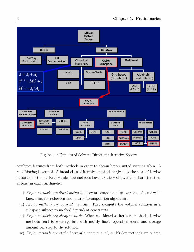
them. Figures 1.1 and 1.2 show these three groups of methods and its sub-groups. Even
though the computation of eigenvalues has to be iterative, previous reductions to simpler
form are mostly based on direct approaches. Direct approaches are more natural and have
been used for a long time. Most direct methods used nowadays are stable and robust.
Large scale matrix computations are often based on iterative approaches. The overlap-
ping and non-overlapping Domain Decomposition Methods is an hybrid technique that
3
4 Chapter 1. Preliminaries
Figure 1.1: Families of Solvers: Direct and Iterative Solvers
combines features from both methods in order to obtain better suited systems when ill-
conditioning is verified. A broad class of iterative methods is given by the class of Krylov
subspace methods. Krylov subspace methods have a variety of favorable characteristics,
at least in exact arithmetic:
i) Krylov methods are direct methods. They are coordinate free variants of some well-
known matrix reduction and matrix decomposition algorithms.
ii) Krylov methods are optimal methods. They compute the optimal solution in a
subspace subject to method dependent constraints.
iii) Krylov methods are cheap methods. When considered as iterative methods, Krylov
methods tend to converge fast with mostly linear operation count and storage
amount per step to the solution.
iv) Krylov methods are at the heart of numerical analysis. Krylov methods are related

5
Additive Schwarz Methods Multiplicative Schwarz Methods
Overlapping DDM
Domain Decomposition Methods (Preconditioners)
non−Overlapping DDM
Schur Complement Matrix prec.(Substructuring)
Neumann−Neumann prec.
FETI (and its variants)
Block−Jacobi prec.
Coarse correction variants
Present Research Proposal
Balancing Neumann−Neumann prec.
Figure 1.2: Families of Solvers: Domain Decomposition Solvers
Figure 1.3: Aleksei Nikolaevich Krylov (1863–1945)
to structured eigenvalue problems, to orthogonal polynomials, to rational approxi-
mation theory. Amongst others, this enables detailed convergence analysis.

6 Chapter 1. Preliminaries
v) Krylov methods are closely related to each other. In particular, a linear system solver
can be used to extract eigenvalues, and vice versa.
On the other hand, in finite precision arithmetic (an original work on this topic can be
consulted in Reference [Zem03]), Krylov methods do not terminate after a finite number
of steps. The solutions are not optimal in the Krylov subspace constructed. Nevertheless,
Krylov methods compute useful results. Only a part of the matrix relations defining the
methods in infinite precision have a finite precision counterpart.
A numerical analysis sight shows an important difference between dense and sparse
systems. For dense systems the state of the art almost seems to have reached its final
destination via a variety of well-known and well understood algorithms. The situation
is not optimistic when looking at sparse systems. Most direct methods lead to storage
problems due to fill-in and numerical instabilities due to restrictions on the pivoting
strategies. The classical iterative methods like Jacobi, Gauß-Seidel and SOR in general
are converging too slowly to the solution to be of practical use. Krylov subspace methods
Figure 1.4: Carl Gustav Jacob Jacobi (1804–1851)
are direct methods (they terminate after a finite number of steps, at least in theory) and
improve over the classical iterative methods in the sense of being optimal. Krylov methods
are frequently the method of choice for large sparse problems. Past Krylov methods were
developed in the early fifties and the first papers written by Lanczos also appeared by
that years [Lan50, Arn51]. Due to a lack of better understanding (i.e., the methods
where not competitive to the other direct methods in terms of accuracy and stability)
they were abandoned, or only used in conjunction with complete reorthogonalization,
which made them less competitive. It was necessary almost twenty years for theoretical
and practical recognition of Krylov methods. Krylov methods are only competitive when

1.1. Solution of Linear Systems 7
Figure 1.5: Johann Carl Friedrich Gauß (1777–1855)
used with preconditioning. There is a vast amount of work in scientific journals such
as Mathematics of Computation, SIAM Journal on Matrix Analysis and Applications,
SIAM Journal on Numerical Analysis, Computer Methods in Applied Mechanics and
Engineering, International Journal for Numerical Methods in Engineering, Journal of
Computational Physics about preconditioning techniques and the application on solving
continuum mechanics problems (most of them are references along this thesis). Though,
Domain Decomposition Methods and its variants are treated as Preconditioner for General
Krylov Methods like Conjugate Gradients and/or Generalized Minimal Residuals. Part
of this thesis is focused on this topic.
1.1 Solution of Linear Systems
The linear system under consideration will be denoted in this section as Ax = b, where
we assume that A ∈ Kn×n and b ∈ Kn are known and we look for a solution x ∈ Kn.
This solution is unique when A is regular. For regular A, the entries xi of the solution x
depend analytically on the entries of A and b. This is known as Cramer’s rule
xi =det(a1, ..., ai−1, b, ai+1, ..., an)
det(A). (1.1)
This relation is merely of theoretical interest.
1.1.1 Perturbation Theory
The linear system and the related perturbed system will be denoted by Ax = b and
Ax = b, respectively. We suppose that A ∈ Kn×n and b ∈ Kn are given, and we seek

8 Chapter 1. Preliminaries
x ∈ Kn. Also, we define the differences
∆A = A− A, ∆x = x− x and b = b− b. (1.2)
We interpret x as an approximate solution of Ax = b and denote the corresponding
residual by r = b− Ax.
1.1.2 Condition Number
A condition number is a bound on the set of changes computed using perturbation theory.
A variety of useful condition numbers can be defined. We can define the norm-wise
condition number of the system Ax = b as
κα,β(A, x) ≡ infε>0
sup
||∆x||||x||
ε : Ax = b, ∆A ≤ εα, ∆b ≤ εβ
(1.3)
=||A−1||(α||x||+ β)
||x||, (1.4)
for the particular choice of α = ||A|| and β = ||b||. Generally, for a non-singular matrix
A, the norm-wise condition number can be written as
κ(A) = ||A||||A−1||, (1.5)
or simply
κ(A) = λmax(A)/λmin(A) (1.6)
if the matrix is symmetric and positive definite. The simbol ‖.‖ denotes any suitable
norm.
When the condition number is small, backward stable algorithms are also forward
stable. A problem is termed ill-conditioned when the condition number is large, and
ill-posed when the condition number is infinite. Ill-posed problems can not be solved in
finite precision.
1.2 Preconditioning
The main objective of preconditioning techniques is the lowering of the condition number
for ill-conditioned systems. That is why frequently domain decomposition methods are
considered preconditioners instead of solvers. Nevertheless, it is imperative the use of some
preconditioning in some domain decomposition schemes. This topic will be discussed in §2.
Another important issue of preconditioning is the improvement of the spectral properties
(i.e., the eigenvalues distribution) of the preconditioned system.

1.3. Basic Iterative Method 9
Basically, preconditioning consists in multiplying (on the left or right side of matrix
A and vector b) both side of the original system by a matrix P (i.e., the ‘preconditioner’)
such that
PAx = Pb, (1.7)
and such that κ(PA) κ(A) and the eigenvalues are grouped in clusters. In other words,
matrix PA has better invertible properties than original matrix A.
There exist a wide variety of preconditioning techniques. Some preconditioners are
based on straight insight of the structure of the problem at hand. Other preconditioners,
which in general depend on the topology where the problems are defined, are multigrid
and domain decomposition methods, alternating direction preconditioners. Nevertheless,
there exist fully algebraic versions of such preconditioners/solvers. One commonly used
and easy to implement preconditioner is Jacobi preconditioning, where P is the inverse
of the diagonal part of A. One can also use other preconditioners based on the classical
stationary iterative methods, such as the symmetric Gauß–Seidel preconditioner. For
applications to PDE’s, these preconditioners have no very effective performances. Another
approach is to apply a sparse Cholesky factorization to the matrix A (thereby giving up a
fully matrix-free formulation) and discarding small elements of the factors and/or allowing
only a fixed amount of storage for the factors. Such preconditioners are called incomplete
factorization preconditioners. One could also attempt to estimate the spectrum of A, find
a polynomial p such that 1−zp(z) is small on the approximate spectrum, and use p(A) as
a preconditioner. This is the so-called polynomial preconditioning. The preconditioned
system is
p(A)Ax = p(A)b, (1.8)
and one would expect the spectrum of p(A)A to be more clustered near z = 1 than
that of A. If an interval containing the spectrum can be found, the residual polynomial
q(z) = 1−zp(z) of smallest L∞ norm on that interval can be expressed in terms of Cheby-
shev polynomials. Alternatively q can be selected to solve a least squares minimization
problem.
1.3 Basic Iterative Method
A basic algorithm that leads to many effective iterative solvers, is to split the matrix of a
given linear system into a sum of two matrices, one of which leads to a system well suited
to solve. The most simple splitting we can think of is A = I − (I − A). This splitting

10 Chapter 1. Preliminaries
Figure 1.6: Andre-Louis Cholesky (1875–1918)
Figure 1.7: Pafnuty Lvovich Chebyshev (1821–1894)
leads to the well-known Richardson iteration for the linear system:
xi+1 = (I − A)xi + b = xi + ri. (1.9)
Multiplying by −A and adding b gives
−Axi+1 + b = −Axi − Ari + b, (1.10)
and
ri+1 = (I − A)ri = (I − A)i+1r0 = Pi+1(A)r0, (1.11)
or, in terms of the error
A(x− xi+1) = Pi+1(A)A(x− x0), (1.12)

1.3. Basic Iterative Method 11
then
x− xi+1 = Pi+1(A)(x− x0). (1.13)
In last equations Pi+1 is a polynomial of degree i + 1. Note that Pi+1(0) = 1. A more
Figure 1.8: Lewis Fry Richardson (1881–1953)
general splitting A = M −N = M − (M −A) can be rewritten as the standard splitting
B = I − (I −B) for the preconditioned matrix B = M−1A = PA.
Now, assume that x0 = 0 without loss of generality. Thus, the simple Richardson
iteration is such that
xi+1 = r0 + r1 + r2 + ...+ ri =i∑
j=0
(I − A)jr0, (1.14)
and xi ∈ r0, r1, ..., ri ≡ r0, Ar0, ..., Air0 = Ki+1(A; r0), being Ki+1(A; r0) the Krylov
subspace associated to A and r0 (and i.e., b).
1.3.1 Optimal Iteration Methods
A difficulty associated with classical/stationary iterative methods (e.g., SOR, Chebychev
semi-iterative, etc.) is that they depend upon some parameters that are sometimes hard
to choose in proper manner. The natural question is how to get good approximations
xi+1 from the Krylov subspace that is generated by the basic iterative method. A good
choose seems to be those xi+1 for which ||xi+1 − x|| (for a well suited norm) is minimal.
In general (see [Kel95]), an optimal choose on the search direction is such that ||xi− x||Ais minimal for xi ∈ Ki(A; r0). That is
xi − x ⊥A Ki(A; r0) (1.15)

12 Chapter 1. Preliminaries
or
ri ⊥ Ki(A; r0), (1.16)
for the ‘energy’ norm ||.||A.
Using Lanczos’s iteration, the Conjugate Gradients method proposed by Hestener and
Stiefel in [HS52] and the Generalized Minimal Residuals method by Saad and Schultz [SS86]
for symmetric positive definite matrices and non-singular diagonalizable matrices, respec-
tively, exploit the considerations expressed above. These kind of methods will be used in
Figure 1.9: Cornelius Lanczos (1893–1974)
this thesis in the context of Domain Decomposition techniques.

Chapter 2
The ‘Interface Strip Preconditioner’
for Domain Decomposition Methods
Find a job you love
and you’ll never work a day in your life.
Kong Fuzi (Confucius)
In this chapter, a new preconditioner for iterative solution of the interface problem in
Schur Complement Domain Decomposition Methods is presented. Also, the efficiency of
this parallelizable preconditioner is studied in the context of the solution of non-symmetric
linear equations arising from discretization of the Partial Differential Equations. The
proposed Interface Strip Preconditioner (ISP) is based on solving a global problem in a
narrow strip around the interface. It requires much less memory and computing time
than classical Neumann-Neumann preconditioner, and handles correctly the flux splitting
among sub-domains that share the interface. The performance of this preconditioner is
assessed with an analytical study of Schur complement matrix eigenvalues and numerical
experiments conducted in parallel computational environment (consisting of a Beowulf
cluster of twenty nodes).
The aim of this chapter is to present a theoretical basis (regarding the behavior of
Schur complement matrix spectra) and some simple and complex numerical experiments
13
14Chapter 2. The ‘Interface Strip Preconditioner’ for Domain Decomposition
Methods
conducted in sequential and parallel platforms as a motivation for adopting the proposed
preconditioner. Efficiency, scalability, and implementation details on a production parallel
finite element code [SYNS02, SNPD06] will be presented in the next chapter (also, see
References [PS05, PNS06]).
2.1 Introduction
The large spread in length scales present in CFD problems (like viscous/inviscid com-
pressible/incompressible flows around bodies, river/aquifer interactions, open channels,
etc.) requires a high degree of refinement in the finite element mesh and, then, requires
very large computational resources. It is known that the number of grid points in a 3D
mesh for a turbulence DNS model grows with the Reynolds number as <9/4. Also, in a
2D coupled surface-subsurface flow problem, a typical multi-aquifer model, the number of
unknowns per surface node is, at least, equal to the number of aquifers and aquitards. Due
to this fact, it is expected to have a very high demand of CPU computation time, calling
for parallel processing techniques. Linear systems obtained from discretization of PDE’s
by means of Finite Difference or Finite Element Methods are normally solved in paral-
lel by iterative methods [Saa00, Meu99] because they require much less communication
compared to direct solvers.
The Schur complement domain decomposition method leads to a reduced system better
suited for iterative solution than the global system, since its condition number is lower
(∝ 1/h vs ∝ 1/h2 for the global system, h being the mesh size) and the computational
cost per iteration is not so high once the sub-domain matrices have been factorized.
Iterative substructuring methods rely on a non-overlapping partition into sub-domains
(substructures). The efficiency of these methods can be further improved by using pre-
conditioners [LTV97]. Once the degrees of freedom inside the substructures have been
eliminated by block Gaussian elimination (or other algorithm), a preconditioner for the
resulting Schur complement system is built with matrix blocks relative to a decompo-
sition of interface finite element functions into subspaces related to geometrical objects
(vertices, edges, faces, single substructures) or simply by the coefficients of sub-domain
matrices near the interface. Iterative methods like Conjugate Gradients and GMRes are
then employed. Early works, such as [BPS86, BPS89], have influenced most of the later
work in the field. They proposed two spaces for the coarse problem. One of their coarse
spaces is given in terms of the averages of the nodal values over the entire substructure
boundaries ∂Ωi. The other space is defined by extending the wire basket (recall that the
wire basket is the union of the boundaries of the faces that separate the substructures)

2.1. Introduction 15
values as a two dimensional discrete harmonic function onto the faces, and then as a
discrete harmonic function into the interiors of the sub-domains. For self-adjoint posi-
Figure 2.1: Issai Schur (1875–1941)
Figure 2.2: Carl Gottfried Neumann (1832–1925)
tive semidefinite problems, Neumann-Neumann preconditioner is the most classical one.
From a mathematical point of view, the preconditioner is defined by approximating the
inverse of the global Schur complement matrix by the weighted sum of local Schur com-
plement matrices. From a physical point of view, Neumann-Neumann preconditioner is
based on splitting the flux applied to the interface in the preconditioning step and solving
local Neumann problems in each sub-domain. This strategy is good only for symmetric
operators.
The preconditioner proposed here is based on solving a problem in a ‘strip’ of nodes
around the interface (see Figure 2.3). When the width of the strip is narrow, the com-
putational cost and memory requirements are low and the iteration count is relatively

16Chapter 2. The ‘Interface Strip Preconditioner’ for Domain Decomposition
Methods
high, when the strip is wide, the converse is verified. This preconditioner performs better
(I)Strip
21
interface stripnodes in the
interior nodes
ΩΩ
Interface
Figure 2.3: Domain Decomposition
for non-symmetric operators and does not have rigid body modes for internal floating
sub-domains, as is the case for the Neumann-Neumann preconditioner. Recall that for
operators that involve only derivatives of the unknowns (as Laplace equation, steady
elasticity, steady advection-diffusion, for instance) a portion of the boundary should have
Dirichlet or mixed boundary conditions. Otherwise, the problem is ill-posed and the
matrix is singular. When using the Neumann-Neumann preconditioner, sub-domains in-
herit the boundary condition of the original problem in the external boundary, whereas
Neumann boundary conditions are imposed at the internal sub-domain interfaces. Sub-
domains that have a non-empty intersection with a portion of the Dirichlet part of the
external boundary do not have rigid modes. Sub-domains whose boundary has empty
intersection with the external Dirichlet or mixed portion of the boundary would have
Neumann condition imposed on their whole boundary and would have rigid modes for
the kind of operators described above. In contrast with the wire-basket algorithms, the
IS preconditioner is purely algebraic, i.e., it can be assembled from a subset of the matrix
coefficients. There are no requirements on the topology of the mesh, and even it could
be applied to sparse matrices coming from other kind of problems, not necessarily from
PDE discretizations.
Linear systems obtained from discretization of PDE’s by means of FDM or FEM
are normally solved in parallel by iterative methods [Saa00] because they are much less
coupled than direct solvers.
2.1. Introduction 17
Figure 2.4: Johann Peter Gustav Lejeune Dirichlet (1805–1859)
The Schur complement domain decomposition method leads to a reduced system better
suited for iterative solution than the global system, since its condition number is lower
(∝ 1/h vs ∝ 1/h2 for the global system, h being the mesh size) and the computational cost
per iteration is not so high once the sub-domain matrices have been factorized. In addition,
it has other advantages over global iteration. It solves bad ‘inter-equation’ conditioning,
it can handle Lagrange multipliers and in a sense it can be thought as a mixture between
a global direct solver and a global iterative one. The efficiency of iterative methods
Figure 2.5: Joseph–Louis Lagrange (1736–1813)
can be further improved by using preconditioners [LTV97]. For mechanical problems,
Neumann-Neumann is the most classical one. From a mathematical point of view, the
preconditioner is defined by approximating the inverse of the global Schur complement
matrix by the weighted sum of local Schur complement matrices. From a physical point
of view, Neumann-Neumann preconditioner is based on splitting the flux applied to the

18Chapter 2. The ‘Interface Strip Preconditioner’ for Domain Decomposition
Methods
interface in the preconditioning step and solving local Neumann problems in each sub-
domain. This strategy is good only for symmetric operators.
A new preconditioner based on solving a global problem in a strip of nodes around the
interface is proposed. A similar idea has been already exploited in the context of FETI
methods [RMSB03] in order to construct an approximation of local Schur complement
matrices. In contrast, the preconditioning technique considered here approximates the
inverse of global Schur matrix. This preconditioner performs better for non-symmetric
operators; it does not suffer from the rigid body modes for internal floating sub-domains
as is the case for the Neumann-Neumann preconditioner and naturally conducts to sub-
domain coupling (thus eliminating the need of a coarse problem). A detailed computation
of the eigenvalue spectra for simple cases and some numerical examples are presented.
2.2 Schur Complement Domain Decomposition Me-
thod
Consider solving in each time step a linearized form of system (i.e., Au = f) resulting
from finite element discretization as described in the next sections. Let Ω denote the
computational domain of the CFD problem, and Ωii=ni=1 its decomposition into n non-
overlapping sub-domains. Now, reorder u and f as u = (uL, uI)T and f = (fL, fI)
T ,
numbering the global nodes such that the coefficient matrices of variables assume block-
ordered structure
A =
[ALL ALI
AIL AII
], (2.1)
where ALL = diag[A11,A22, ...,ANsNs ] is a block-diagonal with each block Aii, i =
1, 2, ..., Ns being the matrix corresponding to the unknowns belonging to the interior ver-
tices of sub-domain Ωi. Blocks ALI and AIL represents connections between sub-domains
to interfaces.
Block AII corresponds to the discretization of the differential operator restricted to
the interfaces and represents the coupling between local interface points.
The numerical solution of Au = f is equivalent to solving
SuI = g on interfaces Γ, (2.2)
and
ALLuL = fL −ALIuI in Ωi, (2.3)

2.2. Schur Complement Domain Decomposition Method 19
being
S = AII −Ns∑i=1
AILA−1LLALI , (2.4)
and
g = fI −Ns∑i=1
AILA−1LLfL, (2.5)
where S is the well-known Schur complement matrix. If Si is the Schur Complement
matrix associated to the i-subdomain, then equations (2.4) and (2.5) can be written as
Si = AiII −Ai
ILAi−1LL Ai
LI , (2.6)
and
gi = f iI −Ai
ILAi−1LL f
iL. (2.7)
Also, if the restriction operator Ri, which extracts from a global vector u the entries
corresponding to the interface nodes such that uI = Riu, is introduced then
S =Ns∑i=1
RTi SiRi (2.8)
and
g = fI −Ns∑i=1
RTi Ai
ILAi−1LL f
iL. (2.9)
The Schur domain decomposition method starts by first determining uI on the interfaces
between sub-domains by solving (2.2). Upon obtaining uI , the sub-domain problems (2.3)
decouple and may be solved in parallel. The main computational cost for the iterative
solution of (2.2) depends on the number of iteration, i.e., the condition number, to achieve
convergence to a given accuracy criterion.
It is clear that the knowledge of the eigenvalue spectrum of the Schur complement
matrix is one of the most important issues in order to develop suitable preconditioners.
To obtain analytical expressions for Schur complement matrix eigenvalues and also the
influence of several preconditioners, a simplified problem is considered, namely the solution
to the Poisson problem in a unit square
∆φ = g, in Ω = 0 < x, y < 1, (2.10)
with boundary conditions
φ = φ, at Γ = x, y = 0, 1, (2.11)

20Chapter 2. The ‘Interface Strip Preconditioner’ for Domain Decomposition
Methods
Figure 2.6: Simon-Denis Poisson (1781–1840)
where φ is the unknown, g(x, y) is a given source term and Γ is the boundary. Consider
now the partition of Ω in Ns non-overlapping sub-domains Ω1, Ω2, . . . ,ΩNs , such that
Ω = Ω1
⋃Ω2
⋃. . .⋃
ΩNs . For the sake of simplicity, let assume that the sub-domains
are rectangles of unit height and width Lj. In practice this is not the best partition,
but it will allow us to compute the eigenvalues of the interface problem in closed form.
Let Γint = Γ1
⋃Γ2
⋃. . .⋃
ΓNs−1 be the interior interfaces among adjacent sub-domains.
Given a guess ψj for the trace of φ in the interior sub-domains φ|Γj, each interior problem
can be solved independently as
∆φ = g, in Ωj,
φ =
ψj−1, at Γj−1,
ψj, at Γj,
φ, at Γup,j + Γdown,j,
(2.12)
where ψ0 = φ∣∣x=0
and ψNs = φ∣∣x=1
are given.
2.2.1 The Steklov Operator
Not all combinations of trace values ψj give the solution of the original problem (2.10).
Indeed, the solution to (2.10) is obtained when the trace values are chosen in such a way
that the flux balance condition at the internal interfaces is satisfied,
fj =∂φ
∂x
∣∣∣∣−Γj
− ∂φ
∂x
∣∣∣∣+Γj
= 0, (2.13)
where the ± superscripts stand for the derivative taken from the left and right sides of
the interface. We can think of the correspondence between the ensemble of interface
2.2. Schur Complement Domain Decomposition Method 21
values ψ = ψ1, . . . , ψNs−1 and the ensemble of flux imbalances f = f1, . . . , fNs−1 as
an interface operator S such that
Sψ = f − f0, (2.14)
where all inhomogeneities coming from the source term and Dirichlet boundary conditions
are concentrated in the constant term f0, and the homogeneous operator S is equivalent
to solving the equation set (2.12) with source term g = 0 and homogeneous Dirichlet
boundary conditions φ = 0 at the external boundary Γ. Here, S is the Steklov operator.
Figure 2.7: Vladimir Andreevich Steklov (1864–1926)
In a more general setting, it relates the unknown values and fluxes at boundaries when the
internal domain is in equilibrium. In the case of internal boundaries, it can be generalized
by replacing the fluxes by the flux imbalances. The Schur complement matrix is a discrete
version of the Steklov operator, and we will show that in this simplified case we can
compute the Steklov operator eigenvalues in closed form, and then a good estimate for
the corresponding Schur complement matrix ones.
2.2.2 Eigenvalues of Steklov Operator
We will further assume that only two sub-domains are present, one of them at the left
of width L1 and the other at the right of width L2, so that L = L1 + L2 = 1 is the side
length.
We solve first the Laplace problem in each sub-domain with homogeneous Dirichlet

22Chapter 2. The ‘Interface Strip Preconditioner’ for Domain Decomposition
Methods
boundary condition at the external boundary and ψ at the interface,
∆φ = 0, in Ω1,2,
φ =
0, at Γ,
ψ, at Γ1.
(2.15)
The solution of (2.15) can be expressed as a linear combination of functions of the form
Figure 2.8: Pierre–Simon Laplace 1749–1827)
φn(x, y) =
[sinh(knx)/ sinh(knL1)] sin(kny), 0 ≤ x ≤ L1,
[sinh(kn(L− x))/ sinh(knL2)] sin(kny), L1 ≤ x ≤ L,(2.16)
where the wave number kn and the wavelength λn are defined as
kn = 2π/λn, λn = 2L/n, n = 1, . . . ,∞. (2.17)
The flux imbalance for each function in (2.16) can be computed as
fn =∂φn
∂x
∣∣∣∣x=L−1
− ∂φn
∂x
∣∣∣∣x=L+
1
=
= kn
(cosh(knL1)
sinh(knL1)+
cosh(knL2)
sinh(knL2)
)sin(kny) =
= kn [coth(knL1) + coth(knL2)] sin(kny).
(2.18)
A given interface value function ψ is an eigenfunction of the Steklov operator if the
corresponding flux imbalance f = Sψ is proportional to ψ, i.e., Sψ = ωψ, ω being the
2.2. Schur Complement Domain Decomposition Method 23
corresponding eigenvalue. We can see from (2.15) to (2.18) that the eigenfunctions of the
Steklov operator are
ψn(y) = sin(kny) (2.19)
with eigenvalues
ωn = eig(S)n = eig(S−)n + eig(S+)n =
= kn [coth(knL1) + coth(knL2)] ,(2.20)
where S∓ are the Steklov operators of the left and right sub-domains,
S∓ψ = ± ∂φ
∂x
∣∣∣∣L∓1
, (2.21)
and their eigenvalues are
eig(S∓)n = kn coth(knL1,2). (2.22)
For large n, the hyperbolic cotangents in (2.22) both tend to unity. This shows that
the eigenvalues of the Steklov operator grow proportionally to n for large n, and then
its condition number is infinity. However, when considering the discrete case the wave
number kn is limited by the largest frequency that can be represented by the mesh, which
is kmax = π/h where h is the mesh spacing. The maximum eigenvalue is
ωmax = 2kmax =2π
h, (2.23)
which grows proportionally to 1/h. As the lowest eigenvalue is independent of h, this
means that the condition number of the Schur complement matrix grows as 1/h. Note
that the condition number of the discrete Laplace operator typically grows as 1/h2. Of
course, this reduction in the condition number is not directly translated to total compu-
tation time, since we have to take account of the factorization of the sub-domain matrices
and forward and backward substitutions involved in each iteration to solve internal prob-
lems. However, the overall balance is positive and reduction in the condition number,
besides being inherently parallel, turns out to be one of the main strengths of domain
decomposition methods.
In Figure 2.9 we can see the first and tenth eigenfunctions computed directly from the
Schur complement matrix for a 2 sub-domain partition, whereas in Figure 2.10 we see
the first and twenty-fourth eigenfunction for a 9 sub-domain partition. The eigenvalue
magnitude is related to eigenfunction frequency along the inter-subdomain interface, and
the penetration of the eigenfunctions towards sub-domains interiors decays strongly for
higher modes∗.
∗I would like to thank to Lisandro Dalcın for the confection of Figures 2.9 and 2.10

24Chapter 2. The ‘Interface Strip Preconditioner’ for Domain Decomposition
Methods
(a) 1st eigenfunction
(b) 10th eigenfunction
Figure 2.9: Eigenfunctions of Schur complement matrix with 2 sub-domains
2.3 Preconditioners for the Schur Complement Ma-
trix
In order to further improve the efficiency of iterative methods, a preconditioner has to
be added so that the condition number of the Schur complement matrix is lowered. The
most known preconditioners for mechanical problems are Neumann-Neumann and its
variants [Man93, Cro02, BR96] for Schur complements methods, and Dirichlet for FETI

2.3. Preconditioners for the Schur Complement Matrix 25
(a) 1st eigenfunction
(b) 10th eigenfunction
Figure 2.10: Eigenfunctions of Schur complement matrix with 9 sub-domains
methods and its variants [FR91, FMR94, FM98, FLLT+01, RMSB03]. It can be proved
that they reduce the condition number of the preconditioned operator to O(1) (i.e., inde-
pendent of h) in some special cases.
2.3.1 The Neumann-Neumann Preconditioner
Consider the Neumann-Neumann preconditioner
PNNv = f, (2.24)
where
v(y) = 1/2[v1(L1, y) + v2(L1, y)], (2.25)

26Chapter 2. The ‘Interface Strip Preconditioner’ for Domain Decomposition
Methods
and vi, i = 1, 2, are defined through the following problems
∆vi = 0 in Ωi,
vi = 0 at Γ0 + Γup,i + Γdown,i,
(−1)i−1∂vi
∂x= 1/2f at Γ1.
(2.26)
The preconditioner consists in assuming that the flux imbalance f is applied on the
interface. Since the operator is symmetric and the domain properties are homogeneous,
this ‘load’ is equally split among the two sub-domains. Then, we have a problem in
each sub-domain with the same boundary conditions in the exterior boundaries, and a
non-homogeneous Neumann boundary condition at the inter-subdomain interface.
Again, we will show that the eigenfunctions of the Neumann-Neumann preconditioner
are (2.19). Effectively, we can propose for v1 the form
v1 = C sinh(knx) sin(kny), (2.27)
where C is determined from the boundary condition at the interface in (2.26) and results
in
C =1
2kn cosh(knL1), (2.28)
and similarly for v2, so that
v1(x, y) =1
2kn
sinh(knx)
cosh(knL1)sin(kny),
v2(x, y) =1
2kn
sinh(kn(L− x))
cosh(knL2)sin(kny).
(2.29)
Then, the value of v = P−1NNf can be obtained from (2.25)
v(y) = P−1NNf =
1
4kn
[tanh(knL1) + tanh(knL2)] sin(kny), (2.30)
so that the eigenvalues of PNN are
eig(PNN)n = 4kn [tanh(knL1) + tanh(knL2)]−1 . (2.31)
As its definition suggests, it can be verified that
eig(PNN)n = 4 [eig(S−)−1n + eig(S+)−1
n ]−1. (2.32)
As the Neumann-Neumann preconditioner (2.24) and the Steklov operator (2.14) diago-
nalize in the same basis (2.19) (i.e., they ‘commute’ ), the eigenvalues of the preconditioned
operator are simply the quotients of the respective eigenvalues, i.e.,
eig(P−1NNS)n = 1/4[tanh(knL1) + tanh(knL2)] [coth(knL1) + coth(knL2)]. (2.33)

2.3. Preconditioners for the Schur Complement Matrix 27
We see that all tanh(knLj) and coth(knLj) factors tend to unity for n→∞, then we have
eig(P−1NNS)n → 1 for n→∞, (2.34)
so that this means that the preconditioned operator P−1NNS has a condition number O(1),
i.e., it doesn’t degrade with mesh refinement. This is optimal, and is a well known feature
of the Neumann-Neumann preconditioner. In fact, for a symmetric decomposition of the
domain (i.e., L1 = L2 = 1/2), we have
eig(P−1NNS)n =
1
42 tanh(kn/2) 2 coth(kn/2) = 1, (2.35)
so that the preconditioner is equal to the operator and convergence is achieved in one
iteration.
Note that comparing (2.20) and (2.32) we can see that the preconditioning is effective
as long as
eig(S−)n ≈ eig(S+)n. (2.36)
This is true for symmetric operators and symmetric domain partitions (i.e., L1 ≈ L2).
Even for L1 6= L2, if the operator is symmetric, then (2.36) is valid for large eigenvalues.
However, this fails for non-symmetric operators as in the advection-diffusion case, and
also for irregular interfaces.
Another aspect of the Neumann-Neumann preconditioner is the occurrence of indef-
inite internal Neumann problems, which leads to the need of solving a coarse prob-
lem [Man93, Cro02] in order to solve the ‘rigid body modes’ for internal floating sub-
domains. The coarse problem couples the sub-domains and hence ensures scalability
when the number of sub-domains increases. However, this adds to the computational cost
of the preconditioner.
2.3.2 The Interface Strip Preconditioner (ISP)
A key point about the Steklov operator is that its high frequency eigenfunctions decay
very strongly far from the interface, so that a preconditioning that represents correctly the
high frequency modes can be constructed if we solve a problem on a narrow strip around
the interface. In fact, the n-th eigenfunction with wave number kn given by (2.16) decays
far from the interface as exp(−kn|s|) where s is the distance to the interface. Then, these
high frequency modes will be correctly represented if we solve a problem on a strip of
width b around the interface, provided that the interface width is large with respect to
the mode wave length λn.

28Chapter 2. The ‘Interface Strip Preconditioner’ for Domain Decomposition
Methods
The ‘Interface Strip Preconditioner’ (ISP) is defined as
PISv = f, (2.37)
where
f =∂w
∂x
∣∣∣∣x=L−1
− ∂w
∂x
∣∣∣∣x=L+
1
(2.38)
and∆w = 0 in 0 < |x− L1| < b and 0 ≤ x ≤ 1,
w = 0 at |x− L1| = b or y = 0, 1,
w = v at x = L1.
(2.39)
Please note that for high frequencies (i.e., knb large) the eigenfunctions of the Steklov
operator are negligible at the border of the strip, so that the boundary condition at
|x − L1| = b is justified. The eigenfunctions for this preconditioner are again given
by (2.19) and the eigenvalues can be taken from (2.20), replacing L1,2 by b, i.e.,
eig(PIS)n = 2 eig(Sb)n = 2kn coth(knb), (2.40)
where Sb is the Steklov operator corresponding to a strip of width b.
For the preconditioned Steklov operator, we have
eig(P−1IS S)n = 1/2 tanh(knb) [coth(knL1) + coth(knL2)] . (2.41)
Note that eig(P−1IS S)n → 1 for n→∞, so that the preconditioner is optimal, independently
of b. Also, for b large enough we recover the original problem so that the preconditioner is
exact (convergence is achieved in one iteration). However, in this case the use of this pre-
conditioner is impractical, since it implies solving the whole problem. Note that in order
to solve the problem for v information from both sides of the interface is needed, while
the Neumann-Neumann preconditioner can be solved independently in each sub-domain.
This is a disadvantage in terms of efficiency, since we have to waste communication time
in sending the matrix coefficients in the strip from one side to the other or otherwise
compute them in both processors. However, we will see that efficient preconditioning can
be achieved with few node layers and negligible communication. Moreover, we can solve
the preconditioner problem by iteration, so that no migration of coefficients is needed.
2.4 The Advective-Diffusive Case
Consider now the advective diffusive case,
κ∆φ− uφ,x = g in Ω, (2.42)

2.4. The Advective-Diffusive Case 29
where κ is the thermal conductivity of the medium and u the advection velocity. The
problem can be treated in a similar way, and the Steklov operators are defined as
S∓ψ = ± φ,x|L∓1 , (2.43)
whereκ∆φ− uφ,x = 0 in Ω1,2,
φ =
0 at Γ,
ψ at Γ1.
(2.44)
The eigenfunctions are still given by (2.19). Looking for solutions of the form v ∝exp(µx) sin(kny) we obtain a constant coefficient second order differential equation with
characteristic polynomial
κµ2 − uµ− κk2n = 0, (2.45)
whose roots are
µ± =u±
√u2 + 4κ2k2
n
2κ=
u
2κ± δn. (2.46)
After some algebra, the solution of (2.44) is
φn =
eu(x−L1)/2κ sinh(δnx)sinh(δL1)
sin(kny) for 0 ≤ x ≤ L1, 0 ≤ y ≤ L,
eu(x−L1)/2κ sinh(δn(L−x))sinh(δL2)
sin(kny) for L1 ≤ x ≤ L, 0 ≤ y ≤ L,(2.47)
and the eigenvalues are then
eig(S−)n =u
2κ+ δn coth(δnL1)
eig(S+)n = − u
2κ+ δn coth(δnL2).
(2.48)
In Figure 2.11 we see the first and tenth eigenfunctions for a problem with an advection
term at a global Peclet number of Pe = uL/2κ = 2.5. For low frequency modes, advective
effects are more pronounced and the first eigenfunction (on the left) is notably biased
to the right. In contrast, for high frequency modes (like the tenth mode shown at the
right) the diffusive term prevails and the eigenfunction is more symmetric about the
interface, and (as in the pure diffusive case) concentrated around it. Note that now the
eigenvalues for the right and left part of the Steklov operator may be very different due
to the asymmetry introduced by the advective term. This difference in splitting is more
important for the lowest mode. In Figures 2.12 to 2.15 we see the eigenvalues as a function
of the wave number kn. Note that for a given side length L only a certain sequence of
wave numbers, given by (2.17) should be considered. However, it is perhaps easier to
consider the continuous dependence of the different eigenvalues upon the wave number k.

30Chapter 2. The ‘Interface Strip Preconditioner’ for Domain Decomposition
Methods
(a) 1st eigenfunction
(b) 10th eigenfunction
Figure 2.11: Eigenfunctions of Schur complement matrix with 2 sub-domains and advec-
tion (global Peclet 5)
For a symmetric operator and a symmetric partition (see Figure 2.12), the symmetric
flux splitting is exact and the Neumann-Neumann preconditioner is optimal. The largest
discrepancies between the ISP preconditioner and the Steklov operator occur at low fre-
quencies and yield a condition number less than two. If the partition is non-symmetric
(see Figure 2.13) then the Neumann-Neumann preconditioner is no longer exact, because
S+ 6= S−. However, its condition number is very low whereas the IS preconditioner con-
dition number is still under two. For a relatively important advection term, given by a

2.4. The Advective-Diffusive Case 31
! #"$&%'
() *+,-.-'/01 23465 798
:
;<= >@?
ACBED
Figure 2.12: Eigenvalues of Steklov operators and preconditioners for the Laplace operator
(Pe = 0) and symmetric partitions (L1 = L2 = L/2, b = 0.1L)

32Chapter 2. The ‘Interface Strip Preconditioner’ for Domain Decomposition
Methods
"!#$ %&'()
*,+ -.0/1
2
34 56798 :<;
=>9?@A
BCED
Figure 2.13: Eigenvalues of Steklov operators and preconditioners for the Laplace operator
(Pe = 0) and non-symmetric partitions (L1 = 0.75L, L2 = 0.25L, b = 0.1L)

2.4. The Advective-Diffusive Case 33
global Peclet number of 5 (see Figure 2.14), the asymmetry in the flux splitting is much
more evident, mainly for small wave numbers, and this results in a large discrepancy
between the Neumann-Neumann preconditioner and the Steklov operator. On the other
hand, the IS preconditioner is still very close to the Steklov operator. The difference
between the Neumann-Neumann preconditioner and the Steklov operator increases for
larger Pe (see Figure 2.15). This behavior can be directly verified by computing the con-
dition number of Schur complement matrix and preconditioned Schur complement matrix
for the different preconditioners (see Tables 2.1 and 2.2). We can see that, for low Pe, both
the Neumann-Neumann and ISP preconditioners give a similar preconditioned condition
number regardless of mesh refinement (it almost doesn’t change from a mesh of 50×50 to
a mesh of 100× 100), whereas the Schur complement matrix exhibits a condition number
roughly proportional to 1/h. However, the Neumann-Neumann preconditioner exhibits a
large condition number for high Peclet numbers whereas the IS preconditioner seems to
perform better for advection dominated problems.
Table 2.1: Condition number for the Steklov operator and several preconditioners (mesh:
50× 50 elements, strip: 5 layers of nodes)
Pe cond(S) cond(P−1NNS) cond(P−1
IS S)
0 41.00 1.00 4.92
0.5 40.86 1.02 4.88
5 23.81 3.44 2.92
25 5.62 64.20 1.08
Table 2.2: Condition number for the Steklov operator and several preconditioners (mesh:
100× 100 elements, strip: 10 layers of nodes)
u cond(S) cond(P−1NNS) cond(P−1
IS S)
0 88.50 1.00 4.92
0.5 81.80 1.02 4.88
5 47.63 3.44 2.92
25 11.23 64.20 1.08

34Chapter 2. The ‘Interface Strip Preconditioner’ for Domain Decomposition
Methods
!"
#$ %&'(*)
+, -./1032
45 67819:93;<
=>1? @BA
C
Figure 2.14: Eigenvalues of Steklov operators and preconditioners for the advection-
diffusion operator (Pe = 5) and symmetric partitions (L1 = L2 = L/2, b = 0.1L)

2.4. The Advective-Diffusive Case 35
"!#
$% &'(*),+
-. /01243
56 789*:;:,<
=>@? AB
C
Figure 2.15: Eigenvalues of Steklov operators and preconditioners for the advection-
diffusion operator (Pe = 50) and symmetric partitions (L1 = L2 = L/2, b = 0.1L)

36Chapter 2. The ‘Interface Strip Preconditioner’ for Domain Decomposition
Methods
Algorithm 1: Preconditioned Conjugate Gradients (PCG)
1: Initialize variables:
2: x initial guess 3: r = b−Ax matrix × vector + vect. sum 4: solve Pz = r system solution 5: ρ = (r, z) internal product 6: ρ0 = ρ
7: p = z
8: k = 1
9: while k < kmax do Iterate Convergence test:
11: if ρ < tol then
12: ρ0 end of iterations 13: end if
14: a = Ap matrix × vector 15: m = (p, a) internal product 16: α = ρ
m
17: x = x + αp AXPY operation 18: r = r− αa AXPY operation 19: solve Pz = r system solution 20: ρold = ρ
21: ρ = (r, z) internal product 22: γ = ρ
ρold
23: p = z + γp AXPY operation 24: k = k + 1,
25: end while
2.5 Implementation of the Neumann-Neumann Pre-
conditioner
The most critical steps in terms of CPU time in the algorithm written below are those
appeared in lines 3 and 14, i.e., the matrix-vector products. Besides, the preconditioner
application of lines 4 and 19 are high CPU time consuming.
The matrix-vector product can be written as
a = Sp, (2.49)

2.5. Implementation of the Neumann-Neumann Preconditioner 37
being S the Schur complement matrix, and due to the fact that (B.60),
a =Ns∑i=1
ai =Ns∑i=1
Sip (2.50)
the contribution to a are calculated separately on each sub-domain Ωi. Then, from equa-
tion (2.4)
Sip = [AiII −Ai
IL(AiLL)−1Ai
LI ]p, (2.51)
and considering the problem restricted to the sub-domain[Ai
LL AiLI
AiIL Ai
II
][vi
p
]=
[0
ai
]. (2.52)
The sub-domain contribution to the vector (2.50) is
ai = AiILv
i + AiIIp. (2.53)
being vs the solution of
AiLLv
i = −AiIIp. (2.54)
Equations (2.52) to (2.54) show that in order to evaluate the matrix-vector product a
Dirichlet problem must be solved on each sub-domain where the prescribed values of p
are imposed on the interface Γi; then the associated vector ai is obtained. Finally each
sub-domain contribution ai are summated.
For the application of the preconditioner, on each sub-domain the matrix DiII is defined
such thatNs∑i=1
DiII = III . (2.55)
That means that if all DiII matrices are assembled an identity matrix is obtained. This
matrix is projected into the global interface space. Let DiII be the diagonal matrix, whose
entries are computed as follows. If xk ∈ Ωi, then (DiII)
−1kk is the number of sub-domains
that share the node (or dof) xk. Note that∑
s DiII = I.
On each iteration of the PCG algorithm, the residual is projected onto the sub-domain
ri = (DiII)
Tr. (2.56)
Then, the following system is solved on each sub-domain
Sizi = ri. (2.57)

38Chapter 2. The ‘Interface Strip Preconditioner’ for Domain Decomposition
Methods
Finally, sub-domain contributions to vector z are averaged on the interface
z =Ns∑i=1
Dizi. (2.58)
This is equivalent to precondition as
P−1 =Ns∑i=1
Di(Si)−1DiT. (2.59)
The solution of equation (2.57) is essentially equal to solve a Neumann problem on
each sub-domain Ωi, where the solution vector zi contains, on an elastic problem, the
displacements on the interface dof’s. It is no necessary to assemble of global matrix S
since [Ai Ai
LI
AiIL Ai
II
][vi
zi
]=
[0
ri
]. (2.60)
Therefore, on each sub-domain, the solution for the Neumann problem is
vi = −(AiLL)−1Ai
LIzi, (2.61)
zi =(Ai
II −AiIL(Ai
LL)−1AiLI
)−1ri =
(Si)−1
ri. (2.62)
When the interface problem is solved iteratively, the matrix-vector products 3 y 14 in
the PCG algorithm and the system solution in 4 y 19 are replaced by the solution of the
problem restricted to each sub-domain alternatively with Dirichlet or Neumann conditions
respectively. These operations have good scalability properties, but in practice, as global
Neumann-Neumann preconditioner has no coarse grid correction the scheme is poorly
scalable (see Reference [Man93]). The Balancing Neumann-Neumann preconditioner pro-
posed by Mandel in the above article is an extension of the classical Neumann-Neumann
with a global or coarse grid operator that outperforms scalability properties.
2.5.1 The Balancing Neumann-Neumann Version
The Neumann-Neumann preconditioner with a coarse space correction was introduced
in [Man93] under the name Balancing Domain Decomposition and further studied in
numerous articles in the context of the solution of plate and shell problems.
First, being H(Ω) the space of compatible unknowns, the local space of restriction is
introduced
H(Ωi) = vi = v|Ωi, v ∈ H(Ω)
H(Ωi) = vi ∈ H(Ω), trvi = 0 on Ω \ Ωi
= the space of functions of H(Ωi) with zero trace on Γi.
(2.63)

2.5. Implementation of the Neumann-Neumann Preconditioner 39
If Ri denotes the restriction operator from H(Ω) to H(Ωi), the matrix A in equation (2.1)
can be written asNs∑i=1
RTi AiRiu =
Ns∑i=1
RTi fi (2.64)
and ui = Riu. In order to determine the trace uI the global trace space V = trH(Ωi) is
introduced
Vi = vi = trvi|Γi: vi ∈ H(Ωi) = vi = trv|Γi
: v ∈ H(Ω). (2.65)
Finally, the interface restriction operator is given by
RiuI = uI |Γi, ∀uI ∈ V, (2.66)
the global Schur complement operator by
S =Ns∑i=1
RTi SiRi, (2.67)
and the interface right hand side (see equation (2.5)) is
g =Ns∑i=1
RTi
(AILA
−1LL
)fL. (2.68)
For the abstract problem given by equation (2.2), it seems natural to precondition the
sum S =∑
RTi SiRi by a weighted sum of the inverses P−1 =
∑DiS
+−1i DT
i , where
Ri is the restriction operator such that Riu = uI . When floating sub-domains occur,
Si are singular matrices, then S+−1i , the Moore-Penrose pseudo-inverse, is used instead.
Mandel have proposed a two level generalization of this algorithm in order to handle
the multidomain case and corner singularities. This framework is a generalization of the
Neumann-Neumann preconditioner described above with a coarse space. Suppose that S
and Si are positive self-adjoint operators, and that S is coercive.
Some additives:
• the choice of a local coarse space Zi containing potential local singularities, such
that kerSi ⊂ Zi ⊂ Vi;
• a space V oi that contains a complement of Zi, i.e., Vi = V o
i ⊗ Zi;
• a global coarse space vo =∑Ns
i=1 DiZi on which S is coercive;
• the S-orthogonal projection M : V → Vo;
• the inverse S−1io : V o
i → V oi defined by the solution S−1
io g of the local variational
problem
S−1io g ∈ V o
i : 〈Si(S−1io g), v〉 = 〈g, v〉 ∀v ∈ V o
i , (2.69)

40Chapter 2. The ‘Interface Strip Preconditioner’ for Domain Decomposition
Methods
Figure 2.16: Robert Lee Moore (1882–1974)
Figure 2.17: Roger Penrose (1931–)
where 〈u, v〉 = uTv. Also, for a symmetric positive semidefinite B, 〈u, v〉B = 〈Bu, v〉and ||u||B = (〈u, u〉B)1/2.
• a local ‘fine’ space V ⊥i = (I − M)DiV
oi ⊂ V equipped with the scalar product
bi(uiI , v
iI) = 〈Siu
ioI , v
ioI 〉, were uio
I , vioI are defined (uniquely) by
uioI , v
ioI ∈ V oo
i , (I −M)DiuioI = ui
I , (I −M)DivioI = vi
I , (2.70)
with
V ooi = vi
I ∈ V oi : 〈Siv
iI , z
iI〉 = 0, ∀zi
I ∈ V oi ∩ ker(I −M)Di. (2.71)
Using the decomposition V = Vo⊗∑V ⊥
i with the scalar products bi(., .) the preconditioner
is defined by
M−1 : V → V ; M−1 : rI 7→ uI = uoI +
∑i
uiI , (2.72)

2.6. The Interface Strip Preconditioner: Solution of the Strip Problem 41
where uoI , u
iI are solutions of the variational problems
uoI ∈ Vo : bi(u
oI , v
oI) = 〈rI , v
oI〉 ∀vo
I ∈ Vo,
uiI ∈ V ⊥
i : bi(uiI , v
iI) = 〈rI , v
iI〉 ∀vi
I ∈ V ⊥i .
(2.73)
The input vector rI to the preconditioner has the meaning of a residual associated with
an error vector eI ∈ V and is given by rI = SeI . From (2.73) and the definition of M ,
the coarse component is uoI = PeI = S−1rI . Then, substituting
uiI = (I −M)Diu
oI , uo
I ∈ V ooI , (2.74)
and using the definition of bi(·, ·) it can be seen that the second problem in (2.73) is
equivalent to find ui,oI ∈ V oo
i such that
〈Siui,oI , v
i,oI 〉 = 〈rI , (I −M)Div
i,oI , (2.75)
for all vi,oI ∈ V oo
i . By definition,
V oi = V oo
i ⊗ (Vi ∩ ker(I −M)Di), V ooi ⊥Si
(Vi ∩ ker(I −M)Di). (2.76)
Let vi,oI ∈ Vi ∩ ker(I −M)Di. Then the right hand side of (2.75) is zero, and, by (2.76),
the left hand side of (2.75) is also zero since ui,oI ∈ V oo
i . So (2.75) holds also for all
vi,oI ∈ Vi ∩ ker(I −M)Di and by (2.76) for all vi,o
I ∈ V oi . Then, the conclusion is that
uiI = (I −M)DiS
−1io DT
i (I −M)TrI = (I −M)DiS−1io DT
i S(I −M)S−1rI , (2.77)
and the preconditioned operator is
P−1S = M +∑
i
(I −M)DiS−1io DT
i S(I −M). (2.78)
Remark 2.5.1. It follows from (2.78) that in the case when the spaces V oi are chosen
so that Vi = V oi ⊗ kerSi, the abstract Balancing Domain Decomposition algorithm from
Reference [Man93] is recovered.
Remark 2.5.2. The space V ⊥i is independent of the choice of V o
i , so it is only a function
of the coarse space ZiI . See [LTV97] for a detailed proof.
Remark 2.5.3. Although the space Vi does not depend on the choice of V oi , the scalar
product bi and hence the proposed preconditioner does depend on the choice of V oi .

42Chapter 2. The ‘Interface Strip Preconditioner’ for Domain Decomposition
Methods
nlay = 2strip
21
interface (I)strip boundaries (SB)
internal layers (S)
Figure 2.18: Strip Interface problem
2.6 The Interface Strip Preconditioner: Solution of
the Strip Problem
Some hints are given for an efficient implementation of the ISP preconditioner in a parallel
environment. Consider a sub-domain interface with a strip of two element layers (nlay =
2), as shown in Figure 2.18. The preconditioning consists in, given a vector fI defined on
the nodes at the interface (I in the figure) to compute an approximate solution vI given
by AII AIS AI,SB
ASI ASS AS,SB
ASB,I ASB,S ASB,SB
vI
vS
vSB
=
fI
0
0
, (2.79)
with ‘Dirichlet boundary conditions’ at the strip boundary vSB = 0, so that it reduces to[AII AIS
ASI ASS
][vI
vS
]=
[fI
0
]. (2.80)
Once this equation is solved, vI is the value of the proposed preconditioner applied to fI ,
i.e.,
vI = P−1IS fI . (2.81)
A direct solution of this interface problem is not easily parallelizable. This approach
would involve transferring all the interface matrix to a single processor and solving the
problem there. So that, one possibility is to partition the strip problem among processors,

2.6. The Interface Strip Preconditioner: Solution of the Strip Problem 43
much in the same way as the global problem is, and solving the strip problem by an
iterative method. The idea of an iterative method is also suggested by the fact that
the preconditioning matrix (i.e., the matrix obtained by assembling on the strip domain
with Dirichlet boundary conditions at the strip boundary) is highly diagonal dominant
for narrow strips. Care must be taken to avoid nesting a non-stationary method like
CG or GMRes inside another outer non-stationary method [Kel95]. We recall that in
a stationary method the solution x at the iteration k depends, only, on the solution at
the previous step (i.e., xk = f(xk−1)), then we can find the guess xk after k successive
applications of the same operator to the initial value x0. The problem here is that a
non-stationary method executed a finite number of times is not a linear operator, unless
the inner iterative method is iterated enough and then approaches the inverse of the
preconditioner. In this respect, relaxed Richardson iteration is suitable. Nevertheless,
FGMRes can be used instead.
For the Richardson interface problem, a fixed predetermined number m of Richardson
iterations are performed. If m is too low, then the preconditioner has no effect, and if
it is too large the efficiency of the preconditioner tends to saturate, while the cost is
roughly proportional to m, so in general there is an optimal value for m. We have found
that adjusting m so that Richardson iteration converges one order of magnitude (relative
to the initial residual) is fine for most problems. Note that the number of iterations
may depend on the intrinsic conditioning of the interface problem and also on the strip
width. For small strip widths (nlay < 5) m was chosen in the range 5 ≤ m ≤ 10. A
subsequent possibility is preconditioning the Interface Strip preconditioner problem itself
with block-Jacobi.
In general, in parallel implementation, each processor may have several sub-domains.
In this way, the memory and time computation requirements (i.e., the cost of factorize
smaller matrices) are reduced. If the number of dof’s in the interfaces grows toward the
number of total dof’s the method results in a fully iterative method.
Even if the preconditioner has been described through figures in terms of finite ele-
ment structured meshes, the implementation is purely algebraic (in contrast to previous
approaches, like, notably, the wire-basket one) based on the graph connectivity of the
matrix. The preconditioner has been implemented in a FEM production code [SNPD06]
and tested in large scale problems with unstructured tetrahedral meshes with up to one
million of elements.
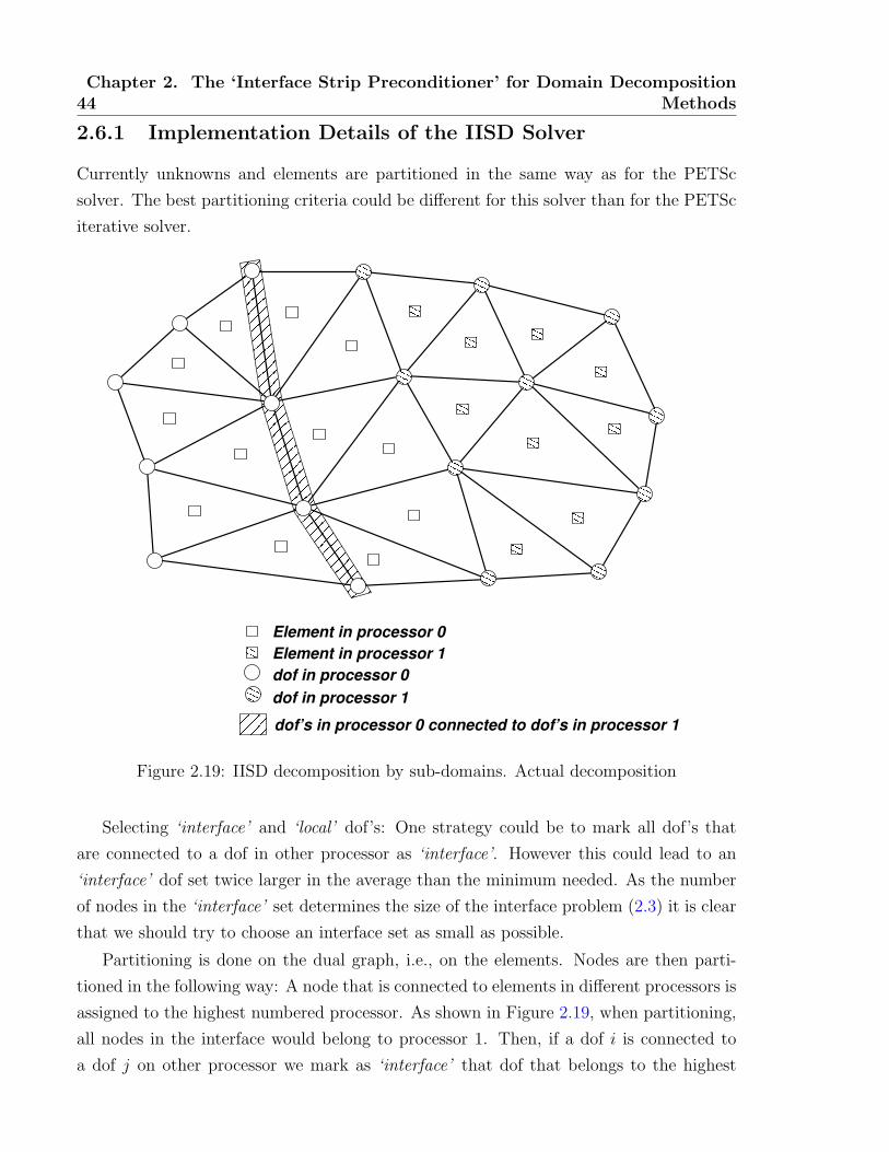
44Chapter 2. The ‘Interface Strip Preconditioner’ for Domain Decomposition
Methods
2.6.1 Implementation Details of the IISD Solver
Currently unknowns and elements are partitioned in the same way as for the PETSc
solver. The best partitioning criteria could be different for this solver than for the PETSc
iterative solver.
!!!!""""
####$$$$
%%%%&&&&
''((
))))****
++++,,
--..
Element in processor 1dof in processor 0dof in processor 1
dof’s in processor 0 connected to dof’s in processor 1
Element in processor 0
Figure 2.19: IISD decomposition by sub-domains. Actual decomposition
Selecting ‘interface’ and ‘local’ dof’s: One strategy could be to mark all dof’s that
are connected to a dof in other processor as ‘interface’. However this could lead to an
‘interface’ dof set twice larger in the average than the minimum needed. As the number
of nodes in the ‘interface’ set determines the size of the interface problem (2.3) it is clear
that we should try to choose an interface set as small as possible.
Partitioning is done on the dual graph, i.e., on the elements. Nodes are then parti-
tioned in the following way: A node that is connected to elements in different processors is
assigned to the highest numbered processor. As shown in Figure 2.19, when partitioning,
all nodes in the interface would belong to processor 1. Then, if a dof i is connected to
a dof j on other processor we mark as ‘interface’ that dof that belongs to the highest

2.6. The Interface Strip Preconditioner: Solution of the Strip Problem 45
numbered processor. In the mesh of Figure 2.19 all dof’s in the interface between element
sub-domains are marked to belong to processor 1. The nodes in the shadowed strip belong
to processor 0 and are connected to nodes in processor 1 but they are not marked as ‘in-
terface’ since they belong to the lowest numbered processor. Note that this strategy leads
to an interface set of 4 nodes, whereas the simpler strategy mentioned first would lead to
an interface set of 4 (i.e., including the nodes in the shadowed strip), which is two times
larger. The IISDMat matrix object contains three MPI PETSc matrices for the ALI , AIL
Proc 0 Proc 1
e
r
p
q
!!!!""""
##$$
%%%%&&&&
''''((
))**
Element in processor 0Element in processor 1dof in processor 0dof in processor 1
dof’s in processor 0 connected to dof’s in processor 1
Figure 2.20: Non local element contribution due to bad partitioning
and AII blocks and a sequential PETSc matrix on each processor for the local part of the
ALL block. The ALL block must be defined as sequential because otherwise we couldn’t
factorize it with the LU solver of PETSc. However this constrains that MatSetValues has
to be called in each processor for the matrix that belongs to its block, i.e., elements in
a given processor shouldn’t contribute to ALL elements in other processors. Normally,
this is so, but for some reasons this condition may be violated. One reason could be the
imposition of periodic boundary conditions and constraints in general (they are not taken
into account for the partitioning). Another reason is that a very bad partitioning may
46Chapter 2. The ‘Interface Strip Preconditioner’ for Domain Decomposition
Methods
arise in some not so common situations. Consider for instance Figure 2.20. Due to bad
partitioning a rather isolated element e belongs to processor 0, while being surrounded by
elements in processor 1. Now, as nodes are assigned to the highest numbered processor
of the elements connected to the node, nodes p, q and r are assigned to processor 1. But
then, nodes q and r will belong to the local subset of processor 1 but will receive contribu-
tions from element e in processor 0. However, the solution is not to define these matrices
as PETSc because, so far, PETSc does not support a distributed LU factorization. The
solution is to store those ALL contributions that belong to other processors in a temporary
buffer and after, to send those contributions to the correct processors directly with MPI
messages.
2.7 Classical Overlapping Domain Decomposition
Method: Alternating Schwarz Methods
The original alternating procedure described by Schwarz in 1870 consisted of three parts:
alternating between two overlapping domains, solving the Dirichlet problem on one do-
main at each iteration, and taking boundary conditions based on the most recent solution
obtained from the other domain. This procedure is called the Multiplicative Schwarz pro-
cedure. In matrix terms, this is very reminiscent of the block Gauß–Seidel iteration with
overlap defined with the help of projector operators. The analogue of the block-Jacobi
procedure is known as the Additive Schwarz procedure. A procedure that alternates be-
tween solving an equation in one sub-domain and then in the other one does not seem to
be parallel at the highest level because if one processor contains all of first sub-domain and
another processor contains all of second one then each processor must wait for the solution
of the other processor before it can execute Such approaches are known as multiplicative
approaches because of the form of the operator applied to the error. Alternatively, ap-
proaches that allow for the solution of sub-problems simultaneously are known as additive
methods. The difference is akin to the difference between Jacobi and Gauß–Seidel.
The analysis of the Schwarz methods as preconditioners was presented by Dryja and
Widlund in Reference [DW87] for the additive symmetric case and by Cai and Widlund
in [CW92] for the additive and multiplicative algorithms used in some nonsymmetric
problems. The successful application of Schwarz methods for solving symmetric elliptic
problems on stretched meshes was the inspiration to use them to solve the nonsymmetric
equations corresponding to discretization of flow problems. The algorithm can be sum-
marized as follows:

2.7. Classical Overlapping Domain DecompositionMethod: Alternating Schwarz Methods 47
Figure 2.21: Hermann Amandus Schwarz (1843–1921)
i) decompose the support mesh/grid into Ns overlapping sub-domains Ωi.
ii) each sub-domain Ωi is associated with the local space Vi. In addition, a coarse space
(often associated to a coarse mesh/grid) Vo ⊂ V (∪iVi) is defined. Subspaces Vi are used to
define the additive and multiplicative Schwarz methods, which can be identified with the
block-Jacobi method (if Ωi do not have common internal nodes) or with the Gauß–Seidel
method. The operators defining the two algorithms can be written as
M = I −Ns∑i=0
RTi A−1RiA and Mm = I −
Ns∏i=0
(I −RTi A−1RiA), (2.82)
where A is the global matrix and Ai, i = 1, ..., Ns, are the matrices associated with the
sub-domains Ωi. Projectors, Ri extract from the global vector of unknowns the dof’s
associated with Ωi, while projectors RTi extend by zeros dof’s of Ωi to the global vector.
Analogously, Ao is the matrix corresponding to Vo ⊂ V and Ro,RTo associate dof’s of
Vo with the global ones. Operators M and Mm consist of a sequence of local projection
operators Mi represented by matrices RTi A−1RiA.
iii) according to the idea of preconditioning by the standard iteration Krylov-like methods
are used to solve the preconditioned systems P−1(Au − f) = 0 with the preconditioner
P−1 = (I −M)A−1 or P−1 = (I −Mm)A−1.

48Chapter 2. The ‘Interface Strip Preconditioner’ for Domain Decomposition
Methods
2.8 Conclusions
A new preconditioner for Schur complement domain decomposition methods was theo-
retically presented. This preconditioner is based on solving a global problem posed in a
narrow strip around the inter-subdomain interfaces. Some analytical results have been
derived to present its mathematical basis. Numerical experiments will be carried out in
next chapters to show its convergence properties and performance.
The IS preconditioner is easy to construct because it does not require any special
calculation (it can be assembled with a subset of sub-domain matrices coefficients). It is
much less memory-consuming than classical optimal preconditioners such as Neumann-
Neumann in primal methods (or Dirichlet in FETI methods). Moreover, it permits to
decide how much memory to assign for preconditioning purposes.
In advective-diffusive real-life problems, where the Peclet number can vary on the
domain between low and high values, the proposed preconditioner outperforms classical
ones in advection-dominated regions while it is capable to handle reasonably well diffusion-
dominated regions.
Chapter 3
Numerical Tests
There is a concept
which corrupts and upsets all others.
I refer not to Evil, whose limited realm is that of ethics;
I refer to the infinite.
‘The Avatars of the Tortoise’, Jorge Luis Borges
This chapter is dedicated to confirm theoretical results developed in previous chapters
with numerical examples. The examples cover a vast number of physical problems and
applications in computational fluid dynamics and mechanics areas that range from simple
scalar diffusive advective models to viscous/inviscid compressible/incompressible Navier-
Stokes at high Mach and Reynolds numbers models, coupled surface/subsurface water
flow over complex large scale domains, etc. Also, the performance of the preconditioner
is studied in the context of monolithic and disaggregated time integration schemes. The
use of this new solver is extended to two major problems in CFD like general dynamics
boundary conditions imposition and weak/strong fluid/structure interaction in chapters §4and §5.
The problems presented in this thesis were solved using the PETSc-FEM code (see
Reference [SNPD06]), a general purpose, parallel, multi-physics FEM program for CFD
applications based on MPI and PETSc libraries (see [GLS94] and [BGCMS04], respec-
tively). PETSc-FEM comprises both a library that allows the user to develop FEM
49
50 Chapter 3. Numerical Tests
(or FEM-like, i.e., unstructured mesh oriented) programs, and a suite of application
programs (e.g., compressible/incompressible Navier-Stokes, multi-phase flow, compress-
ible Euler equations, shallow water model, general advective-diffusive systems, coupled
surface/subsurface water flow over multi-aquifer systems, linear elasticity and Laplace
equation, weak/strong fluid-structure interaction, multiphase flow). Mesh partitioning is
performed by using METIS and the library takes in charge of passing the appropriate
elements to each processor, to find out the vectors, to assemble the residual and matrices,
and to fix the boundary conditions, for all the processors.
Figure 3.1: Leonhard Euler (1707–1783)
3.1 Numerical Examples in Sequential Environments
3.1.1 The Poisson’s Problem
The performance of the proposed preconditioner is compared in a sequential environment.
For this purpose, we consider two different problems. The domain Ω in both cases is the
unit square discretized on an unstructured mesh of 120×120 nodes, and decomposed in 6
rectangular sub-domains. We compare the residual norm versus iteration count by using
no preconditioner, Neumann-Neumann preconditioner, and the IS preconditioner (with
several node layers at each interface side).
The first example is the Poisson’s problem ∆φ = g, where g = 1 and φ = 0 on all the
boundary Γ. The iteration counts and the problem solution (obtained in a coarse mesh
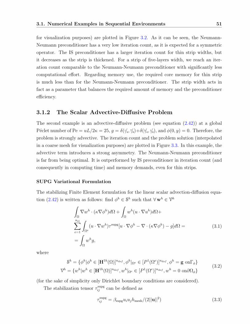
3.1. Numerical Examples in Sequential Environments 51
for visualization purposes) are plotted in Figure 3.2. As it can be seen, the Neumann-
Neumann preconditioner has a very low iteration count, as it is expected for a symmetric
operator. The IS preconditioner has a larger iteration count for thin strip widths, but
it decreases as the strip is thickened. For a strip of five-layers width, we reach an iter-
ation count comparable to the Neumann-Neumann preconditioner with significantly less
computational effort. Regarding memory use, the required core memory for thin strip
is much less than for the Neumann-Neumann preconditioner. The strip width acts in
fact as a parameter that balances the required amount of memory and the preconditioner
efficiency.
3.1.2 The Scalar Advective-Diffusive Problem
The second example is an advective-diffusive problem (see equation (2.42)) at a global
Peclet number of Pe = uL/2κ = 25, g = δ(1/4, 7/8)+δ(3/4, 1/8), and φ(0, y) = 0. Therefore, the
problem is strongly advective. The iteration count and the problem solution (interpolated
in a coarse mesh for visualization purposes) are plotted in Figure 3.3. In this example, the
advective term introduces a strong asymmetry. The Neumann-Neumann preconditioner
is far from being optimal. It is outperformed by IS preconditioner in iteration count (and
consequently in computing time) and memory demands, even for thin strips.
SUPG Variational Formulation
The stabilizing Finite Element formulation for the linear scalar advection-diffusion equa-
tion (2.42) is written as follows: find φh ∈ Sh such that ∀wh ∈ Vh∫Ω
∇wh · (κ∇φh)dΩ +
∫Ω
wh(u · ∇uh)dΩ+
nel∑e=1
∫Ωe
(u · ∇wh)τ supg[u · ∇φh −∇ · (κ∇φh)− g]dΩ =
=
∫Ω
whg,
(3.1)
where
Sh = φh|φh ∈ [H1h(Ω)]ndof , φh|Ωe ∈ [P 1(Ωe)]ndof , φh = g onΓφ
Vh = wh|wh ∈ [H1h(Ω)]ndof , wh|Ωe ∈ [P 1(Ωe)]ndof , wh = 0 on∂Ωφ(3.2)
(for the sake of simplicity only Dirichlet boundary conditions are considered).
The stabilization tensor τ supgij can be defined as
τ supgij = βsupguiujhmesh/(2||u||2) (3.3)

52 Chapter 3. Numerical Tests
0 20 30 40 50 60
10−7
10−6
10−5
10−4
10−3
10−2
10−1
100
101
iteration number10
ISP n=1 layers
not preconditioned
n=2n=3
n=4
n=5Neumann−Neumann
Figure 3.2: Solution of Poisson’s problem
0 5 10 15 20 25 30 35
10−7
10−6
10−5
10−4
10−3
10−2
10−1
100
101
iteration number
not preconditionedISP n=1 layers
Neumann−Neumann
n=2n=3
n=4n=5
Figure 3.3: Solution of advective-diffusive problem
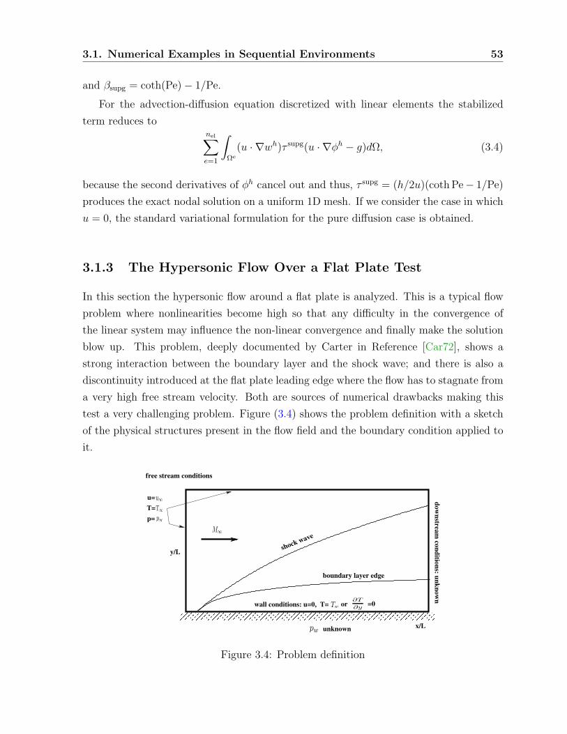
3.1. Numerical Examples in Sequential Environments 53
and βsupg = coth(Pe)− 1/Pe.
For the advection-diffusion equation discretized with linear elements the stabilized
term reduces tonel∑e=1
∫Ωe
(u · ∇wh)τ supg(u · ∇φh − g)dΩ, (3.4)
because the second derivatives of φh cancel out and thus, τ supg = (h/2u)(coth Pe− 1/Pe)
produces the exact nodal solution on a uniform 1D mesh. If we consider the case in which
u = 0, the standard variational formulation for the pure diffusion case is obtained.
3.1.3 The Hypersonic Flow Over a Flat Plate Test
In this section the hypersonic flow around a flat plate is analyzed. This is a typical flow
problem where nonlinearities become high so that any difficulty in the convergence of
the linear system may influence the non-linear convergence and finally make the solution
blow up. This problem, deeply documented by Carter in Reference [Car72], shows a
strong interaction between the boundary layer and the shock wave; and there is also a
discontinuity introduced at the flat plate leading edge where the flow has to stagnate from
a very high free stream velocity. Both are sources of numerical drawbacks making this
test a very challenging problem. Figure (3.4) shows the problem definition with a sketch
of the physical structures present in the flow field and the boundary condition applied to
it.
M∞
Tw
∂T
∂y
pw
p∞
T∞
u∞
boundary layer edge
x/L
y/L shock wave
free stream conditions
downstream
conditions: unknown
unknown
T=p=
u=
or =0wall conditions: u=0, T=
Figure 3.4: Problem definition

54 Chapter 3. Numerical Tests
Physical Model
We focus this test in the solution of compressible Navier-Stokes equations with the
SUPG/SC (“Streamline Upwind Petrov-Galerkin/Shock Capturing”) method proposed
by Brooks et al. in Reference [BH82] and by Aliabady et al. in Reference [ART93]. The
differential form of the conservation equations of mass, momentum and total energy that
governs the dynamics of compressible and viscous fluid flow may be written in a compact
intrinsic (vector) form as (Einstein summation convention is assumed, i, j = 1, 2, 3)
Figure 3.5: Claude Louis Marie Henri Navier (1785–1836)
Figure 3.6: George Gabriel Stokes (1819–1903)
∂U
∂t+∂(Fa)i
∂xi
=∂(Fd)i
∂xi
+ G in Ω× (0, t+], (3.5)
where Ω is the model domain with boundary Γ. U = (ρ, ρu, ρe)t is the unknown state
vector expressed in conservative variables as above, e represents the specific total energy,

3.1. Numerical Examples in Sequential Environments 55
Fa accounts for the (vector) advective fluxes, Fd for the (vector) diffusive fluxes and G is
used for the external source terms (i.e, G = (0, ρfe,Wf + qH), Wf = ρfe · u is the work
done by the external forces fe and n represents the boundary unit normal vector). Also,
initial and boundary condition must be added (see [Hir90]). In this thesis, we treat the
so-called absorbent boundary conditions (see chapter §4). The integral conservation form
is
∂
∂t
∫Ω
ρ
ρu
ρE
dΩ +
∮Γ
ρu
ρu⊗ u + pI − τ
ρuH − τ · u− k∇T
· ndΓ =
∫Ω
0
ρfe
Wf + qH
dΩ. (3.6)
In (3.6), H is the total specific enthalpy defined in terms of the specific internal energy
h and the specific kinetic energy as H = e + p/ρ + 1/2|u|2 = E + p/ρ and h = e + p/ρ,
respectively. The above mentioned advective and diffusive fluxes are defined as
Fa =
ρui
ρu1ui + δi1p
ρu2ui + δi2p
ρu3ui + δi3p
(ρE + p)ui
, Fd =
0
τi1
τi2
τi3
τikuk − qi
. (3.7)
Here δij is the Kronecker isotropic tensor of rank 2 (also denoted as I), and τij are the
components of the Newtonian viscous stress tensor τij = 2µεij(u) − 2/3µ(∇ · u)δij. The
strain rate tensor εij is εij(u) = 12(∂jui + ∂iuj) and qi is the heat flux defined according
to the Fourier law assumptions as qi = −κ∇T with κ the thermal conductivity and
T the absolute temperature. The coefficients of viscosity and thermal conductivity are
assumed to be given by the Sutherland formula (i.e, the gas is considered in a standard
atmosphere),
µ = µ0
(T
T0
)3/2T0 + 110
T + 110κ =
γRµ
(γ − 1)Pr, (3.8)
where µ0 is the viscosity at the reference temperature T0 and Pr is the Prandtl number
(i.e., Pr = ν/ι, ι is the thermal diffusivity coefficient).
The physical model is closed by the definition of the constitutive law for the specific
internal energy in terms of the thermodynamic state and some state equation for the
thermodynamic variables. Normally an ideal gas law is adopted, then ρe = pγ−1
+ 1/2ρ||u||2
and p = ρRT , where R = (γ− 1)Cv is the particular gas constant and γ = Cp
Cvis the ratio
of the specific heat at constant pressure relative to that at constant volume. Alternatively,

56 Chapter 3. Numerical Tests
Figure 3.7: Leopold Kronecker (1823–1891)
equation (3.6) can be written in the quasi-linear form
∂U
∂t+ Ai
∂U
∂xi
=∂
∂xi
(Kij
∂U
∂xj
)+ G (3.9)
where the assumption that the flux vectors are only function of the state variables, i.e.,
Fa = Fa(U) and Fd = Fd(U) is made. Then, the divergence of the flux vector functions
can be written as
∂Fa
∂xi
=∂Fa
∂U
∂U
∂xi
= Ai∂U
∂xi
(3.10)
and
∂Fd
∂xi
=∂Fd
∂U
∂U
∂xi
= Kij∂U
∂xi
. (3.11)
Inviscid Approximation
In some particular cases, when inertial forces are predominant over viscous effects and
no heat conduction is considered, the fluid motion is described by the Euler equations
and they are obtained from the Navier-Stokes equations neglecting all shear stresses and
heat conduction terms. This is a valid approximation for flows at high Reynolds numbers
(Re = ||u||L/ν, L is a characteristic length scale and ν is the kinematic viscosity). The
use of this approach changes the mathematical behavior of the set of equations. The set of
differential equations becomes first order and hyperbolic. The boundary conditions must
be reformulated and the solution can accept discontinuous variables. The imposition of
non-reflecting boundary conditions will be treated further.

3.1. Numerical Examples in Sequential Environments 57
Figure 3.8: Osborne Reynolds (1842–1912)
Variational Formulation
In this section, the variational formulation of the compressible Navier-Stokes equations
using SUPG Finite Element Method and the shock capturing operator is presented. Con-
sider a finite element discretization of the Ω into sub-domains Ωe, e = 1, 2, . . . , nel. Based
on this discretization, the finite element function spaces for the trial solutions and for
the weighting functions, Vh and Sh respectively, can be defined. These function spaces
are selected as subsets of [H1h(Ω)]ndof when taking Dirichlet boundary conditions, where
H1h(Ω) is the finite dimensional Sobolev functional space over Ω, and ndof = nsd + 2 is
the number of dof’s in the continuum problem (nsd is the number of spatial dimensions).
The stabilizing finite element formulation of the quasi-linear form of (3.5) is written
as follows: find Uh ∈ Sh such that ∀Wh ∈ Vh∫Ω
Wh ·(∂Uh
∂t+∂Fh
a
∂xi
)dΩ =
∫Ω
Wh ·(∂Fh
d
∂xi
+ G
)dΩ∫
Ω
Wh ·(∂Uh
∂t+ Ah
i
∂Uh
∂xi
− G
)dΩ +
∫Ω
∂Wh
∂xi
·Khij
∂Uh
∂xj
dΩ−∫
Γh
Wh ·HhdΓ+
+
nel∑e=1
∫Ωe
τ(Ahk)
T ∂Wh
∂xk
·∂Uh
∂t+ Ah
i
∂Uh
∂xi
− ∂
∂xi
(Kh
ij
∂Uh
∂xj
)− G
dΩ+
+
nel∑e=1
∫Ωe
δshc∂Wh
∂xi
· ∂Uh
∂xi
dΩ = 0,
(3.12)
where
Sh = Uh|Uh ∈ [H1h(Ω)]ndof ,Uh|Ωe ∈ [P 1(Ωe)]ndof ,Uh = g onΓg
Vh = Wh|Wh ∈ [H1h(Ω)]ndof ,Wh|Ωe ∈ [P 1(Ωe)]ndof ,Wh = 0 on∂Ωg,(3.13)
58 Chapter 3. Numerical Tests
and where matrices Ai and Kij are defined in section §3.1.3.
The first three terms inside the first two integrals in the variational formulation (3.12)
constitute the Galerkin formulation of the problem and the third integral accounts for the
Neumann boundary conditions. The first series of element level integrals in (3.12) are the
SUPG stabilization terms added to prevent spatial oscillations in the advection-dominated
range. The second series of element level integrals in (3.12) are the shock capturing terms
added to assure the stability at high Mach and Reynolds number flows, specially to sup-
press spurious overshoot and undershoot effects in the vicinity of discontinuities. Various
Figure 3.9: Ernst Mach (1838–1916)
options for calculating the stabilization parameters and defining the shock capturing terms
in the context of the SUPG formulation were introduced in Reference [TMRS92]. In this
section we describe some of these options. The first one is the standard SUPG intrinsic
time tensor τ introduced by Aliabadi and Tezduyar in Reference [ART93]. In this case
this matrix is defined as τ = max[0, τa − τd − τδ], with each τx taking into account the
advective and diffusive effects and also avoiding the duplication of the shock capturing
operator and the streamline upwind operator. These matrices are defined as
τa =h
2(c+ |u|)I, τd =
∑nsd
j=1 β2j diag (Kjj)
(c+ |u|)2I, τδ =
δshc
(c+ |u|)2I, (3.14)
where c is the acoustic speed, h = 2(∑nen
a=1 |u · ∇Na|)−1
is the element size computed
here as the element length in the direction of the streamline using for its definition the
multi-lineal trial function Na and δshc is the shock capturing parameter defined in the
next paragraph. The τ matrix computation is already an open problem because it is
not possible to diagonalize the system of equations. It follows some heuristics arguments
based on the maximum value of the set of eigenvalues of the advective Jacobian matrices
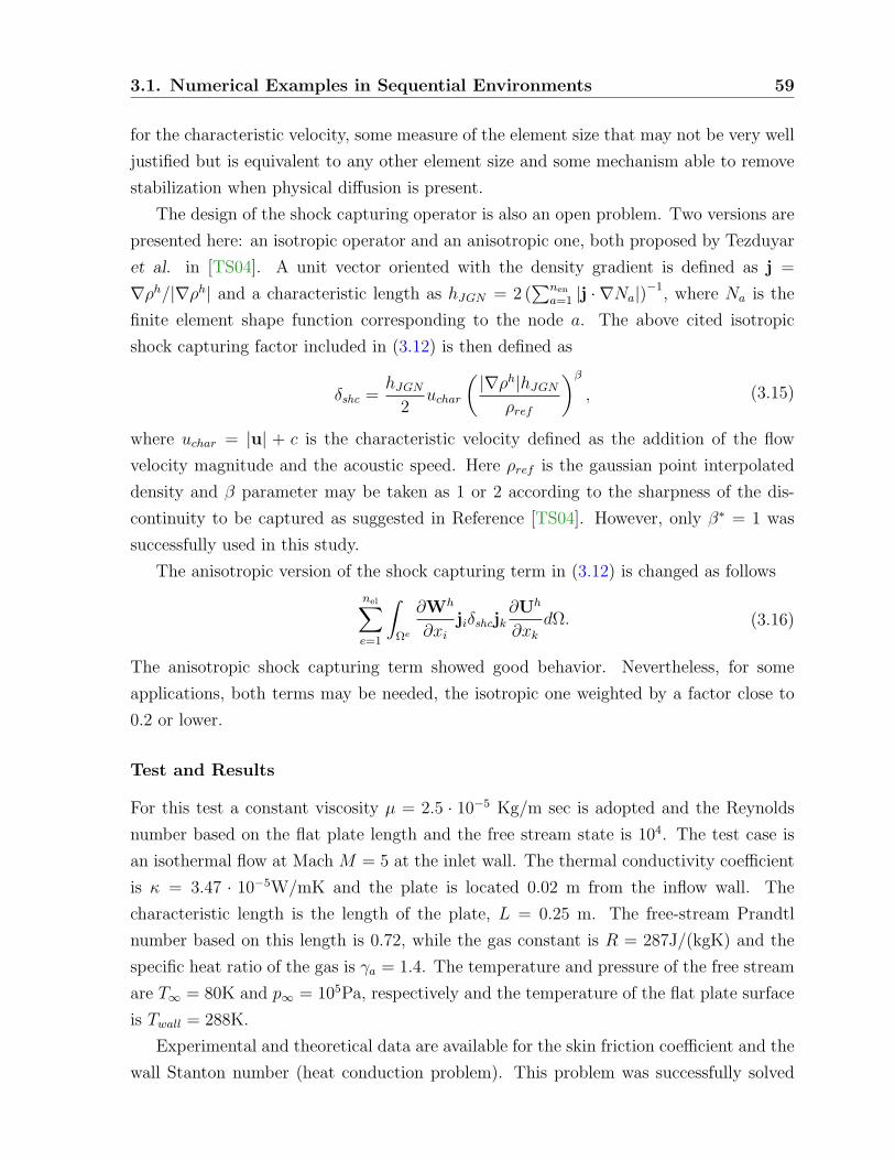
3.1. Numerical Examples in Sequential Environments 59
for the characteristic velocity, some measure of the element size that may not be very well
justified but is equivalent to any other element size and some mechanism able to remove
stabilization when physical diffusion is present.
The design of the shock capturing operator is also an open problem. Two versions are
presented here: an isotropic operator and an anisotropic one, both proposed by Tezduyar
et al. in [TS04]. A unit vector oriented with the density gradient is defined as j =
∇ρh/|∇ρh| and a characteristic length as hJGN = 2 (∑nen
a=1 |j · ∇Na|)−1, where Na is the
finite element shape function corresponding to the node a. The above cited isotropic
shock capturing factor included in (3.12) is then defined as
δshc =hJGN
2uchar
(|∇ρh|hJGN
ρref
)β
, (3.15)
where uchar = |u| + c is the characteristic velocity defined as the addition of the flow
velocity magnitude and the acoustic speed. Here ρref is the gaussian point interpolated
density and β parameter may be taken as 1 or 2 according to the sharpness of the dis-
continuity to be captured as suggested in Reference [TS04]. However, only β∗ = 1 was
successfully used in this study.
The anisotropic version of the shock capturing term in (3.12) is changed as follows
nel∑e=1
∫Ωe
∂Wh
∂xi
jiδshcjk∂Uh
∂xk
dΩ. (3.16)
The anisotropic shock capturing term showed good behavior. Nevertheless, for some
applications, both terms may be needed, the isotropic one weighted by a factor close to
0.2 or lower.
Test and Results
For this test a constant viscosity µ = 2.5 · 10−5 Kg/m sec is adopted and the Reynolds
number based on the flat plate length and the free stream state is 104. The test case is
an isothermal flow at Mach M = 5 at the inlet wall. The thermal conductivity coefficient
is κ = 3.47 · 10−5W/mK and the plate is located 0.02 m from the inflow wall. The
characteristic length is the length of the plate, L = 0.25 m. The free-stream Prandtl
number based on this length is 0.72, while the gas constant is R = 287J/(kgK) and the
specific heat ratio of the gas is γa = 1.4. The temperature and pressure of the free stream
are T∞ = 80K and p∞ = 105Pa, respectively and the temperature of the flat plate surface
is Twall = 288K.
Experimental and theoretical data are available for the skin friction coefficient and the
wall Stanton number (heat conduction problem). This problem was successfully solved

60 Chapter 3. Numerical Tests
using the IISD+ISP solver and the overlapping additive Schwarz preconditioner, but
it was not possible to obtain a solution with a Global GMRes with diagonal scaling
preconditioner (i.e., GMRes over the whole matrix with point Jacobi preconditioning)
solver, using for the three cases a Krylov subspace dimension of 200. In the latter case,
the solution presented poor resolution of the strong shock wave after some time steps
and finally crashed. It should be remarked that up to M = 2.5 preconditioned Global
GMRes iteration works fine, giving results in agreement with experimental results and
theoretical approaches. The number of sub-domains used for the IISD+ISP case is 4.
For the Schwarz scheme, 4 sub-blocks (an ILU(0) solver is used on each block) and an
overlapping of a single layer of nodes around the interface between the blocks are used.
This kind of example is for cases where the computational resources are limited to
a single processor architecture and it is not possible to get a solution using the precon-
ditioned Global GMRes scheme. The mesh used was composed by 24150 quadrangular
elements and 24462 nodes. In order to capture the high thermal and flow gradients, the
normal spacing close to the flat plate was chosen about 4 ·10−6 and the time step adopted
was ∆t = 0.005. The initial state adopted is a stationary flow at Mach 2.5 at the inlet,
previously obtained via the IISD+ISP method. Two Newton loops were used for the
non-linear problem.
Figures (3.10) and (3.11) show the skin friction coefficient and the Stanton number
against theoretical predictions based on analytical solutions of an approximate theory
called Eckert reference enthalpy method [GLD94]. These results show a good behavior of
the numerical results relative to the analytical predictions. The test was conducted in a
PC Pentium IV - 2.8 GHz (RAM DDR, 400 MHz). The CPU time per time steps (i.e.,
less than 3 minutes in average) and the residual convergence rate (roughly 150-170 itera-
tions to converge 7 orders of magnitude) were comparable for both domain decomposition
methods. In the IISD+ISP solver, the sub-domain problems are solved with a LU de-
composition with nested dissection reordering. If complete LU factorization is used in the
Schwarz method, the memory requirements and CPU time per time steps are increased.
3.2 Numerical Examples in Parallel Environment
In this section, we present numerical results for diffusive and advective problems and some
discussions about these results. The tests were carried out on a Beowulf cluster of PC’s.
The cluster at CIMEC laboratory has twenty (uniprocessor) nodes, where 10 nodes are
Pentium IV - 2.4 GHz, 1 GB RAM (DDR, 333 MHz), 7 nodes Pentium IV - 1.7 GHz,
512 MB RAM (RIMM, 400/800 MHz) and 2 nodes Pentium IV 1.7 GHz, 256 MB RAM

3.2. Numerical Examples in Parallel Environment 61
0 0.05 0.1 0.15 0.2 0.25−0.05
0
0.05
0.1
0.15
0.2
0.25
0.3
0.35
0.4
0.45
skin
fric
tion
coef
ficie
nt
coordinate along plate
IISD+ISPAdditive Schwarztheoretical
Figure 3.10: Skin friction coefficient
0 0.05 0.1 0.15 0.2 0.2510−3
10−2
10−1
100
Sta
nton
num
ber
coordinate along plate
IISD+ISPAdditive Schwarztheoretical
Figure 3.11: Stanton number

62 Chapter 3. Numerical Tests
Table 3.1: CPU time and memory requirements per proc. for Poisson problem (mesh 500×500 elements). Note: * in table means iteration failed to converge to a specified tolerance
in a maximum of 200 its.
Precond. none Jacobi glob. block − Jacobi N −N ISP (nlay = 1) ISP (nlay = 5)
factoriz. [secs] - - 1.9 4.7 2.3 2.3
CG st. [secs] * * * 1.51 5.4 4.9
tolerance 1.e-10 1.e-10 1.e-10 1.e-10 1.e-10 1.e-10
mem./proc [Mb] * * * 70 62 62.5
(RIMM, 400/800 MHz). Usually, the first node works as server. The nodes are connected
through a switch Fast Ethernet (100 Mbit/sec, latency=O(100) µsecs).
The performance of the proposed preconditioner is studied in a parallel environment.
For this purpose, we consider two different problems. The domain Ω in both cases is
the unit square discretized on an structured mesh of 500 × 500 nodes, and decomposed
in 4 rectangular sub-domains. We compare the residual norm versus iteration count by
using no preconditioner, Neumann-Neumann preconditioner, block-Jacobi preconditioner,
Global Jacobi preconditioner and the IS preconditioner (with several strip widths at the
interfaces). Global Jacobi is a diagonal scaling preconditioning algorithm. Block-Jacobi
preconditioner is a block-diagonal preconditioner and is obtained by (approximately) in-
verting the local diagonal blocks on each processor (see [Saa00] for a detailed description
of these preconditioners).
3.2.1 The Poisson’s Problem
As in the sequential run (section §3.1.1), the parallel version of this test has shown a good
behavior in terms of performance related to the classical preconditioners and the global
solution. The iteration counts and the problem solution are plotted in Figure 3.12. We
split the system solution in two stages, the factorization stage (for the local problems) and
the GMRes iteration stage (including the Richardson iteration for the IS preconditioner),
in order to compute the time consumed to achieve a given tolerance in the residual vector
(see Table 3.1). CPU times for the iteration stage and memory requirements are not
given in Table 3.1 for Jacobi preconditioning and not preconditioning at all because these
methods failed to converge.

3.2. Numerical Examples in Parallel Environment 63
1e−12
1e−10
1e−08
1e−06
0.0001
0.01
1
0 10 20 30 40 50 60 70 80
90 100
resi
dual
nor
m =
||r(
n)||/
||r(0
)||
iteration number
Neumann−Neumann
IS n=1 layers
IS n=5 layers
Block jacobi NoneJacobiglobal
Figure 3.12: Solution of Poisson’s problem (mesh 500× 500 elements)
3.2.2 The Scalar Advective-Diffusive Problem
The second example is an advective-diffusive problem at a global Peclet number of
Pe = 25, g = δ(1/4, 3/4) + δ(3/4, 1/4), and φ(−0.5, y) = 0, where δ is the Dirac’s delta func-
tion. Therefore, the problem is strongly advective. We compare the iteration counts in
two different meshes and two different decompositions. The mesh of 500 × 500 nodes is
decomposed in 4 rectangular domains, one per processor, and the mesh of 1000 × 1000
is partitioned into 7 sub-domains. The iteration count and the problem solution (inter-
polated in a coarse mesh for visualization purposes) are plotted in Figures 3.13 and 3.14.
In this example, the advective term introduces a strong asymmetry. CPU times and
memory requirements are not given in Table 3.2 for N-N preconditioner because this
method failed to converge. However, only to give an idea, the required memory for N-
N preconditioner (coarse mesh) for 50/60 iterations (IS was converged at this point) is
73 Mb/proc (megabytes per processor), whereas for 200 iterations (the maximum al-
lowed) the consumed memory was 120 Mb/proc. For the refined mesh, the memory used
in 70/80 iterations is 210 Mb/proc and for the 200 iterations (the maximum allowed)
was 320 Mb/proc. Clearly, the Neumann-Neumann preconditioner is outperformed by
IS preconditioner in iteration count (and consequently in computing time) and memory
demands, even for thin strips. The CPU time and memory used (per processor) are shown
in Table 3.2.
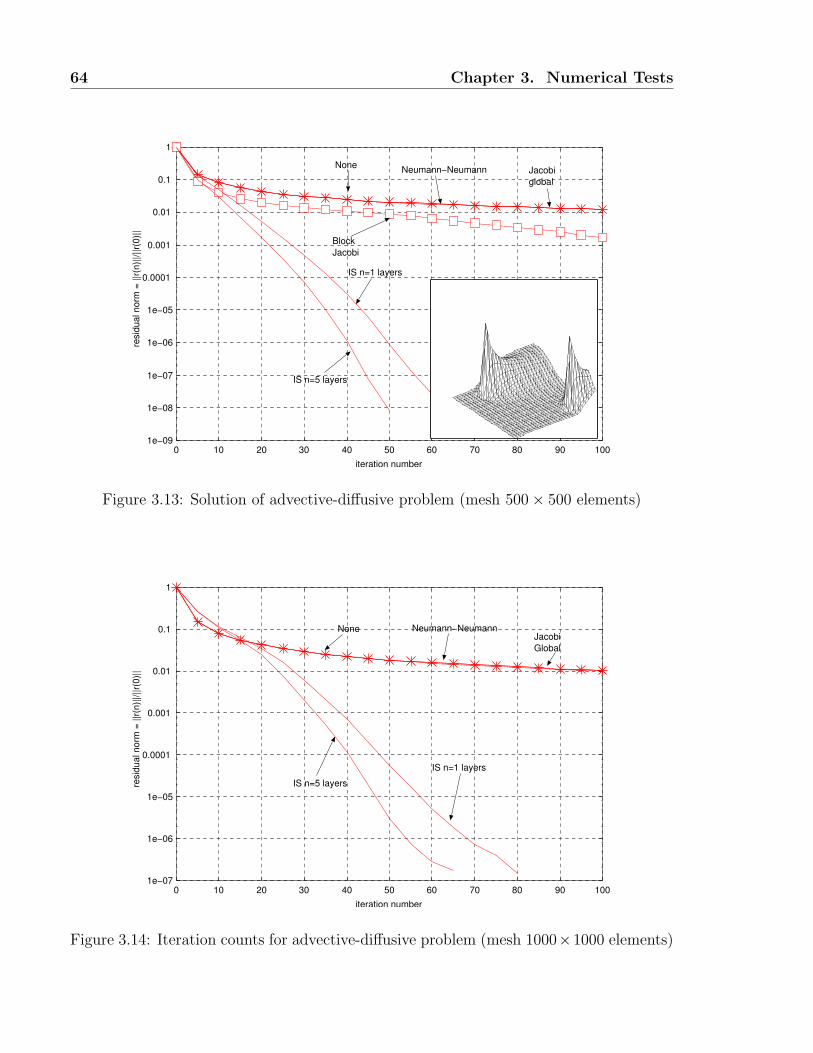
64 Chapter 3. Numerical Tests
1e−09
1e−08
1e−07
1e−06
1e−05
0.0001
0.001
0.01
0.1
1
0 10 20 30 40 50 60 70 80 90 100
resi
dual
nor
m =
||r(
n)||/
||r(0
)||
iteration number
IS n=1 layers
IS n=5 layers
BlockJacobi
None Jacobiglobal
Neumann−Neumann
Figure 3.13: Solution of advective-diffusive problem (mesh 500× 500 elements)
1e−07
1e−06
1e−05
0.0001
0.001
0.01
0.1
1
0 10 20 30 40 50 60 70 80 90 100
resi
dual
nor
m =
||r(
n)||/
||r(0
)||
iteration number
IS n=5 layers
IS n=1 layers
NoneJacobiGlobal
Neumann−Neumann
Figure 3.14: Iteration counts for advective-diffusive problem (mesh 1000×1000 elements)

3.2. Numerical Examples in Parallel Environment 65
Table 3.2: CPU time and memory requirements per proc. for advective-diffusive problem
(mesh 1000 × 1000 elements). Note: * in table means iteration failed to converge to a
specified tolerance in a maximum of 200 its.
Preconditioner none Jacobi glob. N −N ISP (nlay = 1) ISP (nlay = 5)
factoriz. [secs] - - 4.0 8.0 7.8
GMRes st. [secs] * * * 13.0 12.0
tolerance 0.25e-06 0.25e-06 0.25e-06 0.25e-06 0.25e-06
mem./proc. [Mb] * * * 140 142
3.2.3 The Coupled Hydrological Flow Model
Subsurface Flow
The equation for the flow in a confined (phreatic) aquifer integrated in the vertical direc-
tion is∂
∂t(S(φ− η)φ) = ∇ · (K(φ− η)∇φ) +
∑Ga, on Ωaq × (0, t], (3.17)
where the per-node property η represents the height of the aquifer bottom to a given
datum. The corresponding unknown for each node is the piezometric height or the level
of the phreatic surface at that point φ and Ωaq is the aquifer domain, S the storativity,
K the hydraulic conductivity and Ga is a source term, due to rain, losses from streams
or other aquifers.
Surface flow [Whi74, Hir90]
2D Saint-Venant Model. The equations for the 2D Saint-Venant open channel flow
are the well known mass and momentum conservation equations integrated in the ver-
tical direction. If we write these equations in the conservation matrix form (Einstein
summation convention is assumed), we have
∂U
∂t+∂Fi(U)
∂xi
= Gi(U), i = 1, 2, on Ωst × (0, t], (3.18)
where Ωst is the stream domain, U = (h, hu, hv)T is the state vector and the advective
flux functions in (3.18) are
F1(U) = (hu, hu2 + gh2
2, huv)T ,
F2(U) = (hv, huv, hv2 + gh2
2)T ,
(3.19)

66 Chapter 3. Numerical Tests
Figure 3.15: Adhemar Jean Claude Barre de Saint-Venant (1797–1886)
where h is the height of the water in the channel with respect to the channel bottom,
u = (u, v)T is the velocity vector and g is the acceleration due to gravity. Here Gs
represents the gain (or loss) of the river, the source term is
G(U) = (Gs, gh(S0x − Sfx), gh(S0y − Sfy))T , (3.20)
where S0 is the bottom slope and Sf is the slope friction, given by
Sfx =1
C2hhu|u|, Sfy =
1
C2hhv|u| for the Chezy model,
Sfx =n2
h4/3u|u|, Sfy =
n2
h4/3v|u| for the Manning model,
(3.21)
where Ch and n (the Manning roughness) are model constants. In the case of great
lakes, wide rivers and estuaries we should take in account the effect of Coriolis force
(see [PSI+03]).
1D Saint-Venant Model. When velocity variations on the channel cross section are
neglected, the flow can be treated as one dimensional. The equations of mass and mo-
mentum conservation on a variable cross sectional stream (in conservation form) are
∂A(s, t)
∂t+∂Q(A(s, t))
∂s= Gs(s, t),
1
A(s, t)
∂Q
∂t+
1
A(s, t)
∂
∂s(β
Q2
A(s, t)) + g(S0 − Sf )+
+g∂h
∂s=
qtA(s, t)
(v − vt), on Ωst × (0, t],
(3.22)
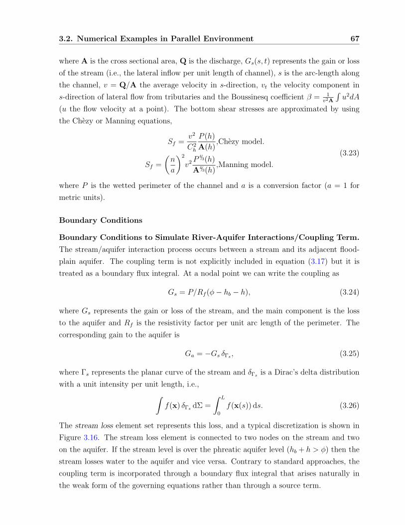
3.2. Numerical Examples in Parallel Environment 67
where A is the cross sectional area, Q is the discharge, Gs(s, t) represents the gain or loss
of the stream (i.e., the lateral inflow per unit length of channel), s is the arc-length along
the channel, v = Q/A the average velocity in s-direction, vt the velocity component in
s-direction of lateral flow from tributaries and the Boussinesq coefficient β = 1v2A
∫u2dA
(u the flow velocity at a point). The bottom shear stresses are approximated by using
the Chezy or Manning equations,
Sf =v2
C2h
P (h)
A(h),Chezy model.
Sf =
(n
a
)2
v2P4/3(h)
A4/3(h),Manning model.
(3.23)
where P is the wetted perimeter of the channel and a is a conversion factor (a = 1 for
metric units).
Boundary Conditions
Boundary Conditions to Simulate River-Aquifer Interactions/Coupling Term.
The stream/aquifer interaction process occurs between a stream and its adjacent flood-
plain aquifer. The coupling term is not explicitly included in equation (3.17) but it is
treated as a boundary flux integral. At a nodal point we can write the coupling as
Gs = P/Rf (φ− hb − h), (3.24)
where Gs represents the gain or loss of the stream, and the main component is the loss
to the aquifer and Rf is the resistivity factor per unit arc length of the perimeter. The
corresponding gain to the aquifer is
Ga = −Gs δΓs , (3.25)
where Γs represents the planar curve of the stream and δΓs is a Dirac’s delta distribution
with a unit intensity per unit length, i.e.,∫f(x) δΓs dΣ =
∫ L
0
f(x(s)) ds. (3.26)
The stream loss element set represents this loss, and a typical discretization is shown in
Figure 3.16. The stream loss element is connected to two nodes on the stream and two
on the aquifer. If the stream level is over the phreatic aquifer level (hb + h > φ) then the
stream losses water to the aquifer and vice versa. Contrary to standard approaches, the
coupling term is incorporated through a boundary flux integral that arises naturally in
the weak form of the governing equations rather than through a source term.

68 Chapter 3. Numerical Tests
x
y
stream
aquifer node
stream node
n1n2
n3
n4
n5
Figure 3.16: Stream/Aquifer coupling
Initial Conditions. First, Second and Third Kind Boundary Conditions. Ground-
water flow. In the previous section, the equation that governs subsurface flow was es-
tablished. In order to obtain a well posed PDE problem, initial and boundary conditions
must be superimposed on the flow domain and on its limits. The initial condition for the
groundwater problem is a constant hydraulic head in the whole region that obeys levels
observed in the basin history.
Now, consider a simply connected region Ω bounded by a closed curve ∂Ω such that
∂Ωφ ∪ ∂Ωσ ∪ ∂Ωφσ = ∂Ω. We consider the stream partially penetrating and connected, in
a Hydraulic sense, to the aquifer, hence, we set
φ = φ0, on ∂Ωφ × (0, t]
K(φ− η)∂φ
∂n= σ0, on ∂Ωσ × (0, t]
K(φ− η)∂φ
∂n= C(φ− h), on ∂Ωφσ × (0, t],
(3.27)
where φ0 is a given water head, σ0 is a given flux normal to the flux boundary ∂Ωσ and
C the conductance at the river/stream interface.
Surface Flow - Fluid Boundary. We recall that the type of a flow in a stream or in
an open channel depends on the value of the Froude number Fr = |u|/c (where c =√gh
is the wave celerity). A flow is said
• fluvial, for |u| < c.
• torrential, for |u| > c.
Saint-Venant Equations. Fluvial Boundary

3.2. Numerical Examples in Parallel Environment 69
• inflow boundary: u specified and the depth h is extrapolated from interior points,
or vice versa.
• outflow boundary: depth h specified and velocity field extrapolated from interior
points, or vice versa.
Torrential Boundary
• inflow boundary: u and the depth h are specified.
• outflow boundary: all variables are extrapolated from interior points.
Solid Wall Boundary Condition. We prescribe the simple slip condition over
Γslip (⊂ Γst)
u · n = 0. (3.28)
Upon using the SUPG Galerkin finite element discretization procedure similar to the
formulation described in §3.1.2 with linear triangles and/or bilinear rectangular elements
and the trapezoidal rule for time integration, we obtain the system to be solved at each
time step
R = K(U)[θUk+1 + (1− θ)Uk] + B(U)Uk+1 −Uk
∆t−Qk+1, (3.29)
where θ is the time-weighting factor satisfying 0 ≤ θ ≤ 1, ∆t is the time increment and
k denotes the number of time steps. K and B are the stiffness nonsymmetric matrix and
the symmetric mass matrix, respectively (K and B depend on U), Q is the source vector
and R is the residual vector.
Saint-Venant Numerical Example
The example is a 2D Saint-Venant subcritical flow over an impermeable unit square chan-
nel with a parabolic bump in the bottom and a sinusoidal wave-train perturbation in
x−velocity at the inflow boundary. The parabolic variation of the bottom has the form
η(x, y) = minh1, h2+(h1−h2)(r/R)2, where r is the distance to the center of the bump,
located at (0, 0), h1 = 1, h2 = 0.5 and R = 0.3. The period of the incident plane wave
is T = 0.1 sec. Hence, roughly, five wave-lengths enter in the diameter of the bump.
The initial global Froude and Courant numbers (based in longitudinal velocity u) are
Fr = u/√gh = 0.3 and C = u∆t
∆x= 15. Null flux is considered in y = ±0.5 and fluvial
boundary conditions at the inflow/outflow sections. For the computations we use the
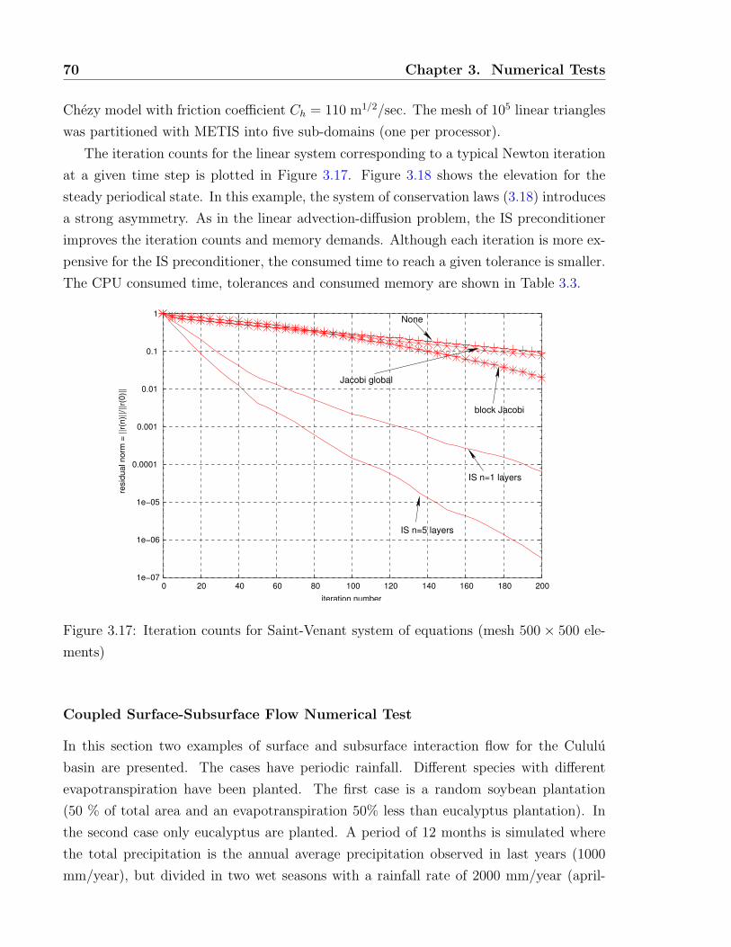
70 Chapter 3. Numerical Tests
Chezy model with friction coefficient Ch = 110 m1/2/sec. The mesh of 105 linear triangles
was partitioned with METIS into five sub-domains (one per processor).
The iteration counts for the linear system corresponding to a typical Newton iteration
at a given time step is plotted in Figure 3.17. Figure 3.18 shows the elevation for the
steady periodical state. In this example, the system of conservation laws (3.18) introduces
a strong asymmetry. As in the linear advection-diffusion problem, the IS preconditioner
improves the iteration counts and memory demands. Although each iteration is more ex-
pensive for the IS preconditioner, the consumed time to reach a given tolerance is smaller.
The CPU consumed time, tolerances and consumed memory are shown in Table 3.3.
1e−07
1e−06
1e−05
0.0001
0.001
0.01
0.1
1
0 20 40 60 80 100 120 140 160 180 200
resi
dual
nor
m =
||r(
n)||/
||r(0
)||
iteration number
IS n=5 layers
IS n=1 layers
block Jacobi
None
Jacobi global
Figure 3.17: Iteration counts for Saint-Venant system of equations (mesh 500 × 500 ele-
ments)
Coupled Surface-Subsurface Flow Numerical Test
In this section two examples of surface and subsurface interaction flow for the Cululu
basin are presented. The cases have periodic rainfall. Different species with different
evapotranspiration have been planted. The first case is a random soybean plantation
(50 % of total area and an evapotranspiration 50% less than eucalyptus plantation). In
the second case only eucalyptus are planted. A period of 12 months is simulated where
the total precipitation is the annual average precipitation observed in last years (1000
mm/year), but divided in two wet seasons with a rainfall rate of 2000 mm/year (april-

3.2. Numerical Examples in Parallel Environment 71
Figure 3.18: Solution of Saint-Venant system of equations (mesh 500× 500 elements)
Table 3.3: CPU time and memory requirements for Saint-Venant equations (mesh 500×500 elements). Note: * in table means iteration failed to converge to a specified tolerance
in a maximum of 400 its.
Preconditioner none Jacobi glob. block − Jacobi ISP (nlay = 1) ISP (nlay = 5)
factorization [secs] - - 8.1 9.0 9.2
GMRes stage [secs] * * 522 68 43
tolerance 1.e-05 1.e-05 1.e-05 1.e-05 1.e-05
memory/proc. [Mb] * * 605 548 550

72 Chapter 3. Numerical Tests
march and september-october) and dry seasons of 500 mm/year (the rest of the year).
At time t = 0 the piezometric height in the phreatic aquifer is 30 meters above the
aquifer bottom, while the water height in stream is 10 meters above the streambed. The
hydraulic conductivity and storativity of phreatic aquifer are 2 · 10−3 and 2.5 · 10−2 msec
,
respectively. The Manning friction law is adopted for this case. The roughness of stream
channel is 3 · 10−3 and the river width is 10 meters. The stream loss resistivity average
value is 105sec. A mesh of 96131 triangular elements and 48452 nodal points is used
to represent the aquifer domain. The average space between nodal river points is 100
meters. The time step adopted in both cases is Dt = 1 day. Figure 3.19 we can see the
1e−07
1e−06
1e−05
0.0001
0.001
0.01
0.1
1
0 50 100 150 200 250 300 350 400
resi
dual
nor
m =
||r(
n)||/
||r(0
)||
iteration number
IS n=5 layers
IS n=1 layers
Jacobi global
none
Figure 3.19: Iteration counts for the coupled flow
iteration counts for different preconditioners. In Figure 3.21 the correlation between the
presence of soybean and a greater phreatic elevation with respect to the levels observed
in the case where only eucalyptus are present is shown. In Figure 3.22 shows the phreatic
elevation after two years of simulation. The time adopted to solve each time step in the
non-linear coupled problem with six processors Pentium IV 1.4-1.7 Ghz and 512 Mb RAM
(Rambus) connected through a switch Fast Ethernet (100 Mbit/sec, latency=O(100)) was
13.2 seconds in average.

3.2. Numerical Examples in Parallel Environment 73
Figure 3.20: Soybean location
50% soybean − 50% eucalyptus
* only eucalyptus
soybean placement
−3
−2
−1
0
1
2
3
4
−40000 −30000 −20000 −10000 0 10000 20000 30000 40000 50000 60000
phi [
mts
]
x (profile at y=0 mts [north−south])
water level difference in freatic aquifer [mts]
Figure 3.21: Difference in phreatic levels for both cases

74 Chapter 3. Numerical Tests
Figure 3.22: Aquifer State at t=2 years
3.2.4 The Stokes Flow in a Long Horizontal Channel
Note: The cluster architecture for the tests given hereafter is slightly different to the
architecture used for the above tests. The tests were carried out on sixteen (uniprocessor)
nodes Pentium IV - 2.8 GHz, 2 GB RAM (DDR, 400 MHz). The nodes are connected
through a switch Fast Ethernet (100 Mbit/sec, latency=O(100) µsecs, each node has a
3COM 3c509 (Vortex) Nic cards).
Triggered by observed discrepancies between experimental results and computer sim-
ulations [KK03] using standard solvers [SB03] (i.e., GMRes with acceptable rates of con-
vergence), this example shows the improvement of the solution of lubricated contacts by
means of the ISP preconditioner. So far the lubricant flow in the narrow gap between two
contacting elements has been described using the Reynolds equation. This equation fol-
lows from the Navier-Stokes equations at low Reynolds number (Re < 1) when a narrow
gap is assumed (i.e., when e = H/L 1 ifH is the gap width and L a characteristic length
scale). Nominally the assumption e 1 will generally hold. An accurate description of
the flow then requires the use of incompressible laminar Navier-Stokes model.

3.2. Numerical Examples in Parallel Environment 75
Incompressible Navier-Stokes Equations
The incompressible Navier-Stokes equations present two important difficulties for solving
it with finite elements. First, the character of the equation becomes highly advective
dominant when the Reynolds number increases. In addition, the incompressibility con-
dition does not represent an evolution equation but a constraint on the equations. This
is a drawback because only some combination of interpolation spaces for velocity and
pressure can be used with the Galerkin formulation, namely those ones that satisfy the
so-called Ladyzhenskaya-Brezzi-Babuska condition. In the formulation of Tezduyar et al.
advection is stabilized with the well known SUPG stabilization term, and a similar stabi-
lization term called PSPG is included in order to stabilize incompressibility. In this way, it
is possible to use stable equal order interpolations. Once these equations are discretized,
the resulting system of ODE’s is discretized in time with the standard trapezoidal rule
(backward Euler and Crank-Nicolson schemes are allowed to be used). The resulting
non-linear system of equation is solved iteratively at every time step. Viscous flow is
Figure 3.23: Olga Alexandrovna Ladyzhenskaya (1922–2004)
well represented by Navier-Stokes equations. The incompressible version of this model
includes the mass and momentum balances that can be written in the following form. Let
Ω ∈ Rnsd and (0, t+] be the spatial and temporal domains respectively, where nsd is the
number of space dimensions, and let Γ be the boundary of Ω. Thus, the equations are
∇ · u = 0 in Ω× (0, t+]
ρ(∂u
∂t+ u · ∇u)−∇ · σ = 0 in Ω× (0, t+],
(3.30)

76 Chapter 3. Numerical Tests
Figure 3.24: Phyllis Nicolson (1917–1968)
Figure 3.25: John Crank (1916–)
with ρ and u the density and velocity of the fluid and σ the stress tensor, given by
σ = −pI + 2µ∗ε(u)
ε(u) = 1/2(∇u + (∇u)t),(3.31)
where p is the pressure and µ∗ is the effective dynamic viscosity defined as sum of the
dynamic (molecular) viscosity and the algebraic eddy viscosity of the LES model proposed
by Smagorinsky [Sma63], i.e., µ∗ = µ+ µSGS. Here I represents the identity tensor and ε
the strain rate tensor.

3.2. Numerical Examples in Parallel Environment 77
The initial and boundary conditions are
Γ = Γg ∪ Γh
Γg ∩ Γh = ∅
u = g at Γg
n · σ = h at Γh,
u(t = 0) = u0 ∀x ∈ Ω
p(t = 0) = p0 ∀x ∈ Ω,
(3.32)
where Γg and Γh are the Dirichlet and Neumann boundaries, respectively. When the flow
velocity is very small (i.e., the fluid is very viscous) or the geometric dimensions are very
small, that is when Reynolds number is very small, the inertial term in (3.30) plays a
minor role and the flow is dominated by the viscous and the pressure gradient terms.
This is the so-called ‘Stokes flow’.
Spatial Discretization. The spatial discretization has equal order for pressure and ve-
locity and is stabilized through the addition of two operators. Advection at high Reynolds
numbers is stabilized with the well known SUPG operator, while the PSPG operator pro-
posed by Tezduyar et al. [TMRS92] stabilizes the incompressibility condition, which is
responsible of the checkerboard pressure modes.
The computational domain Ω is divided in nel finite elements Ωe, e = 1, . . . , nel, and
let E be the set of these elements, and H1h the finite dimensional space defined by
H1h =φh|φh ∈ C0(Ω), φh|Ωe ∈ P 1,∀Ωe ∈ E
, (3.33)
with P 1 representing polynomials of first order. The functional spaces for the interpolation
and weight functions are defined as
Shu = uh|uh ∈ (H1h)nsd ,uh=gh on Γg
V hu = wh|wh ∈ (H1h)nsd ,wh=0 on Γg
Shp = q|q ∈ H1h .
(3.34)

78 Chapter 3. Numerical Tests
The SUPG-PSPG scheme is written as follows: Find uh ∈ Shu and ph ∈ Sh
p such that∫Ω
wh · ρ(∂uh
∂t+ uh · ∇uh
)+
∫Ω
ε(wh) : σhdΩ+
+
nel∑e=1
∫Ω
δh ·[ρ(∂uh
∂t+ uh · ∇uh)−∇ · σh
]︸ ︷︷ ︸
(SUPG term)
+
+
nel∑e=1
∫Ω
εh ·[ρ(∂uh
∂t+ uh · ∇uh)−∇ · σh
]︸ ︷︷ ︸
(PSPG term)
+
+
∫Ω
qh∇ · uhdΩ =
∫Γh
wh · hhdΓ, ∀wh ∈ V hu , ∀qh ∈ Sh
p ,
(3.35)
where the stabilization parameters in equation (3.35) are defined as
δh = τSUPG(uh · ∇)wh
εh = τPSPG1
ρ∇qh
τPSPG = τSUPG =helem
2||uh||z(Reu).
(3.36)
Note that the SUPG and the PSPG terms are defined on different functional spaces.
These stabilizations terms act, at the linear system level, adding nonzero values on the
diagonal entries associated with the pressure equations. The Reynolds number Reu based
on the element parameters is
Reu =||uh||helem
2ν, (3.37)
and the element size helem is computed as,
helem = 2( nn∑
a=1
|s · ∇Na|)−1
, (3.38)
Na being the shape function associated with the node a, nn the number of nodes in the
element, and s a unit vector on the streamline direction. The function z(Re) is defined
as
z(Re) =
Re/3 0 ≤ Re < 3
1 3 ≤ Re.(3.39)
Test and Results
The channel is 8 · 10−5m width and 9 · 10−2m long. The dynamic viscosity used is 5.33 ·10−4m2/sec and no body forces are considered. The Reynolds number based on the
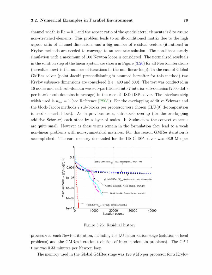
3.2. Numerical Examples in Parallel Environment 79
channel width is Re = 0.1 and the aspect ratio of the quadrilateral elements is 5 to assure
non-stretched elements. This problem leads to an ill-conditioned matrix due to the high
aspect ratio of channel dimensions and a big number of residual vectors (iterations) in
Krylov methods are needed to converge to an accurate solution. The non-linear steady
simulation with a maximum of 100 Newton loops is considered. The normalized residuals
in the solution step of the linear system are shown in Figure (3.26) for all Newton iterations
(hereafter nnwt is the number of iterations in the non-linear loop). In the case of Global
GMRes solver (point Jacobi preconditioning is assumed hereafter for this method) two
Krylov subspace dimensions are considered (i.e., 400 and 800). The test was conducted in
16 nodes and each sub-domain was sub-partitioned into 7 interior sub-domains (2000 dof’s
per interior sub-domains in average) in the case of IISD+ISP solver. The interface strip
width used is nlay = 1 (see Reference [PS05]). For the overlapping additive Schwarz and
the block-Jacobi methods 7 sub-blocks per processor were chosen (ILU(0) decomposition
is used on each block). As in previous tests, sub-blocks overlap (for the overlapping
additive Schwarz) each other by a layer of nodes. In Stokes flow the convective terms
are quite small. However as these terms remain in the formulation they lead to a weak
non-linear problems with non-symmetrical matrices. For this reason GMRes iteration is
accomplished. The core memory demanded for the IISD+ISP solver was 48.9 Mb per
0 10000 20000 30000 400001e−11
1e−09
1e−07
1e−05
0.001
0.1
1
Iteration counts
resi
dual
nor
m =
||r(
n)||/
||r(0
)||
IISD+ISP / nlay
=1 / 7 sub−domains / nnwt=2
Additive Schwarz / 7 sub−blocks / nnwt=20
Block Jacobi / 7 sub−blocks / nnwt=22
global GMRes / Kdim
=800 / Jacobi prec. / nnwt=100
global GMRes / Kdim
=400 / Jacobi prec. / nnwt=100
Figure 3.26: Residual history
processor at each Newton iteration, including the LU factorization stage (solution of local
problems) and the GMRes iteration (solution of inter-subdomain problems). The CPU
time was 0.33 minutes per Newton loop.
The memory used in the Global GMRes stage was 126.9 Mb per processor for a Krylov

80 Chapter 3. Numerical Tests
subspace dimension (KSPdim) of 800 and 63.2 Mb per processor for a KSPdim of 400. The
CPU time was 6.61 minutes and 1.87 minutes per Newton iteration, respectively.
For the overlapping additive Schwarz preconditioning the consumed memory and the
CPU time per Newton iteration were 107 Mb and 1.1 minutes, respectively. Block-Jacobi
scheme consumed 99.3 Mb and 0.97 minutes per non-linear iteration.
In Figures (3.27), (3.28), (3.29) and (3.30) the numerical solution of the horizontal
velocity and pressure fields are compared to the analytical one. Figures (3.27) and (3.28)
correspond to the solution of both fields after one loop in the Newton scheme and Fig-
ures (3.29) and (3.30) correspond to one hundred iterations in Newton’s loop for the
preconditioned Global GMRes method (20 and 22 iterations for additive Schwarz and
block-Jacobi schemes, respectively). For the IISD+ISP solver the residual of the Newton
loop after three iterations was 10−14 and we consider that there is no need to go further
in this loop to converge to the solution. The same residual tolerance was obtained by ad-
ditive Schwarz and block-Jacobi preconditioned on the 20th and 22nd loops, respectively.
Clearly, in this case IISD+ISP outperforms other domain decomposition techniques not
only in memory and CPU time demands but also in the number of non-linear iterations
to achieve a given tolerance. Figures 3.27 and 3.29 show a slight loss in momentum due
0 2 4 6 8x 10
−5
0
0.2
0.4
0.6
0.8
1
y−coordinate [m]
x−ve
loci
ty [m
/sec
]
global GMRes Kdim
=400/Jacobi prec.global GMRes K
dim=800/Jacobi prec.
IISD+ISP nlay
=1
Additive Schwarz/7 sub−blocksBlock Jacobi prec./7 sub−blocksanalytical solution
Figure 3.27: Velocity field in the channel height (nnwt=1)
to the coarse discretization in the transversal direction in order to maintain the aspect
ratio of the elements.
This example was the first evidence that has inspired the article published in [PNS06].
It shows that for high aspect ratio geometries the Global GMRes suffers of a strong

3.2. Numerical Examples in Parallel Environment 81
0 0.02 0.04 0.06 0.08 0.10
1
2
3
4
5
6x 10
4
y−coordinate [m]
Pre
ssur
e [P
a]
global GMRes Kdim
=400/Jacobi prec.global GMRes K
dim=800/Jacobi prec.
IISD+ISP nlay
=1
Additive Schwarz/7 sub−blocksBlock Jacobi prec./7 sub−blocksanalytical solution
Figure 3.28: Pressure field along channel (nnwt=1)
0 2 4 6 8x 10
−5
0
0.5
1
1.5
y−coordinate [m]
x−ve
loci
ty [m
/sec
]
global GMRes Kdim
=400/Jacobi prec./nnwt=100global GMRes K
dim=800/Jacobi prec./nnwt=100
IISD+ISP nlay
=1/nnwt=3
Additive Schwarz/7 sub−blocks/nnwt=20Block Jacobi prec./7 sub−blocks/nnwt=22analytical solution
Figure 3.29: Velocity field in the channel height (nnwt=100 for Global GMRes, nnwt=3
for IISD+ISP, nnwt=20 for additive Schwarz, nnwt=22 for block-Jacobi)
convergence deterioration and even though using an unusually high size of Krylov subspace
dimension the final solution is unacceptable.

82 Chapter 3. Numerical Tests
0 0.02 0.04 0.06 0.08 0.10
1
2
3
4
5
6
7
8
x 104
y−coordinate [m]
Pre
ssur
e [P
a]
global GMRes Kdim
=400/Jacobi prec./nnwt=100global GMRes K
dim=800/Jacobi prec./nnwt=100
IISD+ISP nlay
=1/nnwt=3
Additive Schwarz/7 sub−blocks/nnwt=20Block Jacobi prec./7 sub−blocks/nnwt=22analytical solution
Figure 3.30: Pressure field along channel (nnwt=100 for Global GMRes, nnwt=3 for
IISD+ISP, nnwt=20 for additive Schwarz, nnwt=22 for block-Jacobi)
3.2.5 The Viscous Incompressible Navier-Stokes Flow Around
an Infinite Cylinder
The unsteady viscous external flows past objects have been extensively studied (experi-
mentally and numerically, see References [BCHM86, Cho73, ST90, BLST90, Ros54, Wil85,
Nor01]) because of their many practical applications. For example, airfoils have stream-
line shapes in order to increase the lift and reduce the aerodynamic drag exerted on the
wings at the same time. Another example is the flow past a blunt body, such as a cir-
cular cylinder (e.g., the wind forces acting on the tensors of a hanging bridge), usually
experiences boundary layer separation and very strong flow oscillations in the wake region
behind the body. This example is directly related to a great number of problems. In cer-
tain Reynolds number range, a periodic flow motion will develop in the wake as a result of
the boundary layer vortex being shed alternatively from either side of the cylinder. This
regular pattern of vortices in the wake is called the von-Karman vortex street. It creates
an oscillating flow at a discrete frequency that is correlated to the Reynolds number of
the flow. The periodic nature of the vortex shedding phenomenon can sometimes lead
to unwanted structural vibrations, especially when the shedding frequency matches one
of the resonant frequencies of the structure. In order to generate vortex shedding, an
artificial perturbation may be imposed introducing for example a rotation of the cylinder
for a short time. The perturbations introduced correspond to a clockwise rotation of the
cylinder followed by a counterclockwise rotation (it is of the same nature as the pertur-
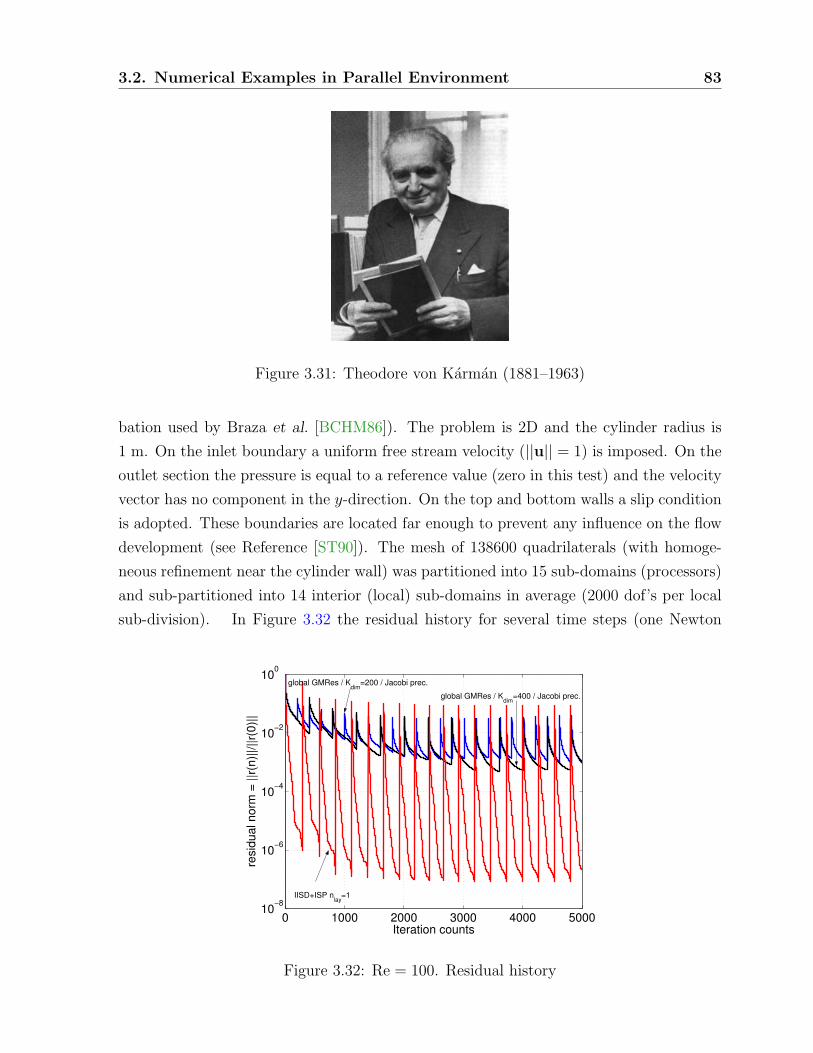
3.2. Numerical Examples in Parallel Environment 83
Figure 3.31: Theodore von Karman (1881–1963)
bation used by Braza et al. [BCHM86]). The problem is 2D and the cylinder radius is
1 m. On the inlet boundary a uniform free stream velocity (||u|| = 1) is imposed. On the
outlet section the pressure is equal to a reference value (zero in this test) and the velocity
vector has no component in the y-direction. On the top and bottom walls a slip condition
is adopted. These boundaries are located far enough to prevent any influence on the flow
development (see Reference [ST90]). The mesh of 138600 quadrilaterals (with homoge-
neous refinement near the cylinder wall) was partitioned into 15 sub-domains (processors)
and sub-partitioned into 14 interior (local) sub-domains in average (2000 dof’s per local
sub-division). In Figure 3.32 the residual history for several time steps (one Newton
0 1000 2000 3000 4000 500010
−8
10−6
10−4
10−2
100
Iteration counts
resi
dual
nor
m =
||r(
n)||/
||r(0
)||
IISD+ISP nlay
=1
global GMRes / Kdim
=200 / Jacobi prec.
global GMRes / Kdim
=400 / Jacobi prec.
Figure 3.32: Re = 100. Residual history

84 Chapter 3. Numerical Tests
iteration is considered) is plotted for the unsteady simulation of this flow. Clearly, the
IISD+ISP solver reaches the lower residual tolerances (10−7 vs 10−3) with 70 % less iter-
ations (roughly) compared to Global GMRes iteration with different KSPdim. The lower
tolerances achieved with IISD+ISP are directly related to the accuracy in the solution
and the reduction of the iteration number influences the overall simulation time. In
0 50 100 150−0.35
−0.345
−0.34
−0.335
−0.33
−0.325
−0.32
−0.315
−0.31
−0.305
Time [secs]
CD
visc
global GMRes / Kdim
=200 / Jacobi prec.
global GMRes / Kdim
=400 / Jacobi prec.
IISD+ISP / nlay
=1
Figure 3.33: Re = 100. viscous x-force coefficient
0 50 100 150−0.06
−0.04
−0.02
0
0.02
0.04
0.06
Time [secs]
CLv
isc
global GMRes / Kdim
=400 / Jacobi prec.
global GMRes / Kdim
=200 / Jacobi prec. IISD+ISP / n
lay=1
Figure 3.34: Re = 100. viscous y-force coefficient
Figures 3.33, 3.34 and 3.35 the viscous forces and moment evolution in time are shown.
The solution obtained with both Global Iteration (KSPdim = 400) and IISD+ISP are in
agreement with the experimental results reported by Braza et al., and with the numerical

3.2. Numerical Examples in Parallel Environment 85
0 50 100 150−8
−6
−4
−2
0
2
4
6x 10⁻³
Time [secs]
z−m
omen
t visc
global GMRes / Kdim
=400 / Jacobi prec.
global GMRes / Kdim
=200 / Jacobi prec.
IISD+ISP / nlay
=1
Figure 3.35: Re = 100. viscous z-moment coefficient
results shown in References ([BCHM86, ST90, BLST90]). However, if Global Iteration
is stopped prematurely (i.e., KSPdim = 200, see Figure 3.32) the solution is no more
accurate and divergences of 50% are observed (see Figure 3.35). Although the residuals
are lowered between two and three orders of magnitude the error in the solution of the
linear system is not accurate enough. Remember that to pass from 200 iterations to 400
iterations in a GMRes scheme the computational resources (CPU and consumed memory)
are considerably increased due to the storage requirements for the Krylov subspace bases.
The CPU consumed time and core memory requirements for each time step were: 28
secs and 100 Mbytes for Global GMRes with KSPdim = 200, 107.5 secs and 152 Mbytes
for Global GMRes with KSPdim = 400 and 18.5 secs and 98 Mbytes for IISD+ISP. The
vorticity field for the LES flow around a 3D cylinder at Re = 5 · 104 is shown in Fig-
ure 3.36. This well known test case shows the need to use Global GMRes with a high
Krylov subspace dimension size to reach the accuracy of IISD+ISP solver. Usually, the
user is pushed to adopt a small value of Krylov subspace dimension in order to reduce
memory and CPU time consumed. The sensitivity of the results obtained using Global
GMRes to the Krylov subspace dimension size is high, and with no a priori knowledge
of this dimension the uncertainties in the results tend to be high. In summary, Global
GMRes iteration makes the simulation more user dependent.

86 Chapter 3. Numerical Tests
Figure 3.36: 3D LES flow at Re = 5 · 104. Top: initial state, bottom: pseudo-stationary
state
3.2.6 Navier-Stokes Flow Using the Fractional Step Scheme.
The Lid Driven Cavity
A test of the disaggregated method was performed on two-dimensional unit cavity flow
at Re = 1000. This is a test that has been computed extensively in the past and it is well
understood (see Reference [GGS82] for a detailed description of this example).

3.2. Numerical Examples in Parallel Environment 87
Disaggregated Scheme
Fractional step methods for the incompressible Navier-Stokes equations have been popular
over the last two decades. The reason for this relies on the computational efficiency of
these methods, basically because of the uncoupling of the pressure from the velocity
components. In Reference [Cod01] the study of computed pressure stability of schemes
that use a pressure Poisson equation was presented. These results are used in this section.
The results to be presented refer to second-order algorithm based on the implicit
(θ = 1) discretization for the viscous and convective terms and a second-order pressure
splitting, leaving the pressure gradient at a given time level in the first step and computing
its increment in the second one.
The time discretization of the problem (3.30) written in a compact matrix form is
M1
∆t(Un+1 −Un) + K(Un+θ)Un+θ + GPn+1 = Fn+θ, (3.40)
DUn+1 = 0, (3.41)
where M is the mass matrix, U is the vector of velocity unknowns, K is the stiffness
matrix, G is the matrix form of the gradient operator, P is the vector of nodal pressures,
D is the matrix form of the divergence operator and F is the vector of source terms.
Superscripts n and n+1 denote variables at time t = n∆t and t = (n+1)∆t, respectively.
The fractional step scheme applied to the fully discrete problem (3.40) and (3.41) is
exactly equivalent to
M1
∆t(Un+1 −Un) + K(Un+θ)Un+θ + γGPn = Fn+θ (3.42)
M1
∆t(Un+1 − Un+1) + G(Pn+1 − γPn) = 0, (3.43)
DUn+1 = 0, (3.44)
where Un+1 is an auxiliary variable and γ is a numerical parameter, whose values of in-
terest are between 0 and 1. The essential approximation K(Un+θ)Un+θ ∼ K(Un+θ)Un+θ
is made, where Un+θ = θUn+1 + (1− θ)Un. Writing Un+1 in terms of Un+1 using (3.43)
and inserting the result in (3.44), the equations to be solved are
M1
∆t(Un+1 −Un) + K(Un+θ)Un+θ + γGPn = Fn+θ, (3.45)
∆tDM−1G(Pn+1 − γPn) = DUn+1, (3.46)
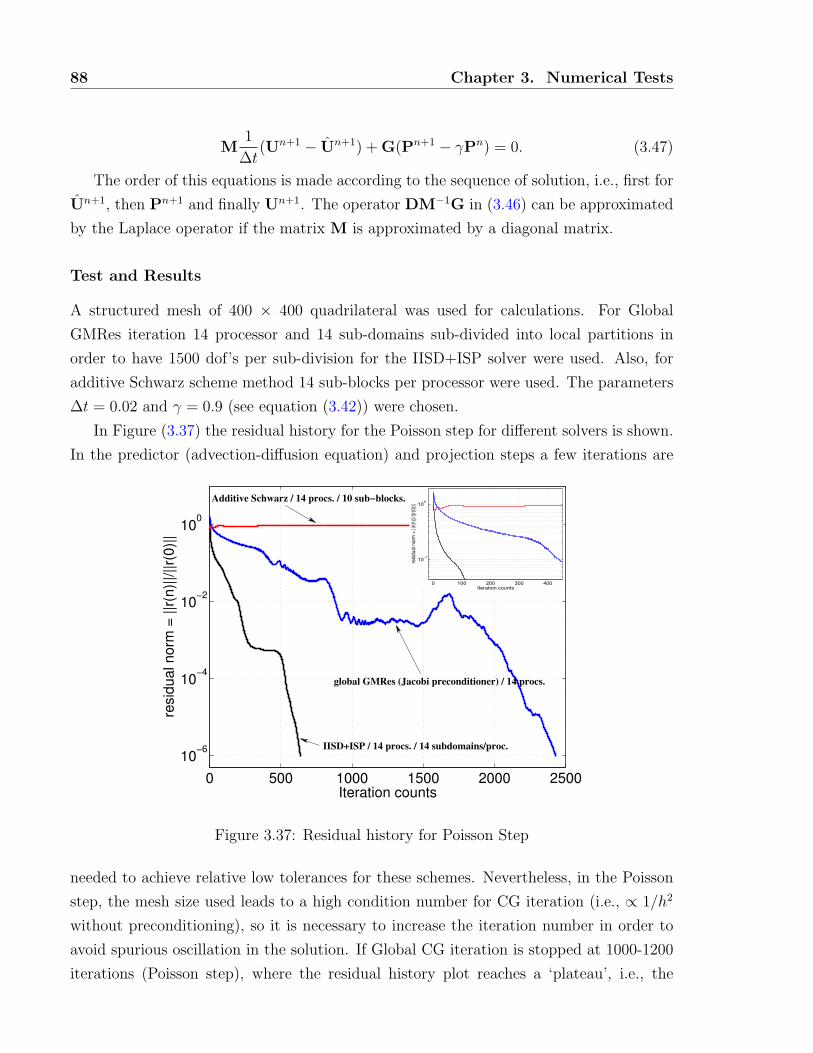
88 Chapter 3. Numerical Tests
M1
∆t(Un+1 − Un+1) + G(Pn+1 − γPn) = 0. (3.47)
The order of this equations is made according to the sequence of solution, i.e., first for
Un+1, then Pn+1 and finally Un+1. The operator DM−1G in (3.46) can be approximated
by the Laplace operator if the matrix M is approximated by a diagonal matrix.
Test and Results
A structured mesh of 400 × 400 quadrilateral was used for calculations. For Global
GMRes iteration 14 processor and 14 sub-domains sub-divided into local partitions in
order to have 1500 dof’s per sub-division for the IISD+ISP solver were used. Also, for
additive Schwarz scheme method 14 sub-blocks per processor were used. The parameters
∆t = 0.02 and γ = 0.9 (see equation (3.42)) were chosen.
In Figure (3.37) the residual history for the Poisson step for different solvers is shown.
In the predictor (advection-diffusion equation) and projection steps a few iterations are
0 500 1000 1500 2000 250010−6
10−4
10−2
100
Iteration counts
resid
ual n
orm
= ||
r(n)||
/||r(0
)||
0 100 200 300 400
10−1
100
Iteration counts
resid
ual n
orm
= ||r
(n)||
/||r(0
)||
IISD+ISP / 14 procs. / 14 subdomains/proc.
global GMRes (Jacobi preconditioner) / 14 procs.
Additive Schwarz / 14 procs. / 10 sub−blocks.
Figure 3.37: Residual history for Poisson Step
needed to achieve relative low tolerances for these schemes. Nevertheless, in the Poisson
step, the mesh size used leads to a high condition number for CG iteration (i.e., ∝ 1/h2
without preconditioning), so it is necessary to increase the iteration number in order to
avoid spurious oscillation in the solution. If Global CG iteration is stopped at 1000-1200
iterations (Poisson step), where the residual history plot reaches a ‘plateau’, i.e., the

3.2. Numerical Examples in Parallel Environment 89
residuals may be considered acceptable, large spurious oscillations appear in the solution
when the steady state is reached. Moreover, it is necessary to overpass the 2400 iterations
to avoid oscillation in all time steps. Although the required memory is not affected
(please recall that in CG iteration, only the last two residual vectors are needed), but the
CPU time grows linearly with the iterations. Using IISD+ISP the amount of memory
to solve the interior direct problem and the preconditioning is chosen (1500 dof’s where
considered for each interior sub-division). The residuals reach low tolerances with few
iterations and the CPU time required for each time step is diminished (although the
local and interface problems are solved). Moreover, it is not necessary to iterate over
the 50 iterations to obtain accurate solutions. Figure (3.38) shows the steady-converged
solution stopping when the iteration reaches 50 using IISD+ISP. The total CPU time
consumed in average for each time step (i.e., predictor, pressure and projection steps)
for Global Iteration (GMRes in predictor step, CG in Poisson and projection step) was
23.61 seconds and for IISD+ISP (with one layer around the interface) solver was 2.13 secs.
Additive Schwarz scheme shows a poor convergence in residuals but it is not necessary to
go beyond 200 iterations to have an acceptable solution. This last scheme uses 26 secs
per time step. The reader could refer to reference [PS05] for a study of the performance
of several preconditioners (including IISD+ISP and Neumann-Neumann preconditioners)
applied to a Poisson’s problem.
Although the residuals for IISD+ISP simulation are higher than those of 1000 iter-
ations of Global CG (see Figure (3.37)), the solution for domain decomposition method
and preconditioning (IISD+ISP) is accurate enough, being oscillatory for Global Iteration.
This behavior can be explained through a study of the error in residuals when iteration
proceeds.
Let b, uk, u0 ∈ RN , A a non-singular matrix such that u∗ = A−1b. Here b is the load
vector and uk the solution at iteration k. Since
rk = b− Auk = Au∗ − Auk = A(uk − u∗) = −Aek, (3.48)
where e is the error in the solution u at the iteration k. Then,
‖ek‖ =∥∥A−1Aek
∥∥ ≤ ∥∥A−1∥∥ ‖Aek‖ =
∥∥A−1∥∥ ‖rk‖ , (3.49)
and
‖r0‖ ≤ ‖A‖ ‖e0‖ , (3.50)
thus,‖ek‖‖e0‖
≤ ‖A−1‖ ‖rk‖‖A‖−1 ‖r0‖
= κ(A)‖rk‖‖r0‖
, (3.51)

90 Chapter 3. Numerical Tests
where κ(A) is the condition number of A and ‖.‖ is any suitable norm. The division by
‖r0‖ and ‖e0‖ in equation (3.51) normalizes the residuals. In Reference [SDP+03] it is
shown that the condition number is κ(A) ∝ O(1/h2) for Global Iteration and κ(A) ∝O(1/h) for Schur complement domain decomposition methods. Moreover, the IISD+ISP
still reduces the last condition number. Though the error in residuals for IISD+ISP (due
to earlier stopping) is higher than the error in residuals for CG at high iteration count, the
factor that determines the error in the solution (xk) is the distribution of the eigenvalues
of the global matrix and its condition number κ (see equation (3.51)). If the solution of
the Poisson step is not accurate, the error is propagated to the other steps and oscillation
may occur. This problem is stressed with the refinement (i.e., h → 0). The primary
0
0.2
0.4
0.6
0.8
1
-0.4 -0.2 0 0.2 0.4 0.6 0.8 1
y-co
ordi
nate
[m]
x-velocity [m/sec]
Ghia et al.
IISD+ISP Krylov dim.=50
Figure 3.38: Time-converged solution for IISD+ISP solver (Re = 1000)
vortex center was computed to be at (x, y) = (0.531, 0.562) with the coordinate reference
system placed at the bottom left corner of the cavity. IISD+ISP solver compares well
(for the 50 iteration run) with the values reported by Ghia et al. The core memory
used was 45 Mbytes/processor for Global Iteration, 60 Mbytes/processor for IISD+ISP
and 55 Mbytes/processor for the additive Schwarz preconditioner. Recalling that for CG
iteration only the last two residuals are needed, then the memory is not increased with
iterations.
This example allows to emphasize another interesting use of IISD+ISP solver. In
fractional step-like flow solvers the Poisson step has normally the higher CPU time con-

3.2. Numerical Examples in Parallel Environment 91
sumption and for ill-conditioned problems this step demands a lot of resources to achieve
a good solution. It is difficult to know right from the start how large the Krylov sub-
space dimension size of conjugate gradient method has to be and this example shows its
strong influence on the final solution. Moreover, with an unusually high Krylov subspace
dimension of 1000-1500, the solution of lid driven square cavity is already unacceptable
making its usage too limited. With IISD+ISP it is possible to strongly reduce these re-
quirements and this fact drastically improves the solution and makes the system solution
less user-dependent.
Some Comments on the Scalability of the IISD+ISP Preconditioner
In article [PS05] the condition number for the preconditioned Poisson and Advection-
Diffusion problems was calculated theoretically for the Interface Strip preconditioner. In
this section the scalability of the Interface Strip preconditioner is studied by showing how
the number of iterations grows with the global size of the problem while keeping the size
of the problem in each processor constant. Stokes flow at Re = 0.01 with monolithic time
integration (time step used is ∆t = 0.1) is considered. The square cavity is divided into
(20 ·nproc)×(20 ·nproc) bilinear elements, with nproc being the number of processors. Inside
each processor, the problem is further sub-divided into 4 sub-domains and the number
of element layers around the interface is kept constant to nlay = 1. In Figure (3.39) the
number of iterations to achieve a relative tolerance of 10−8 in the residuals in a given
time step is shown. It may be observed that the number of iterations saturates for an
increasing problem size, ensuring the scalability of the preconditioner.
2 4 6 8 10 120
20
40
60
80
100
120
num
ber o
f ite
ratio
ns
number of processors
Figure 3.39: Scalability properties

92 Chapter 3. Numerical Tests
3.2.7 The Wind Flow Around a 3D Immersed Body.
The AHMED Model
Current vehicle design needs a strong background in aerodynamics to improve flow control
via mechanical devices. The complexity involved in the automobile design, specially due
to the great amount of accessories that define its geometry, makes the validation tasks
unaffordable. The Ahmed model is a simple geometric body that retains the main flow
features, specially the vortex wake flow where most part of the drag is concentrated, and
it is a good candidate to be used as a benchmark test. The flow regime of interest for
car designers is fully turbulent. So, a large eddy simulation (LES) turbulence model is
employed (see References [KD03, Sma63]). The aerodynamic forces on road vehicles are
the result of complex interactions between flow separations and the dynamic behavior
of the released vortex wake. The results obtained with two solvers (i.e., IISD+ISP and
Jacobi preconditioned Global GMRes methods) are compared to the detailed flow patterns
previously published by Ahmed and coworkers [ARF84].
The body geometry is defined in [ARF84]. The flow domain chosen is one in which
the body of length L is suspended to 0.05 m to the ground in a domain of 10L×2L×1.5L
in the stream-wise (y), span-wise (x) and stream-normal (z) directions. The boundary
conditions for this problem are: uniform flow at the inlet (given by the Reynolds number),
slip condition on both sides, non-slip condition for the surface of the body and non-slip
condition at the floor. Imposed pressure (zero in this case) is used at the outflow boundary
condition.
Ahmed Body: Numerical Results for Very Low Reynolds Number
First, consider the steady Stokes flow (solved using incompressible Navier-Stokes model at
Re = 0.1) around the Ahmed body. The inlet (free stream) condition is Re = 0.1 with no
transversal velocity and the pressure, p = 0 atm, is imposed at the outflow wall (located
far enough from the body). In this test a non-structured tetrahedral mesh is used in the
whole flow domain and a three-layer structured mesh of wedge (prismatic) elements is
built for capturing details at the boundary layers. The body surface mesh contains 90606
nodes while the boundary layer mesh has 180600 elements and the tetrahedral mesh has
1322876 elements. The tests were carried out on 15 processors. For IISD+ISP solver 2000
dof’s were considered for each local sub-division.
The residual history for several Newton loops is shown in Figure 3.40. The calculated
forces and moments for both solvers are shown in Figures 3.41 to 3.43. Clearly, IISD+ISP
converges to the steady solution in one Newton iteration whereas Global Iteration needs

3.2. Numerical Examples in Parallel Environment 93
0 1000 2000 3000 4000 5000 6000
10−10
10−8
10−6
10−4
10−2
100
Iteration counts
resid
ual n
orm
= ||
r(n)||
/||r(0
)||
global GMRes (Jacobi preconditioner) / Kdim=300
IISD+ISP / nlay=1
Figure 3.40: Stokes Flow. Residual history (max. of 100 Newton iterations)
0 2 4 6 8 100.3
0.4
0.5
0.6
0.7
0.8
0.9
1
Newton iterations
C D
global GMRes (Jacobi prec.) / Kdim=350
IISD+ISP / nlay=1
0 2 4 6 8 10−7
−6.5
−6
−5.5
−5
−4.5
−4 x 10⁻⁴
Newton iterations
C Y
global GMRes (Jacobi prec.) / Kdim=350
IISD+ISP / nlay=1
Figure 3.41: Stokes Flow. Force and moment coefficients
more iteration counts to achieve convergence. This behavior is directly related to the
CPU time needed to obtain converged solution in a simulation.
The CPU consumed time and core memory requirements (in average) for each Newton
iteration were: 185.1 secs and 443 Mbytes for Global GMRes with KSPdim = 300 and
64.18 secs and 588 Mbytes for IISD+ISP.
Ahmed Body: Numerical Results for High Reynolds Number
In this section the unsteady incompressible Navier-Stokes simulation for the flow around
the Ahmed body for Re = 1000 is shown. The same architecture, mesh and partitions of
the previous example were used. The initial state used is the steady converged solution of

94 Chapter 3. Numerical Tests
0 2 4 6 8 10−0.25
−0.2
−0.15
−0.1
−0.05
0
0.05
0.1
0.15
0.2
Newton iterations
C L
global GMRes (Jacobi prec.) / Kdim=350
IISD+ISP / nlay=1
0 2 4 6 8 10−3
−2.8
−2.6
−2.4
−2.2
−2
−1.8
−1.6
−1.4
−1.2 x 10⁻⁴
Newton iterations
x−m
omen
t coe
fficie
nt
IISD+ISP / nlay=1
global GMRes (Jacobi prec.) / Kdim=350
Figure 3.42: Stokes Flow. Force and moment coefficients
0 2 4 6 8 10−0.2
−0.18
−0.16
−0.14
−0.12
−0.1
−0.08
−0.06
Newton iterations
y−m
omen
t coe
fficie
nt
global GMRes (Jacobi prec.) / Kdim=350
IISD+ISP / nlay=1
0 2 4 6 8 10−5
−4
−3
−2
−1
0
1
2
3 x 10⁻⁴
Newton iterations
z−m
omen
t coe
fficie
nt
global GMRes (Jacobi prec.) / Kdim=350
IISD+ISP / nlay=1
Figure 3.43: Stokes Flow. Force and moment coefficients
the previous example (IISD+ISP case). The Smagorinsky model (with the Smagorinsky
parameter equal to 0.18) is used for the LES prediction of the turbulent effects.
The Residual history for several time steps is shown in Figure 3.44. The calculated
force and moment coefficients for both solvers (Re = 1000.) are shown in Figures 3.45
to 3.47. The scale of the force and moment coefficient plots is dominated by the bad
approximation and oscillations in the solution obtained with the preconditioned Global
GMRes iterations. The calculated forces with IISD+ISP solver converge very fast to the
values reported in the literature [ARF84].
The CPU consumed time and core memory requirements (in average) for time step in
this test were: 186 secs and 460 Mbytes for Global GMRes iteration with KSPdim = 300
and 114.5 secs and 630 Mbytes for the ISD+ISP preconditioner.
The ‘friction lines’ for the Navier-Stokes flow at Re = 4.25 · 106 are shown in fig-

3.2. Numerical Examples in Parallel Environment 95
0 1000 2000 3000 4000 500010−8
10−6
10−4
10−2
100
Iteration counts
resid
ual n
orm
= ||
r(n)||
/||r(0
)||
global GMRes Kdim=300 (Jacobi prec.)IISD+ISP / nlay=1
Figure 3.44: Re = 1000. Residual history (100 time steps, 10 seconds of simulation)
0 10 20 30 40 50 60 70 80 90 100−20
−15
−10
−5
0
5
10
15
20
25
Time steps
C D
global GMRes Kdim=300 (Jacobi prec.)IISD+ISP / nlay=1
0 10 20 30 40 50 60 70 80 90 100−4
−2
0
2
4
6
8
Time steps
C Y
global GMRes Kdim=300 (Jacobi prec.)IISD+ISP / nlay=1
Figure 3.45: Re = 1000. Force and moment coefficients
ure (3.48) (IISD+ISP case). This 3D example shows that even when the final solution
of Global GMRes solver seems to be similar to IISD+ISP, the former needs more time
steps or more Newton iterations to reach the final solution. This fact is highlighted in the
Stokes flow example (Re = 0.1). For medium Reynolds numbers the Global GMRes has
a strong oscillatory behavior until it reaches the good solution, making the scheme under
external perturbations more unstable.
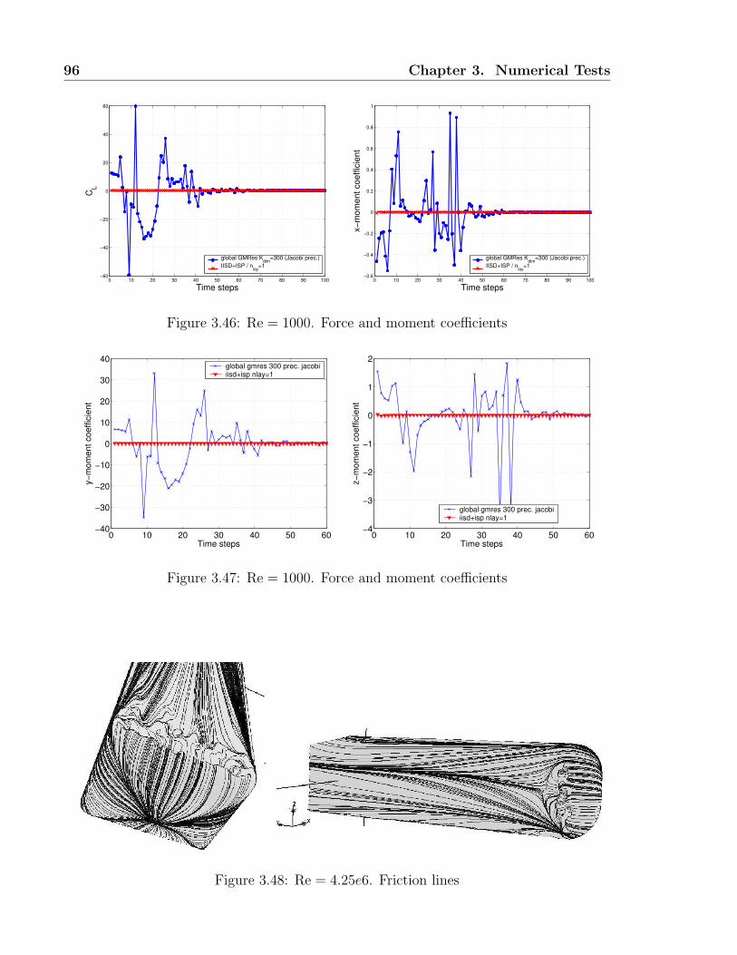
96 Chapter 3. Numerical Tests
0 10 20 30 40 50 60 70 80 90 100−60
−40
−20
0
20
40
60
Time steps
C L
global GMRes Kdim=300 (Jacobi prec.)IISD+ISP / nlay=1
0 10 20 30 40 50 60 70 80 90 100−0.6
−0.4
−0.2
0
0.2
0.4
0.6
0.8
1
Time steps
x−m
omen
t coe
fficie
nt
global GMRes Kdim=300 (Jacobi prec.)IISD+ISP / nlay=1
Figure 3.46: Re = 1000. Force and moment coefficients
0 10 20 30 40 50 60−40
−30
−20
−10
0
10
20
30
40
Time steps
y−m
omen
t coe
ffici
ent
global gmres 300 prec. jacobiiisd+isp nlay=1
0 10 20 30 40 50 60−4
−3
−2
−1
0
1
2
Time steps
z−m
omen
t coe
ffici
ent
global gmres 300 prec. jacobiiisd+isp nlay=1
Figure 3.47: Re = 1000. Force and moment coefficients
Figure 3.48: Re = 4.25e6. Friction lines

3.3. Conclusions 97
3.3 Conclusions
This section emphasizes the quality and the efficiency of solver schemes for CFD problems.
Both criteria should be evaluated together to analyze the performance of a simulation.
Reasonable efficiency might not be very significant if the solution is not accurate enough
for the final purpose. Several examples presented in this section shed light on the patholo-
gies that may appear when solving large scale CFD problems by means of fully iterative
solvers with limited computational resources.
Numerical experiments of several physical (real) problems were carried out to show
their convergence properties, the computation time and memory requirements using both
monolithic and disaggregated schemes. These tests showed that it is not always possible
to obtain an acceptable solution for the problem using classical Global Krylov methods.
Moreover, for some problems Krylov dimension and Newton iterations need to be enlarged
to obtain an accurate solution making its usage more user-dependent.
Domain Decomposition techniques, especially the Schur Complement domain decom-
position using the Interface Strip Preconditioner are suitable in order to achieve accurate
solutions efficiently. In all cases, the performance of IISD+ISP is decisive when it comes
to assigning computational resources to solve a time step in the simulation of a prob-
lem. Also, the ISP preconditioner is easy to construct as it does not require any special
calculation (it can be assembled with a subset of sub-domain matrix coefficients). It is
much less memory-consuming than classical preconditioners such as Neumann-Neumann
as References [SDP+03] and [PS05] shown. Moreover, it permits to decide how much
memory to assign for preconditioning purposes.
The ISP preconditioner is well suited for flows with high Reynolds numbers where
the contribution of advective terms are predominant in the governing equations, while
it is capable to handle diffusion-dominated regions well. Furthermore, IISD+ISP is a
good alternative to treat problems where domain discretization presents high refinement
gradients.


Part II
Applications and Usage
99


Chapter 4
Dynamic Boundary Conditions in
CFD
No one is anyone,
one single immortal man is all men.
Like Cornelius Agrippa,
I am god, I am hero,
I am philosopher, I am demon
and I am world,
which is a tedious way of saying
that I do not exist.
‘The Immortal’, Jorge Luis Borges
The number and type of boundary conditions to be used in the numerical modeling
of fluid mechanics problems is normally chosen according to a simplified analysis of the
characteristics, and also from the experience of the modeler. The problem is harder at
input/output boundaries which are, in most cases, artificial boundaries, so that a bad de-
cision about the boundary conditions to be imposed may affect the precision and stability
of the whole computation. For inviscid flows, the analysis of the sense of propagation
in the normal direction to the boundaries gives the number of conditions to be imposed
101

102 Chapter 4. Dynamic Boundary Conditions in CFD
and, in addition, the conditions that are ‘absorbing’ for the waves impinging normally to
the boundary. In practice, it amounts to counting the number of positive and negative
eigenvalues of the advective flux Jacobian projected onto the normal. The problem is
still harder when the number of incoming characteristics varies during the computation,
and the correct treatment of these cases poses both mathematical and practical problems.
One example considered here is a compressible flow where the flow regime at a certain
part of an inlet/outlet boundary can change from subsonic to supersonic and the flow
can revert. In this chapter the technique for dynamically imposing the correct number of
boundary conditions along the computation, using Lagrange multipliers and penalization,
is discussed and several numerical examples are presented.
4.1 Introduction
Deciding how many and which boundary conditions to impose at each part of an artificial
boundary is often a difficult problem. This decision is taken from the number of incoming
characteristics n+ and the quantities known for each problem. On one hand, if the number
of conditions imposed on the boundary is in excess they are absorbed through spurious
shocks at the boundary. On the other hand if fewer conditions are imposed, then the
problem is mathematically ill posed. Even if the number of imposed boundary conditions
is correct, this does not guarantee that the boundary conditions are non-reflective.
When dealing with models in infinite domains one has to introduce an artificial bound-
ary distant as far as possible from the region of interest. The simplest choice is to impose
a boundary condition assuming that the flow far from the region of interest is undis-
turbed. However, one has the freedom of choosing the boundary condition so as to give
the best solution for a given position of the boundary. Boundary conditions that tend to
give the solution as if the domain were infinite are called generally ‘absorbing’ (ABC) or
‘non-reflective’ (NRBC). ABC’s tend to give a better solution for a given position of the
artificial boundary or, in other words, they allow to put the artificial boundary closer to
the region of interest for a given admissible error. Of course, the advantage of putting the
artificial boundary closer to the region of interest is the reduction in computational cost.
However, in some cases, like for instance the solution of the Helmholtz equation on exte-
rior domains, using absorbing boundary conditions is required since using a non absorbing
boundary condition (like Dirichlet or Neumann) may lead to a lack of convergence of the
problem, because these conditions are completely reflective and therefore wave energy is
trapped in the domain, producing false resonance modes.
There are basically two approaches for the design of ABC’s, global and local. Global

4.1. Introduction 103
boundary conditions are usually more accurate but expensive. In the limit, a global ABC
may reproduce the effect of the whole external problem onto the boundary, i.e., even
maintaining a fixed position of the artificial boundary the ABC may give a convergent
solution while refining the interior mesh. In general these ABC’s are non-local, i.e., its
discrete operator is a dense matrix. Global boundary conditions exist and are popular for
the simpler linear operators, like potential flow problems and frequency domain analysis of
wave problems, like the Helmholtz equations for acoustics or the Maxwell equations[GK90,
GK89, BR92, HH92, SDEI97, Hag87].
The discrete operator for local absorbing boundary conditions is usually sparse but
has a lower order of accuracy and, in general, it is needed to bring the artificial boundary
to infinity while refining meshes in order to make the whole algorithm convergent. These
kinds of ABC’s are popular for more complex non-linear fluid dynamic problems, like
compressible or incompressible, Navier-Stokes equations or the inviscid Euler equations.
An excellent review has been written by Tsynkov [Tsy98].
In order to have an ABC not any n+ conditions must be imposed at the boundary
but exactly those n+ corresponding to the incoming characteristics. This can be deter-
mined through an eigenvalue decomposition problem of the advective flux Jacobian at the
boundary.
In many cases the number of incoming characteristics may change during the compu-
tation, for instance in compressible flow it is common that the flow goes from subsonic
to supersonic in certain parts of the outlet boundary. In 3D this means passing from one
imposed boundary condition to none.
In more complex problems one can go through the whole possible combinations of
regimes: subsonic inlet, supersonic inlet, subsonic outlet, supersonic outlet. A typical
case where this can happen is the free fall of a blunt symmetrical object like an ellipse,
for instance. If the body starts from rest, it will initially accelerate and, depending on
the size and relation between the densities of the body and the surrounding atmosphere
it may reach the supersonic regime. As the body falls, even at subsonic speeds, its angle
of attack tends to increase until eventually it stalls, and then falls towards its rear part,
and repeating the process in a characteristic movement that recalls the fall of tree leaves.
During the falling, the speed of the object varies periodically, accelerating when the angle
of attach is small and the body experiences little drag, and decelerating when the angle of
attack is large. For a supersonic fall the regime may change from supersonic to subsonic
and back during the fall. In addition, if the problem is solved in a system of coordinates
attached to the body, the unperturbed flow may come from every direction relative to
the body’s axis. In this way the regime and direction of the flow at a given point of the
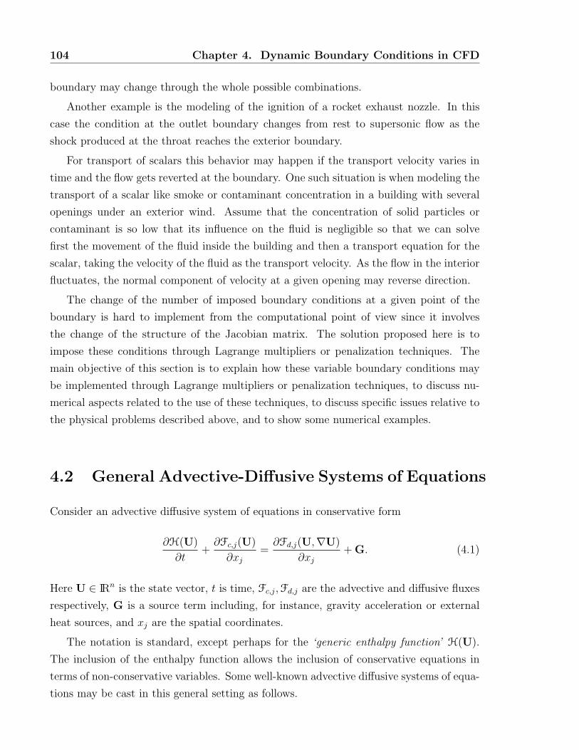
104 Chapter 4. Dynamic Boundary Conditions in CFD
boundary may change through the whole possible combinations.
Another example is the modeling of the ignition of a rocket exhaust nozzle. In this
case the condition at the outlet boundary changes from rest to supersonic flow as the
shock produced at the throat reaches the exterior boundary.
For transport of scalars this behavior may happen if the transport velocity varies in
time and the flow gets reverted at the boundary. One such situation is when modeling the
transport of a scalar like smoke or contaminant concentration in a building with several
openings under an exterior wind. Assume that the concentration of solid particles or
contaminant is so low that its influence on the fluid is negligible so that we can solve
first the movement of the fluid inside the building and then a transport equation for the
scalar, taking the velocity of the fluid as the transport velocity. As the flow in the interior
fluctuates, the normal component of velocity at a given opening may reverse direction.
The change of the number of imposed boundary conditions at a given point of the
boundary is hard to implement from the computational point of view since it involves
the change of the structure of the Jacobian matrix. The solution proposed here is to
impose these conditions through Lagrange multipliers or penalization techniques. The
main objective of this section is to explain how these variable boundary conditions may
be implemented through Lagrange multipliers or penalization techniques, to discuss nu-
merical aspects related to the use of these techniques, to discuss specific issues relative to
the physical problems described above, and to show some numerical examples.
4.2 General Advective-Diffusive Systems of Equations
Consider an advective diffusive system of equations in conservative form
∂H(U)
∂t+∂Fc,j(U)
∂xj
=∂Fd,j(U,∇U)
∂xj
+ G. (4.1)
Here U ∈ IRn is the state vector, t is time, Fc,j,Fd,j are the advective and diffusive fluxes
respectively, G is a source term including, for instance, gravity acceleration or external
heat sources, and xj are the spatial coordinates.
The notation is standard, except perhaps for the ‘generic enthalpy function’ H(U).
The inclusion of the enthalpy function allows the inclusion of conservative equations in
terms of non-conservative variables. Some well-known advective diffusive systems of equa-
tions may be cast in this general setting as follows.

4.2. General Advective-Diffusive Systems of Equations 105
4.2.1 Linear Advection-Diffusion Model
For instance, the heat advection-diffusion equation in terms of temperature can be put in
this form through the definitions
U = T,
H(U) = ρCpT.
Fc,j(U) = ρCpTuj,
Fd,j(U,∇U) = −qj = −k ∂T∂xj
,
(4.2)
where ρ is the density, Cp the specific heat, u a given velocity field, T is the temperature
(the unknown field), q the heat flux vector and k the thermal conductivity of the medium.
4.2.2 Gas Dynamic Equations
Gas dynamic equations of a compressible flow can be put in conservative form with the
following definitions
Up = [ρ,u, p]T ,
U = Uc = [ρ, ρu, ρe]T ,
H(U) = U,
Fc,jnj =
ρ(u · n)
ρu(u · n) + pn
(ρe+ p)(u · n)
,
Fd,j(U,∇U)nj =
0,
T · nTikukni − qini
.
(4.3)
Note that even if the equations are put in terms of conservative variables, the diffusive
and convective fluxes are expressed in term of the primitive variables Up = [ρ,u, p]T .
However, the fluxes can be thought as implicitly depending on the conservative variables,
since the relation Uc(U) is one to one. Now, the conservation equations can be also
thought in terms of any other set of variables, for instance the primitive variables, if we
introduce the ‘enthalpy function’ H(Up) = Uc(Up).

106 Chapter 4. Dynamic Boundary Conditions in CFD
4.2.3 Shallow Water Equations
Shallow water equations describes the open flow of fluids over regions whose characteristic
dimensions are much larger than the depth. In this case
Up = [h,u]T ,
U = Uc = [h, hu]T ,
H(U) = U,
Fc,jnj =
[h(u · n)
h(u · n)u + 1/2gh2 I
],
(4.4)
where h is the fluid depth, u the velocity vector, Up,Uc the primitive and conservative
variables and g the gravity acceleration. We assume that the height of the bottom with
respect to a fixed datum is constant. If this is not so, additional terms must be included
in the source term G, but this is irrelevant for the absorbing boundary condition issue.
4.2.4 Channel Flow
Flow in a channel can be cast in advective form as follows
Up = [h, u]T ,
U = Uc = [A,Q]T ,
H(U) = U,
F =
[Q
Q2/A+ F
],
(4.5)
where h and u are water depth and velocity (as in the shallow water equations). Here
A(h) is the section of the channel occupied by water for a given water height h and then
defines the geometry of the channel. For instance
• Rectangular channels: A(h) = wh, w=width.
• Triangular channels: A(h) = 2h2 tan θ/2; with θ=angle opening.
• Circular channel:
A(h) =
∫ h
h′=0
√2Rh− h2 dh
= θR2 − w(h)(R− h)/2
(4.6)
where R is the radius of the channel, w(h) = 2√
2Rh− h2 is the waterline for a
given water height and θ = atan[w/(2(R− h))] is the angular aperture.

4.3. Variational Formulation 107
The variable Q = Au is the water flow rate and F (h) is a function defined by
F (h) =
∫ h
h′=0
A(h′) dh′. (4.7)
Again, for the sake of simplicity, we restrict the analysis to the case of constant channel
section and channel depth. For more general situations, other terms that can be included
in the source and diffusive terms are present, not needed for the discussion of absorbing
boundary conditions. For rectangular channels the equations reduce to those for one
dimensional shallow water equations. Channel flow is very interesting since it is in fact a
family of different 1D hyperbolic systems depending on the area function A(h).
Figure 4.1 shows the absorption of an initial perturbation in the water height when
the two resulting impinging waves reach the artificial boundaries. The Figure shows (from
left-top to right-bottom) the water height at times 0.0, 2.0, 3.0, 5.0, 5.5 and 5.95 secs,
respectively.
4.3 Variational Formulation
The weighted variational form for this kind of systems is to find Uh ∈ Sh such that, for
every Wh ∈ Vh,∫Ω
Wh ·(∂H(Uh)
∂t+∂Fc,j
∂xj
−G
)dΩ +
∫Ω
∂Wh
∂xj
Fd,j dΩ−∫
Γh
Wh ·Hh dΓ
+
nelem∑e=1
∫Ω
τe ATk
∂Wh
∂xk
·(∂H(U)
∂t+∂Fc,j(U)
∂xj
− ∂Fd,j(U,∇U)
∂xj
−G
)dΩ = 0,
(4.8)
whereSh =
Uh|Uh ∈ [H1h(Ω)]m, Uh
∣∣Ωe ∈ [P 1(Ωe)]m, Uh = g at Γg
Vh =
Wh|Wh ∈ [H1h(Ω)]m, Uh
∣∣Ωe ∈ [P 1(Ωe)]m, Uh = 0 at Γg
(4.9)
are the space of interpolation and weight function respectively, τe are stabilization param-
eters (a.k.a. ‘intrinsic times’ ), Γg is the Dirichlet part of the boundary where U = g is
imposed, and Γh is the Neumann part of the boundary where Fd,jnj = H is imposed.
4.4 Absorbing Boundary Conditions
For steady simulations using time-marching algorithms, it can be shown that the error
going towards the steady state propagates like waves, so that absorbing boundary con-
ditions help to eliminate the error from the computational domain. In fact, it can be

108 Chapter 4. Dynamic Boundary Conditions in CFD
Figure 4.1: Shallow water flow and wave absorption at artificial boundaries

4.4. Absorbing Boundary Conditions 109
shown that for strongly advective problems, absorption at the boundaries is usually the
main mechanism of error reduction (the other mechanism is physical or numerical dis-
sipation in the interior of the computational domain). It has been shown that in such
cases the rate of convergence can be directly related to the ‘transparency’ of the boundary
condition[BSI92].
In general, absorbing boundary conditions are based on an analysis of the characteristic
waves. A key point is to determine which of them are incoming and which are outgoing.
Absorbing boundary conditions exist from the simplest first order ones based on a plane
wave analysis at a certain smooth portion of the boundary (as will be described below),
to the more complex ones that tend to match a full analytic solution of the problem in
the exterior region with the internal region.
In this part of this thesis we will concentrate in the usage of absorbing boundary
conditions in situations where the conditions at the boundary change, so as the number
of incoming and outgoing characteristic waves varies during the temporal evolution of the
problem, or even when the conditions at the boundary are not well known a priori.
4.4.1 Advective-Diffusive Systems in 1D
Consider a pure advective system of equations in 1D, i.e., Fd,j ≡ 0
∂H(U)
∂t+∂Fc,x(U)
∂x= 0, in [0, L]. (4.10)
If the system is ‘linear’, i.e., Fc,x(U) = AU, H(U) = CU (A and C do not depend on
U), then we obtain a first order linear system
C∂U
∂t+ A
∂U
∂x= 0. (4.11)
The system is ‘hyperbolic’ if C is invertible, C−1A is diagonalizable with real eigenvalues.
If this is the case, we can make the following eigenvalue decomposition for C−1A
C−1A = SΛS−1, (4.12)
where S is real and invertible and Λ is real and diagonal. If we define new variables
V = S−1U, then (4.11) becomes
∂V
∂t+ Λ
∂V
∂x= 0. (4.13)
Now, each equation is a linear scalar advection equation
∂vk
∂t+ λk
∂vk
∂x= 0, (no summation over k). (4.14)
Here vk are the ‘characteristic components’ and λk are the ‘characteristic velocities’ of
propagation.

110 Chapter 4. Dynamic Boundary Conditions in CFD
4.4.2 Linear 1D Absorbing Boundary Conditions
Assuming λk 6= 0, the absorbing boundary conditions are, depending on the sign of λk,
if λk > 0: vk(0) = vk0; no boundary condition at x = L
if λk < 0: vk(L) = vkL; no boundary condition at x = 0(4.15)
This can be put in compact form as
Π+V (V − V0) = 0; at x = 0
Π−V (V − VL) = 0; at x = L
(4.16)
where Π±V are the projection matrices onto the right/left-going characteristic modes in the
V basis,
Π+V,jk =
1; if j = k and λk > 0
0; otherwise,
Π+ + Π− = I.
(4.17)
It can be easily shown that they are effectively projection matrices, i.e., Π±Π± = Π± and
Π+Π− = 0. Coming back to the boundary condition at x = L in the U basis, we have
Π−V S−1(U− UL) = 0 (4.18)
or, multiplying by S at the left
Π±U (U− U0,L) = 0, at x = 0, L, (4.19)
where
Π±U = SΠ±
V S−1, (4.20)
are the projection matrices in the U basis. These conditions are completely absorbing for
1D linear advection system of equations (4.11).
The rank of Π+ is equal to the number n+ of positive eigenvalues, i.e., the number of
right-going waves. Recall that the right-going waves are incoming at the x = 0 boundary
and outgoing at the x = L boundary. Conversely, the rank of Π− is equal to the number
n− of negative eigenvalues, i.e., the number of left-going waves (incoming at x = L and
outgoing at the x = 0 boundary).
Numerical Example. 1D Compressible Flow
We consider the solution of 1D compressible flow in 0 ≤ x ≤ L = 4. The unperturbed
flow has a Mach number of 0.5 and at t = 0 there is a perturbation in the form of a
Gaussian as follows
U(x, t = 0) = Uref + ∆U e(x−x0)/σ2
, (4.21)
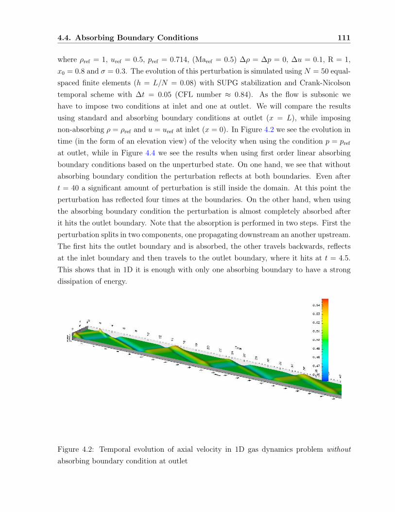
4.4. Absorbing Boundary Conditions 111
where ρref = 1, uref = 0.5, pref = 0.714, (Maref = 0.5) ∆ρ = ∆p = 0, ∆u = 0.1, R = 1,
x0 = 0.8 and σ = 0.3. The evolution of this perturbation is simulated using N = 50 equal-
spaced finite elements (h = L/N = 0.08) with SUPG stabilization and Crank-Nicolson
temporal scheme with ∆t = 0.05 (CFL number ≈ 0.84). As the flow is subsonic we
have to impose two conditions at inlet and one at outlet. We will compare the results
using standard and absorbing boundary conditions at outlet (x = L), while imposing
non-absorbing ρ = ρref and u = uref at inlet (x = 0). In Figure 4.2 we see the evolution in
time (in the form of an elevation view) of the velocity when using the condition p = pref
at outlet, while in Figure 4.4 we see the results when using first order linear absorbing
boundary conditions based on the unperturbed state. On one hand, we see that without
absorbing boundary condition the perturbation reflects at both boundaries. Even after
t = 40 a significant amount of perturbation is still inside the domain. At this point the
perturbation has reflected four times at the boundaries. On the other hand, when using
the absorbing boundary condition the perturbation is almost completely absorbed after
it hits the outlet boundary. Note that the absorption is performed in two steps. First the
perturbation splits in two components, one propagating downstream an another upstream.
The first hits the outlet boundary and is absorbed, the other travels backwards, reflects
at the inlet boundary and then travels to the outlet boundary, where it hits at t = 4.5.
This shows that in 1D it is enough with only one absorbing boundary to have a strong
dissipation of energy.
Figure 4.2: Temporal evolution of axial velocity in 1D gas dynamics problem without
absorbing boundary condition at outlet

112 Chapter 4. Dynamic Boundary Conditions in CFD
Figure 4.3: Temporal evolution of axial velocity in 1D gas dynamics problem with ab-
sorbing boundary condition at outlet
4.4.3 Multidimensional Problems
For multidimensional problems we can make a simplified 1D analysis in the normal direc-
tion to the local boundary and with the flux Jacobian A in equation (4.12) replaced with
its projection onto the exterior normal n, as follows
Π−n (U− U) = 0,
Π−n = Sn Π−
V n S−1n ,
(Π−V n)jk =
1; if j = k and λj < 0,
0; otherwise.
C−1An = SnΛnS−1n , (Λn diagonal),
An = Alnl.
(4.22)
These conditions are perfectly absorbing for perturbations reaching the boundary normal
to the surface. For perturbations not impinging normally, the condition is partially ab-

4.4. Absorbing Boundary Conditions 113
||∆
U||
time
1e−14
1e−12
1e−10
1e−08
1e−06
0.0001
0.01
1
0 5 10 15 20 25 30 35 40 45 50
not absorbing
absorbing
Figure 4.4: Rate of converge of 1D gas dynamics problem with and without absorbing
boundary conditions
1e−16
1e−14
1e−12
1e−10
1e−08
1e−06
0.0001
0.01
1
0 100 200 300 400 500 600 700 800 900 1000
absorbing linear
absorbing non−linear
p=cnst (non absorbing)
||∆
U||
time step
Figure 4.5: Rate of converge of 1D gas dynamics problem in full non-linear regime with
different kind of absorbing boundary conditions

114 Chapter 4. Dynamic Boundary Conditions in CFD
sorbing, with a reflection coefficient that increases from 0 at normal incidence to 1 for
tangential incidence.
4.4.4 Absorbing Boundary Conditions for Nonlinear Problems
If the problem is non-linear, as the gas dynamics or shallow water equations, then the
flux Jacobian A is a function of the state of the fluid, and then the same happens for the
projection matrices Π±. If we can assume that the flow is composed of small perturbations
around a reference state Uref , then we can compute the projection matrix at the state
Uref
Π(Uref)−n (U−Uref) = 0. (4.23)
However, as long as the fluid state departs from the reference value the condition becomes
less and less absorbing.
Numerical Example. Varying Section Compressible 1D Flow
Consider a one-dimensional flow in a tube with a contraction of 2:1. The inlet Mach
number is 0.2 and the variation of area along the tube axis is
A(x) = A0
(1− C
tanh(x− Lx/2)
Lc
), (4.24)
where A0 is some (irrelevant) reference area, C is a constant given by C = (α−1)/(α+1),
α = Ain/Aout is the area ratio and Lc = 0.136 is a parameter controlling the width of
the transition. We impose ρ and u at the inlet and consider different outlet conditions,
namely
• non-absorbing, p =cnst,
• absorbing linear (see (4.19)), and
• absorbing non-linear (see (4.23)).
In Figure 4.4 and 4.5 we see the evolution in time of the state vector increment (‖∆U‖)for different absorbing and non-absorbing boundary conditions.
4.4.5 Riemann Based Absorbing Boundary Conditions
Suppose that we take for a small interval t ≤ t′ ≤ t + ∆t the state U(t) as the reference
state, then, during this interval we can take Π−(U(t)) as the projection operator onto
the incoming characteristics and the absorbing boundary conditions are

4.4. Absorbing Boundary Conditions 115
Figure 4.6: Georg Friedrich Bernhard Riemann (1826–1866)
Π−(U(t)) (U(t′)−U(t)) = 0. (4.25)
But regarding the equivalent expression (4.18) we can see that it can be written as
lj(U) · dU = 0, if λj < 0, (4.26)
where lj is the j-th left eigenvalue of the normal flux Jacobian. Note that, as lj is a
function of U, this is a differential form on the variable U. If it happens that this is a
exact differential, i.e.,
µ(U) lj(U) · dU = dwj(U), (4.27)
for some non-linear function wj and an ‘integration factor’ µ(U), then we could impose
wj(U) = wj(Uref), (for wj an incoming char.) (4.28)
which would be an absorbing boundary condition for the whole non-linear regime. The
functions wj are often referred as ‘Riemann invariants’ (RI) for the flux function.
For the 2D shallow water equations the Riemann invariants are well known (see Ref-
erence [San01]). For 1D channel flow, Riemann invariants are known for a few channel
shapes (rectangular and triangular). For general channel sections they are not known and
in addition there is not a general numerical method for computing them. They could
be computed by numerical integration of (4.27) along a path in state space, but the
integration factor is not known.
Riemann invariants are known for the shallow water equations
w± = u · n± 2√gh, (4.29)

116 Chapter 4. Dynamic Boundary Conditions in CFD
and for channel flow they are known only for rectangular and triangular channel shapes.
For the triangular case RI are
w± = u · n± 4√gh. (4.30)
For the gas dynamics equations, the well known Riemann invariants are invariant only
under isentropic conditions, so that they are not truly invariant. They are
w± = u± 2c
γ − 1. (4.31)
4.4.6 Absorbing Boundary Conditions Based on Last State
While integrating the discrete equations in time, we can take the state of the fluid in the
previous state as the reference state
Π−(Un) (Un+1 −Un) = 0. (4.32)
It is clear that the assumption of linearization is well justified, since in the limit of ∆t→ 0
we should have Un+1 ≈ Un. In fact, (4.32) is equivalent, for ∆t → 0 to (4.26), so that
if Riemann invariants exist, then this scheme preserves them in the limit ∆t → 0 and
∆x→ 0. We call this strategy ULSAR (for Use Last State As Reference).
However, if this scheme is used in the whole boundary, then the flow in the domain is
only determined by the initial condition, and it can drift in time due to numerical errors.
Also if we look for a steady state at a certain regime, one has no way to guarantee that
that regime will be obtained. For instance, if we want to obtain the steady flow around an
aerodynamic profile at a certain Mach number, then we can set the initial state with a non
perturbed constant flow at those conditions, but we cannot assure that the final steady
flow will preserve that Mach number. In practice we often use a mix of the strategies, with
linear boundary conditions imposed at inlet regions and absorbing boundary conditions
based on last state on the outlet regions.
Numerical Example. ULSAR Strategy Keeps RI Constant
Consider a 1D compressible flow example, as in §4.4.2, with ρref = 1, uref = 0.2, pref =
0.714, (Maref = 0.2), ∆ρ = ∆p = 0, ∆u = 0.6, R = 1, x0 = 0.5L = 2 and σ = 0.3. Note
that this represents a perturbation in velocity that goes from Ma =0.2 to 0.8, so that full
non-linear effects are evidenced. The evolution of this perturbation is simulated using
N = 200 equal-spaced finite elements (h = L/N = 0.08) with SUPG stabilization and
Crank-Nicolson temporal scheme with ∆t = 0.02 (CFL number ≈ 1.2). All values are

4.4. Absorbing Boundary Conditions 117
made nondimensional by selecting L, ρref and uref as reference values for length, density
and velocity. Absorbing boundary conditions based on the ULSAR strategy are applied at
both ends x = 0, L. The values of the Riemann invariants (4.31) are computed there and
they are plotted in Figure 4.7. It can be seen that the incoming RI (the right going w+) is
kept approximately constant at the left boundary x = 0 and the same happens, mutatis
mutandis, at the other boundary x = L. Convergence history is shown in Figure 4.8.
Note that absorption is very good, despite the full non-linear character of the flow.
w−
w+
time
x=0
x=L
left
−goi
ng R
I
x=0 time
righ
t−go
ing
RI
x=L
0 2 4 6 8 10 12 14 16
−4.8
−4.7
−4.6
−4.5
−4.4
−4.3
0 2 4 6 8 10 12 14 16
5.1
5.2
5.3
5.4
5.5
5.6
5.7
5.8
Figure 4.7: Riemann invariants at boundaries with ULSAR ABC’s
4.4.7 Imposing Nonlinear Absorbing Boundary Conditions
In this section we discuss how the absorbing boundary conditions can be integrated in a
numerical code. For linear systems, the discrete version of equation (4.11) is of the form
CUn+1
0 −Un0
∆t+ A
Un+11 −Un
0
h= 0,
CUn+1
k −Unk
∆t+ A
Un+1k+1 −Un
k−1
2h= 0, k ≥ 1
(4.33)

118 Chapter 4. Dynamic Boundary Conditions in CFD
||∆U
||
time[sec] 0.0001
0.001
0.01
0.1
1
0 1 2 3 4 5 6 7 8 9 10
Figure 4.8: Convergence history when using with ULSAR ABC’s
where Unk is the state at grid point k at time tn = n∆t. We assume a constant mesh step
size of h, i.e., xk = kh, and assume a boundary at mesh node x0 = 0. We have made a lot
of simplifications here, no source or upwind terms, and a simple discretization based on
centered finite differences was used. Alternatively, it can be thought as a pure Galerkin
FEM discretization with mass lumping. If the projector onto incoming waves Π+U has
Figure 4.9: Boris Grigorievich Galerkin (1871–1945)
rank n+ = n, then Π+U = I and the absorbing boundary condition reduce to U = Uref
(being Uref a given value or Un0 for ULSAR). This happens for instance in a supersonic
inlet for gas dynamics or an inlet boundary for linear advection. In this case we simply
replace the balance equation for the boundary node (the first equation in (4.33)) with the
absorbing condition U = Uref , keeping the balance between equations and unknowns.

4.4. Absorbing Boundary Conditions 119
Conversely, if the projector onto incoming waves Π+U has rank n+ = 0, then Π+
U = 0
and the absorbing boundary condition reduce to not imposing anything. This happens
for instance in a supersonic outlet for gas dynamics or an outlet boundary for linear
advection. In this case we simply discard the absorbing condition U = Uref . Again the
number of equations and unknowns is maintained.
The case is more complicated when 0 < n+ < n. We cannot simply add the absorbing
condition (either (4.19), (4.28) or (4.32)), because we can neither discard the boundary
balance equation nor keep it.
There are at least two strategies for imposing this non-linear boundary condition.
One is to replace the boundary balance equation for the outgoing waves with a null
first derivative condition. Then a discrete version can be generated with finite difference
approximations. (This requires, however, a structured mesh at least near the boundary).
The other is to resort to the use of Lagrange multipliers or penalization techniques. One
advantage of using Lagrange multipliers or penalization is that not only the boundary
conditions coefficients can easily be changed for non-linear problems, but also the number
of imposed boundary conditions. This is important for problems where the number of
incoming characteristics can not be easily determined a priori, or for problems where the
flow regime is changing from subsonic to supersonic, or the flow reverts. In the rest of
this section we will describe in detail this second strategy.
In the base of the characteristic variables V, (4.33) can be written as
Vn+10 −Vn
0
∆t+ Λ
Vn+11 −Vn
0
h= 0,
Vn+1k −Vn
k
∆t+ Λ
Vn+1k+1 −Vn
k−1
2h= 0, k ≥ 1.
(4.34)
For the linear absorbing boundary conditions (4.19) we should impose
Π+V (Vref) (V0 −Vref) = 0, (4.35)
while discarding the equations corresponding to the incoming waves in the first rows
of (4.34). Here Uref/Vref is the state about which we make the linearization.
Using Lagrange Multipliers
This can be done, via Lagrange multipliers in the following way
Π+V (Vref) (V0 −Vref) + Π−
V (Vref)Vlm = 0,
Vn+10 −Vn
0
∆t+ Λ
Vn+11 −Vn
0
h+ Π+
V (Vref)Vlm = 0,
Vn+1k −Vn
k
∆t+ Λ
Vn+1k+1 −Vn
k−1
2h= 0, k ≥ 1,
(4.36)

120 Chapter 4. Dynamic Boundary Conditions in CFD
where Vlm are the Lagrange multipliers for the imposition of the new conditions. Note
that, if j is an incoming wave (λj ≥ 0), then the equation is of the form
vj0 − vref0 = 0,
vn+1j0 − vn
j0
∆t+ λj
vn+1j1 − vn
j0
h+ vj,lm = 0,
vn+1jk − vn
jk
∆t+ λj
vn+1j,k+1 − vn
jk
2h= 0, k ≥ 1.
(4.37)
Note that, due to the vj,lm Lagrange multiplier, we can solve for the vjk values from the
first and last rows, while the value of the multiplier vj,lm ‘adjusts’ itself in order to satisfy
the equations in the second row.
On the other hand, for the outgoing waves (λj < 0), we have
vj,lm = 0,
vn+1j0 − vn
j0
∆t+ λj
vn+1j1 − vn
j0
h= 0,
vn+1jk − vn
jk
∆t+ λj
vn+1j,k+1 − vn
jk
2h= 0, k ≥ 1.
(4.38)
So that the solution coincides with the unmodified original FEM equation, and the La-
grange multiplier is vj,lm = 0.
Coming back to the U basis, we have
Π+U(Uref) (U0 −Uref) + Π−
U(Uref)Ulm = 0,
CUn+1
0 −Un0
∆t+ A
Un+11 −Un
0
h+ CΠ+
U(Uref)Ulm = 0,
CUn+1
k −Unk
∆t+ A
Un+1k+1 −Un
k−1
2h= 0, k ≥ 1.
(4.39)
Using Penalization
The corresponding formulas for penalization can be obtained by adding a diagonal term
scaled by a small regularization parameter ε to the first equation in (4.39)
−εUlm + Π+U (U0 −Uref) + Π−
U Ulm = 0,
CUn+1
0 −Un0
∆t+ A
Un+11 −Un
0
h+ Π+
U Ulm = 0;(4.40)
where, for the moment, we dropped the dependence of the projectors on Uref . Eliminating
Ulm from the first and second rows we obtain
CUn+1
0 −Un0
∆t+ A
Un+11 −Un
0
h+ Π+
U (Π−U + εI)−1 Π+
U(U0 −Uref) = 0. (4.41)
4.5. Dynamically Varying Boundary Conditions 121
Now, using projection algebra we can show that
(Π−U + εI)−1 = (
1
εΠ+
U +1
1 + εΠ−
U) (4.42)
so that the last term in (4.41) reduces to Π+U(U0 −Uref) and the whole equation is
CUn+1
0 −Un0
∆t+ A
Un+11 −Un
0
h+
1
εCΠ+
U(U0 −Uref) = 0. (4.43)
Here 1/ε can be thought as a large penalization factor.
4.4.8 Numerical Example. Viscous Compressible Subsonic Flow
Over a Parabolic Bump
In order to evaluate the absorption of waves impinging at fictitious boundaries, a 2D
test consisting of a compressible subsonic flow over a parabolic bump at Maref = 0.5 is
considered (see Figure 4.10). The idea is to assess how the length from bump trailing
edge to the fictitous outflow (Lout) affects the predicted forces and their time evolution.
Two set of simulation were carried out. One set considering non-absorbent boundary
conditions where variables are imposed as specified in Figure 4.10. At inlet wall the
imposed conditions are ρ = ρref = 1, u = uref = Maref
√γpref/ρref = 0.5 and v = 0. At the
outflow boundary pressure is imposed, i.e., p = pref = 1/γ, where γ = 1.4. The second set
of simulations is considering ULSAR non-reflecting conditions at channel inlet and outlet.
Initial state for both set of problems is U = (ρref , uref , 0, pref). Parameters in Figure 4.10
are: Lin = 1.4, Lbump = 2, hbump = 0.1 and Lout = 1, 2, 4, 8. The values are made
nondimensional by selecting L, ρref and uref as reference values for length, density and
velocity Figures 4.11 and 4.12 show how ULSAR conditions produce the wave absorption
at fictitious boundaries.
4.5 Dynamically Varying Boundary Conditions
4.5.1 Varying Boundary Conditions in External Aerodynamics
During a flow computation the number of incoming characteristics n+ may change. This
can occur due to a flow regime changing (i.e., from subsonic to supersonic) or due to a flow
sense changing (flow reversal). A typical case is the external flow around an aerodynamic
body as shown in Figure 4.13. Consider first a steady subsonic flow. The flow is normally
subsonic at the whole infinite boundary, even if some supersonic pockets can develop at
transonic speeds. Then the only two possible regimes are subsonic inlet (n+ = nd + 1, nd

122 Chapter 4. Dynamic Boundary Conditions in CFD
L in
Lbump
hbump
L out
ρuv
p
slip condition
slip condition
Figure 4.10: Problem geometry
Lout=1,no abso
Lout=2,no absoLout=4,no abso
Lout=1, abso
Lout=2,4,8, abso
Lout=8,no abso
−1.46
−1.44
−1.42
−1.4
−1.38
−1.36
−1.34
−1.32
−1.3
0 200 400 600 800 1000 1200
Fy [N
]
t [secs]
−1.46
−1.44
−1.42
−1.4
−1.38
−1.36
−1.34
−1.32
−1.3
0 200 400 600 800 1000 1200
Fy [N
]
t [secs]
Figure 4.11: y-Force
is the spatial dimension) and subsonic outlet (n+ = 1). We can determine whether the
boundary is inlet or outlet by looking at the projection of the unperturbed flow velocity
u∞ with the local normal n. For the steady supersonic case the situation is very different.
A bow shock develops in front of the body and forms a subsonic region which propagates
downstream. Far downstream the envelope of the subsonic region approaches a cone with
an aperture angle equal to the Mach angle for the undisturbed flow. At the boundary we
have now a supersonic inlet region, and on the outlet region we have both subsonic and
supersonic parts. The point where the flow at outlet changes from subsonic to supersonic
may be estimated from the Mach angle, but it may be very inaccurate if the boundary is
close to the body. Having a boundary condition that can automatically adapt itself to the

4.5. Dynamically Varying Boundary Conditions 123
Lout=1, abso
Lout=2,4,8, abso
t[secs]
Fy[N
]
−1.46
−1.44
−1.42
−1.4
−1.38
−1.36
−1.34
−1.32
0 10 20 30 40 50 60 70 80
Figure 4.12: y-Force evolution for absorbent conditions
whole possibilities can be of great help in such a case. Now, consider the unsteady case,
for instance a body slowly accelerated from subsonic to supersonic speeds. The inlet part
will change at some point from subsonic to supersonic. At outlet, some parts will change
also from subsonic to supersonic, and the separation between both parts will change its
position, following approximately the instantaneous Mach angle.
subsonic flow (Minf<1)
subsonic incomingrho,u,v
psubsonic outgoing
supersonic flow (Minf>1)
rho,u,v,p
M>1M<1
bow shock
p
supersonic outgoing
subsonic outgoing
(no field imposed)
Figure 4.13: Number of incoming/outgoing characteristics changing on an accelerating
body

124 Chapter 4. Dynamic Boundary Conditions in CFD
4.5.2 Aerodynamics of Falling Objects
An interesting case is the aerodynamics of a falling body[FKMN97, Bel99, Hua00, Hua01,
Hua02]. Consider, for simplicity, a two dimensional case of an homogeneous ellipse in free
fall. As the body accelerates, the pitching moments tend to increase the angle of attack
until it stalls (A). Then, the body starts to fall towards its other end, and accelerates while
its main axis aligns with gravity (B). As the body accelerates the pitching moment grows
until it eventually stalls again (C). The pattern is repeated during the downfall. This kind
of falling mechanism is typical of slender bodies with relatively small moment of inertia
like a sheet of paper and is called ‘flutter’. However, depending on several parameters,
but mainly depending on the moment of inertia of the body, if it has a large angular
moment at (B), it may happen that it rolls on itself, keeping always the same sense of
rotation. This kind of falling mechanism is called ‘tumble’ and is a tipical pattern for
thicker and massive objects. For massive objects (like a ballistic projectile, for instance)
tumbling may convert a large amount of potential energy in the form of rotation, causing
the object to rotate at very large speeds. As the body falls it accelerates and can reach
A
B
C
B
D
flutter tumble
Figure 4.14: Falling ellipse
supersonic speeds. This depends on the density of the body relative to the surrounding

4.5. Dynamically Varying Boundary Conditions 125
atmosphere, its dimensions and shape. As the weight of the body goes with ∝ L3, being
L the characteristic length, while the drag force goes with ∝ L2, larger bodies tend to
reach larger limit speeds and eventually reach supersonic regime.
One can model a falling body in several ways. In order to avoid the use of deform-
ing meshes, a fixed mesh attached to the body can be used. Then one can choose to
perform the computation in a non-inertial frame moving with the body or to perform
the computation in an inertial frame using a moving but not deforming mesh. In the
first case ‘inertial forces’ (Coriolis, centrifugal) must be added, while in the second case
convective terms must take into account the mesh velocity as in the ‘Arbitrary Lagrangian
Eulerian (ALE)’ formulation. In this example we choose to use the first strategy. The
Figure 4.15: Gaspard-Gustave de Coriolis (1792–1843)
computation of the flow is linked to the dynamics of the falling object. The strategy is
a typically staggered fluid/solid interaction process [Ceb96, LYC+98, LC96]. Basically
we solve the fluid problem in a non-inertial frame with inertial terms computed with the
actual state of the body (linear acceleration a, angular rotation velocity ω and angular
rotation acceleration ω). Also boundary conditions in the non-inertial frame at infinity
must take into account the actual linear and angular velocity of the object. The fluid
solver updates the state of the fluid from tn to tn+1. Then, with the state of the fluid at
tn+1 the forces exerted by the fluid on the body are computed. With these forces, the
equations for the rigid motion of the body are solved (six dof’s, accounting for two linear
position and velocities, rotation angle and its derivative).
Coming back to the boundary conditions issue, added the fact that the body can
accelerate and decelerate, and going back and forth from subsonic to supersonic speeds,
we have now to take into account the angle from which the unperturbed flow impinges on

126 Chapter 4. Dynamic Boundary Conditions in CFD
the body varies with time. So, as the body can rotate arbitrarily, the flow can impinge
from any direction relative to the non-inertial frame fixed to the body.
Numerical Example. Ellipse Falling at Supersonic Speed
As an example consider the fall of an ellipse with the following physical data
• a = 1, b = 0.6 (major and minor semi-axes, eccentricity e =√
1− b2/a2 = 0.8),
• m = 1, (mass),
• w = 2.5, (weight of body),
• r = 1, (radius of inertia),
• c.m. = (−0.15, 0.0), (center of mass),
• ρa = 1, (atmosphere density),
• p = 1, (atmosphere pressure),
• γ = 1.4, (gas adiabatic index γ = Cp/Cv),
• Rext = 10, (Radius of the fictitious boundary),
• uini = [0, 0, 1.39, 0, 1.3, 0], (ellipse initial position and velocity [x, y, θ, u, v, θ]).
These values are made nondimensional by selecting a, ρa and c0 as reference values for
length, density and velocity, so that the nondimensional quantities are ρ′a = 1, p′ = 1/γ,
u′ = 0.5, and in the following the prime indicating nondimensional quantities is dropped.
A coarse estimation of the limit speed v can be obtained by balancing the vertical forces
on the body, i.e., the drag on the body (Faero), the weight and the hydrostatic flotation
Faero +W + Ffloat = CDρav2A− ρsgV + ρagV, (4.44)
where V = πab is the volume of the body (the area in 2D) and A = 2b the area of the
section facing the fluid (length in 2D). CD = 0.2 is an estimation for the drag coefficient
of the body and ρs = m/V, ρa the densities of solid and atmosphere respectively. For the
data above this estimation gives a limit speed of v = 2.8 approximately. The speed of
sound of the atmosphere is c =√γp/ρa = 1.18, so that it is expected that the body will
reach supersonic speeds. Of course, if the body does reach supersonic speed, then the
drag coefficient will be higher and probably the average speed will be lower than that one
estimated above.
The initial conditions are the ellipse starting at velocity (0,−1.39), and an angle of its
major axis of 80with respect with the vertical, the fluid is initially at rest. The computed
trajectory until t = 50 time units is shown in Figure 4.16. The computed trajectory is
shown in a reference system falling at velocity v = (−0.5, 0.5) (this is done in order to
reduce the horizontal and vertical span of the plot). In Figures 4.17 we see colormaps of

4.6. Conclusions 127
Mach number at six instants, in the non inertial frame fixed to the body. The instants
are marked as A,B,C and identified in the trajectory. Note that as the ellipse rotates,
each part of the boundary experiments all kind of regimes and the absorbing boundary
condition copes with all of them. Note also that the artificial boundary is located very
near to the body, the radius of the external circle is 3.25 times the major semi-axis of
the ellipse (in the case simulated with the minor external radius, i.e., Rext = 5). In
C
B
A
Figure 4.16: Computed trajectory of falling ellipse
Figure 4.18 the velocities of the ellipse are shown in order to evaluate the absorption of
ULSAR conditions when waves reach boundaries as the ellipse falls and tumble/flutter
when the fictitious boundary (exterior circle) is located at Rext = 5m and Rext = 10m
and the size of finite elements remain constant.
4.6 Conclusions
Absorbing boundary conditions reduce computational cost by allowing to put the artificial
exterior boundary closer to the region of interest. Extension to the non-linear cases can

128 Chapter 4. Dynamic Boundary Conditions in CFD
be done either by using Riemann invariants or by using the state at the previous time
step as reference state for a linearized boundary condition. In complex simulations the
number of incoming characteristic waves may vary during the computation or may not be
known a priori. In those cases absorbing boundary conditions can be imposed with the
help of Lagrange multipliers or penalization techniques.

Figure 4.17: Ellipse falling at supersonic speeds. Colormaps of |u|. Station A (t = 3.75),
station B (t = 6.25), station C (t = 10). Stations in the trajectory refer to Figure 4.16.
Results are shown in a non-inertial frame attached to the ellipse

u,Rext=5
u,Rext=10
v,Rext=10
v,Rext=5
t[secs]
u,v[
m/s
ec]
−3.5
−3
−2.5
−2
−1.5
−1
−0.5
0
0.5
1
0 5 10 15 20 25 30
Figure 4.18: Ellipse velocities for different external radius

Chapter 5
Strong Coupling Strategy for
Fluid-Structure Interaction
Problems in Supersonic Regime Via
Fixed Point Iteration
I am not sure that I exist,
actually.
I am all the writers that I have read,
all the people that I have met,
all the women that I have loved;
all the cities that I have visited,
all my ancestors...
Perhaps I would have liked to be my father,
who wrote and had the decency of not publishing.
Nothing, nothing, my friend;
what I have told you: I am not sure of anything,
I know nothing...
Can you imagine that I not even know the date of my death?
Jorge Luis Borges, Attributed
131

132Chapter 5. Strong Coupling Strategy for Fluid-Structure Interaction
Problems in Supersonic Regime Via Fixed Point Iteration
In this chapter some results on the stability of the time integration when solving
fluid/structure interaction problems with strong coupling via fixed point iteration strategy
are presented. The flow-induced vibration of a flat plate aligned with the flow direction
at supersonic Mach number is studied. The precision of different predictor schemes and
the influence of the partitioned strong coupling on stability are discussed.
5.1 Introduction
Multidisciplinary and multiphysics coupled problems represent nowadays a paradigm
when studying/analyzing even more complex phenomena that appear in nature and in new
technologies. There exists a great number of problems where different physical processes
(or models) converge, interacting in a strong or weak fashion (e.g., Acoustics/Noise distur-
bances in flexible structures, Magneto-Hydrodynamics devices, Micro-Electro-Mechanical
devices, Thermo-Mechanical problems like continuous casting process, Fluid/Structure in-
teraction like wing flutter problem or flow-induced pipe vibrations). In the fluid/structure
interaction area, the dynamic interaction between an elastic structure and a compress-
ible fluid has been the subject of intensive investigations in the last years (see Refer-
ences [GR05, PF01, Lef05]). This part of the present thesis concerns with the numerical
integration of this type of problems when they are coupled in a loose or strong manner.
For simple structural problems (like hinged rigid rods with one or two vibrational dof’s)
it is possible to combine into a single (simple) formulation the fluid and the structural
governing equations (see Reference [DCC+95]). In those cases, a fully explicit or fully
implicit treatment of the coupled fluid/structure equations is attainable. Nevertheless,
for complex/large scale structural problems, the simultaneous solution of the fluid and
structure equations using a ‘monolithic’ scheme may be mathematically unmanageable
or its implementation can be a laborious task. Furthermore, the monolithic coupled
formulation would change significantly if different fluid and/or structure models were
considered.
An efficient alternative is to solve each sub-problem in a partitioned procedure where
time and space discretization methods could be different. Such a scheme simplifies ex-
plicit/implicit integration and it is in favor of the use of different codes specialized on each
sub-area. In this application a staggered fluid/structure coupling algorithm is considered.
A detailed description of the ‘state of the art’ in the computational fluid/structure in-
teraction area can be found in works [PF01, FPF01, PF00, DP06] and the references
therein.
Beyond the physical and engineering importance, this problem is interesting from the

5.2. Strongly Coupled Partitioned Algorithm Via Fixed Point Iteration 133
computational point of view as a paradigm of multiphysics code implementation that
reuses preexistent fluid and elastic solvers. The partitioned algorithm is implemented in
the PETSc-FEM code (www.cimec.org.ar/petscfem) which is a parallel multi-physics
finite element program based on the Message Passing Interface MPI and the Portable
Extensible Toolkit for Scientific Computations PETSc. Two instances of the PETSc-FEM
code simulate each sub-problem and communicate interface forces and displacements via
Standard C FIFO files or ‘pipes’. The key point in the implementation of this partitioned
scheme is the data exchange and synchronization between both parallel processes. These
tasks are made in a small external C++ routine.
5.2 Strongly Coupled Partitioned Algorithm Via Fixed
Point Iteration
In this section the temporal algorithm that performs the coupling between the structure
and the fluid codes is described. It is a fixed point iteration algorithm over the states
of both fluid and structure systems. Each iteration of the loop is called a ‘stage’, so if
the ‘stage loop’ converges, then a ‘strongly coupled’ algorithm is obtained. Hereafter, this
algorithm is called ‘staged algorithm’. The basic staggered algorithm considered in this
section proceeds as follows: (i) transfer the motion of the wet boundary of the solid to
the fluid problem, (ii) update the position of the fluid boundary and the bulk fluid mesh
accordingly, (iii) advance the fluid system and compute new pressures (and the stress field
if compressible Navier-Stokes model is adopted), (iv) convert the new fluid pressure (and
stress field) into a structural load, and (v) advance the structural system under the flow
loads. Such a staggered procedure, which can be treated as a weakly coupled solution
algorithm, can also be equipped with an outer loop in order to assure the convergence of
the interaction process. The algorithm can be stated as follow
where
wn : is the fluid state (ρ,v, p) at time tn,
un : is the structure state (displacements) at time tn,
un : are structure velocities at time tn,
Xn : are fluid mesh node positions at time tn,
nstep : is the number of time steps in the simulation,
nstage : is the number of stages in the coupling scheme
nnwt : is the number of Newton loops in the non-linear problem,
CMD : is intended for Computational Mesh Dynamics,

134Chapter 5. Strong Coupling Strategy for Fluid-Structure Interaction
Problems in Supersonic Regime Via Fixed Point Iteration
Algorithm 2: Strong FSI coupling via fixed point iteration
1: Initialize variables:
2: for n = 0 to nstep do Main time step loop 3: tn = n∆t,
4: CFD CODE: 5: receive un from STRUCTURE
6: Xn = CMD(un) run CMD code 7: u(n+1)P = u(n+1,0) = predictor(un,un−1) compute predictor 8: STRUCTURE CODE: 9: receive wn from FLUID fluid state
10: for i = 0 to nstage do stage loop 11: CFD CODE: 12: receive u(n+1,i) from STRUCTURE
13: Xn+1,i+1 = CMD(un+1,i)
14: Compute skin normals and velocities 15: for k = 0 to nnwt do Fluid Newton loop 16: wn+1,i+1 = CFD(wn,Xn+1,i+1,Xn)
17: end for
18: send wn+1,i+1 to STRUCTURE
19: FLUID CODE: after each stage iteration 20: CSD CODE: 21: receive wn+1,i+1 from FLUID;
22: compute structural loads (wn,wn+1,i+1)
23: for k = 0 to nnwt do Structure Newton loop 24: un+1,i+1 = CSD(wn,wn+1,i+1)
25: end for
26: send un+1,i+1 to FLUID
27: STRUCTURE CODE: after each stage iteration 28: end for
29: FLUID CODE: after time each step 30: send un to FLUID;
31: STRUCTURE CODE: after each time step 32: send wn to STRUCTURE
33: end for

5.2. Strongly Coupled Partitioned Algorithm Via Fixed Point Iteration 135
CSD : for Computational Structure Dynamics,
CFD : for Computational Fluid Dynamics.
5.2.1 Notes on the Fluid/Structure Interaction (FSI) Algorithm
• Two codes (CFD and CSD) are running simultaneously. For simplicity, the basic
algorithm can be thought as if there were no ‘concurrence’ between the codes,
i.e., at a given time only one of them is running. This can be controlled using
‘semaphores’ and this is done using MPI ‘synchronization messages’.
• The most external loop is over the time steps. Internal to it is the ‘stage loop’.
‘Weak coupling’ is achieved if only one stage is performed (i.e., nstage = 1). In each
stage the fluid is first advanced using the previously computed structure state un
and the current estimate value un+1,i. In this way, a new estimate for the fluid state
wn+1,i+1 is computed. Next the structure is updated using the forces of the fluid
from states wn and wn+1,i+1. At the first stage, the state un+1,0 is predicted using
a second or higher order approximation (see equation (5.2)). Inside the stage loop
there are Newton loops for each code to solve the non-linearities. In this application
the Computational Structure Dynamics (CSD) is linear, so nnwt = 1.
• Once the coordinates of the structure are known, the coordinates of the fluid mesh
nodes are computed by a ‘Computational Mesh Dynamics’ code, which is symbolized
as
Xn = CMD(un). (5.1)
Even though the CMD may be performed with a general strategy using both nodal
reallocation or remeshing, in this chapter only the former is adopted, keeping the
topology unchanged. Relocation of mesh nodes can be done using an elastic or
pseudo-elastic model (see Reference [LNST06]) through a separate PETSc-FEM
parallel process (code named MESH-MOVE). For the simple geometry of the exam-
ple a simple spine strategy is used.
• The general form of the predictor for the structure state was taken from Refer-
ence [PF01] and can be written as
u(n+1)P = α0∆tun + α1∆t(u
n − un−1). (5.2)
It is at least first order accurate when no predictor is employed and it may be
improved to second order using the above predictor with some values for α0 and
α1 according to the problem at hand. To understand how to specify these two
parameters a simple two dof’s wake oscillator model represented by two second

136Chapter 5. Strong Coupling Strategy for Fluid-Structure Interaction
Problems in Supersonic Regime Via Fixed Point Iteration
order differential equations as follows
mz z + cz z + kzz = fz(y, y, y, t),
myy + cyy + kyy = fy(z, z, z, t),(5.3)
with (m, c, k) the mass, the damping and the stiffness parameters for each dof and
y, z representing the structure and the fluid simple model. The forcing terms at the
right hand side contain the coupling between the two blocks. This coupling may be
formulated in terms of the main variables and their two first derivatives, generally
velocities and accelerations. If the coupling contains only the main variables, i.e.,
fz(y, t) and fy(z, t), the predictor with α0 = 1 and α1 = 0 achieves second order
accuracy in time solutions. If the coupling contains velocities it is necessary to use
α1 = 1/2 to recover second order in time. In fluid structure interaction problems
solved via ALE it is known that the mesh velocity dependent of the fluid-solid
interface velocity is incorporated in the formulation, therefore to guarantee second
order accuracy in time it is necessary to use α0 = 1 and α1 = 1/2 for the predictor.
Note that, if the trapezoidal (Simpson’s) rule with α = 1/2 is used for both the
structure and the fluid and the predictor is chosen with at least second order preci-
sion, then the whole algorithm is second order, even if only one stage is performed.
• At the beginning of each fluid stage there is a computation of skin normals and
velocities. This is necessary due to the time dependent slip boundary condition for
the inviscid case implemented as a constraint (see equation (5.5)) or also in the case
of using a non-slip boundary condition for the viscous case where the fluid interface
has the velocity of the moving solid wall, i.e., v|Γg = v|Γg = u|Γg .
Figure 5.1: Thomas Simpson (1710–1761)

5.3. Description of Test Case 137
5.3 Description of Test Case
The flutter of a flat solid plate aligned with a gas flow at supersonic Mach numbers (see
Figure 5.2) is studied. A uniform fluid at state (ρ∞, U∞, p∞) flows over an horizontal rigid
wall y = 0 parallel to it. This test case has been studied also in [PF01]. In a certain
(ρ∞
, U∞
, p∞
)
x
y
A
C
B
D
u(x)
L
Figure 5.2: Description of test
region of the wall (0 ≤ x ≤ L) the wall deforms elastically following thin plate theory,
i.e.,
mu+D∂4u
∂x4= −(p− p∞) + f(x, t), (5.4)
where m is the mass of the plate per unit area in kg/m2, D = Et3/12(1− ν2) the bending
rigidity of the plate module in Nm, E is the Young modulus in Pa, t the plate thickness in
m, ν the Poisson modulus, u the normal deflection of the plate in m, defined on the region
0 ≤ x ≤ L and null outside this region, p the pressure exerted by the fluid on the plate in
Pa and f is an external force in N and will be described later. The plate is clamped at both
ends, i.e., u = (∂u/∂x) = 0 at x = 0, L. For the sake of simplicity the fluid occupying
the region y > 0 is inviscid. The compressible Euler model with SUPG stabilization
and ‘anisotropic shock-capturing’ method is considered (see Reference [TS04]). A slip
condition is assumed
(v − vstr) · n = 0 (5.5)
on the (curved) wall y = u(x), where
vstr = (0, u),
n ∝ (−∂u∂x, 1)
(5.6)

138Chapter 5. Strong Coupling Strategy for Fluid-Structure Interaction
Problems in Supersonic Regime Via Fixed Point Iteration
are the velocity of the plate and its unit normal. Finally, initial conditions for both the
fluid and the plate are taken as
u(x, t = 0) = u0(x),
u(x, t = 0) = u0(x),
(ρ,v, p)x,t=0 = (ρ,v, p)0, for y ≥ u0(x).
(5.7)
Note that for the fluid pressure load on the plate the free stream fluid pressure is
subtracted so that in the absence of any external perturbation (f ≡ 0) the undisturbed
flow (ρ,v, p)x,t ≡ (ρ,v, p)∞ is a solution of the problem for the initial conditions
u ≡ 0,
u ≡ 0,
(ρ,v, p)x,t=0 ≡ (ρ,v, p)∞.
(5.8)
5.3.1 Dimensionless Parameters
As the fluid is inviscid, it is determined by the ‘adiabatic index’ γ = Cp/Cv = 1.4 for air,
and the Mach number M∞ = U∞/c∞, where c∞ is the speed of sound c =√γp/ρ for the
undisturbed state.
Another dimensionless parameter can be built by taking the ratio between the char-
acteristic time of the structure Tstr =√mL4/D, and the characteristic time of the fluid
Tfl = L/U∞. Then, the dimensionless number NT is defined as the square of the ratio of
both characteristic times
NT =
(Tfl
Tstr
)2
=D
mL2U∞2 . (5.9)
Finally, a (dimensionless) number can be formed by taking the ratio between the mass of
the fluid being displaced by the structure and the structure mass
NM =ρ∞L
3
mL2=ρ∞L
m. (5.10)
The same parameters as reported in Reference [PF01] are considered. In this contribution,
flutter was studied near the point M∞ = 2.27, NT = 4.3438×10⁻⁵ and NM = 0.054667.
The flutter region was studied by varying the M∞ value while keeping ρ∞ and the structure
parameters (m, L, D) constant (so that NM is constant and NT ∝ M∞−2), and the same
approach is taken here. The dimensionless parameters are obtained by choosing the

5.3. Description of Test Case 139
following dimensional values
ρ∞ = 1 kg/m3,
p∞ = 1/γ = 0.71429 Pa,
U∞ = M∞, (since c∞ =√γp∞/ρ∞ = 1 m/sec),
D = 0.031611 Nm,
m = 36.585 kg/m2,
L = 2 m.
(5.11)
5.3.2 Houbolt’s Model
In this section the linear flutter instability by means of the modal analysis is studied.
First, the ‘Houbolt’s approximation’ (see Reference [Hou58]) is assumed for the fluid,
p− p∞ = Cx∂u
∂x+ Ct
∂u
∂t,
Cx =ρ∞U∞
2√M∞
2 − 1,
Ct =ρ∞U∞ (M∞
2 − 2)
(M∞2 − 1)3/2
.
(5.12)
With this approximation the governing equation for plate deflection (5.4) becomes
mu+D∂4u
∂x4= −Cx
∂u
∂x− Ct
∂u
∂t. (5.13)
Plane Wave Analysis
If an infinite plate is considered, a plane wave analysis may shed some light on the
mechanism that leads to a flutter behavior. Then, let us consider plane waves of the
form
u(x, t) = Reu ei(kx−ωt)
. (5.14)
Replacing (5.14) in (5.13) an implicit ‘dispersion law’ ω = ω(k) it is obtained
−ω2m+Dk4 = iCtω − ikCx. (5.15)
Regarding the last equation instability (flutter) occurs whenever Im ω > 0. Note that
lowering the mass ratio parameter NM while keeping NT and M∞ constant, it is equivalent
to scaling the fluid terms on the the right hand side of equation (5.12) by this factor. When
there is no fluid (NM → 0) the dispersion law simply reduces to
ω0 = ±√D
mk2. (5.16)

140Chapter 5. Strong Coupling Strategy for Fluid-Structure Interaction
Problems in Supersonic Regime Via Fixed Point Iteration
As expected, the eigenvalues are real, meaning neither damping nor amplification of the
waves. The positive (negative) sign corresponds to right-going (left-going) waves, i.e.,
waves that run in the same (opposed) direction as the fluid. The subscript 0 indicates
that this dispersion law is valid in the absence of fluid. Now assume that NM is small
enough so that the right hand side of equation (5.15) is a small perturbation to the terms
in the left hand side. Then a first order expansion of the left hand side with respect to ω
around ω0 can be done
−2mω0 δω = iCtω0 − ikCx, (5.17)
so that
ω ≈ ω0 − iCt
2m± i
Cx
2k√mD
. (5.18)
From this equation it is clear that the temporal term (the second one in the Houbolt
approximation (5.12)) has a stabilizing effect (negative imaginary part), while the spatial
term has a damping effect for left-going waves and destabilizing effect for right-going
ones, i.e., for those that run in the same direction as the fluid. Flutter occurs when the
destabilizing term is strong enough so as to overcome the stabilizing temporal term.
More physical insight is obtained analyzing the work that is done by the fluid onto the
plate. If a plane wave given by equation (5.14) is considered in its equivalent real form
u(x, t) = |u| cos(kx− ωt+ ϕ), (5.19)
with u = |u|eiϕ, then the instantaneous vertical velocity and pressure are
v =∂u
∂t= ω|u| sin(kx− ωt+ ϕ),
p− p∞ = (−Cxk + Ctω) |u| sin(kx− ωt+ ϕ).(5.20)
The instantaneous work done by the fluid onto the plate, averaged on a wave length
λ = 2π/k is
W = −∫ λ
0
pv dx,
= ω(Cxk − Ctω) |u|2λ2.
(5.21)
A positive work means that the structure is absorbing energy from the fluid, and then
has a destabilizing effect, while the opposite means dissipation of the structural wave
energy into the fluid. It can be seen (again) from equation (5.21) that the temporal
term has always a stabilizing effect, while the spatial term has a destabilizing effect when
sign(ω) sign(k) > 0, i.e., for right-going waves (traveling in the same sense of the fluid).
Note that at the basis of the destabilizing effect is the fact that the spatial term in
the Houbolt approximation produces a pressure perturbation field that is non-symmetric

5.3. Description of Test Case 141
with respect to the crest of the waves, i.e., before the crest ((du/dx) > 0) p − pref > 0
whereas after the crest ((du/dx) < 0) p− pref < 0. In inviscid subsonic flow the pressure
perturbation field would be symmetric.
Galerkin Model for the Finite Length Plate
The plate normal displacement is expanded in a global basis using
u(x) =N∑
k=1
akψk(x),
ψk(x) =4x(L− x)
L2sin(kπx/L).
(5.22)
These basis functions satisfy the essential boundary conditions for the plate equation
u = (∂u/∂x) = 0 at x = 0, L. Replacing the Houbolt approximation in equation (5.4),
using Galerkin method and integrating by parts as needed, the following matrix equation
is obtained
Ma + Ka + Hxa + Hta = 0, (5.23)
where
Mjk =
∫ L
0
mψj(x)ψk(x) dx,
Kjk =
∫ L
0
Dψ′′j (x)ψ′′k(x) dx,
Hx,jk =
∫ L
0
Cx ψj(x)ψ′k(x) dx,
Ht,jk =
∫ L
0
Ct ψj(x)ψk(x) dx.
(5.24)
Solution of these system of ODE’s can be found by standard operational methods by
replacing a(t) by the ansatz
a(t) = aeλt (5.25)
leading to the eigenvalue equation(λ2M + λHt + K + Hx
)a = 0. (5.26)
Flutter is detected whenever some eigenvalue λ has a positive real part.
Numerical Solution Details
• The series (5.22) are truncated at a certain number of terms N . Usually N = 10 or
20.

142Chapter 5. Strong Coupling Strategy for Fluid-Structure Interaction
Problems in Supersonic Regime Via Fixed Point Iteration
• Matrix entries for M, K, Ht and Hx are computed by approximating derivatives
with second order finite differences and integrating with a second order rule.
• The quadratic eigenvalue problem of size N is solved by converting it to a linear
eigenvalue problem of size 2N (and then finding eigenvalues and eigenvectors).
Results
Using for instance the values described in (5.11) with N = 20 terms in the series and
5000 intervals for computing the matrix coefficients integrals, and varying Mach from
1.8 to 3 the results shown in Figure 5.3 are obtained. For M∞ < Mcr = 2.265, all the
eigenvalues have negative real part being stable. For M∞ > Mcr = 2.265 there are two
complex conjugate roots with positive real part. In Figure 5.3 the real and imaginary
part of the unstable mode are plotted. For M∞ < Mcr = 2.265 the eigenvalue with
the lower frequency was taken as a continuation of the flutter mode. It was checked
that for M∞ < Mcr = 2.265 the plate does positive power on the fluid whereas for
M∞ > Mcr = 2.265 the converse is true. The instantaneous power done by the plate on
the fluid is
P =
∫ L
x=0
pu dx. (5.27)
In Figures 5.4 to 5.6 the form of the plate deflection of the flutter mode for Mach 2.22,
real(lambda)
imag(lambda)
imag
(lam
bda)
real(lambda)
Mach
Mach_cr = 2.265flutterno flutter
1.6 1.8 2 2.2 2.4 2.6 2.8 3 0.3
0.32
0.34
0.36
0.38
0.4
0.42
−0.02
−0.01
0
0.01
0.02
0.03
0.04
0.05
0.06
0.07
0.08
Figure 5.3: Lowest frequency mode for test case
2.27 and 2.35 can be observed. For each Mach, plate deflection, fluid pressure on the plate
and power that is being given by the plate on the fluid (pu) are shown.

5.3. Description of Test Case 143
−1
−0.8
−0.6
−0.4
−0.2
0
0.2
0.4
0.6
0.8
1
0 0.2 0.4 0.6 0.8 1 1.2 1.4 1.6 1.8 2
Figure 5.4: Mach 2.2, phase 0. Black= plate deflection, blue=pressure, green=power.
Quantities normalized (not to scale)
−1
−0.8
−0.6
−0.4
−0.2
0
0.2
0.4
0.6
0.8
1
0 0.2 0.4 0.6 0.8 1 1.2 1.4 1.6 1.8 2
Figure 5.5: Mach 2.27, phase 0
Flutter Region
A large number of flutter computations in the space NM , NT ,M∞ were performed in
order to determine the flutter region. A grid of 20 × 20 points in the region [0.001 ≤
−1
−0.8
−0.6
−0.4
−0.2
0
0.2
0.4
0.6
0.8
1
0 0.2 0.4 0.6 0.8 1 1.2 1.4 1.6 1.8 2
Figure 5.6: Mach 2.35, phase 0

144Chapter 5. Strong Coupling Strategy for Fluid-Structure Interaction
Problems in Supersonic Regime Via Fixed Point Iteration
NM ≤ 0.1]× [10−5 ≤ NT M∞2 ≤ 10−3] was scanned. For each point in the grid instability
is scanned in the Mach region 1.8 ≤ M∞ ≤ 3. The flutter region has the following
characteristics:NM
NT M∞2 < 200 no flutter for any Mach number,
NM
NT M∞2 > 300 flutter for the lowest Mach number considered (M∞ ≥ 1.8).
(5.28)
In the intermediate region flutter is produced. This suggests that flutter is highly corre-
lated to quantityNM
NtM∞2 =
ρ∞L3c∞D
, (5.29)
which happens to be independent of the density of the plate.
A simple model presented in Reference [DCC+95] draws a similar conclusion. The
explanation is as follows. In that reference, the term proportional to (∂u/∂t) is neglected.
This is true if the characteristic times of the structure are much lower than those of
the fluid, i.e., NT 1. This is a valid assumption because of all points in the grid
located in the region NT < 10−3 are considered. But if the temporal term in the Houbolt
approximation is neglected the characteristic equation can be written in the form
det(λ2M + K + Hx) = 0, (5.30)
whereλ =
√mλ,
M =1√m
M.(5.31)
As now the coefficients in M, K, Hx do not depend on m, neither do the eigenvalues of
equation (5.30), and then by (5.31) the λ eigenvalues are of the form
λj =λj√m, (5.32)
with λ not depending on m. This means that the sign of the real part of the λ is
independent of m.
5.3.3 FSI Code Results
The aeroelastic problem defined above was modeled with the strongly coupled partitioned
algorithm described in section §5.2 with a mesh of 12800 quadrilateral elements for the
fluid and 5120 for the plate. As the flow is supersonic only a small entry section of 1/8L
upstream the plate and 1/3L downstream is considered. The vertical size of the com-
putational domain was chosen as 0.8L. It is assured that no reflection from the upper
boundary affects the plate itself when considering these sizes for the fluid domain.

5.3. Description of Test Case 145
Determination of Flutter Region
This section presents some results obtained with PETSc-FEM code using the weak cou-
pling between fluid and structure, i.e., nstage = 1. The physical characteristics of the
plate are the same as in previous section. In order to find (numerically) the critical Mach
number for this problem a sweep in the Mach number in the range of 1.8 to 3.2 was done.
Results for some Mach numbers can be seen in Figures 5.7 to 5.12. In these plots the time
evolution of displacements of several points distributed along the skin plate are shown.
The fluid density field and the structure displacement at Mach=3.2 (flutter region) for a
given time step is shown in Figures 5.13 and 5.14. For Mach numbers below the
-0.002
-0.0015
-0.001
-0.0005
0
0.0005
0.001
0.0015
0.002
0 0.5 1 1.5 2 2.5 3 3.5 4 4.5
plat
e de
flect
ion
in d
istri
bute
d po
ints
[m]
time [sec]
Figure 5.7: Plate deflection in distributed points along plate at M=1.8
Mcr, Figures 5.7 to 5.9, the maximum plate displacement grows until the forces exerted
by the fluid dump the plate displacements. The time needed to reduce the response a
given factor (30% for instance) grows with the Mach number. For Mach numbers near the
Mcr, Figure 5.10, the maximum amplitude grows slightly. The flutter mode is triggered
at this point. For Mach numbers above the Mcr, Figures 5.11, 5.12, 5.13 and 5.14, the
fluid forces cannot damp the structure response and displacements grow without limit in
a unstable fashion according to the theory.
Time Accuracy
If the stage loop converges, i.e., (u,w)n+1,i → (u,w)n+1,∗, then it can be shown that the
limit states (u,w)n+1,∗ satisfy the fully implicit, strong coupled equations. The main effect

146Chapter 5. Strong Coupling Strategy for Fluid-Structure Interaction
Problems in Supersonic Regime Via Fixed Point Iteration
-0.005
-0.004
-0.003
-0.002
-0.001
0
0.001
0.002
0.003
0.004
0.005
0 0.5 1 1.5 2 2.5 3 3.5 4
plat
e de
flect
ion
in d
istri
bute
d po
ints
[m]
time [sec]
Figure 5.8: Plate deflection in distributed points along plate at M=2.225
-0.005
-0.004
-0.003
-0.002
-0.001
0
0.001
0.002
0.003
0.004
0.005
0 0.5 1 1.5 2 2.5 3 3.5 4
plat
e de
flect
ion
in d
istri
bute
d po
ints
[m]
time [sec]
Figure 5.9: Plate deflection in distributed points along plate at M=2.25
of the staged algorithm is to have a strong coupling and then, enhanced stability, regardless
the time accuracy, i.e., second or higher order temporal schemes can be achieved with a
non-staged weak algorithm, while a strong coupled staged algorithm not necessarily have
high order accuracy. In Figure 5.15 the error obtained after the simulation of a certain
fixed amount of time t0 and increasing time refinement is shown. The exact solution is
estimated through a Richardson extrapolation with the two more refined simulations for
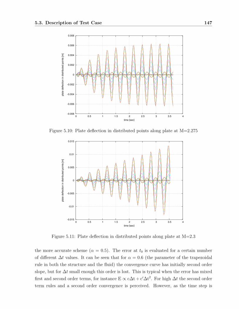
5.3. Description of Test Case 147
-0.008
-0.006
-0.004
-0.002
0
0.002
0.004
0.006
0.008
0 0.5 1 1.5 2 2.5 3 3.5 4
plat
e de
flect
ion
in d
istri
bute
d po
ints
[m]
time [sec]
Figure 5.10: Plate deflection in distributed points along plate at M=2.275
-0.015
-0.01
-0.005
0
0.005
0.01
0.015
0 0.5 1 1.5 2 2.5 3 3.5 4
plat
e de
flect
ion
in d
istri
bute
d po
ints
[m]
time [sec]
Figure 5.11: Plate deflection in distributed points along plate at M=2.3
the more accurate scheme (α = 0.5). The error at t0 is evaluated for a certain number
of different ∆t values. It can be seen that for α = 0.6 (the parameter of the trapezoidal
rule in both the structure and the fluid) the convergence curve has initially second order
slope, but for ∆t small enough this order is lost. This is typical when the error has mixed
first and second order terms, for instance E ∝ c∆t + c′∆t2. For high ∆t the second order
term rules and a second order convergence is perceived. However, as the time step is

148Chapter 5. Strong Coupling Strategy for Fluid-Structure Interaction
Problems in Supersonic Regime Via Fixed Point Iteration
-0.25
-0.2
-0.15
-0.1
-0.05
0
0.05
0.1
0.15
0.2
0 0.2 0.4 0.6 0.8 1 1.2 1.4 1.6
plat
e de
flect
ion
in d
istri
bute
d po
ints
[m]
time [sec]
Figure 5.12: Plate deflection in distributed points along plate at M=3.2
diminished, at a certain point the first term rules and the slope switches to first order.
For α = 0.5 the curve is O(∆t2) on the whole studied range of ∆t. When using α = 0.5
with no predictor (equation (5.2)), a second order convergence is still obtained, but the
convergence slightly slows down in the very last segment. Note that in this case the
scheme is second order, except for the fluid-structure interaction. As the interaction is
weak, perhaps the first order convergence can be observed for smaller time steps.
Convergence of Stage Loop
The convergence of the stage loops has been assessed by running the test case over 20
time steps and performing 10 stages at each time step. In Figure 5.16 the convergence of
the fluid state (i.e., ‖un+1,i+1 − un+1,i‖) for all the time steps (convergence curves of the
time steps are concatenated) is shown. Analogously, the convergence of the structure is
plotted in Figure 5.17. The average convergence is one order of magnitude per stage or
higher, suggesting that for such a situation a small nstage (2 or 3) would be enough.
Stability of the Staged Algorithm
The following numerical test allows to evaluate the stability of the staged algorithm
presented in section §5.2. The example is similar to the aeroelastic test case presented in
section §5.3 with some different parameters for the plate in order to produce larger plate
deformations and stronger instabilities. Some parameters are similar to those presented in

5.3. Description of Test Case 149
Figure 5.13: Fluid and structure fields at M=3.2
equation (5.11). Here, only the parameters that have been modified and the dimensionless
parameters that may be obtained with them are included.
U∞ = M∞ = 2
t = 0.06
ν = 0.33
m = 0.002
E = 39.6
D = 8.010−4
NT =D
mL2U∞2 = 0.025
NM =ρ∞L
m= 1000.0
(5.33)
Therefore according to the section §5.3.2
NM
NT M∞2 = 10000 > 300 (5.34)
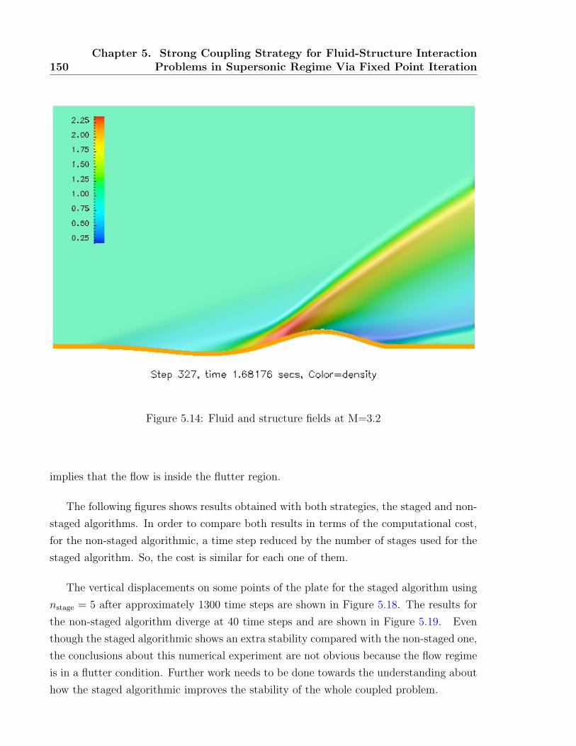
150Chapter 5. Strong Coupling Strategy for Fluid-Structure Interaction
Problems in Supersonic Regime Via Fixed Point Iteration
Figure 5.14: Fluid and structure fields at M=3.2
implies that the flow is inside the flutter region.
The following figures shows results obtained with both strategies, the staged and non-
staged algorithms. In order to compare both results in terms of the computational cost,
for the non-staged algorithmic, a time step reduced by the number of stages used for the
staged algorithm. So, the cost is similar for each one of them.
The vertical displacements on some points of the plate for the staged algorithm using
nstage = 5 after approximately 1300 time steps are shown in Figure 5.18. The results for
the non-staged algorithm diverge at 40 time steps and are shown in Figure 5.19. Even
though the staged algorithmic shows an extra stability compared with the non-staged one,
the conclusions about this numerical experiment are not obvious because the flow regime
is in a flutter condition. Further work needs to be done towards the understanding about
how the staged algorithmic improves the stability of the whole coupled problem.

5.4. Stability of the Weak/Strong Staged Coupling Outside the FlutterRegion 151
10−3 10−2 10−110−9
10−8
10−7
10−6
10−5
10−4
Dt
|| U
− U
est ||
Time accuracy for Fluid Structure Interaction problems
alpha=05 (final slope = 2)
alpha=05 − no predictor (final slope = 1.75)
alpha=06
prop. to Dt^2
prop. to Dt
Figure 5.15: Experimentally determined order of convergence with ∆t for the uncoupled
algorithm with fourth order predictor
5.4 Stability of the Weak/Strong Staged Coupling
Outside the Flutter Region
This section describes the stability properties of the weak coupling when the free stream
conditions and plate parameters are such that the oscillations due to flutter do not appear.
The flutter region can be characterized by the dimensionless number FL = NM/NTM2∞
(see the previous section). Therefore, in order to study the stability behavior of the
weak/strong algorithms (nstage = 1 and nstage > 1, respectively) intrinsic to the physical
coupling, the region FL 200 is studied and particularly FL = 12 is chosen. This
non-dimensional number does not depend on the plate density m then a sweep can be
done on this variable in a wide range avoiding triggering flutter. The idea is to find a
value for this variable in which the weak coupling algorithms becomes unstable while the
strong coupling and the uncoupled problems remain stable (i.e., fluid pressures are not
transferred to the structure). To accomplish convergence in the non-linear loop for the
fluid problem 2 Newton iterations (typically for this problem, 3-5 orders of magnitude are
lowered in the residual in 2 Newton loops) are adopted. The mesh is the same as in the
previous simulations and the Courant number is CFL = 0.5. The plate mass varies in

152Chapter 5. Strong Coupling Strategy for Fluid-Structure Interaction
Problems in Supersonic Regime Via Fixed Point Iteration
0 20 40 60 80 100 120 140 160 180 20010−16
10−14
10−12
10−10
10−8
10−6
10−4
10−2
one time step
one stage
Nstep * Nstage
|| D
elta
( U
) ||
Fluid convergence (20 steps , 10 stages each)
Figure 5.16: Convergence of fluid state in stage loop
the range m = 35 to m = 0.0001. It was found that the value of m where instabilities
appear relies in the neighbor of m = 0.65. Above this value the weakly coupling scheme is
stable, below this, the weakly coupling algorithm is unstable meanwhile each sub-problem
(fluid and structure) are stable when considering no coupling. Instabilities disappear when
the strong coupling scheme with nstage = 2 is considered. Moreover, even when a lower
value of m is used, i.e., m = 0.0135 and CFL = 1, only 2 stages are enough to achieve
convergence of the strong coupling algorithm. Obviously, at this point each detached
problem is still stable (see Figures 5.20 and 5.21). In the case of m = 0.0001 a smaller
CFL number is needed (e.g., CFL = 0.5) in order to have at least 15 time steps in one
period (recall that the plate frequency depends on the plate density). Even though the
convergence of the coupled problem is not affected when considering a very small plate
density and a strong partitioned scheme, it is necessary to refine the fluid mesh in the
normal direction to the plate in order to have a better definition of the problem in that
direction, i.e., a wave train is propagated in the fluid with the plate frequency (recall that
the plate frequency grows as the plate density decrease, ωstr = 2π/Tstr = [mL4/D]−1/2).
In the coupled simulation the interaction may produce the amplification of the pressures
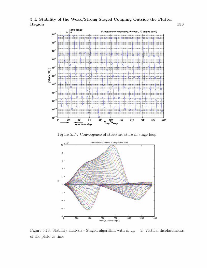
5.4. Stability of the Weak/Strong Staged Coupling Outside the FlutterRegion 153
0 20 40 60 80 100 120 140 160 180 20010−13
10−12
10−11
10−10
10−9
10−8
10−7
10−6
10−5
one time step
one stage
10−4
10−3
Nstep * Nstage
|| D
elta
( U
) ||
Structure convergence (20 steps , 10 stages each)
Figure 5.17: Convergence of structure state in stage loop
0 200 400 600 800 1000 1200 1400−8
−6
−4
−2
0
2
4
6
8
10x 10−3
Time [ # of time steps ]
uy
Vertical displacement of the plate vs time
Figure 5.18: Stability analysis - Staged algorithm with nstage = 5. Vertical displacements
of the plate vs time

154Chapter 5. Strong Coupling Strategy for Fluid-Structure Interaction
Problems in Supersonic Regime Via Fixed Point Iteration
0 5 10 15 20 25 30 35 40 45 50−12
−10
−8
−6
−4
−2
0
2
4x 10⁻⁴
Time [ # of time steps ]
uy
Vertical displacement of the plate vs time
Figure 5.19: Stability analysis - Non-staged algorithm. Vertical displacements of the plate
vs time
Figure 5.20: Unstable weak coupling for m = 0.0135 and CFL = 0.5
and plate displacements. This fact can be shown in Figures 5.22 and 5.23. Figure 5.22
shows the plate deflection when m = 0.00135 and mesh size of the fluid mesh near the
plate is hy = 0.018808 m and hx = 0.035625 m. Figure 5.23 shows the same results when

5.4. Stability of the Weak/Strong Staged Coupling Outside the FlutterRegion 155
Figure 5.21: Stable staged coupling for m = 0.0135, CFL = 1 and nstage = 2
considering an homogeneous refinement (i.e., hy = 0.00932 m and hx = 0.01781 m). The
coarse mesh exhibit a spurious vibration mode similar to a flutter mode that is corrected
in the finer mesh.
Figure 5.22: Strong partitioned scheme in a coarse mesh

156Chapter 5. Strong Coupling Strategy for Fluid-Structure Interaction
Problems in Supersonic Regime Via Fixed Point Iteration
Figure 5.23: Strong partitioned scheme in a fine mesh
5.5 Conclusions
Stability is enhanced through a strong coupling scheme and it shows to be necessary
for situations where the structural response is fast. Partitioned schemes using staged
strong coupling show to be very efficient avoiding the tedious and problem dependent
task of building a monolithic coupling formulation. For the benchmark considered in this
work two stages were enough for having the same behavior of the monolithic scheme.
Furthermore, the staged strategy provides a smooth blending between weak coupling and
strong coupling, i.e., moderately coupled problems that can not be treated with the pure
weak coupling approach, can be solved with the staged algorithm using few stages per
time step.
Time-accuracy is in agreement with the accuracy of the underlying fluid and structure
solvers, if an accurate enough predictor is used. Second order accuracy can be obtained
with second order fluid and structure solvers, and one stage coupling with a high order
predictor, as already reported in Reference [PF01].
The elastic flat plate problem is geometrically simple, but gives physical insight in the
flutter phenomena, and was very useful in testing the proposed algorithm in a wide range
of non-dimensional parameters.

Part III
Final Conclusions
157


Chapter 6
Overview and Final Remarks
The main goal of this thesis was the proposition, description and test of a new precondi-
tioner for Schur complement-based Domain Decomposition Methods that performs better
than classical ones in a wide range of flow problems and specially when advection terms
are high. The performance of the new preconditioner has been tested and compared with
other preconditioner/solvers that are extensively used in Computational Fluid Dynamics.
Details of the implementation and its testing were given.
Another goal of this thesis was the proposition of a set of local linear/non-linear dy-
namic boundary conditions for CFD application. It has been tested an absorbent bound-
ary conditions on fictitious boundaries where (energy) wave reflection is accomplished
when imposing conditions in a classical manner.
Also, in an ulterior part of this thesis have been treated fluid/structure interaction
problems in the supersonic regime of a compressible fluid that flows over/around elastic
bodies. In that section, a new partitioned algorithm for the time integration of coupled
governing equations has been proposed and tested. The proposed ‘staged’ algorithm can
be used to achieved either lose and strong coupling depending on the problem at hand.
During this thesis it has been published the following articles in referred journals
1. Rodrigo R. Paz and Mario A. Storti. ‘An Interface Strip Preconditioner for
Domain Decomposition Methods: Application to Hydrology’. International Journal
for Numerical Methods in Engineering, 62(13):1873-1894, 2005.
2. Rodrigo R. Paz, Norberto M. Nigro and Mario A. Storti. ‘On the ef-
ficiency and quality of numerical solutions in CFD problems using the Interface
Strip Preconditioner for domain decomposition methods’. International Journal for
Numerical Methods in Fluids, 52(1):89-118, (2006).
3. Storti, M. ; Dalcın, L. ; Paz, R. ; Yommi, A. ; Sonzogni, V. ; Nigro, N. ‘A
159

160 Chapter 6. Overview and Final Remarks
Preconditioner for Schur Complement Matrix’. Advances in engineering Software,
(2006). In press.
4. Lisandro Dalcın, Rodrigo R. Paz and Mario A. Storti. ‘MPI for Python’.
Journal of Parallel and Distributed Computing, 65(9):1108-1115, 2005.
5. Storti, M. ; Dalcın, L. ; Paz, R. ; Yommi, A. ; Sonzogni, V. ; Nigro,
N. ‘Interface Strip Preconditioner for Domain Decomposition Methods’. Journal of
Computational Methods in Sciences and Engineering, (2003). In press.
6. Mario A. Storti, Norberto M. Nigro and Rodrigo R. Paz. ‘Strong coupling
strategy for fluid-structure interaction problems in supersonic regime via fixed point
iteration’. Journal of Sound and Vibration. Submitted.
7. Mario A. Storti, Norberto M. Nigro, Rodrigo R. Paz and Lisandro Dalcın.
‘Dynamics boundary conditions in CFD’. Journal of Computational Physics. Sub-
mitted.
8. S. A. Vera; M. Febbo; C. G. Mendez; R. R. Paz. ‘Vibrations of a plate
with an attached two degree of freedom system’. Journal of Sound and Vibration,
285(1-2):457-466, 2004.
Besides, several articles have been submitted and presented in international confer-
ences on numerical methods for computational mechanics.

Part IV
Appendix
161


Appendix A
Functional Spaces
A.1 Some Used Sobolev Spaces
Let us denote by L2(Ω) the space of functions that are square integrable over its support
Ω. Let the standard inner product be a norm for this space
(u, v) =
∫Ω
uv, with the norm ||v0|| = (u, v)1/2. (A.1)
Figure A.1: Sergei Lvovich Sobolev (1908–1989)
Assume that k is a non-negative integer, then the Sobolev space Hk(Ω) is defined
using multi-index notation
Hk(Ω) =
u ∈ L2(Ω)| ∂|α|u
∂xα11 ∂x
α22 ...∂x
αndnd
∈ L2(Ω) ∀ |α| ≤ k
. (A.2)
given a n-tuple α = (α1, α2, ..., αnd) ∈ Rnd and non-negative integer |α| = α1+α2+...+αnd
.
163

164 Chapter A. Functional Spaces
Then, Hk(Ω) consists of square integrable functions all of whose derivatives of order
up to k are also square integrable. Hk(Ω) is equipped with the norm
||u||k =
k∑s=0
∑|α|=s
∣∣∣∣∣∣∣∣ ∂|α|u
∂xα11 ∂x
α22 ...∂x
αndnd
∣∣∣∣∣∣∣∣20
1/2
. (A.3)
For k = 0 we note in fact that the Sobolev space H0(Ω) is L2(Ω). In the case of k = 1
the Sobolev space is defined by
H1(Ω) =
u ∈ L2(Ω)| ∂v
∂xi
∈ L2(Ω), i = 1, 2, ..., nd
. (A.4)
The inner product associated with this space is
(u, v)1 =
∫Ω
(uv +
nd∑i=1
∂u
∂xi
∂v
∂xi
)dΩ, (A.5)
and the induced norm is
(u, u)1 = ||u||1 =√
(u, u)1. (A.6)
Frequently, we use the subspace
H10(Ω) =
v ∈ H1(Ω)|v = 0 on Γ
, (A.7)
whose elements have square integrable first derivatives over Ω and vanish on its boundary
Γ. Its inner product and norm coincide with those of H1(Ω).
Remark A.1.1. Note that the Sobolev spaces L2(Ω),H1(Ω) and H10(Ω) are Hilbert spaces
with corresponding inner products. Recall that a Hilbert space is a linear space with an
inner product in which all Cauchy sequences are convergent sequences.
Remark A.1.2. H10(Ω) is usually defined as the closure of C∞
0 (Ω) (the set of all contin-
uous functions with continuous derivatives whose support is a bounded subset of Ω) with
respect to the norm of ||.||1. That is, H10(Ω) is the set of all functions u in H1(Ω) such
that u is the limit in H1(Ω) of a sequence us∞s=0 whose us are in C∞0 (Ω).
A.2 Extension to Vector-Valued Functions
The finite element formulation deals not only with scalar-valued functions (such as pres-
sure and temperature) but also with vector-valued functions (e.g., velocity fields). For
A.2. Extension to Vector-Valued Functions 165
Figure A.2: David Hilbert (1862–1943)
Figure A.3: Augustin Louis Cauchy (1789–1857)
vector-valued functions with m components, that is uuu,vvv : Ω → Rm is essentially the same
as for scalar functions.
Consider a domain Ω ⊂ Rnd , nd ≥ 1 and denote by HHHk(Ω) (or [Hk(Ω)]m) the space of
vector functions with m components
uuu = (u1, u2, ..., um), (A.8)
for which each component ui ∈ Hk(Ω), 1 ≤ i ≤ m. The space HHHk(Ω) is equipped with an
inner product inducing the norm
||uuu||k =
√√√√ m∑i=1
||ui||2k. (A.9)
For the particular case of functions belonging to LLL2(Ω) = HHH0(Ω) the inner product is

166 Chapter A. Functional Spaces
given by
(uuu,vvv) =
∫Ω
uuu · vvvdΩ, (A.10)
and there should be no ambiguity in using the same notation to represent the inner
product of both scalar and vector-valued functions.

Appendix B
Resumen extendido en castellano
Tecnicas de Descomposicion de Dominio yProgramacion Distribuida en Mecanica de
Fluidos Computacional
B.1 El Metodo de Descomposicion de Dominios en
Mecanica de Fluidos Computacional
La diversidad de escalas de tiempo y de espacio presentes en problemas relacionados con
la mecanica de fluidos y su interaccion con cuerpos solidos (e.g., problemas de hidrologıa
superficial y subterranea acoplados o no, flujo de aire alrededor de cuerpos o vehıculos,
etc.) requiere un alto grado de refinamiento en las mallas utilizadas en el metodo de
elementos finitos y, por lo tanto, demanda grandes recursos computacionales.
La solucion de problemas en ‘gran escala’ en mecanica computacional tiene un desafıo
particular y es el de utilizar eficientemente los recursos disponibles [LTV97, SP96]. Si no se
utilizan adecuadas tecnicas numericas para reducir, optimizar y/o simplificar el problema,
es menester contar con grandes recursos computacionales para tratar el problema. Por otro
lado, el auge de computadoras cada vez mas rapidas y con mayor capacidad de calculo
167

168 Chapter B. Resumen extendido en castellano
hace que los problemas que se quieren resolver sean cada vez mas grandes y complejos
(i.e., mayores y mas variadas escalas, acople de distintos campos, modelos que tengan
en cuenta otras variables y su evolucion e interaccion con las demas, etc.). Es ası, que
los modelos matematicos son cada vez mas complejos y sofisticados haciendo que las
simulaciones de los sistemas resultantes sean extensas y complicadas. La restriccion sobre
los recursos computacionales disponibles esta siempre presente y por eso la urgencia en
el desarrollo y verificacion de tecnicas de solucion capaces de explotar eficientemente el
potencial de las modernas computadoras y la posibilidad de obtener soluciones de buena
calidad en un tiempo aceptable de simulacion (tiempo de CPU). La presente tesis nace
en esta necesidad.
Durante varias decadas se han desarrollado y probado tecnicas concernientes a solu-
ciones de problemas lineales que son resultado de la aplicacion del metodo de elementos
finitos (MEF) a ecuaciones diferenciales en derivadas parciales (EDDP) que tratan de
describir un conjunto de eventos de la fısica (e.g., mecanica de cuerpos solidos, dinamica
estructural, dinamica de fluidos, etc.). Hasta no hace mucho tiempo, la solucion directa
de estos sistemas era preferida a la solucion iterativa debido a su mayor robustez y al
caracter predictivo de su comportamiento. Sin embargo, la gran cantidad de tecnicas ite-
rativas que han sido desarrolladas, conjuntamente con la necesidad de resolver sistemas
de ecuaciones cada vez mas grandes en diferentes arquitecturas, han dado como resultado
una inclinacion al uso de este tipo de tecnicas y al desarrollo de nuevas.
Esta tendencia se viene dando desde 1970 cuando dos importantes desarrollos mar-
caron un punto de inflexion en la solucion de grandes sistemas de ecuaciones. Uno fue
la explotacion de la ‘baja densidad’ (por sparsity, matrices ralas o matrices con tasa de
llenado baja) de los sistemas que resultan de la aplicacion del MEF (como ası tambien
del metodo de diferencias finitas, MDF) a las EDDP. El otro fue el desarrollo de meto-
dos tales como los de Krylov (o metodos tipo gradientes conjugados). Gradualmente los
metodos iterativos (precondicionamiento e iteracion en el espacio de Krylov) comenzaron
a aproximarse en calidad a las soluciones provistas por los metodos directos. Particular-
mente, mucho se ha escrito sobre el metodo de gradientes conjugados precondicionado
para sistemas lineales simetricos que resultan de operadores simetricos (e.g., elasticidad
lineal y no lineal, flujo potencial, etc.).
Hoy, los grandes sistemas de ecuaciones obtenidos de las EDDP no lineales mediante
el MEF para problemas transitorios en dos y tres dimensiones, donde pueden haber va-
rias incognitas por nodo, son resueltos con metodos iterativos en computadoras de alta
performance (arquitecturas paralelas o vectoriales) debido a que requieren mucha me-
nor comunicacion entre los procesadores que la necesaria en metodos directos donde la

B.2. Ecuaciones de Gobierno 169
solucion de cada una de las incognitas esta acoplada con las demas.
El metodo de subestructuracion (o metodo de descomposicion de dominios e iteracion
sobre la matriz complemento de Schur para dominios no solapados) conduce a sistemas
reducidos mejor condicionados para la solucion mediante metodos de iteracion en el espa-
cio de Krylov. El numero de condicion de estos problemas se ve disminuido en un factor
1/h (∝ 1/h vs ∝ 1/h2 para el sistema global, siendo h la dimension caracterıstica de la
malla) y el costo computacional por iteracion no se ve encarecido debido a que las matrices
correspondientes a los grados de libertad correspondientes a los sub-dominios ya han sido
factorizadas. La eficiencia de estos metodos puede ser mejorada mediante el uso de pre-
condicionadores [Man93, BPS86, Cro02]. Diferentes tecnicas de precondicionamiento han
sido propuestas y la reduccion del numero de condicion de las matrices ha sido demostra-
da en el marco de ecuaciones diferenciales lineales elıpticas (e.g., precondicionadores del
tipo wire basket, Neumann-Neumann y sus variantes para los problemas de elasticidad y
flujo de Stokes).
En este trabajo se buscara solucionar eficientemente los sistemas de ecuaciones pro-
venientes de la discretizacion mediante el MEF o MDF de ecuaciones diferenciales no
lineales en derivadas parciales que representan modelos numericos de problemas reales
(como los descriptos arriba) considerados un desafıo para los metodos computacionales
actuales, usando tecnicas de programacion avanzada que integran paradigmas de progra-
macion, i.e., programacion orientada a objetos y calculo distribuido (calculo en paralelo).
Es objetivo tambien el desarrollo de un codigo de elementos finitos orientado a objetos
(que reduce drasticamente las dependencias de implementacion entre subsistemas y que
conduce al principio de reusabilidad de disenos de interfases) que resuelva problemas de
la mecanica de fluidos computacional en gran escala en forma distribuida mediante la
tecnica de paso de mensajes (MPI/PETSc [GLS94, BGCMS04]). Esta tecnica es amplia-
mente explotable en arquitecturas de computadoras paralelas, tales como la de ‘clusters’
Beowulf [SSBS99].
B.2 Ecuaciones de Gobierno
Centralizaremos el trabajo en la solucion de las ecuaciones de Navier-Stokes para flui-
dos compresibles e incompresibles estabilizadas con el metodo SUPG/PSPG propuesto
por Tezduyar et al.[TMRS92]. Las ecuaciones de Navier-Stokes presentan dos dificulta-
des importantes en su solucion por el metodo de elementos finitos. La primera dificultad
es que a medida que el numero de Reynolds del flujo aumenta, el caracter advectivo
de estas es cada vez mayor (con los problemas que esto trae aparejado en cuanto a es-

170 Chapter B. Resumen extendido en castellano
tabilidad de la solucion [BH82]). Ademas, en el caso incompresible, esta condicion re-
presenta una restriccion para las ecuaciones mas que la evolucion de las cantidades en
juego. Debido a esto, solo algunas combinaciones de los espacios de interpolacion para
las velocidades y las presiones pueden ser utilizadas (i.e., debe satisfacerse la condicion
de Ladyzhenskaya-Brezzi-Babuska [Bre74], ver apendice §B.5). En el trabajo de Tezdu-
yar et al. el termino advectivo es estabilizado con el bien conocido metodo SUPG (por
Streamline Upwind Petrov/Galerkin). Un termino similar, llamado PSPG (por Pressure
Stabilizing Petrov/Galerkin) es introducido para estabilizar la presion. Una vez que las
ecuaciones son discretizadas, el sistema de ecuaciones diferenciales ordinarias resultante
son discretizadas en el tiempo mediante la regla trapezoidal.
Se abordara tambien la integracion temporal de las ecuaciones de Navier-Stokes con
esquemas de tipo desagregado como lo es el de Paso Fraccionado (por Fractional Step)
propuesto inicialmente por Chorin [Cho73] y Temam [Tem69]. A diferencia del esquema
monolıtico anteriormente senalado, los esquemas desagregados desacoplan el campo de
presiones del campo de velocidades solucionando por separado ambos problemas. Este
desacople permite para una dada potencia de calculo aumentar en gran medida el numero
de grados de libertad del problema (y por consiguiente refinar la malla o agrandar el
dominio de calculo si el problema lo requiriese). Un gran desventaja de este metodo es
que por razones de estabilidad (que seran contempladas en el contexto de esta tesis) el
paso de integracion esta acotado y es necesario un mayor tiempo de simulacion para
obtener soluciones estacionarias/periodicas.
B.2.1 Propiedades Continuas de los Fluidos
La idea de tratar a un medio fluido como un medio continuo es natural y ‘familiar’. Sin
embargo es necesario rever la hipotesis del continuo para evitar confusion cuando se habla
de ‘partıculas de fluido’ y ‘elementos materiales infinitesimales’. Las longitudes de escala y
tiempo del movimiento molecular son extremadamente pequenas en relacion a las escalas
que el hombre maneja habitualmente. Si consideramos al aire en condiciones normales
atmosfericas por ejemplo, el espacio medio entre moleculas es 3 · 10−9 m, el camino medio
entre partıculas, λp, es 6 · 10−8 m y el tiempo medio entre sucesivas colisiones de una
molecula es 10−10 s. En comparacion, la menor escala geometrica ` que se pueda considerar
en el flujo de un fluido es a menudo menor que 0,1 mm = 10−4 m, que para velocidades de
hasta 100 m/s supone una escala de tiempo mayor a 10−6 s. Por lo tanto, inclusive para
este ejemplo donde las escalas de tiempo y longitud del flujo son pequenas, estas exceden
las escalas moleculares en varios ordenes de magnitud.

B.2. Ecuaciones de Gobierno 171
La separacion de las escalas de longitud esta cuantificada por el numero adimensional
de Knudsen Kn = λp/`. En el ejemplo anterior, Kn es menor que 10−3, y en general para
la aproximacion del continuo es necesario un numero de Knudsen Kn 1.
Para un Kn muy pequeno, existen escalas de longitud intermedias `∗, tal que `∗ es
grande comparado con las escalas moleculares pero pequeno comparado con las escalas
del flujo (i.e., λp `∗ `).
Las propiedades continuas de los fluidos pueden ser tomadas como las propiedades
moleculares promediadas en un volumen de tamano V = (`∗)3. Sea Vx una region esferica
de volumen V centrado en el punto x. Entonces en el tiempo t la densidad del fluido
ρ(x, t) es la masa de las moleculas contenidas en Vx dividida por el volumen V .
De igual manera la velocidad del fluido u(x, t) es la velocidad promedio de las molecu-
las dentro de Vx. Debido a la separacion de escalas la dependencia de las propiedades
continuas con la eleccion de `∗ es despreciable.
Es importante apreciar que cuando usamos la hipotesis del continuo para obtener
campos continuos, como ρ(x, t) y u(x, t), podemos dejar de lado toda nocion de naturaleza
discreta (molecular) en las propiedades del fluido; todas las escalas moleculares dejan de
ser relevantes. Tambien podemos considerar diferencias en las propiedades a lo largo de
distancias menores a las escalas moleculares: por lo tanto se pueden definir gradientes de
esas propiedades bajo la hipotesis del continuo,
∂ρ
∂x1
≡ lımh→0
(1
h[ρ(x1 + h, x2, x3, t)− ρ(x1, x2, x2)]
). (B.1)
B.2.2 Campos Lagrangianos y Eulerianos
Los campos continuos densidad y velocidad, ρ(,t) y u(x, t) son campos ‘Eulerianos’ en el
sentido de que son funcion de la posicion x en un marco inercial. El punto de partida para
la descripcion ‘Lagrangiana’ es la definicion de la ‘partıcula fluida’ que es un concepto o
propiedad continua. Por definicion, una partıcula fluida es un punto que se mueve con la
velocidad local del fluido: X+(y,Y) denota la posicion en el tiempo t de una partıcula
fluida que esta ubicada en Y con respecto a un sistema de referencia fijo en el tiempo t0,
ver Figura B.1.
Matematicamente, la posicion de la partıcula fluida X+(y,Y) esta definida por dos
ecuaciones. Primero, la posicion en tiempo de referencia t0 es definida como
X+(y,Y) = Y. (B.2)
Segundo, la ecuacion∂
∂tX+(y,Y) = u(X+(t,Y), t), (B.3)

172 Chapter B. Resumen extendido en castellano
t1t0
Y
X+(t1,Y)
t
Figura B.1: Trayectoria de una partıcula
expresa el hecho que la partıcula de fluido se mueve con la velocidad local del fluido. Dado
el campo de velocidad Euleriano u(x, t), entonces, para cualquier Y, la ecuacion (B.2)
puede ser integrada hacia adelante y hacia atras en el tiempo para obtener X+(y,Y) para
todo t.
Los campos Lagrangianos como la velocidad y la densidad pueden ser definidos en
contrapartida por la forma Euleriana como,
ρ+(y,Y) ≡ ρ(X+(t,Y), t), (B.4)
u+(y,Y) ≡ u(X+(t,Y), t). (B.5)
Notar que los campos Lagrangianos ρ+ y u+ son escritos en funcion de la posicion
Y en el tiempo de referencia t0. Por lo tanto Y es llamada coordenada Lagrangiana o
coordenada material.
Para Y fijo, X+(y,Y) define una trayectoria (en el espacio (x, t)) que es el camino
que recorre la partıcula y de manera similar ρ+(x, t) es la densidad de la partıcula fluida.
La derivada parcial ∂ρ+(t,Y)/∂t es la razon de cambio de la velocidad en el punto Y
(fijo), por lo tanto, siguiendo a la partıcula fluida, de la ecuacion (B.4) se puede escribir
B.2. Ecuaciones de Gobierno 173
(se asume el uso de notacion indicial o de Einstein)
∂
∂tρ+(t,Y) =
∂
∂tρ(X+(t,Y), t)
=
(∂
∂tρ(x, t)
)x=X+(t,Y)
+∂
∂tX+
i (y,Y)
(∂
∂tρ(x, t)
)x=X+(t,Y)
=
(∂
∂tρ(x, t) + ui(x, t)
∂
∂xi
ρ(x, t)
)x=X+(t,Y)
=
(D
Dtρ(x, t)
)x=X+(t,Y)
,
(B.6)
donde la derivada material o substancial esta definida por
D
Dt≡ ∂
∂t+ ui
∂
∂xi
=∂
∂t+ u · ∇. (B.7)
Por lo tanto la razon de cambio de la densidad siguiendo a la partıcula esta dada por la
derivada parcial del campo Lagrangiano (i.e., ∂ρ+/∂t) y la derivada substancial del campo
Euleriano (i.e., Dρ/Dt). Tambien, para Y fijo, u+(t,Y) es la velocidad de la partıcula
fluida, entonces
∂
∂tu+(t,Y) =
(D
Dtu(x, t)
)x=X+(t,Y)
(B.8)
es la razon de cambio de la velocidad de la partıcula fluida o aceleracion de la partıcula
fluida.
Una partıcula fluida es tambien llamada un punto material y es definido por el punto
Y en el tiempo t0 y por su movimiento con la velocidad local del fluido (ecuacion (B.3)).
Lıneas materiales, superficies y volumenes son definidos de la misma manera. Por ejemplo,
consideremos en el tiempo t0 una superficie simple cerrada S0 que rodea al volumen V0.
La correspondiente superficie material S(t) esta definida coincidiendo con S0 en el tiempo
t0, y por la propiedad de que todo punto en S(t) se mueve con la velocidad local del fluido.
Por lo tanto, S(t) esta compuesta por las partıculas fluidas X+(t,Y) que en t0 componen
a S0:
S(t) ≡ X+(t,Y) : Y ∈ S0. (B.9)
Debido a que la superficie material se mueve con el fluido, la velocidad relativa entre
la superficie y el fluido es cero. En consecuencia una partıcula fluida no puede atravesar
una superficie material ni puede haber flujo de masa a traves de ella.

174 Chapter B. Resumen extendido en castellano
B.2.3 La Ecuacion de Continuidad
La ecuacion de conservacion de masa es un postulado general de naturaleza cinematica,
es decir, independiente de la naturaleza del fluido o de las fuerzas actuando sobre el y
expresa el hecho de que la materia no se puede crear ni destruir de un dado sistema. Por
lo tanto no existen flujos difusivos en el transporte de masa, lo que quiere decir que la
masa solo se transporta por medio del mecanismo de conveccion (o adveccion). Vamos a
suponer en esta tesis que en el flujo de un fluido no se producen reacciones quımicas.
Entonces la ecuacion de balance de masa en forma integral es
∂
∂t
∫V(t)
ρ+
∫S(t)
ρui(dS)i = 0, (B.10)
que en su forma diferencial es
∂ρ
∂t+
∂
∂xi
(ρui) = 0, ∀ (x, t) en V × (t0,∞), (B.11)
cuya forma intrınseca se escribe
∂ρ
∂t+∇ · (ρu) = 0, ∀ (x, t) en V × (t0,∞), (B.12)
o tambienDρ
Dt+ ρ∇ · u = 0 ∀ (x, t) en V × (t0,∞). (B.13)
Teniendo en cuenta el volumen especıfico del fluido V(x, t) = 1/ρ(x, t) se puede escribir
D ln V
Dt= ∇ · u, ∀ (x, t) en V × (t0,∞). (B.14)
El termino izquierdo es la razon de cambio logarıtmica del volumen especıfico mientras que
la dilatacion ∇·u es la razon de cambio logarıtmica de un volumen material infinitesimal.
Por lo tanto la ecuacion de continuidad puede ser vista como una condicion de consistencia
entre el cambio del volumen especıfico siguiendo a la partıcula fluida y el cambio en el
volumen de un elemento material infinitesimal.
Si el fluido es incompresible, o si el flujo es tal que ρ no es una funcion de la posicion x
y del tiempo t, la ecuacion de evolucion (B.11) se transforma en una condicion cinematica
en la cual el campo de velocidades es solenoidal,
∇ · u = 0. (B.15)
Ademas, para este tipo de flujo (o fluido) se puede verificar facilmente que
J(t,Y) ≡ det
(∂X+
i (t,Y)
∂Yj
)= 1, (B.16)
y que el lado izquierdo de la ecuacion (B.14) se anula.

B.2. Ecuaciones de Gobierno 175
B.2.4 La Ecuacion de Cantidad de Movimiento
La ecuacion de momento o cantidad de movimiento basada en la segunda ley de Newton
relaciona la aceleracion de la partıcula fluida Du/Dt con las fuerzas de superficie (traccio-
nes) y las fuerzas de volumen que el fluido soporta. En general, las fuerzas de superficie
que son de origen molecular son descriptas por una ecuacion constitutiva que relaciona el
tensor de tensiones τij(x, t) con las fuerzas de presion y las velocidades de deformacion
que se dan en el flujo. La forma mas general para un fluido newtoniano es
τij = −Pδij + µ
(∂ui
∂xj
+∂uj
∂xi
− 2
3
∂uα
∂xα
δij
), (B.17)
donde P es la presion, µ es el coeficiente (constante) de viscosidad dinamica y δij es el
tensor Delta de Kronecker.
Tambien hay que considerar dentro de las fuerzas de superficie a las fuerzas externas
fext. Las fuerzas de volumen que consideramos son las fuerzas de gravedad. Siendo Ψ
el potencial gravitatorio (i.e., la energıa potencial por unidad de masa asociada a la
gravedad), la fuerza de volumen por unidad de masa es,
g = −∇Ψ, (B.18)
que para un campo gravitacional constante el potencial Ψ = gz, donde g es la aceleracion
de la gravedad y z es la coordenada vertical. Estas fuerzas hacen que el fluido se acelere
de acuerdo a la ecuacion integral de conservacion de la cantidad de movimiento,
∂
∂t
∫V(t)
ρuidV +
∫S(t)
ρuiuj(dS)j =
∫V(t)
ρ(fext)i +
∫S(t)
τij(dS)j +
∫V(t)
ρ∂Ψ
∂xi
dV. (B.19)
Aplicando el teorema de Gauß∫V(t)
(∂
∂tρui +
∂
∂xj
ρuiuj − ρ(fext)i −∂τij∂xj
− ρ∂Ψ
∂xi
)dV = 0, (B.20)
por lo tanto la forma diferencial es
∂
∂tρui +
∂
∂xj
ρuiuj = ρ(fext)i +∂τij∂xj
− ρ∂Ψ
∂xi
, ∀ (x, t) en V × (t0,∞). (B.21)
o tambien
D
Dtρui = ρ(fext)i +
∂τij∂xj
− ρ∂Ψ
∂xi
, ∀ (x, t) en V × (t0,∞). (B.22)
Si escribimos ecuacion (B.21) en forma intrınseca queda
∂
∂tρu +∇ · (u⊗ u) = −∇P. (B.23)
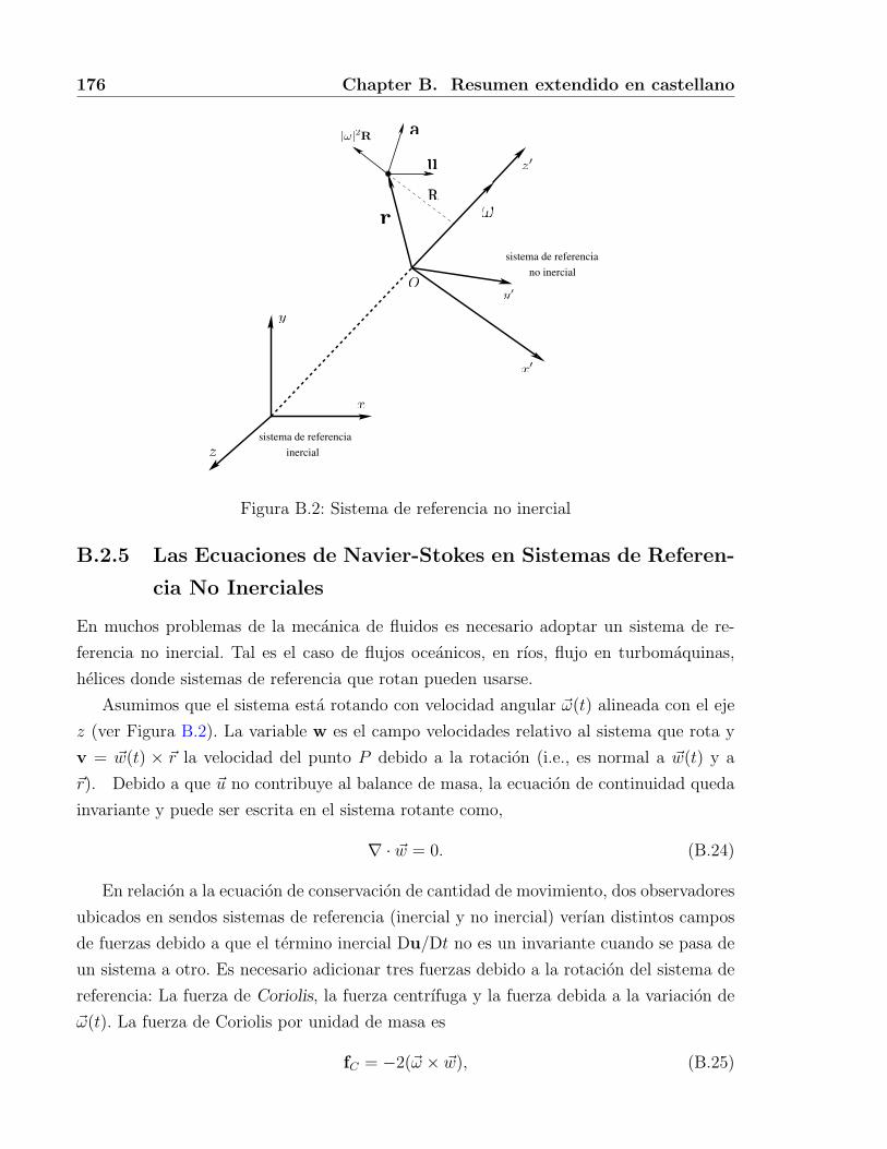
176 Chapter B. Resumen extendido en castellano
sistema de referenciainercial
sistema de referenciano inercial
y
x
z
|ω|2R
O
x′
y′
z′
r
R
u
a
ω
Figura B.2: Sistema de referencia no inercial
B.2.5 Las Ecuaciones de Navier-Stokes en Sistemas de Referen-
cia No Inerciales
En muchos problemas de la mecanica de fluidos es necesario adoptar un sistema de re-
ferencia no inercial. Tal es el caso de flujos oceanicos, en rıos, flujo en turbomaquinas,
helices donde sistemas de referencia que rotan pueden usarse.
Asumimos que el sistema esta rotando con velocidad angular ~ω(t) alineada con el eje
z (ver Figura B.2). La variable w es el campo velocidades relativo al sistema que rota y
v = ~w(t) × ~r la velocidad del punto P debido a la rotacion (i.e., es normal a ~w(t) y a
~r). Debido a que ~u no contribuye al balance de masa, la ecuacion de continuidad queda
invariante y puede ser escrita en el sistema rotante como,
∇ · ~w = 0. (B.24)
En relacion a la ecuacion de conservacion de cantidad de movimiento, dos observadores
ubicados en sendos sistemas de referencia (inercial y no inercial) verıan distintos campos
de fuerzas debido a que el termino inercial Du/Dt no es un invariante cuando se pasa de
un sistema a otro. Es necesario adicionar tres fuerzas debido a la rotacion del sistema de
referencia: La fuerza de Coriolis, la fuerza centrıfuga y la fuerza debida a la variacion de
~ω(t). La fuerza de Coriolis por unidad de masa es
fC = −2(~ω × ~w), (B.25)

B.2. Ecuaciones de Gobierno 177
la fuerza centrıfuga por unidad de masa es
fc = −~ω × (~ω × ~r) = |~ω|2 ~R, (B.26)
y la fuerza debido al cambio de ~ω(t) por unidad de masa
fr =d~ω(t)
dt= ~ω(t) = ~θ(t), (B.27)
La ecuacion de conservacion de momento queda ahora
∂uj
∂t+ uj
∂ui
∂xi
= −1
ρ
∂P
∂xj
+ ν∂2
∂xi∂xi
uj −∂p
∂xj
− ρ∂Ψ
∂xj
, ∀ (x, t) en V× (t0,∞). (B.28)
B.2.6 Las Ecuaciones de Navier-Stokes Incompresibles
Si consideramos el flujo de un fluido newtoniano incompresible (con propiedades constan-
tes), la ecuacion constitutiva se escribe de la forma
τij = −Pδij + µ
(∂ui
∂xj
+∂uj
∂xi
). (B.29)
Recordando que para fluidos incompresibles el campo de velocidades es solenoidal (i.e.,
∂ui/∂xi = 0), entonces la ecuacion constitutiva resulta de la suma de un termino isotropi-
co, −Pδij y de un termino deviatorico. La ecuacion de momento (B.22) se escribe
ρD
Dtuj = µ
∂2
∂xi∂xi
uj −∂p
∂xj
− ρ∂Ψ
∂xj
, ∀ (x, t) en V × (t0,∞). (B.30)
que es la ecuacion de Navier-Stokes (vectorial) para la conservacion de la cantidad de
movimiento. Si escribimos a la viscosidad cinematica como ν = µ/ρ, la ecuacion (B.30)
quedaD
Dtuj = ν
∂2
∂xi∂xi
uj −1
ρ
∂P
∂xj
− ∂Ψ
∂xj
, ∀ (x, t) en V × (t0,∞). (B.31)
Reescribiendo el lado izquierdo de la ecuacion (B.31), la forma Euleriana no conservativa
de la ecuacion de conservacion de la cantidad de movimiento queda
∂uj
∂t+ uj
∂ui
∂xi
= −1
ρ
∂P
∂xj
+ ν∂2
∂xi∂xi
uj −∂p
∂xj
− ρ∂Ψ
∂xj
, ∀ (x, t) en V× (t0,∞). (B.32)
Para que el problema quede bien planteado en el sentido de Hadamard ([Had02], ver
apendice §B.5) se deben definir condiciones para el vector velocidad en la frontera S(t)
del volumen V(t) e iniciales a las ecuaciones (B.31) y (B.32). Por ejemplo, en una pared
solida estacionaria cuyo vector normal unitario es n, las condiciones de borde que debe
satisfacer el campo de velocidades es la condicion de impermeabilidad
n · u = 0, ∀ (x, t) en S× (t0, tn), (B.33)

178 Chapter B. Resumen extendido en castellano
y la condicion de no deslizamiento
u− n(n · u) = 0, ∀ (x, t) en S× (t0, tn), (B.34)
(que de manera conjunta hacen u = 0 en la frontera). La condicion inicial es del tipo
u = u0, ∀ (x, t) en V × 0. (B.35)
Estas condiciones son del tipo mas simple que podemos plantear en este capıtulo, dejando
para posteriores capıtulos y secciones el tratamiento de condiciones de borde e iniciales
mas especiales, que se ajustan a distintos problemas y modelos (i.e., flujos turbulentos, pa-
redes moviles, condiciones de borde absorbentes, etc.). Tambien hay que agregar aquı que
se necesita la definicion de la presion P en un punto de V, debido a que esta variable debe
satisfacer una ecuacion de tipo elıptica como se vera mas adelante y la solucion para este
problema esta definido a diferencia de una constante.
En algunos casos puede ser interesante considerar el caso hipotetico de un fluido ideal
que no posee viscosidad (o es invıscido) para el cual el tensor de tensiones se define
isotropico (i.e., τij = −pδij). La ecuacion de conservacion de momento resultante es la
ecuacion de Euler incompresible
D
Dtuj = −1
ρ
∂p
∂xj
− ∂Ψ
∂xj
, ∀ (x, t) en V × (t0,∞). (B.36)
Debido a que estas ecuaciones no contienen derivadas segundas de la velocidad requieren
diferentes condiciones de borde que las ecuaciones de Navier-Stokes incompresibles. Por
ejemplo, en el caso una frontera solida estacionaria solo la condicion de impermeabilidad
puede verificarse, mientras que en general las velocidades tangenciales son distintas no
nulas.
El Rol de la Presion
El rol de la presion en las ecuaciones de Navier-Stokes incompresible (densidad constante)
requiere ser comentado. Primero hay que observar que las tensiones isotropicas y las fuer-
zas de volumen conservativas tienen el mismo efecto. Por lo tanto pueden ser agrupadas
dentro de un mismo termino (i.e., la presion modificada), p = P + ρΨ. Ası, las fuerzas de
volumen no tienen influencia sobre el campo de velocidades y sobre el campo de presiones
modificadas (en contraste con los flujos de fluido de densidad variable donde las fuerzas de
boyancia pueden resultar significantes). Por lo tanto, de aquı en adelante nos referiremos
simplemente a p como la ‘presion’.
Es costumbre tomar a la presion como una variable termodinamica que es funcion de
la densidad y de la temperatura a traves de una ecuacion de estado. Sin embargo, para

B.3. Formulacion de otros Modelos Matematicos a Tratar 179
fluidos con densidad constante no hay ninguna vinculacion con la densidad (ni con la
temperatura) y una vision distinta de esta variable es necesaria.
Si aplicamos el operador divergencia a las ecuaciones de Navier-Stokes, ecuacion (B.30),
sin asumir que el campo de velocidades es solenoidal pero denotando a ∆ como la dilata-
cion (o razon de dilatacion ∆ = ∇ · u), el resultado es(D
Dt− ν∇2
)∆ = R, (B.37)
siendo
R =1
ρ∇2p− ∂ui
∂xj
∂uj
∂xi
. (B.38)
Consideremos la solucion a la ecuacion (B.37) con condiciones iniciales y de contorno
∆ = 0. La solucion es ∆ = 0 si y solo si R es cero en todo V que a su vez implica (por la
ecuacion (B.38)) que p debe satisfacer la ecuacion de Poisson
∇2p = S ≡ −ρ∂ui
∂xj
∂uj
∂xi
. (B.39)
La verificacion de la ecuacion de Poisson es una condicion necesaria y suficiente para que
todo campo de velocidades solenoidal permanezca solenoidal.
En una pared solida estacionaria la ecuacion (B.30) se reduce a
∂p
∂n= µ
∂2un
∂n2, (B.40)
donde n es la coordenada en la direccion normal a la pared y un la proyeccion de la
velocidad sobre n. Esta ecuacion provee una condicion de borde del tipo Neumann para el
problema de Poisson (ecuacion (B.37)). Dada esta condicion y la ecuacion (B.37) queda
determinada la presion p a diferencia de una funcion constante ([Fol76]).
B.3 Formulacion de otros Modelos Matematicos a
Tratar
B.3.1 Problemas Hidrologicos
Se abordara tambien en esta tesis el desarrollo de un modulo de calculo en paralelo orien-
tado a objetos que sea capaz de modelar problemas (en una gran diversidad de escalas)
de hidrologıa superficial y subterranea acoplada∗ (proyecto PID-99/74 FLAGS de la
∗La importancia de la escala y la complejidad asociada de un modelo en hidrologıa fue abordada porDooge (1998), quien dijo que ‘en orden de predecir el comportamiento de una cuenca en forma confiable,

180 Chapter B. Resumen extendido en castellano
ANPCyT). Es necesario para esta parte del trabajo desarrollar/adaptadar herramientas
que no son estandar en mecanica de fluidos computacional y que resultan de gran impor-
tancia para el tratamiento de este tipo de problemas, como por ejemplo lo es la generacion
de mallas de calidad a partir de los modelos digitales de terrenos y la interpolacion de pro-
piedades fısicas a partir de datos medidos en campo que son necesarias en la modelacion.
Este desarrollo constituye una aporte original de la tesis.
Flujo Superficial
El flujo a superficie libre que escurre tanto sobre la superficie del terreno como concentrado
en canales abiertos, constituye la respuesta de dinamica mas rapida de una cuenca hıdrica
ante la solicitacion ocasionada por la precipitacion caıda en parte o en la totalidad de su
superficie.
Si L0 representa una longitud tıpica donde se observan variaciones apreciables en
la dinamica del escurrimiento, y h0 representa un espesor medio de la capa en dicha
distancia, la aproximacion de aguas poco profundas (u ondas largas) se basa en asumir
que h0/L0 1. Pueden derivarse las ecuaciones de Saint-Venant para el flujo en canales
abiertos a partir de las ecuaciones de Navier-Stokes integrando las variables en la direccion
vertical. Estas ecuaciones en la forma matricial conservativa resulta (la convencion de
Einstein para la suma es usada),
∂U
∂t+∂Fi(U)
∂xi
= Gi(U), i = 1, .., 3, sobre Ωst × (0, t], (B.41)
donde Ωst es el dominio de calculo (i.e., el rıo) y U = (h, hw, hv)T es el vector de estado.
Las funciones de flujo advectivo en la ecuacion (B.41) son
F1(U) = (hw, hw2 + gh2
2, hwv)T ,
F2(U) = (hv, hwv, hv2 + gh2
2)T ,
(B.42)
donde h es la altura de la superficie libre del canal con respecto al fondo del mismo,
u = (w, v)T es el vector velocidad y g es la aceleracion debida al campo gravitatorio. Si
Gs representa la recarga o las perdidas del rıo, el termino fuente es
G(U) = (Gs, gh(S0x−Sfx)+fchv+Cf$x|$|, gh(S0y−Sfy)−fchw+Cf$y|$|)T (B.43)
o bien debemos resolver modelos extremadamente complejos basados en las leyes fısicas de los procesos
involucrados, y que tengan en cuenta la variabilidad espacial de los diversos parametros, o bien debemos
resolver modelos realistas a escala de cuenca en los que el efecto global de esas propiedades variables en
el espacio este parametrizado de alguna manera’, enfatizando tambien la inexistencia de un principio desimilitud en hidrologıa que describa el comportamiento de una cuenca.
B.3. Formulacion de otros Modelos Matematicos a Tratar 181
donde S0 es la pendiente del fondo y Sf es la pendiente de friccion dada por
Sfx =1
Chhw|u|, Sfy =
1
Chhv|u|, Modelo de Chezy,
Sfx =n2
h4/3w|u|, Sfy =
n2
h4/3v|u|, Modelo de Manning,
(B.44)
donde Ch y n (la rugosidad de Manning) son constantes del modelo. Generalmente el
efecto de la fuerza de Coriolis, referida al factor de Coriolis fc, debe ser tenido en cuenta
cuando se estudian casos en grandes lagos, anchos rıos o estuarios. El factor de Coriolis
esta dado por fc = 2ω sinψ, donde ω es la velocidad de rotacion de la tierra y ψ es la
latitud del area en estudio. Las tensiones en la superficie libre en la ecuacion (B.43) son
expresadas como el producto entre un coeficiente de friccion y una forma cuadratica de
la velocidad de viento, $($x, $y), y
Cf = c$ρair
ρ, (B.45)
donde c$ es funcion de la velocidad del viento.
Flujo Subterraneo Saturado
La ecuacion de movimiento para el medio saturado parte de considerar la conservacion de
la masa. Si φ representa el potencial piezometrico en un punto del acuıfero, suma de la
energıa potencial gravitatoria mas la contribucion de la presion, la ecuacion de movimiento
del agua en el medio poroso se reduce a
∂
∂t(S(φ− η)φ) = ∇ · (K(φ− η)∇φ) +
∑Ga, sobre Ωaq × (0, t], (B.46)
donde Ωaq representa el dominio para el flujo subterraneo, η es una posicion de referencia
(datum), K representa el tensor de conductividades hidraulica y S el coeficiente de alma-
cenamiento especıfico que puede considerarse como la cantidad de agua almacenada que
se libera por unidad de volumen del acuıfero cuando el potencial disminuye una unidad.
Condiciones de Borde para Simular la Interaccion Rıo-Acuıfero/Termino de
Acople
El proceso de interaccion Rıo-Acuıfero ocurre entre un rıo (o canal, en general) y el
acuıfero adyacente. El termino de acople no esta incluido explıcitamente en la ecuacion
(B.46) pero se trata como una integral de flujo en el borde. En un punto nodal podemos
escribir el acople como
Gs = P/Rf (φ− hb − h), (B.47)
182 Chapter B. Resumen extendido en castellano
donde Gs representa la recarga o perdida del rıo al acuıfero adyacente, y Rf es el factor de
resistencia por unidad de longitud de arco del perımetro de la seccion. La correspondiente
recarga del acuıfero es
Ga = −Gs δΓs , (B.48)
donde Ga representa la curva del rıo (en el plano del acuıfero) y δΓs es una distribucion
delta de Dirac con una intensidad unitaria por unidad de longitud, es decir∫f(x) δΓs dΣ =
∫ L
0
f(x(s)) ds. (B.49)
Las ecuaciones (B.41) y (B.46) acopladas, con las condiciones de borde e iniciales apropia-
das, constituyen en sistema fuertemente acoplado no lineal de muy difıcil resolucion. El
acoplamiento se da a traves de las condiciones de borde que representan los mecanismos
de transferencia de masa entre cada subsistema. La solucion simultanea de las ecuaciones
no solo constituye un esfuerzo considerable de calculo sino que es computacionalmente
ineficiente puesto que ignora algunos rasgos fısicos esenciales de la interaccion entre los
subsistemas. El esquema de avance temporal adoptado constituye el algoritmo que mejor
refleja la competencia entre los mecanismos fısicos presentes en el sistema.
Por otra parte, la integracion vertical de la ecuacion de gobierno para el flujo sub-
terraneo tridimensional en cada una de las capas bajo la hipotesis de Dupuit lleva a una
ecuacion bidimensional promediada en la vertical, que es una de las aproximaciones que
se adoptaran en el trabajo.
B.4 Computacion de Alta Performance
B.4.1 Resolucion Numerica del Modelo de CFD/Hidrologıa Su-
perficial y Subterranea
El modelo se implementara en PETSc-FEM, un codigo de Elementos Finitos desarrollado
en el CIMEC de uso general y orientado a problemas multi-fısica (http://www.cimec.
org.ar/petscfem), escrito en C++ y basado en PETSc (‘Portable, Extensible Toolkit for
Scientific Computation’, http://www.mcs.anl.gov/petsc). PETSc es una librerıa de ruti-
nas orientadas a metodos numericos para la resolucion de Ecuaciones en Derivadas Par-
ciales (EDDP’s) y requiere alguna implementacion de la librerıa de paso de mensajes MPI
(Message Passing Interface). En nuestro caso usamos MPICH (http://www.mcs.anl.gov/mpi/mpich)
desarrollado en ANL (Argonne National Laboratory). El particionamiento de la malla es
un punto muy importante para una implementacion eficiente y sera realizado con METIS
(http://www.cs.umn.edu/ metis).
B.4. Computacion de Alta Performance 183
Consideraciones Generales
Si bien el problema matematico es bien conocido, las escalas de longitud y tiempo en juego
en problemas de hidrologıa hacen que los tiempos de calculo sean considerables y requieran
el uso de metodologıas especiales, como el empleo de calculo distribuido (paralelismo) y
metodos iterativos. De la misma manera en el tratamiento de flujos complejos (e.g., flujos
a altos Reynolds, a altos Mach y alrededor de cuerpos de variada geometrıa) mediante
las ecuaciones de Navier-Stokes es necesario utilizar modelos numericos que describan los
fenomenos turbulentos que se dan y para esto es necesario un alto grado de refinamiento
en las mallas (ademas de contar con la adaptacion de estas a las estructuras que se forman
en dichos regımenes) que se traduce en un problema de gran escala debido a la cantidad de
grados de libertad necesaria (en una simulacion DNS (por Direct Numerical Simulation)
de las ecuaciones de Navier-Stokes 3D incompresible son necesarios Re9/4 nodos con 4
grados de libertad por nodo para captar las estructuras turbulentas que se desarrollan).
El procesamiento distribuido (calculo en paralelo) usando clusters de PC’s de tipo
‘Beowulf’ permite abordar estos tipos de problemas a un costo bajo y con equipamiento
de gran accesibilidad (COTS = ‘Commodities-Off-The-Shelf’).
B.4.2 Solucion de Grandes Sistemas de Ecuaciones
La resolucion de grandes sistemas de ecuaciones algebraicas lineales subyace en la solucion
numerica de problemas de la mecanica del continuo y muchos otros problemas ingenie-
riles, llegando a constituir en muchos casos el principal factor de costo computacional.
Entre las plataformas de calculo, los clusters de microprocesadores han resultado ser una
alternativa muy eficiente y abordable para resolver grandes problemas numericos. Los
metodos clasicos de resolucion se suelen clasificar en directos o iterativos. Los primeros
proporcionan una solucion cerrada pero el principal inconveniente es el costo tanto en
tiempo de procesamiento como en almacenamiento en memoria. La cantidad de operacio-
nes requeridas para una matriz llena es del orden de n3, siendo n la cantidad de incognitas.
Los procedimientos iterativos son entonces preferidos para resolver sistemas grandes. Sin
embargo en grandes sistemas de ecuaciones el numero de condicion de la matriz empeora
y la solucion se dificulta. En la solucion iterativa se hace necesario precondicionar satis-
factoriamente la matriz del sistema de modo de poder obtener la solucion en un numero
razonable de iteraciones. Aun ası se han encontrado casos en que la solucion directamente
no es alcanzable. Hay tecnicas basadas en particionar el dominio y efectuar resoluciones
a niveles de las incognitas de cada subdominio y a nivel de aquellas en la interfaz entre
subdominios. Son las tecnicas de descomposicion de dominio que combinan resoluciones

184 Chapter B. Resumen extendido en castellano
directas e iterativas. Se requiere adecuados precondicionadores a fin de obtener resultados
satisfactorios.
Metodos Iterativos
Los metodos iterativos se basan en construir una secuencia de soluciones aproximadas
xk (k = 1, 2, . . .) tal que cuando el ındice de la iteracion k →∞ converja a la solucion
del sistema de ecuaciones.
Las formulas de recurrencia pueden presentarse de diferentes maneras. Por ejemplo se
puede plantear
xk = Gxk−1 + c (B.50)
que a partir de una estimacion inicial x0 permita obtener la solucion aproximada en
cada iteracion. Para que el metodo converja se requiere que ||G|| < 1. Clasicos metodos
iterativos como Jacobi, Gauss-Seidel o SOR pueden encuadrarse en esta tipologıa.
Procedimientos basados en optimizacion resultan eficientes para la resolucion iterativa
de sistemas de ecuaciones. Entre ellos, el metodo de gradientes conjugados (para matrices
simetricas) o GMRes (para matrices no simetricas) gozan de extendida popularidad. En
ellos las iteraciones se realizan en la forma
xk+1 = xk + αk pk (B.51)
a partir de una estimacion inicial x0. En cada paso es preciso calcular una direccion
de busqueda pk, con formulas propias de cada metodo, y un paso de avance αk en esa
direccion.
Estos metodos, basados en iteracion por subespacios, poseen buenas propiedades de
convergencia. No obstante, si el numero de condicion es alto (lo que tıpicamente sucede en
grandes problemas) es necesario introducir un precondicionamiento. Esto se discutira mas
adelante.
En el algoritmo de la Cuadro B.1 se indica el tipo de operacion a realizar. Los calculos
mas pesados son los relativos a producto de matriz por vector. Tambien es necesario
realizar producto interno de vectores y actualizacion de vectores (AXPY).
Si las matrices se distribuyen adecuadamente entre los procesadores, por bloques de
filas, el producto matriz por vector puede realizarse con independencia en cada procesador,
lo mismo que la actualizacion de vectores. El producto interno, sin embargo, requiere
comunicacion para realizar la operacion de reduccion y el posterior envıo del escalar
resultante a todos los procesadores.
La matriz del sistema de ecuaciones interviene en el proceso solamente al realizar
el producto matriz por vector. Es importante resaltar que no se precisa disponer de la
B.4. Computacion de Alta Performance 185
matriz global en ningun momento. Para efectuar el producto matriz por vector podrıan
utilizarse las matrices elementales del metodo de elementos finitos y ensamblarse el vector
resultante. Por otra parte la solucion iterativa contiene un error algorıtmico. El costo de
la solucion puede ajustarse segun la tolerancia especificada para el problema.
B.4.3 Metodos de Descomposicion de Dominio
Estos metodos se basan en descomponer el dominio de definicion del problema en sub-
dominios de modo que en cada uno de estos el problema sea mas facil de resolver (por
ejemplo si se lo resuelve analıticamente), o bien sea de un tamano adecuado para ser alo-
jado en un procesador. Estos subdominios pueden solaparse (metodo de Schwarz) o no.
Entre los que no se solapan, es decir el contacto se produce unicamente en las fronteras
inter-subdominio, se incluyen los procedimientos que utilizan el complemento de Schur.
El metodo de descomposicion de dominio puede mirarse como un buen procedimiento
para precondicionar el problema global. Como casos lımites se comporta como un proce-
dimiento directo cuando el tamano de los subdominios tiende a uno, o como un metodo
iterativo global cuando la frontera es extendida a todos los subdominios (no hay dominios
internos).
Matriz Complemento de Schur
Considerese una descomposicion como en la Figura B.3. Con Ωs se designa el subdominio
s (s = 1, Ns) y con Γsi (i = 1, 3) las fronteras del mismo. Aquı Γ1 se utilizara para
indicar el contorno con condiciones de tipo Dirichlet, Γ2 para aquel con condiciones de
tipo Neumann y Γ3 para las fronteras con otros subdominios (Figura B.3). Si se utiliza
el metodo de los elementos finitos, para resolver numericamente el problema en derivadas
parciales se llega a un sistema de ecuaciones
Ku = f , (B.52)
siendo u el vector de las variables nodales (velocidades y presiones en un problema de
fluidos, desplazamientos en un problema de solido deformable elastico), f es el vector de
variables discretas duales (fuerzas nodales), y K la matriz del sistema (rigidez).
Las matrices de la ecuacion (B.52) se construyen por subdominios y aquellas restrin-
gidas al subdominio s se designan por Ks, us y f s. Se pueden particionar en grupos de
incognitas (grados de libertad) internos al subdominio us y aquellos en la interfaz us. La

186 Chapter B. Resumen extendido en castellano
nlay = 2strip
21
interface (I)strip boundaries (SB)
internal layers (S)
Figura B.3: Descomposicion del Dominio
matriz de rigidez se puede escribir
Ks =
[Ks Ks
Ks,T Ks
](B.53)
y los vectores de desplazamientos y fuerzas nodales
us =
[us
us
]y f s =
[f s
f s
], (B.54)
El sımbolo 2 se usa aquı para grados de libertad internos, 2 para aquellos en la interfaz
y 2 para la interaccion entre ambos.
Si, por otra parte, se ensambla la contribucion de todos los subdominios a los grados
de interfaz globales, se puede escribir
KI =Ns
As=1
Ks, (B.55)
siendo uI el vector de desplazamientos en grados de libertad de interfaz de todo el dominio.
Las matrices con subındice I tienen el tamano del problema de interfaz global.
La ecuacion de equilibrio (B.52) se puede particionar en los siguientes sistemasKsus + ~Ks
IuI = f s , s = 1, Ns
Ns∑s=1
~Ks,TI us + KIuI = fI
(B.56)
B.4. Computacion de Alta Performance 187
y efectuando la eliminacion (gaussiana) por bloques
Ksus = f s − ~Ks
IuI , s = 1, Ns
[KI −Ns∑s=1
~Ks,TI (Ks)
−1 ~KsI ]uI = fI −
Ns∑s=1
~Ks,TI (Ks)
−1f s
(B.57)
La matriz de la segunda ecuacion en (B.57):
S = KI −Ns∑s=1
~Ks,TI (Ks)
−1 ~KsI (B.58)
se conoce como matriz complemento de Schur o matriz de capacitancia.
El primer grupo de ecuaciones en (B.57) representa el sistema asociado a los grados de
libertad internos us a cada subdominio, resultantes de la caracterıstica de no penetracion
de la descomposicion. Esta parte de la solucion es perfectamente paralelizable. El tamano
de estos problemas esta dado por la granularidad de la descomposicion en subdominios.
La segunda parte de la ecuacion (B.57) representa el problema de interfaz. El tamano
de la matriz complemento de Schur S es menor que el de la matriz global K, pero S
resulta densa. El numero de condicion de S es tambien menor que el de K. Por otra parte
no es necesario el ensamble explıcito de la matriz S, pudiendo efectuarse las operaciones
para la resolucion en cada subdominios. Esta parte de la solucion es acoplada para todo
el problema requiriendo comunicacion entre los distintos procesadores para su resolucion
en paralelo.
La solucion del problema (B.57) puede verse como efectuada en dos partes: un pro-
blema de grados de libertad de interfaz y otro de grados de libertad internos a los subdo-
minios. Se suele resolver el problema interno a traves de metodos directos y el problema
en la interfaz mediante tecnicas iterativas. El uso de metodos directos para los proble-
mas internos evita errores algorıtmicos que se propaguen al problema de interfaz. Como
el tamano de los problemas internos es acotado al subdominio los metodos directos son
aplicables.
Para el problema de interfaz, sin embargo, un metodo directo no es atractivo, por
los requerimientos de almacenamiento. La matriz S es una matriz completa y cara para
construir. Por este motivo se suele recurrir a metodos iterativos (Gradiente conjugado,
GMRes) con un adecuado precondicionamiento. La descomposicion de dominio brinda un
adecuado precondicionamiento para el problema global.

188 Chapter B. Resumen extendido en castellano
Solucion Iterativa del Problema de Interfaz
La submatriz de rigidez asociada a los grados de libertad de interfaz KI puede escribirse
KI =Ns∑s=1
KsI (B.59)
y la matriz complemento de Schur
S =Ns∑s=1
Ss, (B.60)
donde
Ss = KsI − ~Ks,T
I (Ks)−1 ~Ks
I . (B.61)
La ecuacion (B.60) muestra que la contribucion de cada subdominio a la matriz S puede
calcularse independientemente. La ecuacion (B.57-b) puede ser re-escrita
S uI = gI (B.62)
La solucion de la ecuacion (B.62) por un metodo iterativo (GMRes para el caso de ope-
radores no simetricos y/o no definidos positivos, gradiente conjugado para el caso de
operadores simetricos como ocurre en elasticidad lineal) se puede realizar con un algorit-
mo como el de la Cuadro B.1. Allı se considera un sistema generico
Ax = b (B.63)
y se realiza ademas un precondicionamiento con la intencion de bajar el numero de con-
dicion de la matriz.
Puede observarse que las fases del proceso que resultan mas demandantes en tiempo
de procesamiento son el producto matriz-vector en los pasos I.2 y II.2, y la solucion del
sistema de ecuaciones implıcita en el precondicionamiento, en los pasos I.3 y II.7. Las
restantes operaciones sobre vectores, del tamano del problema de interfaz global, son
productos internos y actualizacion de vectores (AXPY).
B.4.4 Precondicionamiento
El precondicionamiento resulta indispensable para la resolucion de grandes sistemas de
ecuaciones por tecnicas iterativas. Existen varios procedimientos para precondicionamien-
to. Entre ellos pueden mencionarse:

B.4. Computacion de Alta Performance 189
Cuadro B.1: Algoritmo Gradiente Conjugado Precondicionado
I. Inicializacion
I.1 x estimacion inicial
I.2 r = b−Ax matriz × vector + suma vect.
I.3 solve Pz = r solucion sistema
I.4 ρ = (r, z) producto interno
I.5 ρ0 = ρ
I.6 p = z
I.7 k = 1
II. Iterar: mientras k < Kmax hacer
II.1 Test de Convergencia: si ρ < Tol ρ0 finaliza iteraciones
II.2 a = Ap matriz × vector
II.3 m = (p, a) producto interno
II.4 α = ρm
II.5 x = x + αp AXPY
II.6 r = r− αa AXPY
II.7 resolver Pz = r solucion sistema
II.8 ρold = ρ
II.9 ρ = (r, z) producto interno
II.10 γ = ρρold
II.11 p = z + γp AXPY
II.12 k = k + 1, ir a II.1
1. Jacobi o escalado diagonal
Este es el mas simple y se basa en tomar como precondicionador la matriz
P = diag(A). (B.64)
No requiere resolver sistema alguno, pero solamente es eficiente si la matriz del
sistema es diagonal dominante.
2. Factorizacion incompleta En este caso la factorizacion LU, o la factorizacion de
Cholesky CTC para el caso de matrices simetricas positiva definidas, se efectua

190 Chapter B. Resumen extendido en castellano
pero deteniendo el proceso al alcanzar la estructura rala de la matriz A. Se propone
entonces como precondicionador:
P = LTU (B.65)
siendo L y U los factores incompletos. Este precondicionador podrıa llevar a te-
ner pivotes nulos. Se han introducido modificaciones tales como Shifted Incomplete
Cholesky Factorization para eliminar este problema.
Metodo Neumann-Neumann
Si se observa el algoritmo de la Cuadro B.1 se puede ver que las partes que demandan
mayor tiempo de procesamiento son, como se ha indicado, el producto matriz-vector en los
pasos I.2 y II.2, y la solucion del sistema de ecuaciones implıcita en el precondicionamiento,
en los pasos I.3 y II.7.
El producto matriz por vector (I.2 y II.2) puede escribirse
a = Sp, (B.66)
siendo S la matriz complemento de Schur y, debido a (B.60),
a =Ns∑s=1
as =Ns∑s=1
Ssp, (B.67)
Esto es, las contribuciones a a se calculan separadamente en cada subdominio. En el
subdominio s se tiene (B.61)
Ssp = [KsI − ~Ks,T
I (Ks)−1 ~Ks
I ]p (B.68)
y considerando el problema restringido al subdominio[Ks ~Ks
~Ks,T KsI
][vs
p
]=
[0
as
]. (B.69)
La contribucion del subdominio s al vector (B.67) es
as = ~Ks,Tvs + Ksip, (B.70)
siendo vs solucion de
Ksvs = −~Ksp. (B.71)
Las ecuaciones (B.69) a (B.71) muestran que para evaluar el producto matriz-vector (B.67)
basta con resolver, en cada subdominio, un problema de Dirichlet donde valores prescriptos

B.4. Computacion de Alta Performance 191
de p se impone en la interfaz Γs3, y se obtiene el vector asociado as. Finalmente se suman
las contribuciones as de cada subdominio.
Para realizar el precondicionamiento se efectua el siguiente procedimiento. En cada
subdominio se define una matriz DsI de modo que
Ns∑s=1
DsI = II . (B.72)
Esto significa que ensamblando las matrices DsI de todos los subdominios se obtiene la
matriz identidad en el espacio de interfaz global. La manera mas simple de construir DsI
es con una matriz diagonal cuyos terminos son la inversa de la cantidad de subdominios
que comparten el grado de libertad en cuestion.
En cada iteracion del gradiente conjugado, el residuo se proyecta sobre cada subdo-
minio
rs = Ds,T r (B.73)
y en cada subdominio se resuelve el sistema
Sszs = rs (B.74)
Finalmente las contribuciones de cada subdominio al vector z se promedian sobre la
interfaz
z =Ns∑s=1
Dszs (B.75)
Esto es equivalente a usar un precondicionamiento de la forma
P−1 =Ns∑s=1
Ds(Ss)−1DsT . (B.76)
La solucion de (B.74), a su vez, es equivalente a resolver el problema de Neumann en
el subdominio s, donde el vector solucion zs contiene, en un problema elastico, desplaza-
mientos de los grados de libertad de interfaz. Puede ser realizado sin formar explıcitamente
la matriz del complemento de Schur S, escribiendo para cada subdominio[Ks Ks
Ks,T KsI
][vs
zs
]=
[0
rs
]. (B.77)
La solucion del problema de Neumann (B.77) en el subdominio s es
vs = −(Ks)−1 ~Kszs (B.78)

192 Chapter B. Resumen extendido en castellano
zs =(Ks
I − ~Ks,T (Ks)−1 ~Ks
)−1rs =
(Ss)−1
rs. (B.79)
Cuando se resuelve iterativamente el problema de interfaz el producto matriz-vector (I.2
y II.2) y la solucion del sistema de ecuaciones (I.3 y II.7) se reemplazan por resoluciones
del problema restricto a cada subdominio, alternativamente con condiciones de Dirichlet o
de Neumann, respectivamente. Estas soluciones por subdominio resultan bien escalables.
Para un problema de Laplace mientras el numero de condicion de la matriz global es
O( 1h2 ) (siendo h el tamano de los elementos) aquel para el complemento de Schur es O( 1
h),
y utilizando el precondicionador (B.76) se reduce a O(1).
En general, en un problema de elasticidad, la ecuacion (B.74), sobre un subdominio,
posee a una matriz S singular a menos que se restrinjan suficientes grados de libertad
para impedir movimientos de cuerpo rıgido. Diversas tecnicas han sido desarrolladas para
eliminar este inconveniente en los subdominios ‘flotantes’.
Precondicionador de Franja alrededor de la Interfaz (‘Interface Strip Precon-
ditioner’)
El precondicionador propuesto aquı (y que se describe en el capıtulo §2) esta basado en
resolver un problema de Dirichlet alrededor de una franja (strip) de nodos alrededor de
la interfaz entre subdominios. Cuando el ancho de la franja es pequeno, el costo compu-
tacional y la demanda de memoria para resolver el problema de la interfaz son bajos y
el numero de iteraciones para converger a una dada tolerancia es relativamente alto. Lo
contrario sucede cuando el ancho de la interfaz es aumentada. La formulacion matematica
de este nuevo precondicionador y su aplicacion en la solucion de problemas en CFD son
expuestas en la tesis.
Este precondicionador resulta tener mejor desempeno para matrices que son resultado
de la discretizacion de operadores simetricos y ademas carece del problema de dominios
flotantes (modos rıgidos) como por ejemplo ocurre con el clasico precondicionador de
Neumann-Neumann. Se hace hincapie que para operadores que implican derivadas de las
incognitas (e.g., ecuacion de Laplace, elasticidad estacionaria, adveccion-difusion estacio-
naria) una parte de la frontera deberıa tener condiciones de tipo Dirichlet o mixtas. De
otra manera el problema esta mal planteado y la matriz resulta singular. Para el precon-
dicionador de Neumann-Neumann los subdominios heredan las condiciones del problema
original en la frontera externa, mientras que condiciones de Neumann son impuestas en
las fronteras de los subdominios interiores. Ası, subdominios que tienen interseccion vacıa
con la porcion de la frontera externa con condiciones Dirichlet y/o mixtas tendrıan condi-

B.4. Computacion de Alta Performance 193
ciones Neumann en toda la frontera y consecuentemente aparecerıan modos rıgidos para
los operadores descriptos anteriormente.
En contraste con otros precondicionadores, e.g., precondicionadores del tipo ‘wire-
basket’ [BPS86], el precondicionador de interfaz es puramente algebraico y puede ser
ensamblado a partir de un subconjunto de los coeficientes de la matriz. Ademas no hay
restricciones en cuanto a la topologıa de la malla y mas aun puede ser aplicado a ma-
trices ralas que provienen de otro tipo de problemas, no necesariamente de ecuaciones
diferenciales en derivadas parciales.
Consideremos la interfaz que resulta de la descomposicion de la Figura B.3 con una
franja de dos capas de elementos a cada lado (nlay = 2). El precondicionamiento consiste
en, dado el vector fI definido en los nodos en la interfaz (I en la Figura B.3) calcular vI
dado por el siguiente problema KII KIS KI,SB
KSI KSS KS,SB
KSB,I KSB,S KSB,SB
vI
vS
vSB
=
fI
0
0
, (B.80)
con ‘condiciones Dirichlet’ en las fronteras de la franja vSB = 0, tal que el problema se
reduce a [KII KIS
KSI KSS
][vI
vS
]=
[fI
0
]. (B.81)
Una vez que el sistema es resuelto, vI es el valor del precondicionador aplicado a fI , por
lo tanto
vI = P−1IS fI . (B.82)
B.4.5 Implementacion Operativa del Cluster
El cluster responde a la filosofıa Beowulf (http://www.beowulf.org/) desarrollado en el
CESDIS del Goddard Space Flight Center (GSFC-NASA). Existen una gran cantidad de
clusters de este tipo, que van desde unos pocos nodos hasta 1000 o mas (500 P-II duales,
http://www.genetic-programming.com/).
En nuestro caso se ha construido un cluster de 20 procesadores Intel P-IV, 2.8Ghz, con
2Gb RAM conectados entre sı por una red Fast Ethernet (100 Mbit/sec) soportado por
un switch Encore ENH924-AUUT+. La configuracion responde a la metodologıa disk-less,
es decir que los nodos no cuentan con monitor, teclado ni disco duro. Al bootear el nodo
carga el Sistema Operativo de un diskette, envıa un ‘RARP request’ al server y monta el
root filesystem via NFS (Network File System) en el disco del server.

194 Chapter B. Resumen extendido en castellano
El CIMEC ha proyectado construir ademas un cluster de alrededor 100 nodos (proyecto
PME 209 ANPCyT) donde se debera prestar especial atencion a la escalabilidad del
codigo generado.
B.5 Algunas Definiciones Topologicas
B.6 Dominio Lipschitz, Frontera Lipschitz
Un dominio abierto Ω es llamado ‘dominio Lipschitz’ y su frontera, ‘frontera Lipschitz’,
si esta conectado y si para cada punto en su frontera , x ∈ ∂Ω := Ω\Ω, existe una
transformacion de coordenadas Φ : Rd → Rd, a δ > 0, y una funcion Lipschitz-continua
η : [−δ,+δ]d−1 → R tal que
Ω ∩B(x, δ) = Φ(y1, ..., yd) ∈ B(x, δ) : η(y1, ..., yd) > yd
∂Ω ∩B(x, δ) = Φ(y1, ..., yd) ∈ B(x, δ) : η(y1, ..., yd) = yd
B(x, δ)\Ω = Φ(y1, ..., yd) ∈ B(x, δ) : η(y1, ..., yd) < yd,
(B.83)
donde B(x, δ) es una bola abierta de radio δ centrada en x. Un conjunto cerrado es llamado
‘dominio Lipschitz’ (cerrado) si es el cierre de un dominio Lipschitz (abierto). Un dominio
es un dominio Lipschitz si localmente su frontera puede ser representada como un grafo
de una funcion Lipschitz y si el dominio esta localmente a un lado de la frontera.
Figura B.4: Rudolf Otto Sigismund Lipschitz (1832–1903)
B.7. Funcion Lipschitz 195
B.7 Funcion Lipschitz
Sea f(t, x) una funcion continua por tramos en t. Si f satisface
||f(t, x)− f(t, y)|| ≤ L||x− y|| (B.84)
∀x, y ∈ B(x, δ) y ∀t ∈ [t0, t0 + β], β > 0, se dice que f es Lipschitz-continua en x o que
satisface continuamente la condicion de Lipschitz en x y L es la constante de Lipschitz.
Se dice que f(x) es localmente Lipschitz en un dominio (conjunto abierto y conexo)
D ⊂ Rn si cada punto de D tiene un entorno B(x, δ) tal que f satisface (B.84) con alguna
constante de Lipschitz L0. Tambien f(x) es Lipschitz en un conjunto W si satisface (B.84)
en todos los puntos deW , con la misma constante de Lipschitz L. Toda funcion localmente
Lipschitz en un dominioD es Lipschitz en todo subconjunto compacto (cerrado y acotado)
deD. Decimos que f(x) es globalmente Lipschitz si es Lipschitz en Rn. Decimos que f(t, x)
es localmente Lipschitz en x en [a, b]×D ⊂ R×Rn si cada punto x ⊂ D tiene un entorno
D0 tal que f satisface (B.84) en [a, b]×D0 con alguna constante de Lipschitz L0. Se dice
que f(t, x) es localmente Lipschitz en x en [t0,∞) × D si es localmente Lipschitz en x
en [a, b]×D para todo intervalo compacto [a, b] ⊂ [t0,∞). Tambien se dice que f(t, x) es
Lipschitz en [a, b]×W si satisface (B.84) para todo t ⊂ [a, b] y todo punto en W , con la
misma constante de Lipschitz L.
B.8 Problemas Bien Planteados en el Sentido de Ha-
damard
El termino matematico ‘problema bien planteado’ es debido a la definicion que diera
Hadamard en su artıculo de 1902 [Had02]. Hadamard decıa que los modelos matematicos
de los fenomenos fısicos debıan tener las siguientes propiedades,
i) La solucion debe existir,
ii) ser unica
iii) y depender en forma continua de los datos en una topologıa razonable.
Ejemplos de este tipo de problemas bien planteados son el problema de Dirichlet para la
ecuacion de Laplace y la ecuacion de la transmision no estacionaria de calor con condicio-
nes iniciales especificadas. Estos deben ser vistos como problemas ’naturales’ ya que hay
procesos fısicos que son descriptos por esas ecuaciones.
En contraste la ecuacion del calor integrada temporalmente hacia atras para determi-
nar una distribucion de temperatura, en tiempos previos, a partir de la distribucion final,

196 Chapter B. Resumen extendido en castellano
es un problema mal planteado ya que la solucion es altamente dependiente del estado
final. Los problemas inversos a menudo son mal planteados.
Problemas que surgen en la mecanica del continuo son discretizados para obtener solu-
ciones numericas (muy a pesar de algunos cientıficos) y en terminos del analisis funcional
resultan continuos. Si embargo pueden ‘sufrir’ de inestabilidades numericas cuando son
resueltos con precision finita o errores en los datos. Una medida del ‘buen planteamiento’
de un problema lineal discreto es el numero de condicion
Si un problema esta bien planteado se espera que la solucion sea la adecuada cuan-
do es resuelto en una computadora con precision finita usando un algoritmo estable. Si
no esta bien planteado es necesario que sea re-formulado para su resolucion numerica.
Tıpicamente son necesarias otras condiciones como las de regularidad o suavidad de la
solucion.

Bibliography
[Ali94] S.K. Aliabadi. Parallel finite element computations in aerospace applications.
phd. thesis. Department of Aerospace Engineering and Mechanics, University
of Minnesota, 1994.
[ARF84] S.R. Ahmed, G. Ramm, and G. Faltin. Some salient features of the times-
averaged ground vehicle wake. SAE Society of Automotive Eng., Inc.,
1(840300):1–31, 1984. 92, 94
[Arn51] W.E. Arnoldi. The principle of minimized iterations in the solution of the
matrix eigenvalue problem. Quarterly of Applied Mathematics, 9:17–29,
1951. 6
[ART93] S. Aliabadi, S. Ray, and T. Tezduyar. SUPG finite element computation of
viscous compressible flows based on the conservation and entropy variables
formulations. Computational Mechanics, 11:300–312, 1993. 54, 58
[BCHM86] M. Braza, P. Chassaing, and H. Ha Minh. Numerical study and physical
analysis of the pressure and velocity fields in the near wake of a circular
cylinder. Journal of Fluid Mechanics, 164:79–130, 1986. 82, 83, 85
[Bel99] A. Belmonte. Flutter and tumble in fluids. Physics World, 1999. 124
[BEM98] A. Belmonte, H. Eisenberg, and E. Moses. From flutter to tumble: Iner-
tial drag and froude similarity in falling paper. Physical Review Letters,
81(2):345–348, 1998.
[BGCMS04] S. Balay, W.D. Gropp, L. Curfman McInnes, and B.F. Smith. PETSc 2.2.0
user’s manual. Argonne National Laboratory, 2004. xiii, xvii, 49, 169
[BH82] A.N. Brooks and T.J.R. Hughes. Streamline upwind/petrov-galerkin for-
mulations for convection dominated flows with particular emphasis on the
197

198 BIBLIOGRAPHY
incompressible navier-stokes equations. Computer Methods in Applied Me-
chanics and Engineering, 32:199–259, 1982. 54, 170
[BLST90] M. Behr, J. Liou, R. Shih, and T.E. Tezduyar. Vorticity-stream function
formulation of unsteady incompressible flow past a cylinder: sensitivity of the
computed flow field to the location of the downstream boundary. University
of Minnesota Supercomputer Institute Research Report, UMSI 90/87, 1990.
82, 85
[BPS86] J.H. Bramble, J.E. Pasciak, and A.H. Schatz. The construction of precon-
ditioners for elliptic problems by substructuring, I. Mathematics of Compu-
tation, 47(175):103–134, 1986. xii, xvi, 14, 169, 193
[BPS89] J.H. Bramble, J.E. Pasciak, and A.H. Schatz. The construction of pre-
conditioners for elliptic problems by substructuring, IV. Mathematics of
Computation, 53(187):1–24, 1989. xii, 14
[BR92] J. Broeze and J.E. Romate. Absorbing boundary conditions for free surface
wave simulations with a panel method. Journal of Computational Physics,
99:146, 1992. 103
[BR96] F. Bourquin and N. Rabah. Decoupling and modal synthesis of vibrating
continuos systems. In 9th International Conference on Domain Decomposi-
tion Methods, 1996. 24
[Bre74] F. Brezzi. On the existence, uniqueness and approximation of saddle-point
problems arising from lagrangian multipliers. Rev. Francaise Automat.
Informt. Recherche Operationnelle Ser. Rouge Anal. Numer, R-2:129–151,
1974. 170
[BSI92] C. Baumann, M.A. Storti, and S.R. Idelsohn. Improving the convergence rate
of the petrov-galerkin techniques for the solution of transonic and supersonic
flows. International Journal for Numerical Methods in Engineering, 34:543–
568, 1992. 109
[Car72] J.E. Carter. Numerical solutions of the Navier-Stokes equations for the
supersonic laminar flow over two-dimensional compression corner. National
Aeronautics ans Space Administration (NASA), Thechnical Report R-385,
1972. 53

BIBLIOGRAPHY 199
[Ceb96] J. Cebral. Loose Coupling Algorithms for fluid structure interaction. PhD
thesis, Institute for Computational Sciences and Informatics, George Mason
University, 1996. 125
[Cho67] A.J. Chorin. Numerical method for solving incompressible viscous problems.
Journal of Computational Physics, 2(12), 1967.
[Cho73] A.J. Chorin. Numerical study of slightly viscous flow. Journal of Fluid
Mechanics, 57:785–796, 1973. 82, 170
[Cod01] R. Codina. Pressure stability in fractional step finite element methods for
incompressible flows. Journal of Computational Physics, 170:112–140, 2001.
87
[Cro02] J.M. Cros. A preconditioner for the Schur complement domain decomposi-
tion method. In 14th International Conference on Domain Decomposition
Methods, 2002. xvi, 24, 27, 169
[CW92] X.C. Cai and O.B. Widlund. Domain decomposition algorithms for indefinite
elliptic problems. SIAM Journal on Scientific Statistic Computing, 13:243–
258, 1992. 46
[DCC+95] E. Dowell, E. Crawley, H. Curtiss, D. Peters, R. Scanlan, and F. Sisto. A
Modern Course in Aeroelasticity. Kluwer Academic Publishers, Dordrecht,
1995. 132, 144
[DP06] W. Dettmer and D. Peric. A computational framework for fluid-rigid body
interaction: Finite element formulation and applications. Computer Methods
in Applied Mechanics and Engineering, 195:1633–1666, 2006. 132
[DW87] M. Dryja and 0. Widlund. An additive variant of the schwarz alternating
method for the case of many subregions. Technical Report 339, Courant
Institute of Mathematical Sciences, 1987. 46
[FKMN97] S. Field, M. Klaus, M. Moore, and F. Nori. Instabilities and chaos in falling
objects. Nature, 387:252–254, 1997. 124
[FLLT+01] C. Farhat, M. Lesoinne, P. Le Tallec, K. Pierson, and D. Rixen. FETI-DP: a
dual-primal unified FETI method-part I: A faster alternative to the two-level
FETI method. International Journal for Numerical Methods in Engineering,
50:1523–1544, 2001. 25

200 BIBLIOGRAPHY
[FM98] C. Farhat and J. Mandel. The two-level FETI method for static and dynamic
plate problems. Computer Methods in Applied Mechanics and Engineering,
155:129–152, 1998. 25
[FMR94] C. Farhat, J. Mandel, and F.X. Roux. Optimal convergence properties of
the FETI domain decomposition method. Computer Methods in Applied
Mechanics and Engineering, 115:365–385, 1994. 25
[Fol76] G.B. Folland. Introduction to partial differential equations. Princeton Uni-
versity Press-Uni, 1976. 179
[FPF01] C.A. Felippa, K.C. Park, and C. Farhat. Partitioned analysis of coupled me-
chanical systems. Computer Methods in Applied Mechanics and Engineering,
190:3247–3270, 2001. 132
[FR91] C. Farhat and F.X. Roux. A method of finite element tearing and inter-
connecting and its parallel solution algorithm. International Journal for
Numerical Methods in Engineering, 32:1205–1227, 1991. 25
[GGS82] U. Ghia, K.N. Ghia, and C.T. Shin. High-re solutions for incompressible
flow using the Navier-Stokes equations and a multigrid method. Journal of
Computational Physics, 48:387–411, 1982. 86
[GK89] D. Givoli and J.B. Keller. A finite element method for large domains. Com-
puter Methods in Applied Mechanics and Engineering, 76:41–66, 1989. 103
[GK90] D. Givoli and J.B. Keller. Non-reflecting boundary conditions for elastic
waves. Wave Motion, 12:261–279, 1990. 103
[GLD94] F. Grasso, G. Leone, and J. Delery. Validation procedure for the analysis of
shock-wave/boundary-layer interaction problems. AIAA Journal, 32,9:1820–
1827, 1994. 60
[GLS94] W. Gropp, E. Lusk, and A. Skjellum. Using MPI: Portable Parallel Pro-
gramming with the Message-Passing Interface. 2nd edition. The MIT Press,
London, England, 1994. xiii, xvii, 49, 169
[GR05] V. Gnesin and R. Rzadkowski. A coupled fluid structure analysis for 3-d
inviscid flutter of IV standard configuration. Jornal of Sound and Vibration.,
49:349–369, 2005. 132
BIBLIOGRAPHY 201
[Had02] J. Hadamard. Sur les problemes aux derivees partielles et leur signification
physique. Princeton University Bulletin, pages 49–52, 1902. 177, 195
[Hag87] T. Hagstrom. Boundary conditions at outflow for a problem with transport
and diffusion. Journal of Computational Physics, 69:69–80, 1987. 103
[HH92] I. Harari and T.J.R. Hughes. Galerkin least-squares finite element methods
for the reduced wave equation with non-reflecting boundary conditions in
unbounded domains. Computer Methods in Applied Mechanics and Engi-
neering, 98:411–454, 1992. 103
[Hir90] C. Hirsch. Numerical Computation of Internal and External Flows - Vol. II.
Wiley Series in Numerical Methods in Engineering., 1990. 55, 65
[Hou58] J.C. Houbolt. A study of several aerothermoelastic problems of aircraft
structures. Mitteilung aus dem Institut fur Flugzeugstatik und Leichtbau
5, E.T.H., Zurich, Switzerland, 1958. 139
[HS52] M.R. Hestenes and E. Stiefel. Methods of conjugate gradients for solving
linear systems. Journal of Research of the National Bureau of Standards,
49:409–436, 1952. 12
[HT84] T. Hughes and T. Tezduyar. Finite element methods for first-order hy-
perbolic systems with particular emphasis on the compressible euler equa-
tions. Computer Methods in Applied Mechanics and Engineering, 45:217–
284, 1984.
[Hua00] J.Y. Huang. Trajectory of a moving curveball in viscid flow. In Proceedings
of the Third International Conference: Dynamical Systems and Differential
Equations, pages 191–198, 2000. 124
[Hua01] J.Y. Huang. Moving Boundaries VI, chapter Moving Coordinates Methods
and Applications to the Oscillations of a Falling Slender Body, pages 73–82.
WIT Press, 2001. 124
[Hua02] J.Y. Huang. Advances in Fluid Mechanics IV, chapter Aerodynamics of a
Moving Curveball in Newtonian Flow, pages 597–608. WIT Press, 2002. 124
[KD03] S. Krajnovic and L. Davidson. Numerical study of the flow around the bus-
shaped body. Journal of Fluids Engineering, ASME, 125:500–509, 2003.
92

202 BIBLIOGRAPHY
[Kel95] C.T. Kelley. Iterative Methods for Linear and Nonlinear Equations. Frontiers
in Applied Mathematics, Vol. 16, SIAM, 1995. 11, 43
[KK03] J. Koo and C. Kleinstreuer. Liquid flow in microchannels: experimental
observations and computational analyses of microfluidics effects. Journal of
Micromechanics and Microengineering, 13:568–579, 2003. 74
[Lan50] C. Lanczos. An iteration method for the solution of the eigenvalue problem of
linear differential and integral operators. Journal of Research of the National
Bureau of Standards, 45(4):255–282, 1950. 6
[LC96] R. Lohner and J.R. Cebral. Fluid-structure interaction in industry: Issues
and outlook. In Proc. World User Association in Applied Computational
Fluid Dynamics, 3rd World Conference in Applied Computational Fluid Dy-
namics, Germany, May 19-23, 1996. 125
[LC98a] R. Lohner and J.R. Cebral. Fluid-structure-(thermal) interaction in indus-
try: Issues and outlook. In Proc. 4th World Conference and Exhibition in
Applied Fluid Dynamics, Freinurg i. Br., Germany, June 7-11, 1998.
[LC98b] R. Lohner and J.R. Cebral. Loads transfer for viscous fluid-structure inter-
action. In Proc. IV World Congress in Computational Mechanics, Buenos
Aires, Argentina, June 29-July 2, 1998.
[Lef05] E. Lefrancois. Numerical validation of a stability model for a flexible over-
expanded rocket nozzle. International Journal for Numerical Methods in
Fluids, 49:349–369, 2005. 132
[LMPV87] R. Lohner, K. Morgan, J. Peraire, and M. Vahdati. Finite element flux-
corrected transport (FEM-FCT) for the euler and navier-stokes equations.
International Journal for Numerical Methods in Engineering, pages 1093–
1109, 1987.
[LNST06] E. Lopez, N.M. Nigro, M.A. Storti, and J. Toth. A minimal element distor-
tion strategy for computational mesh dynamics. International Journal for
Numerical Methods in Engineering, 2006. 135
[LTV97] P. Le Tallec and M. Vidrascu. Solving large scale structural problems on par-
allel computers using domain decomposition techniques. In M. Papadrakakis,
editor, Parallel Solution Methods in Computational Mechanics, chapter 2,
pages 49–85. John Wiley & Sons Ltd., 1997. xi, xii, xv, 14, 17, 41, 167
BIBLIOGRAPHY 203
[LYC+98] R. Lohner, C. Yang, J.R. Cebral, J. Baum, H. Luo, D. Pelessone, and
C. Charman. Fluid-structure interaction using a loose coupling algorithm
and adaptive unstructured grids. AIAA paper AIAA-98-2419, 1998. 125
[LYC+00] R. Lohner, C. Yang, J.R. Cebral, J.D. Baum, H. Luo, E. Mestreau, and
E. Pelessone Charman. Fluid-structure interaction algorithms for rupture
and topology change. In Japan, 2000.
[Man93] J. Mandel. Balancing domain decomposition. Communications on Numerical
Methods in Engineering, 9:233–241, 1993. xvi, 24, 27, 38, 41, 169
[Meu99] G. Meurant. Computer Solution of Large Linear Systems, volume 28. Studies
in Mathematics and Its Applications. North-Holland, 1999. xvi, 14
[MRS99] L. Mahadevan, W.S. Ryu, and A.D.T. Samuel. Tumbling cards. Physics
Fluids, 11(1):1–3, 1999.
[Nor01] C. Norberg. Flow around a circular cylinder: Aspects of fluctuating lift.
Journal of Fluids and Structures, 15:459–469, 2001. 82
[NSI97] N.M. Nigro, M.A. Storti, and S.R. Idelsohn. GMRes physics based precondi-
tioner for all reynolds and mach number. numerical examples. International
Journal for Numerical Methods in Fluids, 25:1–25, 1997.
[PF00] K.C. Park and C.A. Felippa. A variational principle for the formulation of
partitioned structural systems. International Journal for Numerical Methods
in Engineering, 47:395–418, 2000. 132
[PF01] R. Piperno and C. Farhat. Partitioned procedures for the transient solu-
tion of coupled aeroelastic problems. Part II: energy transfer analysis and
three-dimensional applications. Computer Methods in Applied Mechanics
and Engineering, 190:3147–3170, 2001. 132, 135, 137, 138, 156
[PNS06] R.R. Paz, N.M. Nigro, and M.A. Storti. On the efficiency and quality of
numerical solutions in CFD problems using the interface strip preconditioner
for domain decomposition methods. International Journal for Numerical
Methods in Fluids, 52(1):89–118, 2006. xi, 14, 80
[PS05] R.R. Paz and M.A. Storti. An interface strip preconditioner for domain
decomposition methods: Application to hydrology. International Journal
204 BIBLIOGRAPHY
for Numerical Methods in Engineering, 62(13):1873–1894, 2005. 14, 79, 89,
91, 97
[PSI+03] R.R. Paz, M.A. Storti, S.R. Idelsohn, L.B. Rodrıguez, and C. Vionnet. Paral-
lel finite element model for coupled surface and subsurface flow in hydrology:
Province of santa fe basin, absorbent boundary condition. In XIII Argentine
Congress on Computational Mechanics - ENIEF2003, 2003. 66
[Rac97] W. Rachowicz. An anisotropic h-adaptive finite element method for com-
pressible Navier-Stokes equations. Computer Methods in Applied Mechanics
and Engineering, 146:231–252, 1997. xiii
[RMSB03] F.X. Roux, F. Magoules, L. Series, and Y. Boubendir. Approximations of
optimal interface boundary conditions for two-lagrange multiplier FETI me-
thod. In 15th International Conference on Domain Decomposition Methods,
2003. 18, 25
[Ros54] A. Roshko. On the drag and shedding frequency of two dimensional bluff
bodies. National Advisory Commitee for Aeronautics (NACA), Thechnical
Note 3169, 1954. 82
[Saa00] Y. Saad. Iterative Methods for Sparse Linear Systems. PWS Publishing Co.,
2000. xii, 14, 16, 62
[San01] B.F. Sanders. High-resolution and non-oscillatory solution of the st. venant
equations in non-rectangular and non-prismatic channels. Journal of Hy-
draulic Research, 39(3):321–330, 2001. 115
[SB03] M.S. Stay and V.H. Barocas. Coupled lubrication and stokes flow finite
elements. International Journal for Numerical Methods in Fluids, 42(2):129–
146, 2003. 74
[SBrG96] B. Smith, P. Bjø rstad, and W. Gropp. Domain Decomposition: Parallel
Multilevel Methods for Elliptic Partial Differential Equations. Cambridge
University Press, 1996. xiii
[SDEI97] M.A. Storti, J. D’ Elıa, and S.R. Idelsohn. Algebraic discrete non-local
(DNL) absorbing boundary condition for the ship wave resistance problem.
Journal of Computational Physics, 146:570–602, 1997. 103

BIBLIOGRAPHY 205
[SDP+03] M.A. Storti, L. Dalcın, R.R. Paz, A. Yommi, V. Sonzogni, and N.M. Nigro.
An interface strip preconditioner for domain decomposition methods. to ap-
pear in. Journal of Computer Methods in Science and Engineering, 2003.
90, 97
[Sma63] J. Smagorinsky. General circulation experiments with the primitive equa-
tions. Monthly Weather Review, 91(3):99–165, 1963. 76, 92
[SNPD06] M.A. Storti, N.M. Nigro, R.R. Paz, and L. Dalcın. PETSc-FEM: A general
purpose, parallel, multi-physics FEM program. 1999–2006. 14, 43, 49
[SOHL+01] M. Snir, S. Otto, S. Huss-Lederman, D. Walker, and J. Dongarra. MPI, The
Complete Reference. Vol. 1, The MPI Core. 2nd edition. The MIT Press,
London, England, 2001.
[SP96] C. Succi and F. Papetti. An Introduction to parallel computational Fluid
Dynamic. Nova Science Publishers, Inc., 1996. xi, xv, 167
[SS86] Y. Saad and M.H. Schultz. GMRes: a generalized minimal residual algo-
rithm for solving nonsymmetric linear systems. SIAM Journal on Scientific
Statistic Computing, 7(3):856–869, 1986. xii, 12
[SSBS99] T.L. Sterling, J. Salmon, D. Becker, and D.F. Savarese. How to Build a
Beowulf. Scientific and Engineering Computation. MIT Press, Cambridge
MA, 1999. xiii, xvii, 169
[ST90] R. Shih and T.E. Tezduyar. Numerical experiments with the location of
the downstream boundary for flow past a cylinder. University of Minnesota
Supercomputer Institute Research Report, UMSI 90/38, 1990. 82, 83, 85
[SYNS02] V. Sonzogni, A. Yommi, N.M. Nigro, and M.A. Storti. A parallel finite
element program on a Beowulf cluster. Advances in Engineering Sofware,
33(7-10):427–443, 2002. 14
[Tem69] R. Temam. Sur l’approximation de la solution des equations de navier stokes
par la methode des pas fractionaires (I). Archive for Rational Mechanics and
Analysis, 32(135), 1969. 170
[TMRS92] T. Tezduyar, S. Mittal, S. Ray, and R. Shih. Incompressible flow compu-
tations with stabilized bilinear and linear equal order interpolation velocity

206 BIBLIOGRAPHY
pressure elements. Computer Methods in Applied Mechanics and Engineer-
ing, 95(95):221–242, 1992. 58, 77, 169
[TS04] T. Tezduyar and M. Senga. Determination of the shock-capturing param-
eters in supg formulation of compressible flows. In Tsinghua University
Press & Springler-Verlag, editor, Computational Mechanics WCCM IV, Bei-
jing, China. 2004, 2004. 59, 137
[Tsy98] S.V. Tsynkov. Numerical solution of problems on unbounded domains. a
review. Applied Numerical Mathematics, 27:465–532, 1998. 103
[VDGP91] Q. Vinh Dihn, R. Glowinski, and J. Periaux. Solving elliptic problems by
domain decomposition methods with applications. International Journal for
Numerical Methods in Engineering, 32:1205–1227, 1991.
[Whi74] G.B. Whitham. Linear and Nonlinear Waves. Pure and Applied Mathe-
matics, A Wiley-Interscience Series of Texts, Monographs, and Tracts, 1974.
65
[Wil85] C.H.K. Williamson. Evolution of a single wake behind a pair of bluff bodies.
Journal of Fluid Mechanics, 159:1–18, 1985. 82
[Zem03] J.P.M. Zemke. Krylov Subspace Methods in finite precision: A unified ap-
proach. PhD thesis, Technischen Universitat Hamburg, 2003. 6
Index
densidad
del fluido, 169
Lagrangiana, 170
derivada substancial, 171
ecuacion de continuidad, 172
ecuaciones de Navier-Stokes
compresible, 168
incompresible, 168
escalas
escala geometrica intermedia, 169
escalas moleculares, 169
espaciales, 169
longitud, 169
menor escala geometrica representable,
169
tiempo, 169
estabilizacion
SUPG-PSPG, 168
integracion temporal
esquema de Paso Fraccionado, por Frac-
tional Step, 168
monolıtico, regla trapezoidal, 168
numerdo de Knudsen, 169
Reynolds
numero, 168
solenoidal, 172
207