arX

iv:1

211.

7151

v1 [

mat

h.N

A]

30

Nov

201

2

Domain decomposition methods for problems of

unilateral contact between elastic bodies with

nonlinear Winkler covers ∗

Ihor I. Prokopyshyn † Ivan I. Dyyak ‡

Rostyslav M. Martynyak § Ivan A. Prokopyshyn ¶

January 9, 2014

Abstract

In this paper we propose on continuous level a class of domain decom-

position methods of Robin–Robin type to solve the problems of unilat-

eral contact between elastic bodies with nonlinear Winkler covers. These

methods are based on abstract nonstationary iterative algorithms for non-

linear variational equations in reflexive Banach spaces. We also provide

numerical investigations of obtained methods using finite element approx-

imations.

Key words: unilateral contact, nonlinear Winkler layers, nonlinear

variational inequalities, nonlinear variational equations, iterative meth-

ods, domain decomposition

MSC2010: 65N55, 74S05

1 Introduction

Thin covers from another material are often applied in engineering to improvethe functional properties of the surfaces of components of machines and struc-tures. On the other hand, thin covers with certain mechanical properties areused for modeling of real microstructure of the surfaces, adhesion and gluebondings [6, 14, 15].

The classical methods for solution of contact problems for bodies with thincovers are grounded on integral equations and are reviewed in work [15]. Nowa-days, one of the most effective numerical methods for such contact problems aremethods, based on variational formulations and finite element approximations.

∗This work was partially supported by Grant 23-08-12 of National Academy of Sciences of

Ukraine†Pidstryhach Institute for Applied Problems of Mechanics and Mathematics, Naukova 3-b,

Lviv, 79060, Ukraine, ihor84@gmail.com, Corresponding author‡Ivan Franko National University of Lviv, Universytetska 1, Lviv, 79000, Ukraine,

dyyak@franko.lviv.ua§Pidstryhach Institute for Applied Problems of Mechanics and Mathematics, Naukova 3-b,

Lviv, 79060, Ukraine, labmtd@iapmm.lviv.ua¶Ivan Franko National University of Lviv, Universytetska 1, Lviv, 79000, Ukraine,

lviv.pi@gmail.com

1

Efficient approach for solution of multibody contact problems is the use ofdomain decomposition methods (DDMs). Many DDMs for contact problemswithout covers are obtained on discrete level [3, 16]. Among DDMs, proposedon continuous level for contact problems without covers are methods presentedin [1, 9, 12]. Domain decomposition methods for solution of problem of idealcontact between two bodies, connected through nonlinear Winkler layer areproposed in [2, 8]. These methods are based on saddle-point formulation andconjugate gradient methods.

In current contribution we consider the problem of unilateral contact be-tween bodies with nonlinear Winkler covers. We give variational formulationsof this problem in the form of nonlinear variational inequality on convex set andvariational equation in the whole space, and present theorems about existenceand uniqueness of their solution. Furthermore, we propose on continuous level aclass of parallel domain decomposition methods for solving the nonlinear varia-tional equation, which corresponds to original contact problem. In each iterationof these methods we have to solve in a parallel way linear variational equationsin separate bodies, which are equivalent in a weak sense to linear elasticity prob-lems with Robin boundary conditions on possible contact areas. These DDMsare based on abstract nonstationary iterative methods for variational equationsin Banach spaces. They are the generalization of domain decomposition meth-ods, proposed by us earlier in [4, 5, 10] for unilateral contact problems withoutcovers. Some particular cases of proposed DDMs can be viewed as a modifi-cation of semismooth Newton method [7]. The numerical analysis of obtainedDDMs is made for plane contact problems using finite element approximations.

2 Statement of the problem

Consider a unilateral contact ofN elastic bodies Ωα ⊂ R3 with piecewise smooth

boundaries Γα, α = 1, 2, ..., N (Fig. 1a). Suppose that across each contact

surface there is a nonlinear Winkler layer. Denote Ω =⋃N

α=1Ωα.

x1

x2

W1

W2

0

2h

l

h

p11 120= =p q

p q21 220 =-= p

p11=0

p12=0

p21=0

p22=0

b

x1l

u11=0

p12=0

u21=0

p22=0S12

W2 d12

S12

W1

W3

S13

S21

S31

p1

p3

x1

x2

x3

f2

f1

f3

G2

s

G3

sG2

u

G1

u

a) b)

d13

G3

u

G1

s

p2

Figure 1: Unilateral contact between several elastic bodies through nonlinearWinkler layers

A stress-strain state in point x = (x1, x2, x3)⊤ of each solid Ωα is described

by the displacement vector uα = uα i ei , the tensor of strains εεεα = εα ij ei ejand the tensor of stresses σσσα = σα ij ei ej . These quantities satisfy the following

2

relations:3

∑

j=1

∂σα ij(x)

∂xj+ fα i(x) = 0 , x ∈ Ωα , i = 1, 2, 3 , (1)

σα ij(x) =3

∑

k,l=1

Cα ijkl(x) εα kl(x) , x ∈ Ωα , i, j = 1, 2, 3 , (2)

εα ij(x) =1

2

(

∂uα i(x)

∂xj+∂uαj(x)

∂xi

)

, x ∈ Ωα, i, j = 1, 2, 3 , (3)

where fα i are the components of volume forces vector fα = fα i ei, and Cα ijkl

are symmetric elasticity constants, which are bounded in the following sense:

(∃bα, cα > 0) (∀x)

bα

3∑

i,j=1

ε2αij ≤3

∑

i,j,k,l=1

Cαijklεαijεαkl ≤ cα

3∑

k,l=1

ε2αkl

. (4)

Introduce on boundary Γα a local orthonormal coordinate system ξξξα, ηηηα, nα,where nα is an outer unit normal. Then the vectors of displacements and stresseson Γα can be written in the following way: uα = uαξ ξξξα+uαη ηηηα+uαn nα, σσσα =σσσα · nα = σαξ ξξξα + σαη ηηηα + σαn nα .

Suppose, that the boundary Γα consists of three disjoint parts:Γα = Γu

α

⋃

Γσα

⋃

Sα, Γuα = Γu

α, Γuα 6= ∅, Sα 6= ∅. On the part Γu

α homogenousDirichlet boundary conditions are prescribed, and on the part Γσ

α we considerNeumann boundary conditions:

uα(x) = 0, x ∈ Γuα ; σσσα(x) = pα(x), x ∈ Γσ

α . (5)

The part Sα =⋃

β∈BαSαβ ,

⋂

β∈BαSαβ = ∅ is the possible contact area of

body Ωα with the other bodies. Here Sαβ is the possible unilateral contact areaof body Ωα with body Ωβ , and Bα ⊂ 1, 2, ..., N is the set of the indices ofall bodies in contact with body Ωα. We assume that the surfaces Sαβ ⊂ Γα

and Sβα ⊂ Γβ are sufficiently close (Sαβ ≈ Sβα), and nα(x) ≈ −nβ(x′),

x ∈ Sαβ , x′ = P (x) ∈ Sβα, where P (x) is the projection of point x on Sαβ . Let

dαβ(x) = ±‖x− x′‖ = ±√

∑3

i=1(xi − x′i)

2 be a distance between bodies Ωα

and Ωβ before the deformation.We suppose that possible contact areas Sαβ and Sβα, β ∈ Bα, α = 1, ..., N

have nonlinear Winkler covers. Total compression wαβ of these covers is relatedwith normal contact stress as follows: σαn(x) = σβn(x

′) = gαβ (wαβ(x)), x ∈Sαβ , x

′ ∈ Sβα, where gαβ is given nonlinear continuous function, which satisfythe next conditions:

gαβ(0) = 0 , (∀ y, z) y < z ⇒ gαβ(y) < gαβ(z) , (6)

(∃Mαβ > 0) (∀ y, z) |gαβ(y)− gαβ(z)| ≤Mαβ |y − z| . (7)

On possible contact zones Sαβ , β ∈ Bα, α = 1, 2, ..., N we consider thefollowing unilateral contact conditions through nonlinear Winkler layers:

σαξ(x) = σβξ(x′) = 0 , σαη(x) = σβη(x

′) = 0 , (8)

σαn(x) = σβn(x′) = gαβ (wαβ(x)) ≤ 0 , (9)

uαn(x) + uβn(x′) + wαβ(x) ≤ dαβ(x) , (10)

[uαn(x) + uβn(x′) + wαβ(x) − dαβ(x) ] σαn(x) = 0, x′ = P (x), x ∈ Sαβ . (11)

3

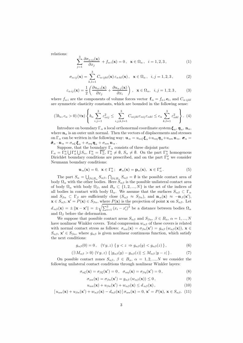
3 Variational formulations

For each body Ωα consider Sobolev space Vα = [H1(Ωα)]3 and the closed sub-

space V 0α = uα ∈ Vα : uα = 0 on Γu

α. All values of the elements from thesespaces on the parts of boundary Γα should be understood as traces. The traceof element uα ∈ Vα on the part Γu

α should belong to space [H1/2(Γuα)]

3, andthe trace of element from V 0

α on the part Ξα = int (Γα \ Γuα) should belong to

[H1/200 (Ξα)]

3.

Define Hilbert space V0 =∏N

α=1Vα with scalar product

(u ,v)V0=

∑Nα=1

(uα,vα)Vαand norm ‖u‖V0

= (u ,u)1/2V0

, u,v ∈ V0. Moreover,

introduce following spaces W =∏

α, β∈QH1/200 (Ξα) = w = (wαβ)

⊤α, β∈Q :

wαβ ∈ H1/200 and U0 = V0 ×W = U = (u,w)⊤ : u ∈ V0, w ∈ W, where

Q = α, β : α ∈ 1, 2, ..., N , β ∈ Bα.In space U0 consider the closed convex set of all displacements, which satisfy

nonpenentration contact conditions:

K = U ∈ U0 : uαn + uβn + wαβ ≤ dαβ on Sαβ , α, β ∈ Q , (12)

where uαn = nα · uα ∈ H1/200 (Ξα), wαβ , dαβ ∈ H

1/200 (Ξα).

Let us introduce bilinear form A(u,v), such that A(u,u) represents thetotal elastic deformation energy of the bodies, linear form L(u), which is equalto external forces work, and nonquadratic functional H(w), which representsthe total deformation energy of nonlinear Winkler layers:

A (u,v) =N∑

α=1

aα(uα,vα), aα(uα,vα) =

∫

Ωα

σσσα(uα) : εεεα(vα) dΩ , (13)

L (u) =

N∑

α=1

lα(uα), lα(uα) =

∫

Ωα

fα · uα dΩ +

∫

Γσα

pα · uα dS , (14)

H(w) =∑

α, β∈Q

∫

Sαβ

[∫ wαβ

0

gαβ(z) dz

]

dS , u,v ∈ V0 , w ∈ W , (15)

where fα ∈ [L2(Ωα)]3, pα ∈ [H

−1/200 (Ξα)]

3, α = 1, 2, ..., N .We have shown, that if condition (4) holds then bilinear form A is sym-

metric, continuous and coercive, and nonquadratic functional H is Gateauxdifferentiable:

H ′(w, z) =∑

α, β∈Q

∫

Sαβ

gαβ(wαβ) zαβ dS , w, z ∈W . (16)

Theorem 1. Suppose that conditions (4), (6), (7) hold. Then problem (1)–(3), (5), (8)–(11) has an alternative weak formulation as the following mini-mization problem:

F (U) = A (u,u)/2− L (u) +H(w) → minU∈K

. (17)

Moreover, there exists a unique solution of problem (17), and this problem isequivalent to the following nonlinear variational inequality on set K:

F ′(U,V −U) = A (u,v − u)− L (v− u) +H ′(w, z−w) ≥ 0 , ∀ (v, z)⊤ ∈ K .(18)

4

Except this variational formulation, we also have proposed another weakformulation of original contact problem in the form of nonlinear variationalequation.

Let us introduce the following nonquadratic functional in space V0:

J(u) =∑

α, β∈Q

∫

Sαβ

[

∫ dαβ−uαn−uβn

0

g−αβ(z) dz

]

dS , u ∈ V0 , (19)

where g−αβ(z) = 0 , z ≥ 0 ∨ gαβ(z) , z < 0 is nonlinear function.Functional J(u) is nonnegative and Gateaux differentiable in V0:

J ′(u,v) = −∑

α, β∈Q

∫

Sαβ

g−αβ(dαβ − uαn − uβn) [vαn + vβn] dS . (20)

We have shown that if conditions (6) and (7) hold, then Gateaux differentialJ ′(u,v) satisfies the following properties:

(∀u ∈ V0) (∃ R > 0 ) (∀v ∈ V0)

|J ′(u,v)| ≤ R ‖v‖V0

, (21)

(∃ D > 0) (∀u,v,w∈V0)

|J ′(u+w,v)−J ′(u,v)|≤D ‖v‖V0‖w‖V0

, (22)

(∀u,v ∈ V0) J′(u+ v,v) − J ′(u,v) ≥ 0 . (23)

These properties helped us to prove the next theorem.Theorem 2. Suppose that conditions (4), (6) and (7) hold. Then the

contact problem (1)–(3), (5), (8)–(11) is equivalent to problem (1)–(3), (5), (8)with the following nonlinear boundary value conditions on the possible contactareas:

σαn(x) = σβn(x′) = g−αβ (dαβ(x)− uαn(x) − uβn(x

′)) , x′ = P (x) , x ∈ Sαβ ,(24)

and it is equivalent in weak sense to the next nonquadratic minimization prob-lem:

F1(u) = A (u,u)/2− L (u) + J(u) → minu∈V0

. (25)

Moreover, problem (25) has a unique solution and is equivalent to the nextnonlinear variational equation in space V0:

F ′1(u,v) = A (u,v) + J ′(u,v) − L (v) = 0, ∀v ∈ V0 , u ∈ V0 . (26)

4 Nonstationary iterative methods

In reflexive Banach space V consider an abstract nonlinear variational equation

Φ (u,v) = Y (v) , ∀v ∈ V, u ∈ V, (27)

where Φ : V × V → R is a functional, which is linear in v, but nonlinear inu, and Y : V → R is linear continuous form. For numerical solution of (27)consider the next nonstationary iterative method [5, 11]:

Gk(uk+1,v) = Gk(uk,v) − γk[

Φ (uk,v) − Y (v)]

, k = 0, 1, ... , (28)

5

where Gk : V × V → R are some given bilinear forms, γk ∈ R are iterativeparameters, and uk ∈ V is the k -th approximation to the exact solution ofproblem (27).

Theorem 3. [5] Suppose that functional Φ satisfies the following properties:

(∀u ∈ V ) (∃RΦ > 0 ) (∀v ∈ V ) |Φ (u,v)| ≤ RΦ ‖v‖V , (29)

(∃DΦ>0) (∀u,v,w∈V ) |Φ (u+w,v) − Φ (u,v)| ≤ DΦ‖v‖V ‖w‖V , (30)

(∃BΦ > 0) (∀u,v ∈ V )

Φ (u+ v,v) − Φ (u,v) ≥ BΦ ‖v‖2V

. (31)

Then nonlinear variational equation (27) has a unique solution u ∈ V . Inaddition, suppose that bilinear forms Gk, k = 0, 1, ... are symmetric, continuouswith constant M∗

G > 0, coercive with constant B∗G > 0, and the next conditions

hold:(∃k0 ∈ N0) (∀k ≥ k0) (∀u ∈ V )

Gk(u,u) ≥ Gk+1(u,u)

, (32)(

∃ε ∈ (0, γ∗), γ∗ = BΦB∗G

/

D2Φ

)

(∃k1) (∀k ≥ k1)

γk ∈ [ε, 2γ∗ − ε]

, (33)

where uk ⊂ V is obtained by iterative method (28).

5 Domain decomposition schemes

Now let us apply nonstationary iterative method (28) for solving nonlinear vari-ational equation (26), which corresponds to original contact problem. Thisequation can be written in form (27), where Φ(u,v) = A (u,v) + J ′(u,v) ,Y (v) = L (v) , u,v ∈ V , V = V0 , and iterative method (28) applied to solve(26) rewrites as follows:

Gk(uk+1,v) = Gk(uk,v)−γk[

A (uk,v) + J ′(uk,v) − L(v)]

, k = 0, 1, .... (34)

Note, that in general case iterative method (34) does not lead to domaindecomposition. Let us propose such variants of this method, which involve thedomain decomposition. At first, let us take bilinear forms Gk in method (34)as follows:

Gk(u,v) = ∂2F1(uk,u,v) = A (u,v) + ∂2J(uk,u,v) , u,v ∈ V0 , (35)

∂2J(uk,u,v) =∑

α, β∈Q

∫

Sαβ

χkαβ g

′αβ(dαβ−u

kαn−u

kβn) [uαn + uβn] [vαn + vβn] dS,

χkαβ = −[ sgn (dαβ−u

kαn−u

kβn) ]

− = 0, dαβ−ukαn−u

kβn ≥ 0 ∨ 1, else . (36)

Here ∂2F1(uk,u,v) and ∂2J(uk,u,v) are the second subdifferentials of func-

tionals F1 and J in point uk ∈ V0. In the case when γk = 1, k = 0, 1, ... ,iterative method (34) with bilinear forms (35) corresponds to semismooth New-ton method for variational equation (26). However, this method does not leadto domain decomposition.

Now, let us take bilinear forms Gk in the following way:

Gk(u,v) = A (u,v) +Xk(u,v) , u,v ∈ V0 , (37)

6

Xk(u,v) =

N∑

α=1

∑

β∈Bα

∫

Sαβ

ψkαβ g

′αβ(dαβ−u

kαn−u

kβn)uαnvαndS, u,v ∈ V0, (38)

where ψkαβ(x) = 1, x ∈ Sk

αβ ∨ 0, x ∈ Sαβ\Skαβ are characteristic functions

of some given subsets Skαβ ⊆ Sαβ of possible contact areas.

Let us show, that such choice of bilinear forms Gk involves the domaindecomposition. Introduce a notation uk+1 = (uk+1 − uk)/γk + uk ∈ V0. Theniterative method (34) with bilinear forms (37) can be written in such way:

A (uk+1,v) +Xk(uk+1,v) = L (v) +Xk(uk,v)− J ′(uk,v) , ∀v ∈ V0 . (39)

uk+1 = γk uk+1 + (1− γk)uk, k = 0, 1, ... . (40)

Since the common quantities of the subdomains are known from the pre-vious iteration, variational equation (39) splits into N separate equations insubdomains Ωα , and iterative method (39)–(40) can be written in the followingequivalent form:

aα(uk+1α ,vα) +

∑

β ∈Bα

∫

Sαβ

ψkαβ g

′αβ(dαβ − ukαn − ukβn) u

k+1αn vαn dS =

= lα(vα) +∑

β ∈Bα

∫

Sαβ

ψkαβ g

′αβ(dαβ − ukαn − ukβn)u

kαnvαn dS+

+∑

β ∈Bα

∫

Sαβ

g−αβ(dαβ − ukαn − ukβn) vαn dS , ∀vα ∈ V 0α , (41)

uk+1α = γk uk+1

α + (1 − γk)ukα , α = 1, 2, ..., N, k = 0, 1, ... . (42)

In each iteration k of method (41)–(42), we have to solve N linear varia-tional equations (41) in parallel, which correspond to linear elasticity problemsin separate bodies Ωα with Robin boundary conditions on possible contact areas.Therefore, this method refers to parallel Robin–Robin type domain decomposi-tion schemes.

By taking different characteristic functions ψkαβ , we can obtain different

particular cases of domain decomposition method (41)–(42). Thus, takingψkαβ(x) ≡ 0 (Sk

αβ = ∅), ∀α, β, ∀k, we get parallel Neumann–Neumann domain

decomposition scheme. Other borderline case is when ψkαβ(x) ≡ 1 (Sk

αβ = Sαβ),∀α, β, ∀k.

Moreover, we can choose characteristic functions ψkαβ by formula (36), i.e.

ψkαβ = χk

αβ . Numerical experiments, provided by us, have shown, that suchDDM has higher convergence rate than other particular domain decompositionschemes.

6 Numerical investigations

Numerical investigations of proposed DDMs have been made for plane problemof unilateral contact between two isotropic bodies Ω1 and Ω2, one of which hasa groove (Fig. 1b). The bodies are uniformly loaded by normal stress withintencity q = 10MPa. Each body has length l = 4 cm and height h = 1 cm.

7

The Young’s moduli and Poisson’s ratios of the bodies are the same: E1 =E2 = 2.1 · 105MPa, ν1 = ν2 = 0.3. The distance between bodies is d12(x) =

r

[ 1− (x1 − l)2/

b2]+3/2

, x ∈ S12 , where b = 1 cm, r = 5 · 10−4 cm, z+ =

max 0, z, S12 =

x = (x1, x2)⊤ : x1 ∈ [0, l], x2 = h

.Across possible contact area S12 there is a nonlinear Winkler layer. The

relationship between normal contact stresses and displacements of this layer aredescribed by the following power function:

g12 (w12(x)) = B−1/a sgn (w12(x)) |w12(x)|1/a

, x ∈ S12 , where parameters Band a are taken from the intervals B ∈ [ 10−6 cm/(MPa)a, 2 ·10−4 cm/(MPa)a ] ,a ∈ [ 0.1, 1 ]. For such choice of these parameters the nonlinear Winkler layermodels a roughness of the possible contact surface [6].

This problem has been solved by DDM (41)–(42) with stationary iterativeparameters γk = γ, ∀ k and characteristic functions ψk

12, taken by formula (36),i.e. ψk

12 = χk12, ∀ k. For solving linear variational problems (41) in each iteration

k we have used finite element method with 8192 linear triangular elements foreach body.

We have used the following initial guesses for displacements u01n(x) ≡ 10−4,u02n(x) ≡ 10−4 and the next stopping criterion: ρk+1

α =∥

∥uk+1αn − ukαn

∥

∥

2/

∥

∥uk+1αn

∥

∥

2≤ εu, α = 1, 2, where ‖uαn‖2 =

√

∑

j [uαn(xj)]2is discrete norm,

xj ∈ S12 are finite element nodes on the possible contact area, and εu > 0 isrelative accuracy.

20 40 60 800

0.05

k

r2

k

65

7

1

2

3

4

8 9

1 2 3 4

0

1

4

3

2

1

1

1 2 3 4

x1 [cm]

[MPa]

s1n

-40

-10

-20

a) b)

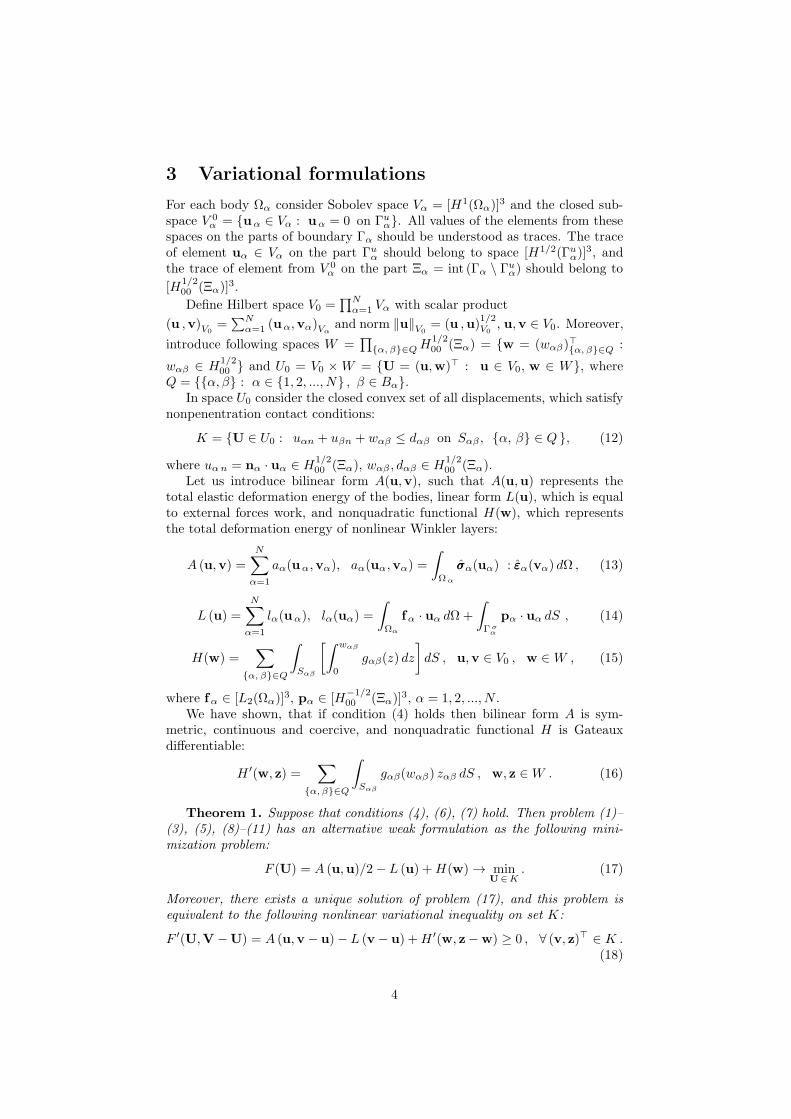
Figure 2: Relative error (a), and normal contact stress (b)

At Fig. 2a the relative error ρk2 of displacement u2n on different iterationsk, obtained for B = 2.5 · 10−5 cm/(MPa)a, a = 0.5, is represented for differentvalues of parameter γ. Curves 1–9 correspond to γ = 0.01, 0.02, 0.05, 0.6, 0.8(0.3), 0.9, 0.95, 0.98, 0.99. For these values of parameter γ, DDM (41)–(42)reaches the accuracy εu = 10−3 in 193, 124, 65, 7, 13, 27, 55, 134 iterationsrespectively.

Thus, we conclude, that the best convergence rate reaches if γ = 0.6. Theconvergence rate is good if γ ∈ [ 0.1, 0.9 ]. However, it becomes slow when γis close to 0 or to 1. For γ = 0.98 the method is still convergent, but theconvergence becomes nonmonotone. For γ ≥ 0.99 the method is not anymoreconvergent.

At Fig. 2b the normal contact stress σ1n = σ2n, obtained by DDM (41)–(42)for B = 10−5 cm/(MPa)a and different values of parameters a is represented.

8

Curves 1–4 correspond to numerical solution for a = 0.3, 0.6, 0.8, 1. Dashedcurve represents the analytical solution, obtained in [13] for contact of twohalfspaces without nonlinear layer. Here we conclude, that for small values of a(a ≤ 0.3) the influence of nonlinear layer on the contact behavior is not so largeand the numerical solutions are close to the solution without layer. However,for larger values of a (a ≥ 0.5) the influence of nonlinear layer becomes moresignificant and can not be neglected.

The positive feature of proposed domain decomposition methods are thesimplicity of their algorithms. These methods have only one iteration loop,which deals with domain decomposition, nonlinearity of Winkler layers andcontact conditions.

References

[1] Bayada, G., Sabil, J., Sassi, T.: A Neumann–Neumann domain decompo-sition algorithm for the Signorini problem. Applied Mathematics Letters17(10), 1153–1159 (2004)

[2] Bresch, D., Koko, J.: An optimization-based domain decompositionmethod for nonlinear wall laws in coupled systems. Math. Models MethodsAppl. Sci. 14(7), 1085–1101 (2004)

[3] Dostal, Z., Kozubek, T., Vondrak, V., Brzobohaty, T., Markopoulos, A.:Scalable TFETI algorithm for the solution of multibody contact problemsof elasticity. Int. J. Numer. Methods Engrg. 41, 675–696 (2010)

[4] Dyyak, I.I., Prokopyshyn, I.I.: Domain decomposition schemes for friction-less multibody contact problems of elasticity. In: G.K. et al. (ed.) Numer-ical Mathematics and Advanced Applications 2009, pp. 297–305. Springer(2010)

[5] Dyyak, I.I., Prokopyshyn, I.I., Prokopyshyn, I.A.: Penalty Robin–Robin domain decomposition methods for unilateral multibody con-tact problems of elasticity: Convergence results (2012). URLhttp://arxiv.org/pdf/1208.6478.pdf

[6] Goryacheva, I.G.: Contact mechanics in tribology. Kluwer (1998)

[7] Hintermuller, M., Ito, K., Kunisch, K.: The primal-dual active set strategyas semismooth Newton method. SIAM J. OPTIM. 13(3), 865–888 (2003)

[8] Koko, J.: Convergence analysis of optimization-based domain decompo-sition methods for a bonded structure. Applied Numerical Mathematics(58), 69–87 (2008)

[9] Koko, J.: Uzawa block relaxation domain decomposition method for atwo-body frictionless contact problem. Applied Mathematics Letters 22,1534–1538 (2009)

[10] Prokopyshyn, I.I.: Parallel domain decomposition schemes for frictionlesscontact problems of elasticity. Visnyk Lviv Univ. Ser. Appl. Math. Comp.Sci. 14, 123–133 (2008). [In Ukrainian]

9

[11] Prokopyshyn, I.I., Dyyak, I.I., Martynyak, R.M., Prokopy-shyn, I.A.: Penalty Robin–Robin domain decomposition schemesfor contact problems of nonlinear elastic bodies (2012). URLhttp://arxiv.org/pdf/1209.1129.pdf. [Accepted to DD20 Pro-ceedings]

[12] Sassi, T., Ipopa, M., Roux, F.X.: Generalization of Lion’s nonoverlappingdomain decomposition method for contact problems. Lect. Notes Comput.Sci. Eng. 60, 623–630 (2008)

[13] Shvets, R.M., Martynyak, R.M., Kryshtafovych, A.A.: Discontinuous con-tact of an anisotropic half-plane and a rigid base with disturbed surface.Int. J. Engng. Sci. 34(2), 183–200 (1996)

[14] Suquet, P.M.: Discontinuities and plasticity. In: CISM Courses Lect., 302,pp. 279–340 (1988)

[15] Vorovich, I.I., Alexandrov, V.M. (eds.): Contact Mechanics. Fizmatlit,Moscow (2001)

[16] Wohlmuth, B.: Variationally consistent discretization schemes and numer-ical algorithms for contact problems. Acta Numerica 20, 569–734 (2011)

10