arX

iv:1

104.

3516

v1 [

cond

-mat

.sof

t] 1

8 A

pr 2

011

An Adaptive Hierarchical Domain Decomposition Method for Parallel

Contact Dynamics Simulations of Granular Materials

Zahra Shojaaee∗, M. Reza Shaebani, Lothar Brendel, Janos Torok, Dietrich E. Wolf

Computational and Statistical Physics Group, Department of Theoretical Physics, University of Duisburg-Essen, 47048

Duisburg, Germany

Abstract

A fully parallel version of the Contact dynamics (CD) method is presented in this paper. For large enoughsystems, 100% efficiency is reached for an arbitrary number of processors using hierarchical domain de-composition with dynamical load balancing. The iterative scheme to calculate the contact forces is leftdomain-wise sequential, with data exchange after each iteration step, which ensures its stability. Additionaliterations due to partially parallel update at the domain boundaries vanish with increasing number of par-ticles, which allows for an effective parallelization. We found no significant influence of the parallelizationon the physical properties.

Keywords: Contact dynamics method, Granular materials, Hierarchical domain decomposition, Loadbalancing, MPI libraryPACS: 45.70.-n, 02.70.-c, 45.10.-b

1. Introduction

Discrete element method simulations have been widely employed in scientific studies and industrial ap-plications to understand the behavior of complex many-particle systems such as granular materials. Thecommon property of these methods is that the time evolution of the system is treated on the level of in-dividual particles, i.e. the trajectory of each particle is calculated by integrating its equations of motion.Among the discrete element methods, soft particle molecular dynamics (MD) [1, 2], event driven (ED) [3, 4]and contact dynamics (CD) [5, 6, 7, 8] are often used for simulating granular media.

Molecular dynamics is the most widely used algorithm for discrete element simulations. For granularmaterials, the contact forces between the soft particles stem from visco-elastic force laws. Interactionsare local, therefore efficient parallelization is possible [9, 10, 11, 12] with 100% efficiency for large systems(Throughout the paper, the performance of a parallel algorithm is quantified by the usual quantities: thespeed-up S(Np), which is the ratio of the run time of the non-parallel version on a single processor to the runtime of the parallel version on Np processors, and the efficiency E=S/Np). The time step and therefore thespeed of MD simulations is strongly limited by the stiffness of the particles, as collisions must be sufficientlyresolved in time. This makes molecular dynamics efficient for dense systems of soft particles, but it breaksdown in efficiency in the hard particle and dilute system limit.

The Event driven dynamics [13, 14] considers particle interaction to be negligible in duration comparedto the time between collisions. Particle collisions are thus treated as instantaneous events and trajectoriesare analytically integrated in between. This makes ED favorable in dilute granular systems, where the abovecondition holds. The parallelization of this algorithm poses extreme difficulties, since the collisional eventsare taken from a global list, which in turn is changed by the actual collision. In general, a naive domain

∗Corresponding authorEmail address: zahra.shojaaee@uni-duisburg-essen.de (Zahra Shojaaee)

Preprint submitted to Journal of Computational Physics April 19, 2011

decomposition leads to causality problems. The algorithm presented in [15] conserves causality by revertingto an older state when violated. The best efficiency reached so far is a speed up proportional to the squareroot of the number of processors [15].

Contact dynamics works on a different concept to achieve the hard sphere limit: The contact forces arecalculated to fulfill constraints of particle impenetrability and friction laws [8]. For a cluster of touchingparticles, this implicit calculation can only be achieved by a global iteration. On the other hand, thepermitted time steps are much larger than in molecular dynamics [8].

Providing a parallel CD code is motivated by the need for large-scale simulations of dense granular sys-tems of hard particles. The computation time even scales as O(N1+2/d) with the number of particles in CD[8] (d is the dimension of the system), while it grows linearly with N in MD. However, parallelization of CDposes difficulties as in general the most time consuming part of the algorithm is a global iteration proce-dure, which cannot be performed completely in parallel. So far, a static geometrical domain decompositionmethod has been proposed in Ref. [16], and a partially parallel version is introduced in Ref. [17], where onlythe iterative solver is distributed between shared memory CPUs. In the former work, the force calculationis studied just on 8 processors and in the latter, already with 16 processors the performance efficiency isbelow 70%. None of these studies deal with computational load balancing during the execution of the code.

There is a large variety of domain decomposition methods proposed for parallel particle simulationsin the literature, from Voronoi tessellation [18] to orthogonal recursive bisection (ORB) [19, 20]. For theparallelization of CD the size of the interfaces between domains is more crucial than for MD, since besidescommunication overhead it also influences the parallel/sequential nature of the global iteration. So the ORBmethods are the most suited for the CD code together with adaptive load balancing approaches [21], whichis not only important in heterogeneous clusters but also in the case of changing simulation setup and localparticle/contact density.

In the present work, we introduce a completely parallel version of the contact dynamics method usingMPI communication with orthogonal recursive bisection domain decomposition for an arbitrary number ofprocessors. The method minimizes the computational costs by optimizing the surface-to-volume ratio ofthe subdomains, and it is coupled with an adaptive load balancing procedure. The validation of our code isdone by numerical simulations of different test systems.

This article is organized as follows. The contact dynamics method is described briefly in Sec. 2 andparticular attention is paid to the numerical stability of the sequential and parallel update schemes, and tothe identification of the most time consuming parts of the code. In Sec. 3 we present an adaptive domaindecomposition method, and implement it in a parallel version of the CD algorithm. The results of some testsimulations with respect to the performance of the parallel CD code are presented in Sec. 4 and the effectof our parallelization approach on the physical properties of the solutions are investigated. We conclude thepaper in Sec. 5 with a summary of the work and a brief discussion.

2. Contact Dynamics Method

2.1. A brief description of the CD algorithm

In this section, we present the basic principles of the CD method, with special emphasis on thoseparts where changes are applied in the parallel version of the code. A more detailed description of thissimulation method can be found in [8]. Contact dynamics is a discrete element method, where the equationsof motion describe the movement of the particles. However, the forces are not calculated from particledeformation, instead they are obtained from the constraints of impenetrability and friction laws. Imposingconstraints requires implicit forces, which are calculated to counteract all movement that would causeconstraint violation.

In general for molecular dynamics, where trajectories are smooth (soft particle model), simulation codesuse second (or higher) order schemes to integrate the particle positions. In CD method, the non-smoothmechanics (hard particle limit) requires strong discontinuity, which can only be achieved by first orderschemes. Thus we apply an implicit first-order Euler scheme for the time stepping of particle i:

~vi(t+∆t) = ~vi(t) +1

mi

~Fi(t+∆t)∆t, (1)

2

~ri(t+∆t) = ~ri(t) + ~vi(t+∆t)∆t , (2)

which determines the new velocity ~vi and position ~ri of the center of mass of the particle after a time step∆t. The effective force on particle i is denoted by Fi. The size of the time step ∆t is chosen such thatthe relative displacement of the neighboring particles during one time step is much smaller compared to thesize of particles and to the radius of curvature of contacting surfaces. Similar equations are used for therotational degrees of freedom, i.e. to obtain the new angular velocity ~ωi(t+∆t) (caused by the new torque~Ti(t+∆t)), and the new orientation of particle i.

For simplicity, in the following we assume that particles are dry and non-cohesive having only unilateralrepulsive contact forces. Furthermore, we assume perfectly inelastic particles, which remain in contact aftercollision and do not rebounce. The implicit scheme must fulfill the following two constraints:

(i) the impenetrability condition: the overlapping of two adjacent particles has to be prevented by thecontact force between them.

(ii) the no-slip condition: the contact force has to keep the contact from sliding below the Coulomb frictionlimit, i.e. the tangential component of the contact force cannot be larger than the friction coefficienttimes the normal force.

The contact forces should be calculated in such a way that the constraint conditions are satisfied at timet+∆t, for the new particle configuration [8]. Once the total force and torque acting on the particles, includingthe external forces and also the contact forces from the adjacent particles, are determined, one can let thesystem evolve from time t to t+∆t.

Let us now consider a pair of neighboring rigid particles in contact or with a small gap between them asshown in Fig. 1. We define ~n as the unit vector along the shortest path of length g between the surfaces ofthe two particles. The relative velocity of the closest points is called the relative velocity of the contact ~vg.In the case that the particles are in contact, the gap g equals to zero, and ~n denotes the contact normal.

We first assume that there will be no interaction between the two particles at t+∆t, i.e. the new contactforce ~R(t+∆t) equals to zero. This allows the calculation of a hypothetical new relative velocity of the twoparticles ~vg,0(t+∆t) through Eq. (1), only affected by the remaining forces on the two particles. The newgap reads as:

g(t+∆t) = g(t) + ~vg,0(t+∆t)·~n∆t. (3)

If the new gap stays indeed positive (0<g(t+∆t)) then no contact is formed and the zero contact force is

kept: ~R(t+∆t)=0.On the other hand, if the gap turns out to be negative (g(t+∆t) ≤ 0), a finite contact force must be

applied. First, we determine the new relative velocity from the condition that the particles remain in contactafter the collision,

0 ≡ g(t+∆t)~n = g(t)~n+ ~vg(t+∆t)∆t (4)

Here we assume sticking contacts with no relative velocity in the tangential direction (~v tg (t+∆t)=0), which

implies that the Coulomb condition holds. The new contact force satisfying the impenetrability can be

Figure 1: Schematic picture showing two adjacent rigid particles.

3

obtained using Eq. (1) as

~R(t+∆t) =M

∆t

(

~vg(t+∆t)− ~vg,0(t+∆t)

)

=−M

∆t

(

g(t)

∆t~n+ ~vg,0(t+∆t)

)

(5)

where the mass matrix M, which is built up from the masses and moments of inertia of both particles [8],

reflects the inertia of the contact so that M−1 ~R corresponds to the relative acceleration of the contactingsurfaces induced by the contact force ~R.

At this point, we have to check for the second constraint: the Coulomb friction. Let us first define thenormal and tangential contact forces:

Rn(t) ≡ ~R(t)·~n ,~Rt(t) ≡ ~R(t)−Rn(t)~n . (6)

Then the Coulomb inequality reads as∣

∣

∣

~Rt(t+∆t)∣

∣

∣≤ µRn(t+∆t) , (7)

with µ being the friction coefficient. If the inequality (7) holds true, then we have already got the correctcontact forces. Otherwise, the contact is sliding, i.e. ~vg(t+∆t) has a tangential component and Eq. (4) reads

0 ≡ g(t+∆t) = g(t) + ~n·~vg(t+∆t)∆t , (8)

which determines the normal component of ~vg(t+∆t). The remaining five unknowns, three components of

the contact force ~R(t+∆t) and two tangential components of the relative velocity, are determined by thefollowing two equations:

(i) Impenetrability by combining Eqs. (4) and (5)

~R(t+∆t)=M

∆t

(

−g(t)

∆t~n+ ~v t

g (t+∆t)− ~vg,0(t+∆t)

)

. (9)

(ii) Coulomb condition

~Rt(t+∆t) = −µRn(t+∆t)~v tg (t+∆t)

∣

∣~v tg (t+∆t)

∣

∣

. (10)

Figure 2 summarizes the force calculation process for a single incipient or existing contact. Assumingthat all other forces acting on the participating particles are known, the Nassi-Shneiderman diagram inFig. 2 enables us to determine the contact force.

❍❍❍❍❍❍❍❍

✭✭✭✭✭✭✭✭✭✭✭✭✭✭✭✭✭✭✭✭✭✭✭✭

g(t)+~vg,0(t+∆t)·~n∆t > 0Yes No~R(t + ∆t)=0

No Conta tEvaluation of ~Rtest via Eq. (5)

PPPPPPPPP

✥✥✥✥✥✥✥✥✥✥✥✥✥✥✥

∣

∣

∣

~Rt test∣∣∣ ≤ µRtestnYes No~R(t+∆t)= ~RtestSti king Conta t Evaluation of ~R(t + ∆t) viaEqs. (9) and (10)Sliding Conta t

1

Figure 2: The force calculation process for a single contact.

4

Figure 3: The diagram of the main steps of the contact dynamics algorithm.

The above process assumes that apart from the contact forces all other interactions are known for theselected two particles. However, in dense granular media, many particles interact simultaneously and forma contact network, which may even span the whole system. In such cases, the contact forces cannot bedetermined locally because each unknown contact force depends on the adjacent unknown contact forcesacting on the particles. In order to find the unilateral frictional forces throughout the entire contact network,an iterative method is mostly used in CD as follows: At each iteration step, we choose the contacts randomlyone by one and calculate the new contact force considering the surrounding contact forces to be already thecorrect ones. It is natural to update the contact forces sequentially in the sense that each freshly calculatedforce is immediately used for further force calculations. One iteration step does not provide a globallyconsistent solution, but slightly approaches it. Therefore, the iteration has to be repeated many times untilthe forces relax towards an admissible state.

The precision of the solution increases smoothly with the number of iterations NI , with the exact solutionbeing only reached for NI → ∞. Of course we stop at finite NI . It is optional to use a fixed number ofiterations at each time step, or to prescribe a given precision to the contact force convergence and let NI tovary at each time step.

Breaking the iteration loop after finite iteration steps is an inevitable source of numerical error in contactdynamics simulations, which mainly results in overlap of the particles and in spurious elastic behavior [22].Occurring oscillations are a sign that the iterations were not run long enough to allow the force informationappearing on one side of the system to reach the other side. This effect should be avoided and the numberof iterations should be chosen correspondingly [22].

Once the iteration is stopped, one has to update the particle positions based on the freshly calculatedforces acting on the particles. Figure 3 concludes this section with a diagram depicting the basic steps ofthe contact dynamics algorithm.

2.2. CPU time analysis

The CD algorithm described in the previous section has three main parts: (i) The contact detection, (ii)the force calculation (iteration), (iii) the time evolution. In this section we analyze the CPU consumptionof all these parts.

Given a system and the contact detection algorithm, the time consumption of parts (i) and (iii) can beeasily estimated. On the other hand, the computational resource needed by part (ii) is strongly influencedby the number of iterations. If one uses extremely high values of NI , part (ii) will dominate the CPU usage.This led Renouf et al. [17] to the conclusion that parallelizing the force calculation is enough.

Our view is that the situation is more delicate and it is demonstrated by a simulation in which dilutedgranular material is compressed until a dense packing is reached [23]. The system consists of 1000 polydis-perse disks in two dimensions with friction coefficient µ=0.5. The stopping criteria for the iteration was thefulfillment of any of the two conditions:

(1) The change in the relative average force is less than 10−6.

5

Figure 4: (color online) The percentage of CPU time consumption as a function of time. The insets show typical configurationsof particles at different packing fractions. The thickness of the inter-center connecting red lines is proportional to the magnitudeof the contact force.

(2) NI ≥ 200

Figure 4 shows the evolution of the relative CPU time consumption of the different parts of the algorithm.The time stepping contribution always remains less than 5%, and the rest is divided between the other twosubroutines. Initially, the contact detection task consumes the majority of the computational time. Aftera while, clusters of contacting particles form, and the cost of force calculation increases and the iterativesolver gradually becomes the most time consuming part of the code. Note that the contribution of the solversaturates to 70% of the total elapsed time. If only the force calculation part is executed in parallel, evenwith Eforce = 100%, the remaining 30% non-parallel portions set an upper limit to the overall efficiency Eand the speed-up S of the code (Emax ≈ 80% and Smax ≈ 4). Therefore, we aim to provide a fully parallelversion of CD which operates efficiently in all density regimes.

2.3. Sequential versus parallel update scheme

As we pointed out in Sec. 2.1, the problem of finding the unilateral frictional contact forces that satisfythe constraint conditions cannot be solved locally in a dense granular system. In order to evaluate thenew value of a single contact, one has to know the new values of the adjacent contact forces, which areunknown as well, i.e. all contact forces are coupled in a cluster of contacting particles. Note that this is aconsequence of the infinite stiffness of the particles; a single collision influences the entire network of contactforces between perfectly rigid particles. This problem is solved by iterating through all contacts many timesuntil a given precision is reached.

Similarly to solving the Laplace equation, the information about a disturbance (e.g. collision of a newparticle) appearing on one side of a cluster must diffuse through the whole cluster to satisfy the constraints.Actually, the iteration scheme is very similar to two traditional schemes for solving a set of linear equations[24], albeit with nonlinearities introduced by the change of contact states (repulsive vs. force-less, sticking vs.sliding): the Jacobi scheme and the Gauss-Seidel scheme, corresponding to parallel and sequential contactupdating, respectively.

Here we denote (i) sequential, where the contacts are solved one by one using always the newest informa-tion available, which is a mixture of new and old values, (ii) parallel, where all contacts are updated usingthe old values, and substituted with the new ones at the end of the iteration step. Needless to say that thesecond case is favored for parallel applications but instabilities may appear (like when combining the Jacobischeme with Successive Over-Relaxation [24]). To study its impact, we investigated a mixed method, where

6

0 200 400 600 800 1000 1200 1400 1600N

I

10-3

10-2

10-1

100

101

a mea

n/aex

t

p=0.00p=0.55p=0.65p=0.67p=0.68p=0.69p=0.70p=0.71

Figure 5: (color online) The mean acceleration of the particles amean scaled by aext=2rPext/m (where r and m are the meanparticle radius and mass, respectively, and Pext is the external pressure) in terms of the number of iterations NI for severalvalues of the “parallelness” p (cf. text).

a fraction p of the contacts are updated in parallel and the rest sequentially. First, a static homogeneouspacking is generated by applying an external confining pressure [23]. Next, the inter-particle forces are setto zero, while the positions of the particles and the boundary conditions are kept fixed. Now the coderecalculates the contact forces within one time step with an unconstrained number of iterations until theconvergence is reached. We check how many iteration steps are needed to find a consistent equilibriumsolution with a given accuracy threshold. The results are shown in Fig. 5.

It turns out that, on average, the number of iterations NI to reach a given accuracy level increases withincreasing p. For high values of p, fluctuations appear and beyond pc ≈ 0.65 the iterative solver is practicallyunable to find a consistent solution. The critical ratio pc depends slightly on the simulation conditions. Wediscuss the consequence of this behavior for the parallel version of CD in Secs. 3 and 4.

Thus, the results of our numerical simulations reveal that the sequential update scheme is quite robustand the force convergence is reached smoothly, while the fully parallel update scheme is highly unstable.However, there is a limit of parallel update for which the iteration remains stable. This is important becausethe domain decomposition method allows for a sequential update only in the bulk of each domain, whilethe boundary contacts are updated in a parallel way (cf. section 3.1). This analysis suggests that the ratioof bulk contacts to boundary ones after the decomposition should never fall below 1. Fortunately, this isassured in a domain decomposition context anyway.

3. A parallel version of the CD algorithm

3.1. The parallel algorithm

A parallel version of the CD algorithm based on the decomposition of the simulation domain is introducedin this section. The main challenge is to properly evaluate the inter-particle forces when the contact networkis broken into several subnetworks assigned to different processors. The parallelization presented in thissection is valid only for spherical particles (disks in 2D), but it is straightforward to extend it for othershape types.

At the beginning of the simulation, a domain decomposition function is called to divide the systembetween Np processors. Regarding the fact that neither the performance of the computing environment nor

7

Figure 6: (color online) Schematic picture showing two neighboring processors at their common interface. Their respectivedomain and boundary regions are marked. Particle A is a native particle of processor 1 and is in contact (asterisks) with twoforeign particles, namely boundary particles of processor 2. The contacts are boundary contacts of processor 2 and thus foreign

ones to processor 1. Particle B is a boundary particle of processor 2 and has two contacts (asterisks) located inside the domainof processor 1, i.e. they belong to the latter’s boundary contacts.

the density distribution and the internal dynamics of the system are known initially, a uniform distributionfor all relevant factors is assumed and initially the simulation domain is geometrically divided into Np partswith the same volume. The details of the hierarchical decomposition method are explained in Sec. 3.2.

After establishing the domains, the particles are distributed among the processors. Each processormaintains its set of native particles, the center of mass of which lie within its domain. The next task is toidentify in each domain the boundary particles, i.e. those particles which may be in contact with particlesin other domains, as this information should be passed to the neighbors. Two particles may come intocontact if the gap is smaller than 2vmax∆t, where vmax is the maximum velocity in the whole system. Sothe maximal distance between the centers of mass of two particles, which may come into contact is

d ≤ 2rmax + 2vmax∆t, (11)

where rmax is the radius of the largest particles. This distance also defines the width of the boundary region

in which particles may have contact with particles outside a processor’s domain, see also Fig. 6.While rmax is constant during the simulation, vmax varies in time and space. For reasons described

in Sec. 3.2, we use a global upper limit ℓ for the boundary size, which is unchanged during the wholesimulation. It was explained in Sec. 2.1, that the displacement of the particles must be small compared toparticle size for contact dynamics to be valid. Therefore it is legitimate to define the upper limit for theparticle displacement to be 0.1rmax and thus use the boundary size

ℓ = 2.2rmax . (12)

Hence, a small amount of in principle irrelevant neighboring information is transferred. This is dominatedby other effects, though, as will be shown in Sec. 3.2.

After the identification of the boundary particles, their relevant data is sent to the corresponding neighborprocessors, which keep the information of these (to them) foreign particles. Since sender and receiver willalways agree about the forces acting on these particles, the receiver can evolve their state on its own.

The next step is to identify actual and possible contacts between both native and foreign particles. Aposition is assigned to each contact, which is the middle of the gap (see Fig. 1). Obviously, for particlesin touch, this is the contact point. Each processor builds a list of native contacts for the iteration loop

8

Figure 7: (color online) The diagram of the parallel version of CD. The colored regions correspond to the new parts comparedto the original CD algorithm shown in Fig. 3.

exclusively from contacts lying in its domain. The remaining ones are called foreign contacts and are in turnboundary contacts of neighboring processors. During an iteration sweep, they will not be updated but theirforces enter the force calculation algorithm. Only at the end of the sweep, each processor sends the newforces of its boundary contacts to its corresponding neighbor. This means that during an iteration sweep,foreign contacts always have the values from the last iteration, while native contacts are gradually updatedrealizing a mixture of parallel and sequential update.

The convergence of the force calculation has to be checked after each iteration sweep. This should be aglobal test, since the convergence in different subdomains may be achieved at different iteration steps. Thistask can only be completed by a single processor. Therefore, the necessary data is collected and submittedto the root processor, which makes a decision whether the iteration should continue or the convergenceis good enough and time stepping can take place. If further iterations are necessary, then only boundarycontact information are exchanged among neighbors, as particles do not move within the iteration loop.With new foreign contact values, each processor can perform the next iteration sweep. If the iteration loophas finished, the particles are displaced according to the implicit Euler scheme of Eqs. (1) and (2). Everyprocessor is responsible for its own native particles (but evolves its copies of foreign particles as well).

Before starting the next time step, we have to take care of the load balancing: Every processor broadcastsits own elapsed CPU time, which provides the required information to run the load balancing function. Thedetailed description of this function is presented in Sec. 3.3. If the load balancing function redivides thesimulation box, then each processor has to compare its own particle positions to the new domain coordinatesof all other processors to determine to which processor each particle has to be sent. This re-associationof particles takes place also without domain redivision as particles change domains simply due to theirdynamics.

Figure 7 summarizes the parallel algorithm. The main differences (highlighted in the diagram) are that(i) at certain points data must be sent or received to neighboring domains; (ii) the iteration scheme updatesonly native contacts gradually, while foreign contacts are refreshed only after a complete iteration sweep;(iii) load balancing and domain redivision checks take place at the end of the time step.

9

Figure 8: (color online) An initial hierarchical decomposition of the simulation domain for Np = 14.

A mixture of the sequential and the parallel update scheme occurs for a fraction of the contacts. Thisfraction depends on the surface-to-volume ratio of the subdomain. As discussed in Sec. 2.3, a mixed updatecan become unstable if the contribution of the parallel update exceeds a threshold of order unity. Thislimitation coincides with the standard limitation of parallel computation that the boundary region shouldbe negligible compared to the bulk. In this sense, for reasonably large systems, we do not expect anyinstability impact due to the parallel update. Nevertheless, this issue is investigated in Sec. 4.3.

In the next section we introduce a hierarchical domain decomposition method, which finds the best wayto arrange the orientation and location of the interfaces so that the surface-to-volume ratio is minimal fora given number of processors.

3.2. Hierarchical domain decomposition

Before describing the domain decomposition, we have to investigate the contact detection. This process,for which the brute force algorithm scales as O(N2) with the number of particles, can be realized for differentlevels of polydispersity [25, 26, 27] within O(N) CPU cycles. We chose to implement the most widespreadone, the cell method [25], which works well for moderate polydispersity and which is the most suitable forparallel implementation.

The cell method puts a rectangular grid of mesh size ax × ay on the simulation space. Each particle isassigned to its cell according to its position, and the mesh size is chosen such that the particles can only havea contact with particles from neighboring cells and their own. That means, the cell diameter has essentiallythe same meaning as the width of the boundary region ℓ and thus they should coincide. On the other hand,the values ax and ay have to be chosen such that in each direction every domain has an integer number ofcells. But this would mean, in general, a different mesh size for all subdomains, which may be far from theoptimal value. Therefore, it is advantageous (for large systems and moderate polydispersities) to choose aglobal ax and ay instead, and restrict the domain boundaries to this grid.

The domain decomposition method proposed in this paper is based on the orthogonal recursive bisection

algorithm [19] with axis-aligned domain boundaries. The basis of the algorithm is the hierarchical subdivisionof the system. Each division represents recursive halving of domains into two subsequent domains. Theadvantage of such a division is an easy implementation of load balancing, which can be realized at any level,simply by shifting one boundary.

First, we have to group the Np processors (where Np is not required to be a power of two) hierarchicallyinto pairs. The division algorithm we use is the following: We start at level 0 with one node1, which initiallyis a leaf (a node with no children) as well. A new level l is created by branching each node of level l−1in succession into two nodes of level l, creating 2l leaves. This continues until 2l < Np ≤ 2l+1. Then, onlyNp − 2l leaves from level l are branched from left to right, cf. Fig. 8(a).

Next, we have to assign a domain to each leaf/processor. In the beginning, having no information aboutthe system, all domains should have the same size. Actually, their sizes equal only approximatively due togrid restriction described above, cf. Fig. 9(a). To achieve this, the recursive division of the sample is done

1These are abstract nodes in a tree rather than (compounds of) CPUs.

10

according to the tree just described. Each non-leaf node represents a bisection with areas corresponding tothe number of leaves of its branches (subtrees). The direction of the cut is always chosen as to minimize theboundary length.

The hierarchical decomposition method provides the possibility of quick searches through the binarytree structure. For example, the task to find the corresponding subdomain of each particle after loadbalancing requires a search of order O(log(Np)) for Np processors. Further advantages of the hierarchicaldecomposition scheme are that the resolution of the simulation domain can be flexibly adjusted in reactionto the load imbalance between twin processor groups, and local dynamical events only lead to the movementof their interface and higher-level ones, while the lower-level borders are not affected.

3.3. Adaptive load balancing

For homogeneous quasi-static systems, the initially equal-sized subdomains provide already a reasonablyuniform load distribution, but for any other case the domain boundaries should dynamically move duringthe simulation. In the load balancing function, we take advantage of the possibility provided by MPI tomeasure the wall clock time accurately. For every time step, the processors measure the computational timespent on calculations and broadcast it, so that all processors can decide simultaneously whether or not theload balancing procedure has to be executed. To quantify the global load imbalance, the relative standarddeviation of the elapsed CPU time in this time step 2 is calculated via the dimensionless quantity

σT ≡1

〈T 〉

√

〈T 2〉 − 〈T 〉2, (13)

where the average is taken over the processors.A threshold value σ∗

T is defined to control the function of the load balancing algorithm: If σT < σ∗

T , thenthe simulation is continued with the same domain configuration, otherwise load balancing must take place.This load balancing test is performed by all processors simultaneously, since all of them have the necessarydata. The result being the same on all processors, no more communication is needed.

If the above test indicates load imbalance, we have to move the domain boundaries. This may happenat any non-leaf node of the domain hierarchy tree. The relevant parameter for the domain division is thecalculating capacity of the branches, which is defined as

νj =∑

i

Vi

Ti, (14)

where Ti and Vi are the CPU time and volume of domain i, respectively, and the summation includes allleaves under branch j. Let us denote the two branches of a node as j and k, then the domain must bebisectioned according to

νj ≡νj

νj + νkand νk ≡ 1− νj . (15)

The above procedure is repeated for all parent nodes. If the size of a domain was changed, then all subdomainwalls must be recalculated as even with perfect local load balance the orientation of the domain boundarymay be subject to change. Note that boundaries must be aligned to the grid boundaries as explained inSec. 3.2.

As an example, let us consider the situation of Fig. 8 at the node of level 0 with branch 1 to the leftand branch 2 to the right. If all Ti would be the same, then ν1 = 8/14 and ν2 = 6/14, just as the initialconfiguration. Let us now assume that the processors 12 and 13 [top right in Fig. 8(b)] are only half as fastas the others, thus, the elapsed time is twice as much. In this case ν1 = 8/13 and ν2 = 5/13, so the thick,solid division line moves to the right. Furthermore, the thin, solid division line on the right moves up fromthe position 4/6 to 4/5.

2Assuming exclusive access to the computing resources on every processor, we identify wall clock time and CPU timethroughout this work.

11

a)

⇒

CPU

Tim

e

1 2 3 4 5 6 7processor number

b)

⇒

CPU

Tim

e

1 2 3 4 5 6 7processor number

Figure 9: (color online) (a) Geometrical domain decomposition at the beginning of the simulation leads to an unbalanceddistribution of the load over the processors. (b) After load balancing, the volume of the subdomains belonging to differentprocessors vary according to the CPU time it needed in the previous time step and the load distribution over the processorsbecomes more even.

Figure 9 shows how load balancing improves the CPU time distribution over seven processors. Theinitial geometrical decomposition leads to an uneven workload distribution because of the inhomogeneousdensity of the original particle configuration [Fig. 9(a)]. However, the load balancing function manages toapproximately equalize the CPU times in the next time step by moving the borders [Fig. 9(b)].

4. Numerical results

In the following, we present the results of test simulations for different systems performed by the parallelcode. The main question to answer is how efficient is the parallel code, i.e. how much could we speed up thecalculations by means of parallelization. The sensitivity of the performance to the load balancing threshold isalso studied. Finally, the impact of parallelization on the number of iterations and on the physical propertiesof the solutions is investigated.

12

Figure 10: (color online) The simulation setup used for performance tests. The system is confined by two lateral walls in ydirection (exerting a pressure of 0.25 natural units), and periodic boundary conditions are applied in x direction. The packingscontain 500, 8000, and 106 particles with Lx=20, 20, 100 and Ly=20, 320, 10000, respectively. The polydispersity in the smalland medium systems amounts to 20%, while the large system is monodisperse.

4.1. Performance of the force calculation

In this section, we test the efficiency of the parallel algorithm solely with respect to the force calculation.In general, it is the most time consuming part of the contact dynamics simulation (see Sec. 2.2), so theefficient parallelization of the iteration scheme is necessary for the overall performance.

To focus just on the force calculation, we chose test systems where large scale inhomogeneities are absentand adaptive load balancing is unnecessary. Thus, dense static packings of 500, 8000, and 106 particles withperiodic boundary conditions in one direction and confining walls in the other were set up [see Fig. 10]. Thecalculations started with no information about the contact forces and the simulation was stopped when thechange in the relative average force is less than 10−6. Of course, this requires a different number of iterationsdepending on the system size and number of processors.

In order to get rid of perturbing factors like input/output performance, we measured solely the CPUtime spent in the iteration loop. Figure 11 summarizes the test results, which show that if the system is largecompared to the boundary regions, the efficiency is about 100%, which is equivalent to a linear speed-up.The smallest system is inapt for parallelization, as already for only 4 processors the boundary regions takeup 20% of the particles, which induces a large communication overhead. The same fraction of boundaryparticles is reached around Np=32 for the medium sized system with 8000 particles. Therefore, one wouldexpect the same performance for Np=4 and 32 for the small and medium sizes, respectively. In additionto the above mentioned effect, the efficiency of the medium system breaks down at Np=24 due to specialarchitecture of the distributed memory cluster used for simulations (Cray-XT6m with 24 cores per board),since the speed of the inter-board communications is much slower than the intra-board one. The observedefficiency values over 100% are possible through caching, which was already observed in molecular dynamics[12]. The largest system has a large computation task compared to the boundary communication, which ismanifested in almost 100% efficiency. On the other hand, it is also too large for significant caching effectsproducing over 100% efficiency. However, a gradual increase in the efficiency is observed as the domain size(per processor) decreases with increasing the number of processors.

For the medium sized system, we also measured the overall performance including time stepping andload balancing. For this purpose, the top wall was removed and the bottom wall was pushed upwards inorder to generate internal dynamical processes, which unbalances the load distribution. As shown in Fig. 11,

13

a)

1 8 16 24 32 40 48 56 64number of processors

10

20

30

40

50

60

spee

d-up

1 32 64 128 256number of processors

0

50

100

150

200

250

spee

d-up

b)

1 2 4 8 16 32 64 128 25624number of processors

0

50

100

150

200

effi

cien

cy (

%)

500 particles8000 particles8000 particles, overall1,000,000 particles

Figure 11: (color online) (a) Speed-up and (b) efficiency of the force calculations for a small system with 500 particles (fullsquares), a medium system with 8000 particles (full circles), and a large system with 106 particles (full diamonds). The opencircles present the overall efficiency for the medium sized system.

10-4

10-3

10-2

10-1

100

σT

*

20

30

40

50

60

70

80

90

100

CPU

Tim

e (s

)

Np=2

Np=4

10-4

10-2

100

σT

*

0

10

20

30

40

50

NL

B

Figure 12: (color online) CPU time as a function of the load balancing threshold σ∗

T . The simulation runs over 50 time stepswith 2 or 4 processors. The inset shows the number of load balancing events versus σ∗

T.

there is no significant difference in efficiency due to the fact that time stepping and contact detection areperfectly parallelizable processes.

4.2. Load balancing threshold

In Sec. 3.3, we defined the load balancing threshold σ∗

T for the relative standard deviation of the elapsedCPU time on different processors, above which load balancing takes place. While the load balancing test isperformed at each time step, the frequency of load redistribution is determined by the choice of σ∗

T . On theone hand, if the subdomain redivision happens frequently, a waste of CPU time is avoided because of evenload distribution. On the other hand, the change of domain boundaries requires extra communication andadministration. Doing this too often leads to unwanted overhead.

For load balancing, contact dynamics has the advantage, compared to other DEM methods, that theconfiguration changes rather infrequently (with respect to CPU time), because the force calculation withtypically 50−200 iteration sweeps (for reasonably accurate precision of contact forces) dominates the com-putation. Thus, even taking the minimal value of σ∗

T=0 does not lead to measurable overhead. Moreover,in our implementation the domain boundaries must be on the cell grid, which avoids unnecessary smalldisplacements of the domain walls. Hence, the optimal value of σ∗

T is the minimal one as shown in Fig. 12.

14

a)

F

b)

1 2 3 4 5 6 7 8N

P

1

1.05

1.1

1.15

1.2

1.25

N~I

n=10n=20n=48n=96

c)F

F

F

F

F

F

F

F

F

F

F

F

F F F F F F

F F F F F F d)

1 2 3 4 5 6 7 8N

p

1

1.05

1.1

1.15

1.2

1.25

1.3

1.35

N~I

Figure 13: (color online) (a) A chain of touching monodisperse particles, which are compressed with a force F . (b) The numberof iterations needed to reach a given accuracy scaled by the value for a single processor (NI) vs. the number of processors.The data points are simulation results, and the lines are linear fits (see text). (c) An ordered configuration of monodisperseparticles, where the external forces F push the outer particles inwards. (d) NI vs. Np, where open circles denote the simulationresults and the crosses are the theoretical estimations.

4.3. Increase of the iteration number with the number of processors

In the iteration scheme of contact dynamics, the forces relax towards the solution in a diffusive way [22].The diffusion constant was found to be

D = q4 r2 NI

∆t, (16)

where ∆t is the time step, r is the diameter of a particle, and q is a constant depending on the updatemethod: qp=0.5 for parallel and qs≃0.797 for random sequential update. Thus the diffusion coefficient ofthe parallel update, Dp, is smaller than that of the sequential update Ds. Boundaries between sub-domainshandled by different processors behave like parallel update, since the new information only arrives at theend of an iteration sweep. It is therefore expected that the same system requires more iterations in themultiprocessor version, as the number of iterations is inversely proportional to the diffusion constant.

We test this conjecture on two examples: Let us first consider a linear chain of n touching identicalparticles placed between two perpendicular plates [cf. Fig. 13(a)]. We suddenly switch on a compressingforce on one side wall, while keeping the other wall fixed. The resulting contact forces are calculated bythe iterative solver. In order to estimate the number of required iterations, we define the effective diffusioncoefficient as of [28]:

D = Dpp+Ds(1 − p), (17)

15

a)

Np=1

Np=1 , rndseed

Np=4

Np=8

Np=16

Np=32

0 30 60 90 120 150 180φ

-0.03

-0.02

-0.01

0

0.01

f Np(φ

) / f

1(φ) -

1

0

30

6090

120

150

180

210

240270

300

330

300050006000

b)

0 30 60 90 120 150 180φ

-0.03

-0.02

-0.01

0

0.01

0.02

f Np(φ

) / f

1(φ) -

1

0

30

6090

120

150

180

210

240270

300

330

30004000

6000

Figure 14: (color online) Angular distribution of the contact force orientations in (a) the relaxed static packing and (b) thesheared system with moving confining walls, with 8000 frictional particles calculated for different number of processors.

where p is the portion of the chain with a parallel update. In general, for each boundary one particle diameteris handled parallel and the rest sequential, which gives p=Np/n. This is compared to the numerical resultsin Fig. 13(b). While in principle there is no fit parameter in Eq. (17), by adjusting the ratio to Ds/Dp=1.53we get an almost perfect agreement for all different system sizes, as shown in Fig. 13(b). This fitted valueis 4% smaller than the theoretical estimation of [22].

We have tested this scenario in a similar two-dimensional setup, where the forces were directly appliedto the boundary particles as shown in Fig. 13(c). The number of iterations required for the prescribed forceaccuracy increases with the number of processors in a sub-linear manner [Fig. 13(d)]. This is expected asthe fraction of boundary particles in a two-dimensional system scales as

√

Np/n. The theoretical estimationused in the above one dimensional example with Ds/Dp=1.53 is in good agreement with the results of thetwo dimensional system as well. The graph of simulation results is characterized by plateaus (e.g. betweenNp=2−4 and 6−8), where the convergence rate is dominated by the higher number of domain walls in onedirection.

Let us conclude here that the slower parallel diffusion part takes place in a portion p∝√

Np/n of thetwo dimensional system, which is negligible in reasonably large systems. For example for the medium sizedsystem of 8000 particles, we get p≃4% for Np=16, which would lead to about 2% increase in the iterationnumber. The measured value was about 1% justifying the insignificance of the iteration number increase inlarge systems. Indeed, we do not see a decrease in efficiency due to an increase of the iteration number forlarge parallel systems in Fig. 11.

4.4. Influence of the parallelization on the physical properties of the solutions

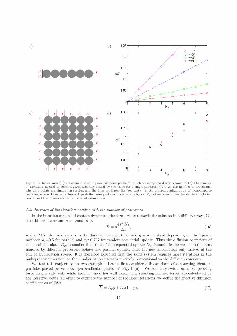
As a last check, we tested the physical properties of the system calculated by different number of pro-cessors. It is known that in the rigid limit, the force network of a given geometrical packing is not unique[29, 30]. Running the contact dynamics with different random seeds (for the random sequential update) leadsto different sets of contact forces, which all ensure the dynamical equilibrium. The domain decompositionalso changes the update order and the solutions will be microscopically different. Thus, a direct comparisonis impossible and we have to resort to comparing distributions.

We first investigate the distribution of the contact force orientations f(φ) in the relaxed system of 8000particles described in Sec. 4.1. The contact forces are calculated from scratch for the given geometry andboundary conditions using different number of processors. Since the system is very tall (Ly/Lx=16), it isdivided only vertically for up to Np=16, while for Np=32 the 16 domains are cut horizontally as well. Thedistributions of the contact force orientations, fN

p(φ), are compared for several values of Np in Fig. 14(a).

16

0 100 200 300y / ( 2 r

max)

-1.2

-1

-0.8

σ yy /

P ext

sequentialparallel , N

p=3

y=107 y=212domain boundaries at: and

Figure 15: (color online) σyy(y) scaled by the external pressure Pext in terms of the height y scaled by the diameter of thelargest particle in the system (2 rmax). The results obtained by the non-parallel code are compared with those obtained by theparallel code for Np = 3.

For comparison, we have presented the results of the simulations with Np=1 for two different random seedsas well. The match among the different runs are so good that the curves coincide. Hence, we also plot therelative difference fN

p(φ)/f1(φ)−1 to the non-parallel run for comparison, which shows negligible random

noise. Evidently, parallelization has no systematic impact on the angular distribution of the contact forces.Similar results were obtained when the system is sheared by the horizontal confining walls moving with aconstant velocity in opposite directions as shown in Fig. 14(b).

We also calculate the σyy component of the stress tensor as a function of the distance y from the bottomwall in the same system. σyy(y) at a given height y is averaged over a horizontal stripe of width dy=2rmax,where rmax is the largest particle radius in the system. The system height is thus divided into nearly 320stripes. Figure 15 displays the results obtained by the non-parallel code as well as the parallel code withNp=3. In the parallel case, the system is divided horizontally into three parts. The results of the parallelrun match perfectly with the one of the non-parallel run. Especially, no kind of discontinuity or anomaly isobserved at y ≃ 107 and y ≃ 212, where the interfaces between the processors are located.

5. Conclusion and Discussion

We have presented an efficient parallel version of contact dynamics method in this work, which allowsfor large-scale granular simulations with almost 100% efficiency. We aimed at the full parallelization of thecode with hierarchical domain decomposition and dynamical load balancing, in which the interface areabetween subdomains is also minimized. The parallel code is hence applicable to a broad range of densitiesand different simulation conditions.

The force calculation in CD is done by an iterative scheme, which shows an instability if more than abouthalf of the contacts are calculated in parallel. The iteration scheme was kept domain-wise sequential whiledata across the domain boundaries are exchanged after every iteration, ensuring that the iteration is stablefor all system sizes. It is known that the CD iterative scheme approaches the solution in a diffusive manner.The diffusion constant is smaller for parallel update, which happens at domain boundaries. However, thisoverhead is proportional to the square root of the number of processors divided by the number of particles(in 2D), which vanishes for large systems.

The other point of discussion raised here concerns the choice of the mesh size and adjusting the subdomainborders to it. Communication overhead was reduced because between iteration steps not all boundaryinformation is sent but only the relevant part of it. The subdomain wall position is only important if theparticle size is not small compared to the system size. For large scale parallel applications this can onlybe a problem for highly polydisperse systems, for which the cell method for contact detection breaks downanyway.

17

The load balancing is done only after a full iteration scheme at the end of each time step. Our inves-tigations show that this happens rarely enough that load balancing overhead and CPU time fluctuationsare negligible but often enough to achieve fast load balance. We used a global criterion for stopping theiteration scheme. This ensures that the physical properties of the tested samples do not show any differencecompared to the non-parallel version of the code.

Blocking point-to-point communications were used to transfer data among processors. Since our algo-rithm needs synchronization after each iteration, non-blocking data transfer would not be advantageous.The whole amount of data is transmitted in one single packet, which reduces communication overhead overthe pure data. This method introduces parallel contact update at domain boundaries, which induces aniteration number overhead due to the lower diffusivity of the information in parallel update. This overheadvanishes, e.g. with the square root of the processor number over particle number in two dimensions, whichis in general negligible.

An alternative method would be to use non-blocking communications for the iteration scheme, namelyto immediately send a freshly updated contact force in the vicinity of the borders to the correspondingprocessors, while on the other side this would trigger an interrupt when the other processor immediatelyupdates the received contact data. This prevents the mixture of sequential and parallel update schemes.However, we do not expect that the performance of the method is greatly enhanced by the use of non-blocking communication because the information of each contact force is sent individually and the overheadassociated with the increase of the inter-processor communications significantly affects the performance.

The last point to discuss concerns the load balancing method. The most exact method would be toconsider the number of particles and/or contacts in each subdomain to calculate their new boundaries.Practically, this would cause difficulties, since each processor is just aware of particles and contacts withinits own borders. The amount of calculations and communications between neighboring processors to placethe interface according to the current contact and particle positions would make the load balancing acomputationally expensive process. This lead us to balance the load further by dividing the simulationdomain according to the current subdomain volumes (not always proportional to the number of particlesand/or contacts), which is in fact a control loop with the inherent problems of under- and over-damping.

Acknowledgments

We would like to thank M. Magiera, M. Gruner and A. Hucht for technical support and useful discussions,and M. Vennemann for comments on the manuscript. Computation time provided by John-von-NeumannInstitute of Computing (NIC) in Julich is gratefully acknowledged. This research was supported by DFGGrant No. Wo577/8 within the priority program “Particles in Contact”.

References

[1] P. A. Cundall, O. D. L. Strack, A discrete numerical model for granular assemblies, Geotechnique 29 (1979) 47-65.[2] S. Luding, Molecular dynamics simulations of granular materials, in: The Physics of Granular Media, Wiley-VCH, Wein-

heim, 2004, pp. 299-324.[3] D. C. Rapaport, The event scheduling problem in molecular dynamic simulation, J. Comp. Phys. 34 (1980) 184-201.[4] O. R. Walton, R. L. Braun, Viscosity, granular-temperature, and stress calculations for shearing assemblies of inelastic,

frictional disks, Journal of Rheology 30 (1986) 949-980.[5] M. Jean, J. J. Moreau, Unilaterality and dry friction in the dynamics of rigid body collections, in: Proc. of Contact

Mechanics Intern. Symposium, Presses Polytechniques et Universitaires Romandes, Lausanne, Switzerland, 1992, pp.31-48.

[6] J. J. Moreau, Some numerical-methods in multibody dynamics - application to granular-materials, Eur. J. Mech. A-Solids13 (1994) 93-114.

[7] M. Jean, The non-smooth contact dynamics method, Comput. Methods Appl. Mech. Engrg. 177 (1999) 235-257.[8] L. Brendel, T. Unger, D. E. Wolf, Contact dynamics for beginners, in: The Physics of Granular Media, Wiley-VCH,

Weinheim, 2004, pp. 325-343.[9] S. Plimpton, Fast parallel algorithms for short-range molecular dynamics, J. Comp. Phys. 117 (1995) 1-19.

[10] L. Nyland, J. Prins, R. H. Yun, J. Hermans, H.-C. Kum, L. Wang, Achieving Scalable Parallel Molecular Dynamics UsingDomain Decomposition Techniques, J. Parallel Distrib. Comput. 47 (1997) 125-138.

18

[11] Y. Deng, R. F. Peierls, C. Rivera, An adaptive load balancing method for parallel molecular dynamics simulations, J.Comp. Phys. 161 (2000) 250-263.

[12] S. J. Plimpton, Fast Parallel Algorithms for Short-Range Molecular Dynamics, J Comp Phys, 117, (1995) 1-19.[13] P. K. Haff, Grain flow as a fluid-mechanical phenomenon, J. Fluid Mech. 134 (1983) 401-430.[14] S. McNamara, W. R. Young, Inelastic collapse in two dimensions, Phys. Rev. E 50 (1994) R28-R31.[15] S. Miller, S. Luding, Event-driven molecular dynamics in parallel, J. Comp. Phys. 193, (2003) 306-316.[16] P. Breitkopf, M. Jean, Modelisation parallele des materiaux granulaires, in: 4eme colloque national en calcul des structures,

Giens, 1999, pp. 387-392.[17] M. Renouf, F. Dubois, P. Alart, A parallel version of the non smooth cantact dynamics algorithm applied to the simulation

of granular media, J. Comput. Appl. Math. 168 (2004) 375-382.[18] V. Zhakhovskii, K. Nishihara, Y. Fukuda, S. Shimojo, A new dynamical domain decomposition method for parallel

molecular dynamics simulation on grid, in: Annual Progress Report, Institute of Laser Engineering, Osaka University,2004.

[19] J. K. Salmon, Parallel hierarchical N-body methods, Ph.D. Thesis, Caltech University, Pasadena, U.S.A., 1990.[20] M. S. Warren, J. K. Salmon, A parallel hashed oct-tree N-body algorithm, in: Proceedings of Supercomputing 93, 1993,

pp. 12-21.[21] F. Fleissner, P. Eberhard, Parallel load-balanced simulation for short-range interaction particle methods with hierarchical

particle grouping based on orthogonal recursive bisection, Int. J. Numer. Meth. Engng 74 (2008) 531-553.[22] T. Unger, L. Brendel, D. E. Wolf, J. Kertesz, Elastic behavior in contact dynamics of rigid particles, Phys. Rev. E 65

(2002) 061305.[23] M. R. Shaebani, T. Unger, J. Kertesz, Generation of homogeneous granular packings: Contact dynamics simulations at

constant pressure using fully periodic boundaries, Int. J. Mod. Phys. C 20 (2009) 847-867.[24] W. Press, S. A. Teukolsky, W. T. Vetterling, B. P. Flannery, Numerical Recipes: The Art of Scientific Computing, Chapter

19, Cambridge University Press, Cambridge, 2007.[25] M.P. Allen, D.J. Tildeslay, Computer Simulation of Liquids, Oxford University Press, Oxford, 1987.[26] M. Wackenhut, S. McNamara, H. Herrmann, Shearing behavior of polydisperse media, Eur. Phys. J. E 17 (2005) 237-246.[27] V. Ogarko, S. Luding, Data structures and algorithms for contact detection in numerical simulation of discrete particle

systems, in: Proc. of World Congress Particle Technology 6, Nurnberg Messe GmbH (Ed.), Nuremberg, 2010.[28] S. Revathi, V. Balakrishnan, Effective diffusion constant for inhomogeneous diffusion, J. Phys. A: Math. Gen. 26 (1993)

5661-5673.[29] M. R. Shaebani, T. Unger, J. Kertesz, Extent of force indeterminacy in packings of frictional rigid disks, Phys. Rev. E 79

(2009) 052302.[30] T. Unger, J. Kertesz, Dietrich E. Wolf, Force indeterminacy in the jammed state of hard disks, Phys. Rev. Lett. 94 (2005)

178001.

19