University of WyomingWyoming Scholars Repository

Mathematics Faculty Publications Mathematics

5-1-1998

Domain Decomposition Operator Splittings forthe Solution of Parabolic EquationsT. P. Mathew

Peter PolyakovUniversity of Wyoming, polyakov@uwyo.edu

G. Russo

J. Wang

Follow this and additional works at: http://repository.uwyo.edu/math_facpub

Part of the Mathematics Commons

This Article is brought to you for free and open access by the Mathematics at Wyoming Scholars Repository. It has been accepted for inclusion inMathematics Faculty Publications by an authorized administrator of Wyoming Scholars Repository. For more information, please contactscholcom@uwyo.edu.

Publication InformationMathew, T. P.; Polyakov, Peter; Russo, G.; and Wang, J. (1998). "Domain Decomposition Operator Splittings for the Solution ofParabolic Equations." SIAM Journal on Scientific Computing 19.3, 912-932.

DOMAIN DECOMPOSITION OPERATOR SPLITTINGSFOR THE SOLUTION OF PARABOLIC EQUATIONS∗

T. P. MATHEW† , P. L. POLYAKOV† , G. RUSSO‡ , AND J. WANG†

SIAM J. SCI. COMPUT. c© 1998 Society for Industrial and Applied MathematicsVol. 19, No. 3, pp. 912–932, May 1998 009

Abstract. We study domain decomposition counterparts of the classical alternating directionimplicit (ADI) and fractional step (FS) methods for solving the large linear systems arising from theimplicit time stepping of parabolic equations. In the classical ADI and FS methods for parabolicequations, the elliptic operator is split along coordinate axes; they yield tridiagonal linear systemswhenever a uniform grid is used and when mixed derivative terms are not present in the differentialequation. Unlike coordinate-axes-based splittings, we employ domain decomposition splittings basedon a partition of unity. Such splittings are applicable to problems on nonuniform meshes and evenwhen mixed derivative terms are present in the differential equation and they require the solution ofone problem on each subdomain per time step, without iteration. However, the truncation error inour proposed method deteriorates with smaller overlap amongst the subdomains unless a smaller timestep is chosen. Estimates are presented for the asymptotic truncation error, along with computationalresults comparing the standard Crank–Nicolson method with the proposed method.

Key words. domain decomposition, alternating direction implicit method, fractional stepmethod, operator splitting, parabolic equation, partition of unity

AMS subject classifications. 65N20, 65F10

PII. S1064827595288206

1. Introduction. The numerical solution of parabolic partial differential equa-tions by implicit time stepping procedures requires the solution of large systems of lin-ear equations. These linear systems need only be solved approximately, provided thatthe inexact solutions obtained by using approximate solvers preserve the stability andlocal truncation error of the original scheme. Though iterative methods with precon-ditioners are a popular way for solving such linear systems, see [5, 6, 3, 8, 15, 33, 4, 7],in this paper we consider only approximate solvers that do not involve iteration at eachtime step. Such approximate noniterative solution methods for parabolic equationsinclude the alternating direction implicit (ADI) methods of Peaceman and Rachford[22] and Douglas and Gunn [12], the fractional step methods (FS) of Bagrinovskii andGodunov [1], Yanenko [34], and Strang [26], and also more recent one-iteration domaindecomposition solvers of Kuznetsov [16, 17], Meurant [21], Dryja [13], Blum, Lisky,and Rannacher [2], Dawson, Du, and Dupont [9], Laevsky [19, 18] and Vabishchevich[28] and Vabishchevich and Matus [29], and Chen and Lazarov [20].

The method proposed here uses the same framework as the classical ADI and FSmethods for solving parabolic equations of the form ut + Lu = f using an operatorsplitting L = L1 + · · · + Lq; however, the splittings chosen here are based on domaindecomposition, unlike classical splittings along coordinate directions. Furthermore,they are applicable to problems with mixed derivative terms and on nonuniform grids.The basic idea is simple. Given a smooth partition of unity {χk}k=1,...,q subordinateto a decomposition of the domain, as described in section 4, an elliptic operator L,

∗Received by the editors June 26, 1997; accepted for publication (in revised form) July 12, 1996.http://www.siam.org/journals/sisc/19-3/28820.html

†Department of Mathematics, University of Wyoming, Laramie, WY 82071-3036(mathew@ledaig.uwyo.edu, polyakov@ledaig.uwyo.edu, junping@schwarz.uwyo.edu).

‡Dipartimento di Matematica, Universita dell’Aquila, Via Vetoio, Loc Coppito, 67010 L’Aquila,Italy (russo@smaq20.univaq.it).

912

DOMAIN DECOMPOSITION OPERATOR SPLITTINGS 913

such as the two-dimensional Laplacian, is split as a sum of several “simpler” operators:

Lu = −Δu = (L1 + · · · + Lq)u, where Liu = −∇ · χi∇u.

Given a splitting, an approximate solution of the parabolic equation is obtained bysolving several “simpler” evolution equations of the form ut + Lku = fk; see section3. By comparison, classical splittings, see Richtmyer and Morton [23], of L = −Δ areof the form L1 = − ∂2

∂x2 and L2 = − ∂2

∂y2 .Our goal in this paper is to derive truncation error estimates of the proposed

methods and to discuss their stability properties. The rest of the paper is outlinedas follows. In section 2, we describe a parabolic equation and its discretization. Insection 3, we describe the classical ADI and FS methods in matrix language. Insection 4, we describe domain decomposition operator splittings using a partition ofunity and derive asymptotic truncation error bounds and stability properties for theproposed method. A heuristic comparison is then made between the Crank–Nicolsonmethod and the ADI method with domain decomposition splitting. Finally, in section5, numerical results are presented.

2. A parabolic equation and its discretization. We consider the followingparabolic equation for u(x, y, t) on a domain Ω ⊂ R2:⎧⎨

⎩ut = ∇ · a(x, y)∇u − c(x, y)u + f(x, y, t), in Ω × [0, T ],

u(x, y, 0) = u0(x, y), in Ω,u(x, y, t) = 0, on ∂Ω × [0, T ],

where a(x, y) is a 2 × 2 symmetric positive definite matrix function with C2q−1(Ω)entries, c(x, y) ≥ 0 is in C2q(Ω), f(x, y, t) is a C2q(Ω×[0, T ]) forcing term, and u0(x, y)is a C2q(Ω) initial data. Here q is an integer to be specified later in section 4. Withthese smoothness assumptions, the exact solution u(x, y, t) will be in C2q(Ω × [0, T ]).We will denote the elliptic operator by Lu = −∇ · a(x, y)∇u + c(x, y)u, and theparabolic equation by ut + Lu = f .

2.1. Discrete problem. Let Ah denote the symmetric positive definite matrixobtained by second-order finite difference discretization of the elliptic operator L ona grid on Ω with mesh size h and grid points (xi, yj):

(AhU)ij = Lu(xi, yj) + O(h2),

where Uij ≈ u(xi, yj , t) denotes the discrete solution. To discretize in time, we applyan implicit scheme such as the backward Euler or Crank–Nicolson scheme, whichresults in a large sparse linear system to be solved.

For example, the backward Euler method yields

Un+1 − Un

τ= −AhUn+1 + Fn+1, or (I + τAh) Un+1 = Un + τFn+1,(1)

where τ is the time step, Un = {U(xi, yj , nτ)} denotes the vector of discrete unknownsat time tn = nτ , and Fn = {f(xi, yj , nτ)} is the discrete forcing term at time tn. Asis well known, see [23], the above scheme is unconditionally stable in the Euclideannorm ‖.‖ and convergent with error: ‖u − Ube‖ = O (τ) + O

(h2

). Thus, for transient

problems τ = O(h2) provides an optimal choice of time step τ for the backward Eulermethod.

914 T. MATHEW, P. POLYAKOV, G. RUSSO, AND J. WANG

Similarly, the Crank–Nicolson method yields

Un+1 − Un

τ= −Ah

(Un+1 + Un

2

)+

(Fn+1 + Fn

2

),(2)

which requires the solution of the linear system

(I +

τ

2Ah

)Un+1 =

(I − τ

2Ah

)Un + τ

(Fn+1 + Fn

2

).(3)

The Crank–Nicolson method is also unconditionally stable, see [23], with error: ‖u −Ucn‖ = O

(τ2

)+ O

(h2

)yielding second-order convergence when τ = O(h).

We note that both of the above discretizations can be written in the form

(I + ατAh) Un+1 + BUn = gn,(4)

for suitable choices of constants α, matrices B, and forcing terms gn. In particular,the coefficient matrices can be written in the form I + ατAh for α = 1 or α = 1

2 , andthey are symmetric positive definite. Furthermore, since it is known that the largesteigenvalue of Ah satisfies λmax(Ah) = O(h−2), it follows that the condition numberof I + ατAh is bounded by 1 + cτh−2, for some positive constant c independent ofτ and h. Thus, for h2 � τ � 1 systems (1) and (3) are ill conditioned, yet betterconditioned than Ah. Consequently, if iterative methods are used, preconditionerssuch as multigrid [4, 15] or domain decomposition methods may be needed to reducethe number of iterations; see, for example, [5, 6, 3, 8, 33, 7].

However, as mentioned earlier, system (4) for Un+1 needs only to be solved ap-proximately within the local truncation error. In this paper we only seek solvers thatprovide approximate solutions at the cost of one iteration per time step. Such ap-proximate solvers will modify the scheme (4) and alter its stability and truncationerror. In order to distinguish this with the modified schemes, we will henceforth re-fer to scheme (4) as the original scheme. In sections 3 and 4, we discuss one-stepapproximate solvers, and estimate their truncation errors using the framework of theclassical ADI and FS methods. We also describe conditions under which the stabilityof the original scheme is preserved.

Given the original discretization (4), we define its local truncation error Torig asfollows:

Torig = (I + ατAh) un+1 + Bun − gn,(5)

where u is the exact solution of the parabolic equation restricted to the grid points.Discretization (4) is said to be stable in a norm ‖ · ‖ if the following holds for somenumbers c1, c2:

‖Un+1‖ ≤ (1 + c1τ)‖Un‖ + c2‖gn‖.

If c1 and c2 are independent of h and τ , then the discretization is said to be uncon-ditionally stable, else conditionally stable.

3. ADI and FS methods. Given an evolution equation of the form ut+Lu = f ,the basic idea in the ADI and FS methods is to approximately solve it using anoperator splitting L = L1 + · · · + Lq, where several simpler evolution equations of theform wt + Liw = fi are solved with suitably chosen fi to provide an approximatesolution w ≈ u to the original equation.

DOMAIN DECOMPOSITION OPERATOR SPLITTINGS 915

We will henceforth restrict our discussion to the matrix case, where a discretiza-tion in space of ut + Lu = f yields Ut + AhU = Fh, and a subsequent discretizationin time yields system (4). Corresponding to an operator splitting L = L1 + · · · + Lq,where q > 1, we assume a matrix splitting of Ah as a sum of symmetric positivesemidefinite matrices Ai:

Ah = A1 + · · · + Aq, where Ai ≥ 0.(6)

It will be assumed that the matrices Ai have a “simpler” structure than Ah, in thesense to be explained below.

In matrix language, given the splitting {Ai}, both the ADI and FS methodsapproximately solve systems of the form (I + ατAh)w = z by solving several systemsof the form (I + ατAi)wi = zi; see sections 3.1 and 3.2. Hence, the Ai must besuitably chosen so that the latter systems are easier to solve than the original system.

As an example of splittings, we briefly describe the classical splittings, see [23], ofan elliptic operator along the x and y coordinate directions (when no mixed derivativeterms are present). Domain decomposition splittings are described in section 4. Forclassical splittings, the two-dimensional Laplacian L = −Δ is split as a sum of L1 =− ∂2

∂x2 and L2 = − ∂2

∂y2 . In matrix terms

Ah = −Δh = −Dhxx − Dh

yy,

where Δh denotes the discrete Laplacian and Dhxx and Dh

yy denote the discretizationof ∂2

∂x2 and ∂2

∂y2 , respectively. Both A1 = −Dhxx and A2 = −Dh

yy will be tridiagonalmatrices after a suitable ordering of the unknowns (if the grid is uniform) and hence(I + ατAi) will also be tridiagonal and solvable in linear time on uniform grids!

Unfortunately, such splittings are not possible if mixed derivative terms arepresent and tridiagonality can be lost if the grid is nonuniform. By contrast, thedomain decomposition splittings described in section 4 are applicable in more generalcases, though the resulting linear systems are not tridiagonal.

3.1. ADI method. This method was originally proposed by Peaceman andRachford [22] and Douglas [11, 10], and was further developed by several authors. Wefollow here the general formulation described by Douglas and Gunn [12], where addi-tional references may be found. The reader is also referred to [30, 31, 32, 14, 24, 27].In matrix language, given a splitting Ah = A1 + · · ·+Aq and an approximate solutionWn ≈ Un to the discrete solution at time tn, an approximate solution Wn+1 ≈ Un+1

of the linear system

(I + ατAh) Un+1 = gn − BUn

is obtained by solving systems of the form (I + ατAi) wi = zi as follows.ADI ALGORITHM.1. Given Wn, solve for Wn+1

1 :

(I + ατA1) Wn+11 +

q∑j=2

ατAjWn + BWn = gn.

2. For i = 2, . . . , q, solve for Wn+1i :

(I + ατAi) Wn+1i − Wn+1

i−1 − ατAiWn = 0.

916 T. MATHEW, P. POLYAKOV, G. RUSSO, AND J. WANG

3. Define the ADI approximate solution at time tn+1 = (n + 1)τ to be

Wn+1 = Wn+1q .

We note that in order to compute Wn+1 in the ADI scheme, we need to solve a totalof q linear systems, each of the form I + ατAi of size n × n (the size of Ah). Thefollowing stability results for the ADI method can be found in [12].

THEOREM 3.1. If the matrices Ai are symmetric positive semidefinite for i =1, . . . , q, if B is symmetric, and if Ai and B commute pairwise, then the ADI schemeis unconditionally stable. In the noncommuting case, if q = 2 and if the matricesAi are symmetric positive semidefinite, and if ‖ · ‖ is any norm in which the originalscheme (4) is stable, then the ADI scheme is stable in the norm ‖|u‖| ≡ ‖(I+ατA2)u‖.For q ≥ 3, if the matrices Ai are positive semidefinite, then the ADI scheme can beshown to be conditionally stable.

For q ≥ 3 in the noncommuting case, examples are known of positive semidefinitesplittings for which the ADI method can loose unconditional stability; see [12]. Nev-ertheless, the above stability results are a bit pessimistic and instability is only rarelyencountered in practice.

Next, we describe the truncation error terms for the ADI method, derived in [12].The magnitude of these truncation terms will be estimated in section 4.3 for domaindecomposition splittings.

THEOREM 3.2. Given the discrete problem

(I + ατAh) Un+1 + BUn = gn,

with local truncation error Torig (see (5)), the ADI solution Wn+1 solves the followingperturbed problem:

(I + ατAh) Wn+1 +q∑

m=2

⎛⎝αmτm

∑1≤σ1<···<σm≤q

Aσ1 · · ·Aσm

(Wn+1 − Wn

)⎞⎠+BWn = gn,

(7)

which introduces the following additional terms in the local truncation error:

Tadi = Torig +q∑

m=2

⎛⎝αmτm

∑1≤σ1<···<σm≤q

Aσ1 · · ·Aσm

(un+1 − un

)⎞⎠ ,(8)

where u is the exact solution of the parabolic equation restricted to the grid points.Proof. The proof is given in [12]; however, for completeness we include it here.

From step 2 of the ADI algorithm, we obtain that Wn+1i satisfies

(I + ατAi) (Wn+1i − Wn) = Wn+1

i−1 − Wn for i = 2, . . . , q.

By recursively applying this, we deduce that

(I + ατA2) · · · (I + ατAq) (Wn+1q − Wn) = (Wn+1

1 − Wn).(9)

Now, from step 1 of the ADI algorithm, we deduce that

(I + ατA1) (Wn+11 − Wn) = gn − BWn − ∑q

j=2 ατAjWn − (I + ατA1) Wn

= gn − BWn − (I + ατAh)Wn.(10)

DOMAIN DECOMPOSITION OPERATOR SPLITTINGS 917

Multiplying (9) by (I + ατA1) and substituting (10) for the resulting right-hand side,we obtain

(I + ατA1) · · · (I + ατAq) (Wn+1q − Wn) = gn − BWn − (I + ατAh)Wn.(11)

Noting that

(I + ατA1) · · · (I + ατAq) = I + ατAh +q∑

m=2

αmτm

⎛⎝ ∑

1≤σ1<···<σm≤q

Aσ1 · · ·Aσm

⎞⎠ ,

(7) follows.Explicit estimates of these truncation error terms for the case of domain decom-

position splittings are given in section 4.3.

3.2. FS methods. These methods were originally developed by Bagrinovskiiand Godunov [1] and Yanenko [34] and further developed by Strang [26] and otherauthors. Given a matrix splitting Ah = A1 + · · · + Aq, the FS methods approximate(I + ατAh) by a product of several matrices of the form (I + ατAi). For example,the first-order FS method uses the approximation

(I + ατAh) = (I + ατA1) · · · (I + ατAq) + O(τ2),(12)

which can be formally verified by multiplying all the terms, bearing in mind that thematrices Ai may not commute. Given (12), an approximate solution Wn+1 ≈ Un+1

of

(I + ατAh) Un+1 + BUn = gn(13)

can be obtained by solving

(I + ατA1) · · · (I + ατAq) Wn+1 = gn − BWn.(14)

We summarize below the first-order fractional step algorithm to approximately solve(I + ατAh)Un+1 = gn − BUn with Wn+1

fs ≈ Un+1.FIRST-ORDER FS ALGORITHM.1. Let z1 = gn − BWn and for i = 1, . . . , q solve

(I + ατAi)wi = zi, and define zi+1 = wi.

2. Let Wn+1fs = wq.

Though (14) is a second-order approximation (locally) in τ of (13), it is only first-order accurate globally, due to accumulation of errors; see [23]. The following resultconcerns the stability of the first-order FS method.

THEOREM 3.3. If Ai are symmetric and positive semidefinite, and if ‖B‖ ≤ 1 inthe Euclidean norm ‖.‖, then the first-order FS method is stable with

‖Wn+1‖ ≤ ‖Wn‖ + c‖gn‖for some c > 0 and independent of τ and h.

Proof. Since Wn+1 = (I+ατAq)−1 · · · (I+ατA1)−1 (gn − BWn) and since ‖B‖ ≤1 in the spectral norm, we only need verify that

‖ (I + ατAq)−1 · · · (I + ατA1)

−1 ‖ ≤ 1

918 T. MATHEW, P. POLYAKOV, G. RUSSO, AND J. WANG

in the spectral norm. But this follows easily: since each of the terms (I + ατAi) aresymmetric positive definite with eigenvalues greater than one, the spectral norms oftheir inverses are each bounded by one.

The following result concerns the local truncation error of the first-order FSmethod.

THEOREM 3.4. The first-order FS approximate solution Wn+1 of

(I + ατAh)Un+1 = gn − BUn

solves

(I + ατAh)Wn+1 +∑q

m=2

(αmτm

∑1≤σ1<···<σm≤q Aσ1 · · ·Aσm

)Wn+1

= gn − BWn.(15)

The local truncation error Tfs of the first-order FS method has the following terms inaddition to the terms in the local truncation error Torig when exact solvers are used:

Tfs = Torig +q∑

m=2

⎛⎝αmτm

∑1≤σ1<···<σm≤q

Aσ1 · · ·Aσm

⎞⎠ un+1.(16)

Here un+1 is the exact solution of the parabolic equation at time (n + 1)τ restrictedto the grid points.

Proof. Since the product

(I + ατA1) · · · (I + ατAq) = I + ατAh +q∑

m=2

⎛⎝αmτm

∑1≤σ1<···<σm≤q

Aσ1 · · ·Aσm

⎞⎠ ,

the proof immediately follows by replacing (I + ατAh) by (I + ατA1) · · · (I + ατAq)in the original discretization.

For a given splitting {Ai}, the above local truncation error terms are O(τ2)(though the constant in the leading-order term τ2 can vary for different choices ofsplittings). However, the global error will be O(τ), see [23], due to accumulation oferrors, and consequently, the above first-order FS method is suitable only for glob-ally first-order schemes such as backward Euler but not for globally second-orderdiscretizations such as Crank–Nicolson.

For globally second-order accurate schemes such as Crank–Nicolson, second-orderfractional step approximations can be obtained by using Strang splitting [26]. Weoutline the main idea for a splitting involving two matrices: Ah = A1 + A2. The aimis to approximate e−ατAh by a locally third-order accurate approximation as follows:

e−τAh = e− τ2 A1e−τA2e− τ

2 A1 + O(τ3).(17)

Then, as in the Crank–Nicolson method, a locally third-order approximation in τ ofthe terms e−ατAi can be used to replace each of the exponentials

e−ατAi =(I +

ατ

2Ai

)−1 (I − ατ

2Ai

)+ O(τ3).

Applying this to each of the terms in (17) yields the implementation of Strang splitting.We state without proof the following.

DOMAIN DECOMPOSITION OPERATOR SPLITTINGS 919

THEOREM 3.5. Strang splitting provides unconditionally stable approximationswhen Ai are symmetric positive semidefinite: Ai ≥ 0. For any fixed choice of positivesemidefinite matrices A1 and A2, the truncation error for Strang splitting is third-order accurate locally in τ , and globally second-order accurate in τ .

Since Strang splitting provides a globally second-order accurate approximation intime, it can be applied to inexactly solve the Crank–Nicolson scheme. However, it ismore expensive and complicated to generalize when there are more than two matricesin the splitting, and it requires more linear systems to be solved than the first-orderFS method. In the applications we consider, the ADI methods which were describedearlier are preferable and generate smaller truncation errors, though they are notguaranteed to be unconditionally stable without additional assumptions.

4. Domain-decomposition-based operator splittings. In this section, wedescribe domain-decomposition-based splittings

Ah = A1 + · · · + Aq

of the discretization Ah of L such that (I + ατAi)wi = zi can be solved at the costof solving a problem on a subdomain. For such splittings, we provide in section 4.3an explicit estimate on how the truncation error depends on the overlap β amongstthe subdomains. For related algorithms, we refer the reader to Dryja [13], Laevsky[19, 18], Vabishchevich [28] and Vabishchevich and Matus [29], Kuznetsov [17, 16],Blum, Lisky, and Rannacher [2], Meurant [21], Dawson, Du, and Dupont [9], andChen and Lazarov [20].

As noted in the introduction, given a smooth partition of unity {χk(x, y)}k=1,...,q

subordinate to a collection of open subdomains {Ω∗k}k=1,...,q which cover Ω, we split

an elliptic operator L as a sum of several “simpler” operators as follows:

Lu = −∇ · a(x, y)∇u + c(x, y)u=

∑qk=1 −∇ · (χk(x, y)a(x, y)∇u) + χk(x, y)c(x, y)u

= L1u + · · · + Lqu,(18)

where Lku = −∇· (χk(x, y)a(x, y)∇u)+χk(x, y)c(x, y)u. In what follows, we will de-note the coefficients of Lk by ak(x, y) = χk(x, y)a(x, y) and ck(x, y) = χk(x, y)c(x, y).For numerical purposes, we could replace a smooth partition of unity by one whichis piecewise smooth. In such a case, it may be necessary to define the operators Lk

weakly using a variational approach. The matrices Ak are obtained by discretizationof Lk.

4.1. Partition of unity. Given an overlapping collection of open subregions{Ω∗

k}k=1,...,q whose union contains Ω, a partition of unity subordinate to this coveringis a family of q nonnegative, C∞(Ω) smooth functions {χk(x, y)}k=1,...,q whose sumequals one and such that χk(x, y) vanishes outside Ω∗

k:

0 ≤ χk(x, y) ≤ 1, χ1(x, y) + · · · + χq(x, y) = 1, supp (χk(x, y)) ⊂ Ω∗k.

For numerical purposes, we will consider χk(x, y) which are not necessarily C∞(Ω)but are continuous and piecewise smooth. We will refer to such a partition of unityas piecewise smooth. For more information on partitions of unity, see Sternberg [25].

Construction of piecewise smooth partitions of unity. Given a collection ofoverlapping subdomains {Ω∗

k}k=1,...,q which form a covering of Ω, we wish to describehow a piecewise smooth partition of unity can be constructed. However, first wedescribe how to construct an overlapping covering {Ω∗

k}k=1,...,q.

920 T. MATHEW, P. POLYAKOV, G. RUSSO, AND J. WANG

Ω1

Ω5

Ω9

Ω13

Ω2

Ω6

Ω10

Ω14

Ω3

Ω7

Ω11

Ω15

Ω4

Ω8

Ω12

Ω16

16 Subdomains

Ω∗1

Ω∗9

Ω∗3

Ω∗11

Color 1

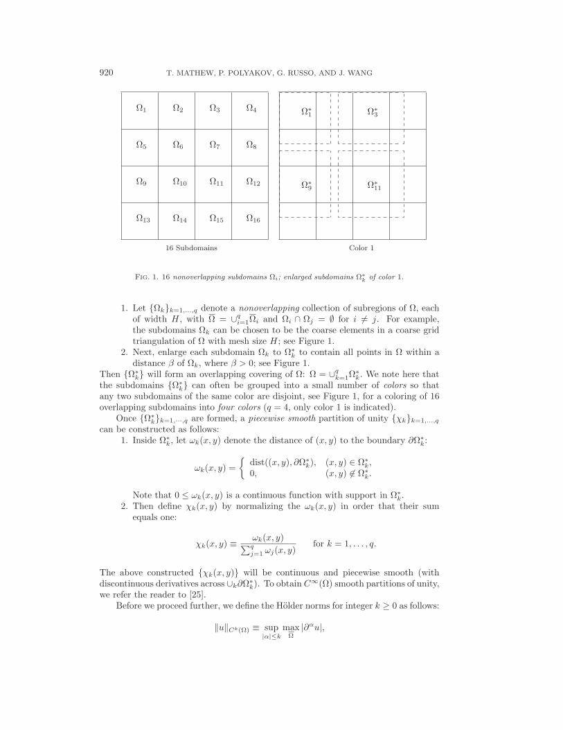
FIG. 1. 16 nonoverlapping subdomains Ωi; enlarged subdomains Ω∗k of color 1.

1. Let {Ωk}k=1,...,q denote a nonoverlapping collection of subregions of Ω, eachof width H, with Ω = ∪q

i=1Ωi and Ωi ∩ Ωj = ∅ for i = j. For example,the subdomains Ωk can be chosen to be the coarse elements in a coarse gridtriangulation of Ω with mesh size H; see Figure 1.

2. Next, enlarge each subdomain Ωk to Ω∗k to contain all points in Ω within a

distance β of Ωk, where β > 0; see Figure 1.Then {Ω∗

k} will form an overlapping covering of Ω: Ω = ∪qk=1Ω

∗k. We note here that

the subdomains {Ω∗k} can often be grouped into a small number of colors so that

any two subdomains of the same color are disjoint, see Figure 1, for a coloring of 16overlapping subdomains into four colors (q = 4, only color 1 is indicated).

Once {Ω∗k}k=1,···,q are formed, a piecewise smooth partition of unity {χk}k=1,...,q

can be constructed as follows:1. Inside Ω∗

k, let ωk(x, y) denote the distance of (x, y) to the boundary ∂Ω∗k:

ωk(x, y) ={

dist((x, y), ∂Ω∗k), (x, y) ∈ Ω∗

k,0, (x, y) ∈ Ω∗

k.

Note that 0 ≤ ωk(x, y) is a continuous function with support in Ω∗k.

2. Then define χk(x, y) by normalizing the ωk(x, y) in order that their sumequals one:

χk(x, y) ≡ ωk(x, y)∑qj=1 ωj(x, y)

for k = 1, . . . , q.

The above constructed {χk(x, y)} will be continuous and piecewise smooth (withdiscontinuous derivatives across ∪k∂Ω∗

k). To obtain C∞(Ω) smooth partitions of unity,we refer the reader to [25].

Before we proceed further, we define the Holder norms for integer k ≥ 0 as follows:

‖u‖Ck(Ω) ≡ sup|α|≤k

maxΩ

|∂αu|,

DOMAIN DECOMPOSITION OPERATOR SPLITTINGS 921

where we have used the multi-index notation

∂α =∂|α|

∂xα1∂yα2, α = (α1, α2).

For smooth partitions of unity with overlap β, the following result holds.PROPOSITION 4.1. Given a suitable collection of overlapping subregions,

{Ω∗k}k=1,...,q with overlap β, there exists a smooth partition of unity {χk(x, y)}k=1,...,q

satisfying

‖χk‖Cm(Ω) ≤ cmβ−m(19)

in the Holder Cm(Ω) norm, where cm > 0 is a constant independent of k and β butdependent on the geometry of the region.

Proof. We sketch the main ideas.1. First, map Ω to an enlarged region Ω using the change of variables (x, y) =

(x/β, y/β). This mapping enlarges Ω, and consequently all its subregions{Ω∗

k}, by a factor of β−1. Denote by {Ω∗k}k=1,...,q the corresponding covering

of Ω. These subregions will have an overlap parameter of size O(1).2. Next, construct a C∞(Ω) partition of unity {χk}k=1,...,q on Ω, subordinate

to the covering {Ω∗k}k=1,...,q; see for instance Sternberg [25]. This partition of

unity on Ω defines a corresponding C∞(Ω) partition of unity on Ω as follows:

χk(x, y) ≡ χk(x, y) for k = 1, . . . , q.

3. By repeated applications of the chain rule, it follows that

∂|α|χk

∂xα1∂yα2= β−|α| ∂|α|χk

∂xα1∂yα2.

Using the definition of the Holder norm it follows that

‖χk‖Cm(Ω) ≤ β−m‖χk‖Cm(Ω) = cmβ−m,

where cm is defined by cm ≡ ‖χk‖Cm(Ω).We omit further details.

For numerical implementation, smooth partitions of unity can be replaced bypiecewise smooth ones based on the distance functions wk(x, y). See section 5 for anexample of an alternative partition of unity for rectangular subdomains.

4.2. Domain decomposed matrix splittings. As mentioned before, given apartition of unity {χk}k=1,...,q as in section 4.1, a domain decomposition splitting ofthe operator Lu = −∇·a(x, y)∇u−c(x, y)u is obtained as Lku = −∇· (ak(x, y)∇u)+ck(x, y)u(x, y). By construction,

∑qk=1 Lk = L, and each Lk are self-adjoint. Ak

are then defined as suitable discretizations of the differential operators Lk, and soAh =

∑qk=1 Ak. We note that if c(x) ≥ 0, then each Lk and Ak will be positive

semidefinite. The Ak constructed above can then be used in the ADI and FS methodsdescribed in section 3, where the solution of (I +ατAk)w = z corresponds to solving aproblem on subregion Ω∗

k. Additionally, by coloring, problems on disjoint subregionsof the same color can be solved in parallel.

922 T. MATHEW, P. POLYAKOV, G. RUSSO, AND J. WANG

4.3. Truncation errors of the ADI and FS methods for domain decom-position splittings. As described in sections 3.1 and 3.2, when the ADI and FSmethods are used to approximately solve a discretization

(I + ατAh) Un+1 = gn − BUn,(20)

the resulting approximate solutions Wn+1adi and Wn+1

fs solve the perturbed problems (7)and (15), respectively. These perturbed problems correspond to new discretizationsof the original parabolic equation ut + Lu = f with additional truncation terms ofthe form τmAσ1 · · ·Aσm

(Wn+1 − Wn) and τmAσ1 · · ·AσmWn+1 for the ADI and FS

methods, respectively. Our goal in this section is to estimate the magnitude of theseadditional terms for the case of domain decomposition splittings.

As is well known, see for instance Richtmyer and Morton [23], once the localtruncation errors Tadi and Tfs are estimated, the global errors Eadi(t) = ‖u(t) −Wadi(t)‖ and Efs(t) = ‖u(t) − Wfs(t)‖ will follow by Lax’s convergence theorem, ifthe schemes are stable. We note, however, that the global error will be larger thanthe local truncation errors by a factor of τ−1 due to the accumulation of truncationerrors.

Since the local truncation errors Torig for the case of backward Euler or Crank–Nicolson with exact solvers are known, our estimates will focus on the new truncationterms Aσ1 · · ·Aσm

W and Aσ1 · · ·Aσm(Wn+1 − Wn). For simplicity, we will assume

that c(x, y) = 0 and that a(x, y) is a smooth scalar function. The analysis for thecases when c(x, y) ≥ 0 and for smooth matrix functions a(x, y) is similar. Our analysiswill require the following smoothness assumptions for the functions a(x, y), W (x, y, t),and {χk(x, y)}; a(x, y) should be in C2q−1(Ω), W (x, y, .) should be in C2q

0 (Ω), and{χk(x, y)} should be in C2q−1(Ω). With some abuse of notation, W will also refer toW = {W (xi, yj , .)}, the vector of nodal values of W (x, y, .) on the grid points of Ω.

Our estimates will be based on two simple observations, the details of which willbe provided subsequently.

1. The finite difference approximations Aσ1 · · ·AσmW (which occurs in Tfs) andAσ1 · · ·Aσm(Wn+1−Wn) (which occurs in Tadi) can be shown to be “similar”to their continuous counterparts Lσ1 · · ·LσmW and Lσ1 · · ·Lσm(Wn+1−Wn),respectively. This result is obtained by repeated applications of the integralform of the mean value theorem to the difference quotients.

2. Using step 1, the expressions Aσ1 · · ·AσmW and Aσ1 · · ·Aσm

(Wn+1 − Wn)can be estimated in terms of the maximum values of the derivatives of W andthe derivatives of the coefficients {ak(x, y)}. The derivatives of {ak(x, y)} canbe estimated in terms of the derivatives of a(x, y) and of the partition of unityfunctions {χk(x, y)}. Using the bounds (19) for the partition of unity, we canthen obtain that∣∣∣(Aσ1 · · ·AσmW )ij

∣∣∣ ≤ C(a)β−2m+1‖W‖C2m(Ω),

where C(a) is a positive constant that depends on the coefficients a(x, y) andits derivatives. Similar estimates will be valid for Aσ1 · · ·Aσm

(Wn+1 − Wn

)but with an additional factor of τ due to the difference in time Wn+1 − Wn.

Before we proceed, we introduce some notation. In addition to multi-index deriva-tives, ∂α = ∂|α|

∂xα1∂yα2 , we will use multi-index integrals

IxhF (xi, yj) =

1h

∫ xi+h

xi

F (ξ, yj)dξ.

DOMAIN DECOMPOSITION OPERATOR SPLITTINGS 923

Iterated integrals are defined as follows:

Ixxh F (xi, yj) =

1h2

∫ xi

xi−h

∫ ξ+h

ξ

F (η, yj)dηdξ.

We also define Ixh, 1

2as

Ixh, 1

2F (xi, yj) =

1h

∫ xi+ h2

xi− h2

F (ξ, yj)dξ.

Similar integrals are defined in y.We now outline the details of step 1. By repeatedly applying the integral form of

the mean value theorem (or the fundamental theorem of calculus), one can express allthe difference quotients in Aσ1 · · ·Aσm

W in terms of integrals of derivatives of W andintegrals of the derivatives of the coefficients aσk

(x, y). We have the following result.LEMMA 4.2. Let W ∈ C2m

0 (Ω) and let the expansion of Lσ1 · · ·LσmW be of theform

Lσ1 · · ·LσmW =

∑(α1,...,αm+1)

|α1|≤1|α1|+···+|αm+1|=2m

Cα1,...,αm+1 (∂α1aσ1) · · · (∂αmaσm) (∂αm+1W ) ,

where each Cα1,...,αm+1 = 0 or 1. Then, for W (x, y) the product Aσ1 · · ·AσmW satis-

fies

(Aσ1 · · ·AσmW )ij

=∑

(α1,...,αm+1)

|α1|≤1|α1|+···+|αm+1|=2m

Cα1,...,αm+1I∗h · · · I∗

h (I∗h∂α1aσ1) · · · (I∗

h∂αmaσm) (I∗

h∂αm+1W ) ,

where each of the I∗h terms (with at most 2m such terms) results from a suitable choice

of single or multiple integrals Ih.Proof. The proof will follow by induction on m. For m = 1, the standard five-

point finite difference approximation (AkW )i,j of LkW (xi, yj)

(AkW )i,j = −ak(xi+ h2 ,yj)

(Wi+1,j−Wi,j

h

)−ak(xi− h

2 ,yj)(

Wi,j−Wi−1,jh

)h

−ak(xi,yj+ h2 )

(Wi,j+1−Wi,j

h

)−ak(xi,yj− h

2 )(

Wi,j−Wi,j−1h

)h ,

satisfies

(AkW )i,j = −(

1h

∫ xi+ h2

xi− h2

∂ak

∂x (ξ, yj)dξ)(

1h

∫ xi+h

xi

∂W∂x (ξ, yj)dξ

)−ak(xi − h

2 , yj)(

1h2

∫ xi

xi−h

∫ ξ+h

ξ∂2W∂x2 (η, yj)dηdξ

)−

(1h

∫ yj+ h2

yj− h2

∂ak

∂y (xi, ξ)dξ)(

1h

∫ yj+h

yj

∂W∂y (xi, ξ)dξ

)−ak(xi, yj − h

2 )(

1h2

∫ yj

yj−h

∫ ξ+h

ξ∂2W∂y2 (xi, η)dηdξ

).

(21)

This follows trivially by repeatedly applying the fundamental theorem of calculus tothe difference quotients in the finite difference discretization. For instance, 1

h (Wi+1,j

924 T. MATHEW, P. POLYAKOV, G. RUSSO, AND J. WANG

−Wi,j) = 1h

∫ xi+1

xi

∂W∂x (ξ, yj)dξ, and similarly 1

h (Wi,j+1 −Wi,j) = 1h

∫ yj+1

yj

∂W∂y (xi, ξ)dξ.

Next, we subtract and add the terms ak(xi− h2 , yj) 1

h2

∫ xi+1

xi

∂W∂x (ξ, yj)dξ and ak(xi, yj+

h2 ) 1

h2

∫ yj+1

yj

∂W∂y (xi, ξ)dξ to the resulting terms in the discretization and apply the

fundamental theorem of calculus again. Result (21) follows.We can restate equation (21) using the multi-index derivative and integral nota-

tion as

(AkW )i,j = −(Ix

h, 12∂xak

)(Ix

h∂xW ) − ak(xi − h2 , yj)

(Ixxh ∂2

xW)

−(Iy

h, 12∂yak

)(Iy

h∂yW ) − ak(xi, yj − h2 )

(Iyyh ∂2

yW).

(22)

But this is just an expression for LkW with multi-index integrals applied to its terms.Consequently, our proof for the case m = 1 is complete.

For m ≥ 2, we use the induction hypothesis and assume that the result holdstrue for m − 1. We will then show that the result holds for m. To do this, defineV = Aσ2 · · ·Aσm

W . Then, by the induction hypothesis

V =∑

(α2,...,αm+1)

|α2|≤1|α1|+···+|αm+1|=2m−2

Cα2,...,αm+1Ih · · · Ih (Ih∂α2aσ2) · · · (Ih∂αmaσm) (Ih∂αm+1W ) .

Now, Aσ1V can be calculated by using (22) which involves first- and second-orderpartial derivatives of V (x, y) locally.

The resulting expression can be simplified by the following observation. Thepartial derivative operators ∂α “commute” with all the integral operators Ix

h , Iyh , etc.

The commutativity of ∂x and Iyh follows from the differentiation rule for integrals

depending on a parameter. The commutativity of ∂x and Ixh can be seen by the

following example:

∂xIxhF (x, yj) = ∂x

(1h

∫ x+h

x

F (ξ, yj)dξ

)=

1h

∫ x+h

x

∂ξF (ξ, yj)dξ = Ixh∂xF (x, yj).

When higher-order partial derivatives and iterated integrals are involved, they can behandled by repeated applications of the above. Consequently, all the partial deriva-tives can be moved inside the integrals.

When all the partial derivatives are moved inside the integrals, we obtain anexpression similar to Lσ1 · · ·Lσm

W but containing integrals of the terms. This givesthe desired result for m.

This completes the sketch of the proof of step 1. We obtain step 2 immediatelyfrom Lemma 4.2 by applying the mean value property of integrals.

LEMMA 4.3. The discretization (Aσ1 · · ·AσmW )ij satisfies

|(Aσ1 · · ·AσmW )ij | ≤∑

(α1,...,αm+1)

|α1|≤1|α1|+···+|αm+1|=2m

Cα1,...,αm+1‖aσ1‖Cα1 · · · ‖aσm‖Cαm ‖W‖Cαm+1 ,

where Cα1,...,αm+1 = 0 or 1.Proof. The mean value property of integrals yields∣∣∣∣∣ 1h

∫ xi+h

xi

F (ξ, yj)dξ

∣∣∣∣∣ ≤ maxξ∈[xi,xi+h]

|F (ξ, yj)|.

DOMAIN DECOMPOSITION OPERATOR SPLITTINGS 925

Applying this to all the integrals Ih in Lemma 4.2, we obtain that

|(Aσ1 · · ·AσmW )ij |

≤∑

(α1,...,αm+1)

|α1|≤1|α1|+···+|αm+1|=2m

Cα1,...,αm+1‖∂α1aσ1‖C0(Ω) · · · ‖∂αmaσm‖C0(Ω)‖∂αm+1Wσm‖C0(Ω)

≤∑

(α1,...,αm+1)

|α1|≤1|α1|+···+|αm+1|=2m

Cα1,...,αm+1‖aσ1‖C|α1|(Ω) · · · ‖aσm‖C|αm|(Ω)‖Wσm‖C|αm+1|(Ω).

This gives us the desired result.Using Leibnitz’s rule for partial differentiation of ak(x, y) = χk(x, y)ak(x, y) and

applying bounds (19) for the partition of unity, we deduce that

‖ak(x, y)‖Cp(Ω) ≤ C(a)‖a‖Cp(Ω)‖χk‖Cp(Ω)

≤ C(a)β−p.

Here C(a) is a constant that depends only on the coefficients a(x, y) and some of itsderivatives.

By substituting these results in Lemma 4.3, we obtain the following.COROLLARY 4.4. If W ∈ C2m

0 (Ω), the discretization (Aσ1 · · ·AσmW )ij satisfies

|(Aσ1 · · ·AσmW )ij | ≤ C(a)β−2m+1‖W‖C2m(Ω).

Similarly, the discretization(Aσ1 · · ·Aσm

(Wn+1 − Wn))ij

satisfies

| (Aσ1 · · ·Aσm(Wn+1 − Wn)

)ij

| ≤ C(a)τβ−2m+1 sup[0,tf ]

‖∂tW‖C2m(Ω).

This completes the details of step 2.We are finally able to estimate the local truncation errors and the global errors

of the ADI method with domain decomposition splitting.THEOREM 4.5. Let the exact solution u(x, y, t) of the parabolic equation be in

C2q0 (Ω) for each t ∈ [0, tf ] and in C1([0, tf ]) for each (x, y). Then the local truncation

error Tadi of the ADI method with domain decomposition splitting satisfies

‖Tadi‖L2(Ω) ≤ ‖Torig‖L2(Ω) + C(a)τ3(

1β3 +

τ

β5 + · · · +τ q−2

β2q−1

)sup[0,tf ]

‖∂tu‖C2q(Ω),

where Torig is the local truncation error of the original scheme (4) when exact solversare used. Whenever the ADI scheme is stable, the error Eadi(t) = u(t) − Wadi(t)satisfies

(23)

‖Eadi(t)‖L2(Ω) ≤ ‖Eorig(t)‖L2(Ω)+C(a)τ2(

1β3 +

τ

β5 + · · · +τ q−2

β2q−1

)sup[0,tf ]

‖∂tu‖C2q(Ω)

for t ∈ [0, tf ].

926 T. MATHEW, P. POLYAKOV, G. RUSSO, AND J. WANG

Proof. By (8), the local truncation error satisfies

Tadi = Torig +q∑

m=2

⎛⎝αmτm

∑1≤σ1<···<σm≤q

Aσ1 · · ·Aσm

(un+1 − un

)⎞⎠ .

Considering the Euclidean norm ‖ · ‖ of the above expression, and estimating theadditional terms using Corollary 4.4, we obtain

‖Tadi‖ ≤ ‖Torig‖ +√

nC(a)∑q

m=2 τm+1β−2m+1 sup[0,tf ] ‖∂tu‖C2m(Ω)

≤ ‖Torig‖ +√

nC(a)τ3(

1β3 + τ

β5 + · · · + τq−2

β2q−1

)sup[0,tf ] ‖∂tu‖C2q(Ω),

where n is the number of grid points in Ω. Multiplying the entire expression by hand using that h‖ · ‖ is equivalent to ‖ · ‖L2(Ω), we can replace h‖Tadi‖ and h‖Torig‖by ‖Tadi‖L2(Ω) and ‖Torig‖L2(Ω), respectively. The desired estimate for the localtruncation error then follows by noting that

√nh is proportional to the square root

of the area of Ω, which can be absorbed in C(a).The error follows from the local truncation error by an application of the Lax

convergence theorem.Remark 1. Each of the terms (∂α1aσ1) · · · (∂αmaσm

) (∂αm+1W ) will be zero inmost of Ω, more specifically, outside ∩m

k=1Ω∗σk

, and our proof has not taken this intoaccount. This is due to the compact support of the coefficients aσk

(x, y) in Ω∗σk

.However, we expect that an estimate taking this into account will be much morecomplicated. Consequently, our theoretical estimate for the truncation errors arepessimistic when compared with actual numerical results from section 5.

Remark 2. For a fixed choice of subdomains {Ω∗k} and partition of unity {χk},

the overlap β is fixed. Consequently, the above truncation error bounds for the ADImethod with domain decomposition splitting is asymptotically second order in time,i.e., as τ → 0

‖u(t) − Wadi(t)‖L2(Ω) ≤ C(a)(

h2 + τ2(

1 +1β3 + · · · +

τ q−2

β2q−1

))sup[0,tf ]

‖∂tu‖C2q(Ω).

Remark 3. As the number of subdomains increase, and their diameters H andoverlap β decrease (i.e., β, H → 0), the accuracy of the proposed ADI method deteri-orates. However, since all the terms involving β are multiplied by powers of τ , we canchoose a smaller time step τadi for the ADI method so that the resulting global erroris O(h2), the same as for the Crank–Nicolson method with exact solvers. A simplecalculation yields that substituting

τadi ∼ hβ2q−1

q , where β < 1,

produces a global error Eadi(t) satisfying

‖Eadi(t)‖L2(Ω)

∼(

h2 + h2β4q−2

q + h2β4q−2

q −3 + · · · + hqβ2q2−q

q −2q+1)

sup[0,tf ]

‖∂tu‖C2q(Ω),

∼ h2 sup[0,tf ]

‖∂tu‖C2q(Ω).

DOMAIN DECOMPOSITION OPERATOR SPLITTINGS 927

However, since τadi < h, the ADI method will require more time steps than theCrank–Nicolson method. For a heuristic comparison of the complexity of the ADImethod with the standard Crank–Nicolson method, see section 4.4.

The truncation errors of the first-order FS method can be analyzed similarly.They are larger than the corresponding errors for the ADI method by a factor of τ−1.

THEOREM 4.6. The local truncation error Tfs of the FS method with domaindecomposition splitting satisfies

‖Tfs‖L2(Ω) ≤ ‖Torig‖L2(Ω) + C(a)τ2(

1β3 +

τ

β5 + · · · +τ q−2

β2q−1

)sup[0,tf ]

‖∂tu‖C2q(Ω),

where u is the exact solution of the partial differential equation. The global errorsatisfies

‖Efs(t)‖L2(Ω) ≡ ‖u(t) − Wfs(t)‖L2(Ω)

≤ ‖Eorig(t)‖L2(Ω) + C(a)τ(

1β3 + τ

β5 + · · · + τq−2

β2q−1

)sup[0,tf ] ‖∂tu‖C2q(Ω).

Proof. The proof follows by an application of Lemma 4.3 to the truncation errorof the first-order FS method.

4.4. A comparison of the Crank–Nicolson method with the proposedADI method. In this section, we heuristically compare the work complexity (totalfloating point operations) of the Crank–Nicolson method using exact solvers with thatof the ADI method using domain decomposition splitting. Our comparison will bebased on calculating the cost of each method for computing the solution up to timetf and to the same specified accuracy. In order to obtain an explicit comparison, wemake the following assumptions:

1. An algebraic direct solver is used to solve the linear systems occurring in boththe Crank–Nicolson method and in the ADI method with domain decompo-sition splitting. The cost of the direct solver to solve a linear system in nunknowns is assumed to be Cαnα, where 1 ≤ α ≤ 3.

2. The number of subdomains in the ADI method is chosen to be Nd, for somepositive integer N , where d is the space dimension (d = 2 or d = 3). Thediameter H and overlap β of each subdomain Ω∗

k is chosen to be proportionalto

H ∼ N−1 and β ∼ N−1.

3. The number of unknowns in each subdomain Ω∗k is assumed to be

(n/Nd

)M ,

where M > 1 is some magnification factor that enlarges the number of un-knowns in each subdomain.

4. The time step τcn of the Crank–Nicolson method is chosen to be τcn = h. Inorder to ensure that both the Crank–Nicolson method and the ADI methodhave similar errors, see Remark 3 from section 4.3, the time step τadi of theADI method is chosen to be

τadi ∼ hβ2q−1

q .

For the above choices, both methods have global errors satisfying

‖Ecn‖ ∼ ‖Eadi‖ ∼ h2.

928 T. MATHEW, P. POLYAKOV, G. RUSSO, AND J. WANG

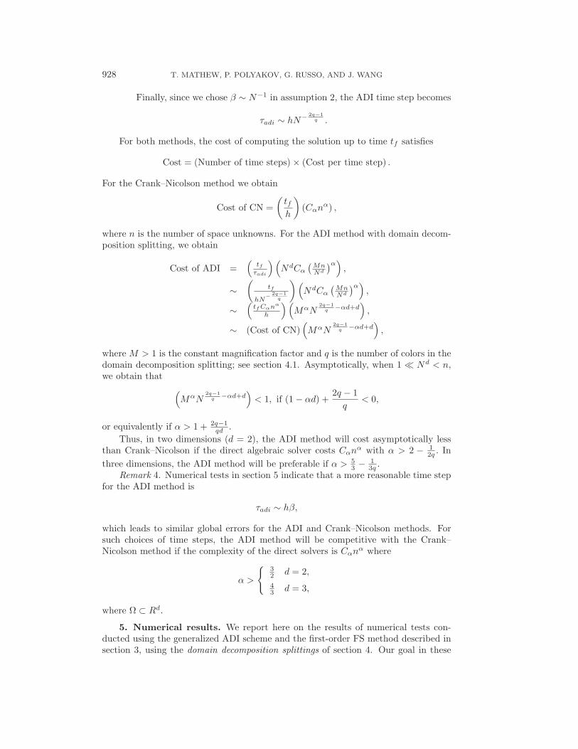
Finally, since we chose β ∼ N−1 in assumption 2, the ADI time step becomes

τadi ∼ hN− 2q−1q .

For both methods, the cost of computing the solution up to time tf satisfies

Cost = (Number of time steps) × (Cost per time step) .

For the Crank–Nicolson method we obtain

Cost of CN =(

tfh

)(Cαnα) ,

where n is the number of space unknowns. For the ADI method with domain decom-position splitting, we obtain

Cost of ADI =(

tf

τadi

)(NdCα

(MnNd

)α)

,

∼(

tf

hN− 2q−1

q

) (NdCα

(MnNd

)α)

,

∼(

tf Cαnα

h

)(MαN

2q−1q −αd+d

),

∼ (Cost of CN)(MαN

2q−1q −αd+d

),

where M > 1 is the constant magnification factor and q is the number of colors in thedomain decomposition splitting; see section 4.1. Asymptotically, when 1 � Nd < n,we obtain that (

MαN2q−1

q −αd+d)

< 1, if (1 − αd) +2q − 1

q< 0,

or equivalently if α > 1 + 2q−1qd .

Thus, in two dimensions (d = 2), the ADI method will cost asymptotically lessthan Crank–Nicolson if the direct algebraic solver costs Cαnα with α > 2 − 1

2q . Inthree dimensions, the ADI method will be preferable if α > 5

3 − 13q .

Remark 4. Numerical tests in section 5 indicate that a more reasonable time stepfor the ADI method is

τadi ∼ hβ,

which leads to similar global errors for the ADI and Crank–Nicolson methods. Forsuch choices of time steps, the ADI method will be competitive with the Crank–Nicolson method if the complexity of the direct solvers is Cαnα where

α >

{ 32 d = 2,

43 d = 3,

where Ω ⊂ Rd.

5. Numerical results. We report here on the results of numerical tests con-ducted using the generalized ADI scheme and the first-order FS method described insection 3, using the domain decomposition splittings of section 4. Our goal in these

DOMAIN DECOMPOSITION OPERATOR SPLITTINGS 929

TABLE 1Two nonoverlapping subdomains: Errors at time tf = 1; τcn = τadi = h.

h−1 17 33 49 65CN 0.0039 0.0010 4.5 × 10−4 2.5 × 10−4

ADI 0.0092 0.0024 0.0011 6.2 × 10−4

FS 0.39 0.19 0.12 0.090

tests was to compare the accuracies at a fixed time tf , say tf = 1, of the Crank–Nicolson solution when exact solvers are used with that of the ADI and first-orderFS solutions. Accordingly, we tabulate the global errors for the exact solver-basedCrank–Nicolson method and the ADI and first-order FS methods.

To enable computing the global error, we use the heat equation with a knownexact solution u(x, y, t) = et sin(πx) sin(πy) on the unit square Ω = [0, 1]2:⎧⎨

⎩ut = Δu + (1 + 2π2)et sin(πx) sin(πy) on Ω × [0, T ],

u(x, y, t = 0) = sin(πx) sin(πy) on Ω,u(x, y, t) = 0 on ∂Ω × [0, T ].

(24)

The standard five-point finite difference scheme was used to discretize in space on auniform grid of mesh size h. The Crank–Nicolson method was used to discretize intime with time steps τcn as indicated in the tables. In the tables, we tabulate thescaled Euclidean norm (scaled according to area) of the global error at time tf = 1 forthe Crank-Nicolson solution using exact solvers denoted by CN, and Crank–Nicolsonwith inexact ADI-based solvers denoted by ADI, and Crank–Nicolson with inexactfirst-order fractional step solvers denoted by FS.

Partitions of unity: The subdomains Ω∗k chosen in our experiments were rect-

angular. For the case of overlapping subregions, we constructed piecewise smoothpartitions of unity as follows. For a model rectangle Ω∗

k = [0, a] × [0, b] we defineωk(x, y) = sin(πx/a) sin(πy/b) inside Ω∗

k and zero outside it. Then, {χk(x, y)} isderived from {ωk(x, y)} as described in section 4.1.

Table 1 contains the results for the limiting case of zero overlap, i.e., β = 0.This case does not strictly fit in the theoretical framework developed in the pa-per. We consider two nonoverlapping subdomains Ω∗

1 = Ω1 = [0, 12 ] × [0, 1] and

Ω∗2 = Ω2 = [12 , 1] × [0, 1], and we define χi(x, y) = χΩi

(x, y), for i = 1, 2, i.e., thecharacteristic or indicator functions of the subdomains. In this case, the operatorsLk can only be defined weakly, in a variational sense. However, the finite differenceapproximations were well defined without additional modification since the grid wechose was aligned with the interface. Though the overlap β = 0, the numerical resultsindicate that the domain-decomposition-based ADI solution has, approximately, onlythrice as large errors compared to the solution of Crank–Nicolson with exact solvers.The FS solution, however, had about 100 times larger error than the CN solution.

Table 2 contains the results for two overlapping subdomains: Ω∗1 = [0, 3

4 ] × [0, 1]and Ω∗

2 = [14 , 1] × [0, 1]. In this case the overlap β = 1/4, and we note that thedomain-decomposition-based ADI solution has error very close to the CN solution(using exact solvers). The FS solution had approximately 50 times larger error thanthis CN solution.

Table 3 contains the results for the case of 16 overlapping subdomains, as shownin Figure 1. A 4 × 4 rectangular partition was first formed and each subrectanglewas enlarged to include overlap of β = 1/12 (1/3 of the subdomain width). Thesubdomains were grouped into q = 4 colors, and one of the four colored subregionsis shown in Figure 1. In solving (I + ατAk)w = z, parallelization is possible with

930 T. MATHEW, P. POLYAKOV, G. RUSSO, AND J. WANG

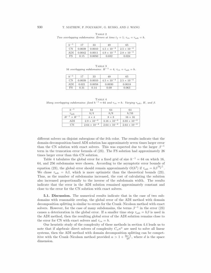
TABLE 2Two overlapping subdomains: Errors at time tf = 1; τcn = τadi = h.

h−1 17 33 49 65CN 0.0039 0.0010 4.5 × 10−4 2.5 × 10−4

ADI 0.0042 0.0011 4.9 × 10−4 2.8 × 10−4

FS 0.15 0.0050 0.032 0.024

TABLE 316 overlapping subdomains: H−1 = 4; τcn = τadi = h.

h−1 17 33 49 65CN 0.0039 0.0010 4.5 × 10−4 2.5 × 10−4

ADI 0.021 0.0058 0.0030 0.0018FS 0.31 0.14 0.09 0.063

TABLE 4Many overlapping subdomains: fixed h−1 = 64 and τcn = h. Varying τadi, H, and β.

h−1 64 64 64τadi h/4 h/8 h/16

H−1 × H−1 4 × 4 8 × 8 16 × 16ADI 2.9 × 10−4 3.16 × 10−4 3.03 × 10−4

CN 2.64 × 10−4 2.64 × 10−4 2.64 × 10−4

different solvers on disjoint subregions of the kth color. The results indicate that thedomain-decomposition-based ADI solution has approximately seven times larger errorthan the CN solution with exact solvers. This was expected due to the larger β−1

term in the truncation error formula of (23). The FS solution had approximately 26times larger error than this CN solution.

Table 4 tabulates the global error for a fixed grid of size h−1 = 64 on which 16,64, and 256 subdomains were chosen. According to the asymptotic error bounds ofequation (23), the global error should remain approximately O(h2) if τadi = hβ

2q−1q .

We chose τadi = hβ, which is more optimistic than the theoretical bounds (23).Thus, as the number of subdomains increased, the cost of calculating the solutionalso increased proportionally to the inverse of the subdomain width. The resultsindicate that the error in the ADI solution remained approximately constant andclose to the error for the CN solution with exact solvers.

5.1. Discussion. The numerical results indicate that in the case of two sub-domains with reasonable overlap, the global error of the ADI method with domaindecomposition splitting is similar to errors for the Crank–Nicolson method with exactsolvers. However, for the case of many subdomains, the terms β−1 in the error (23)causes a deterioration in the global error. If a smaller time step τadi = hβ is used inthe ADI method, then the resulting global error of the ADI solution remains close tothe error for CN with exact solvers and τcn = h.

Our heuristic study of the complexity of these methods in section 4.4 leads us tonote that if algebraic direct solvers of complexity Cαnα are used to solve all linearsystems, then the ADI method with domain decomposition splitting can be compet-itive with the Crank–Nicolson method provided α > 1 + 2q−1

qd , where d is the spacedimension.

DOMAIN DECOMPOSITION OPERATOR SPLITTINGS 931

Finally, we note that though the ADI method can become unstable, when q ≥ 3colors are used, such instability was not observed for the range of mesh, subdomain,and time step sizes used in our numerical experiments.

Acknowledgments. The authors thank Professors Max Dryja and Olof Wid-lund and the referees for helpful comments. They also express their gratitude toProfessor Patrick Le Tallec for a helpful suggestion regarding the ADI method dur-ing a presentation of this paper at the Seventh International Conference on DomainDecomposition Methods.

REFERENCES

[1] K. A. BAGRINOVSKII AND S. K. GODUNOV, Difference schemes for multidimensional problems,Dokl. Acad. Nauk USSR, 115 (1957), p. 431.

[2] H. BLUM, S. LISKY, AND R. RANNACHER, A domain splitting algorithm for parabolic problems,Computing: Archiv fur Informatik und Numerik, 49 (1992), pp. 11–23.

[3] F. A. BORNEMANN, An adaptive multilevel approach to parabolic equations: III. 2D errorestimation and multilevel preconditioning, Impact Comput. Sci. Engrg., 4 (1992), pp. 1–45.

[4] A. BRANDT, Guide to Multigrid Development, Lecture Notes in Math. 960, W. Hackbusch andU. Trottenberg, eds., Springer-Verlag, New York, 1981.

[5] X. C. CAI, Additive Schwarz algorithms for parabolic convection-diffusion equations, Numer.Math., 60 (1991), pp. 41–61.

[6] X. C. CAI, Multiplicative Schwarz methods for parabolic problems, SIAM J. Sci. Comput., 15(1994), pp. 587–603.

[7] T. CHAN AND T. MATHEW, Domain decomposition algorithms, Acta Numerica, 1994, pp. 61–143.

[8] T. F. CHAN AND J. ZOU, Optimal Domain Decomposition Algorithms for Non-symmetricProblems on Unstructured Meshes, Tech. report, Department of Mathematics, Universityof California, Los Angeles, CA, 1994.

[9] C. DAWSON, Q. DU, AND T. F. DUPONT, A finite difference domain decomposition algorithmfor numerical solution of the heat equation, Math. Comp., 57 (1991), pp. 63–71.

[10] J. DOUGLAS, JR., On the numerical integration of uxx + uyy = ut by implicit methods, J. Soc.Ind. Appl. Math., 3 (1955), pp. 42–65.

[11] J. DOUGLAS, JR., Alternating direction methods for three space variables, Numer. Math., 4(1961), pp. 41–63.

[12] J. DOUGLAS JR. AND J. E. GUNN, A general formulation of alternating direction method: PartI. Parabolic and hyperbolic problems, Numer. Math., 6 (1964), pp. 428–453.

[13] M. DRYJA, Substructuring methods for parabolic problems, in Fourth Internat. Symposium onDomain Decomposition Methods for Partial Differential Equations, R. Glowinski, Y. A.Kuznetsov, G. A. Meurant, J. Periaux, and O. Widlund, eds., SIAM, Philadelphia, PA,1991, pp. 264–271.

[14] R. GLOWINSKI AND P. L. TALLEC, Augmented Lagrangian and Operator-Splitting Methods inNonlinear Mechanics, SIAM Studies in Applied Mathematics 9, SIAM, Philadelphia, PA,1989.

[15] W. HACKBUSCH, Multi-grid Methods and Applications, Springer Ser. Comput. Math. 4,Springer Verlag, Berlin, Heidelberg, 1985.

[16] Y. A. KUZNETSOV, New algorithms for approximate realization of implicit difference schemes,Soviet J. Numer. Anal. Math. Modelling, 3 (1988), pp. 99–114.

[17] Y. A. KUZNETSOV, Overlapping domain decomposition methods for FE-problems with ellipticsingular perturbed operators, in Fourth Internat. Symposium on Domain DecompositionMethods for Partial Differential Equations, R. Glowinski, Y. A. Kuznetsov, G. A. Meurant,J. Periaux, and O. Widlund, eds., SIAM, Philadelphia, PA, 1991, pp. 223–241.

[18] Y. M. LAEVSKY, Direct Domain Decomposition Method for Solving Parabolic Equations, Tech.report preprint 940, Computing Center, Siberian Branch Academy of Sciences, Novosibirsk,Russia, 1992 (in Russian).

[19] Y. M. LAEVSKY, On the domain decomposition method for parabolic problems, Bulletin of theNovosibirsk Computing Center, 1 (1993), pp. 41–62.

[20] H. CHEN AND R. D. LAZAROV, Domain splitting algorithm for mixed finite element approxi-mations to parabolic problems, East-West J. Numer. Math., 4 (1996), pp. 121–135.

932 T. MATHEW, P. POLYAKOV, G. RUSSO, AND J. WANG

[21] G. A. MEURANT, Numerical experiments with a domain decomposition method for parabolicproblems on parallel computers, in Fourth Internat. Symposium on Domain DecompositionMethods for Partial Differential Equations, R. Glowinski, Y. A. Kuznetsov, G. A. Meurant,J. Periaux, and O. Widlund, eds., SIAM, Philadelphia, PA, 1991, pp. 394–408.

[22] D. W. PEACEMAN AND H. H. RACHFORD JR., The numerical solution of parabolic and ellipticdifferential equations, J. Soc. Ind. Appl. Math., 3 (1955), pp. 28–41.

[23] R. D. RICHTMYER AND K. W. MORTON, Difference Methods for Initial-value Problems, Wiley-Interscience, New York, 1967.

[24] G. STARKE, Alternating direction preconditioning for nonsymmetric systems of linear equa-tions, SIAM J. Sci. Comput., 15 (1994), pp. 369–384.

[25] S. STERNBERG, Lectures on Differential Geometry, Chelsea, New York, 1964.[26] G. STRANG, On the construction and comparison of difference schemes, SIAM J. Numer. Anal.,

5 (1968), pp. 506–517.[27] X. C. TAI, Domain decomposition for linear and non-linear elliptic problems via function

or space decomposition, in Domain Decomposition Methods in Scientific and EngineeringComputing, D. Keyes and J. Xu, eds., AMS, Providence, RI, 1994, pp. 355–360.

[28] P. N. VABISHCHEVICH, Parallel domain decomposition algorithms for time-dependent problemsof mathematical physics, in Advances in Numerical Methods and Applications, O(h3), I. T.Dimov, B. Sendov, and P. S. Vassilevski, eds., World Scientific, Singapore, 1994, pp. 293–299.

[29] P. N. VABISHCHEVICH AND P. MATUS, Difference schemes on grids locally refined in space aswell as in time, in Advances in Numerical Methods and Applications, O(h3), I. T. Dimov,B. Sendov, and P. S. Vassilevski, eds., World Scientific, Singapore, 1994, pp. 146–153.

[30] O. B. WIDLUND, On the rate of convergence of an alternating direction implicit method in anoncommutative case, Math. Comp., 20 (1966), pp. 500–515.

[31] O. B. WIDLUND, On difference methods for parabolic equations and alternating-direction-implicit methods for elliptic equations, IBM J. Research and Development, 11 (1967),pp. 239–243.

[32] O. B. WIDLUND, On the effects of scaling of the Peaceman-Rachford method, Math. Comp, 25(1971), pp. 33–41.

[33] J. XU, Iterative methods by space decomposition and subspace correction, SIAM Rev., 34 (1992),pp. 581–613.

[34] N. N. YANENKO, On weak approximation of systems of differential equations, Sibirsk. Mat.Zh., 5 (1964), p. 1430.