An iteration-by-subdomain overlapping Dirichlet/Robin domain decomposition method for...

Journal of Computational and Applied Mathematics 158 (2003) 243–276www.elsevier.com/locate/cam

An iteration-by-subdomain overlapping Dirichlet/Robin domaindecomposition method for advection–di+usion problems

Guillaume Houzeaux, Ramon Codina∗

Universitat Polit ecnica de Catalunya, Jordi Girona 1-3, Edi�ci C1, 08034 Barcelona, Spain

Received 6 February 2002; received in revised form 26 November 2002

Abstract

We present a new overlapping Dirichlet/Robin Domain Decomposition method. The method uses Dirichletand Robin transmission conditions on the interfaces of an overlapping partitioning of the computational domain.We derive interface equations to study the convergence of the method and show its properties through fournumerical examples. The mathematical framework is general and can be applied to derive overlapping versionsof all the classical nonoverlapping methods.c© 2003 Elsevier B.V. All rights reserved.

Keywords: Overlapping; Mixed domain decomposition method; Finite elements

1. Introduction

In this paper we present a domain decomposition (DD) method to solve scalar advection–di+usion–reaction (ADR) equations which falls into the category of iteration-by-subdomain DD methods.

Domain decomposition methods are usually divided into two families, namely overlapping andnonoverlapping methods. The former ones are based on the Schwarz method, >rst studied by Schwarzin 1869 and more recently returned to focus in [15]. At the di+erential level, this domain decompo-sition method uses alternatively the solution on one subdomain to update the Dirichlet data of theother. Although the Schwarz method presents a severe drawback, i.e., the dependence of the rate ofconvergence upon the overlapping length, as noted in [16]

[: : :] the Schwarz algorithm [: : :] presents some properties (like “robustness”, or indi+erence tothe type of equations considered...) which do not seem to be enjoyed by other methods.

∗ Corresponding author.E-mail address: [email protected] (R. Codina).

0377-0427/03/$ - see front matter c© 2003 Elsevier B.V. All rights reserved.doi:10.1016/S0377-0427(03)00447-3

mailto:[email protected]

244 G. Houzeaux, R. Codina / Journal of Computational and Applied Mathematics 158 (2003) 243–276

Contrary to the Schwarz method, nonoverlapping DD methods use necessarily two di+erent trans-mission conditions on the interface, in such a way that both the continuity of the unknown and its>rst derivatives are achieved on the interface (for ADR equations). The transmission conditions cancorrespond to the essential and natural boundary conditions of the weak form of the problem; how-ever, this is not a requirement. Four types of couplings are possible. The Dirichlet/Neumann methodwas introduced in [4] and presented in the >nite element context in [19] and extensively reviewedin [26]. Alonso et al. [2] developed a coercive Dirichlet/Robin method, called �-D/R, which uses theRobin transmission condition given by the natural condition of the weak formulation plus a constantto increase the coercivity of the associated preconditioner. The Robin/Robin method was >rst intro-duced in [17] for the Poisson equation as a generalization of the Schwarz method to nonoverlappingsubdomains. This method was reinterpreted within an augmented Lagrangian framework in [12].The freedom in choosing the coeJcients of the Robin condition, when one does not exactly usethe natural boundary condition of the weak form, has led to many formulations: see for example[23,18,24,2] for the coercive �-Robin/Robin method. The Robin/Neumann coupling is also a possiblechoice (see, e.g., [26]). Note that the case of the Neumann/Neumann method [5] is di+erent as itintroduces an additional system for each subdomain at the di+erential level. However, it leads at thealgebraic level to a preconditioned Richardson method, like the other methods introduced previously(see, e.g., [27,3,1]).

Some of these mixed methods present limitations, related to the fact that the boundary conditionsmust be imposed in accordance to the direction of the Kow when advection is dominant. Thisrequirement is at its turn closely related to the well-posedness of the local variational problems. Thiswas the argument for developing the so-called adaptive methods. Adaptive domain decompositionmethods take into account the direction of the Kow on the interface. The adaptive Dirichlet/Neumannmethod imposes a Dirichlet transmission condition at inKows and Neumann transmission conditionat outKows, the inKow on one side of the interface being the outKow on the other. See for example[6,7,11,30]. In [10], an iteration-by-subdomain DD method is devised to solve an advection–reactiontransport equation, where only Dirichlet data are prescribed on the inKow parts of the interface.

In the literature, all the mixed DD methods mentioned previously have been mainly studied inthe context of disjoint partitioning. However, there exists no particular reason for restricting theirapplication only to nonoverlapping subdomains. See for example [21,22,28]. This paper gives apossible line of study for the generalization of the mixed method to overlapping subdomains. Weexpect that the overlapping mixed DD methods will enjoy some properties of their disjoint brothersas well as some properties of the classical Schwarz method, as for example the dependence on theoverlapping length.

Our motivation to study these types of methods has been to maintain the implementation advan-tages of the Schwarz method when used together with a numerical approximation of the problem.The possibility to have some overlapping simpli>es enormously the discretization of the subdomains.However, very often this overlapping needs to be very small in practice, and thus the convergencerate of the Schwarz method becomes very small. Contrary to the Schwarz method, the limit case ofzero overlapping will be possible using the formulation proposed herein. We have chosen to study anoverlapping Dirichlet/Robin method, using the coercive bilinear form presented in [2] in the contextof the �-D/R and �-R/R methods. This simpli>es the analysis of the DD method as no assumptionhas to be made on the direction of the Kow and its amplitude on the interfaces of the overlappingsubdomains.

G. Houzeaux, R. Codina / Journal of Computational and Applied Mathematics 158 (2003) 243–276 245

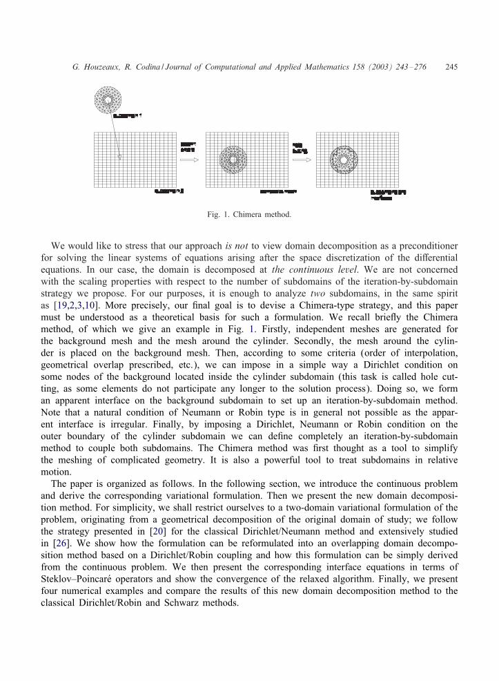
Fig. 1. Chimera method.

We would like to stress that our approach is not to view domain decomposition as a preconditionerfor solving the linear systems of equations arising after the space discretization of the di+erentialequations. In our case, the domain is decomposed at the continuous level. We are not concernedwith the scaling properties with respect to the number of subdomains of the iteration-by-subdomainstrategy we propose. For our purposes, it is enough to analyze two subdomains, in the same spiritas [19,2,3,10]. More precisely, our >nal goal is to devise a Chimera-type strategy, and this papermust be understood as a theoretical basis for such a formulation. We recall brieKy the Chimeramethod, of which we give an example in Fig. 1. Firstly, independent meshes are generated forthe background mesh and the mesh around the cylinder. Secondly, the mesh around the cylin-der is placed on the background mesh. Then, according to some criteria (order of interpolation,geometrical overlap prescribed, etc.), we can impose in a simple way a Dirichlet condition onsome nodes of the background located inside the cylinder subdomain (this task is called hole cut-ting, as some elements do not participate any longer to the solution process). Doing so, we forman apparent interface on the background subdomain to set up an iteration-by-subdomain method.Note that a natural condition of Neumann or Robin type is in general not possible as the appar-ent interface is irregular. Finally, by imposing a Dirichlet, Neumann or Robin condition on theouter boundary of the cylinder subdomain we can de>ne completely an iteration-by-subdomainmethod to couple both subdomains. The Chimera method was >rst thought as a tool to simplifythe meshing of complicated geometry. It is also a powerful tool to treat subdomains in relativemotion.

The paper is organized as follows. In the following section, we introduce the continuous problemand derive the corresponding variational formulation. Then we present the new domain decomposi-tion method. For simplicity, we shall restrict ourselves to a two-domain variational formulation of theproblem, originating from a geometrical decomposition of the original domain of study; we followthe strategy presented in [20] for the classical Dirichlet/Neumann method and extensively studiedin [26]. We show how the formulation can be reformulated into an overlapping domain decompo-sition method based on a Dirichlet/Robin coupling and how this formulation can be simply derivedfrom the continuous problem. We then present the corresponding interface equations in terms ofSteklov–PoincarLe operators and show the convergence of the relaxed algorithm. Finally, we presentfour numerical examples and compare the results of this new domain decomposition method to theclassical Dirichlet/Robin and Schwarz methods.


2. Problem statement

Let us consider the advection–di+usion–reaction problem of >nding u such that

Lu := −�Nu+∇ · (au) + �u= f in �;

u= 0 on 9�;(1)

where � is a d-dimensional domain (d=1; 2; 3) with boundary 9�, � is the di+usion constant of themedium, f is the force term, a is the advection >eld (not necessarily solenoidal) and � is a source(reaction) term.

We denote by (·; ·) the inner product in L2(�), and by V := H 10 (�) the space where u will be

sought. Likewise, we use the notation

〈·; ·〉! := 〈·; ·〉H−1=2(!)×H 1=200 (!) for ! d−1-dimensional;

〈·; ·〉! := 〈·; ·〉(H 1(!))′×H 1(!) for ! d-dimensional

for the duality pairings to be used. We endow H 1(�) with the usual scalar product (w; v)1;� =(w; v) + (∇w;∇v) and the associated norm ‖ · ‖1;�.

Let us consider our di+erential problem (1). We restrict ourselves to solutions in V . To guaranteeexistence, we take f∈ (H 1(�))′ and a; �;∇ · a∈L∞(�). By noting that∫

�va · ∇u d� =−

∫�ua · ∇v d� −

∫�uv∇ · a d� ∀u; v∈V;

we transform the convective term into a skew symmetric operator, and we can enunciate our problemas follows: >nd u∈V such that

a(u; v) = 〈f; v〉� ∀v∈V; (2)

where the bilinear form is

a(w; v) := �(∇w;∇v) + 12(a · ∇w; v)− 1

2 (w; a · ∇v) + (�0w; v)

with

�0 = � + 12 ∇ · a:

By applying Lax–Milgram lemma, it can be easily shown that if �0¿ 0 almost everywhere, Problem(2) has a unique solution.

3. Overlapping Dirichlet/Robin method

3.1. Domain partitioning and de�nitions

We perform a geometrical decomposition of the original domain � into three disjoint and con-nected subdomains �3, �4 and �5 such that

� = int(�3 ∪ �4 ∪ �5):


Fig. 2. Examples of decomposition of a domain � into two overlapping subdomains �1 and �2.

From this partition, we de>ne �1 and �2, as two overlapping subdomains:

�1 := int(�3 ∪ �4); �2 := int(�5 ∪ �4):

Finally, we de>ne �a as the part of 9�2 lying in �1, and �b as the part of 9�1 lying in �2, formallygiven by

�a := 9�2 ∩ �1; �b := 9�1 ∩ �2:

The geometrical nomenclature is shown in Fig. 2. �b and �a are the interfaces of the domaindecomposition method we now present. �4 is the overlap zone. In the following, index i or j referto a subdomain or an interface.

To state the variational formulation of the two-domain problem, we introduce the following de>-nitions:

(w; v)�i :=∫�i

wv d�;

ai(w; v) := �(∇w;∇v)�i +12(a · ∇w; v)�i − 1

2 (w; a · ∇v)�i + (�0w; v)�i ;

Vi := {v∈H 1(�i) | v|9�∩9�i= 0};

V 0i := H 1

0 (�i);

(3)

where i can be any of the >ve subdomains introduced previously, i.e., i = 1; 2; 3; 4 or 5.Let �0; i be the trace operators

�0; i :Vi → H 1=2(9�i); i = 1; 2; 3; 4; 5;

which are linear and continuous, like the trace operators Ta and Tb de>ned by

Ta :V → H 1=200 (�a); Tav= v|�a

;

Tb :V → H 1=200 (�b); Tbv= v|�b

:

We explicitly de>ne the trace spaces on �a and �b as �a := {�a ∈H 1=200 (�a)} and �b := {�b ∈

H 1=200 (�b)}, respectively.We also need to introduce some basic properties of the space we are working with; as many

constants are going to be introduced, we adopt a general nomenclature. We enunciate three inequal-ities (PoincarLe–Friedrichs, trace inequalities and an a priori estimate) that characterize the functionsbelonging to our working spaces, i.e., H 1(�) and H 1

0 (�). The domains of study are the originaldomain � and its >ve partitions �i, with i = 1; 2; 3; 4; 5. The PoincarLe–Friedrichs inequality reads

‖v‖20;�i6C�i‖∇v‖20;�i

∀v∈H 10 (�i); (4)


where C�i is a positive constant depending on the size of the domain �i. The space of applica-tion H 1

0 (�i) can be actually extended to any subspace of H 1(�i) for which the trace is speci>edsomewhere on 9�i.

The trace inequality is a direct consequence of the trace theorem; it states that there exists apositive constant C∗

i such that

‖v|9�i‖1=2;9�i 6C∗

i ‖v‖1;�i ∀v∈H 1(�i): (5)

Finally, the following a priori estimate for the solution v of homogeneous elliptic problems withDirichlet data holds (see, e.g., [9,25]):

‖v‖1;�i 6Ci‖v|9�i‖1=2;9�i ∀v∈H 1(�i): (6)

This establishes the continuous dependence of the solution on the boundary data and closes the listof properties we need.

3.2. Variational formulation

We propose to solve the following problem: >nd u1 ∈V1 and u2 ∈V2 such that

a1(u1; v1) = 〈f; v1〉�1 ∀v1 ∈V 01 ;

u1 = u2 on �b;

a2(u2; v2) = 〈f; v2〉�2 ∀v2 ∈V 02 ;

a3(u1; E3�a) + a2(u2; E2�a) = 〈f; E3�a〉�3 + 〈f; E2�a〉�2 ∀�a ∈�a;

(7)

where Ei denotes any possible extension operator from �a to H 1(�i), that is to say,

Ei :�a → H 1(�i); TaEi�a = �a ∀�a ∈�a:

Eqs. (7)1 and (7)3 are the equations for the unknown in subdomains �1 and �2 respectively. Eq.(7)2 is the condition that ensures continuity of the primary variable across �b, and levels the solutionin both subdomains. Finally, Eq. (7)4 is the equation for the primary variable on the interface �a.

Theorem 1. Problems (7) and (2) are equivalent.

Proof. We >rst show that the solution is the same in both subdomains inside the overlap zone�4, i.e., that the two transmission conditions on the interfaces are suJcient to uniquely de>ne thesolution. For any v4 ∈V 0

4 , construct

v1 =

{0 in �3;

v4 in �4

and v2 =

{v4 in �4;

0 in �5:

Clearly, v1 ∈V 01 and v2 ∈V 0

2 and therefore subtracting (7)1 and (7)3, we obtain

a4(u1 − u2; v4) = 0 ∀v4 ∈V 04

together with the condition u1 − u2 = 0 on �b, derived from (7)2. Now, we need to derive aboundary condition on �a in order to close the problem for the unknown u1 − u2. For any �a ∈�a


de>ne

v1 =

{E3�a in �3;

E4�a in �4:

Since v1 ∈V 01 , Eqs. (7)1 and (7)4 give

a2(u2; E2�a)− a4(u1; E4�a) = 〈f; E2�a〉�2 − 〈f; E4�a〉�4 ∀�a ∈�a: (8)

Now we de>ne for all �a ∈�a

v′2 =

{E4�a in �4;

0 in �5:

Eq. (8) can be rewritten as

a2(u2; E2�a − v′2) + a2(u2; v′2)− a4(u1; E4�a)

=〈f; E2� − v′2〉�2 + 〈f; v′2〉�2 − 〈f; E4�a〉�4 ∀�a ∈�a: (9)

According to the de>nition of v′2, (E2�a − v′2)∈V 02 and consequently, applying (7)3, we obtain

a2(u2; E2�a − v′2) = 〈f; E2� − v′2〉�2 :

Eq. (9) gives therefore

a4(u1 − u2; E4�a) = 0 ∀�a ∈�a:

As a result, the complete system of equations for w = u1 − u2 is

a4(w; v4) = 0 ∀v4 ∈V 04 ;

w = 0 on �b;

a4(w; E4�a) = 0 ∀�a ∈�a:

From the Lax–Milgram lemma, this problem has a unique solution w = 0; this implies that u1 = u2in �4.We now show that the solution of the original problem is also solution of the domain decompo-

sition problem. Let u be solution of Eq. (2), and de>ne ui = u|�ifor i = 1; 2. Clearly, ui ∈Vi and

therefore Eqs. (7)1, (7)2 and (7)3 are trivially satis>ed. Now for all �a ∈�a de>ne � as

�=

{E3�a in �3;

E2�a in �2:

We have that �∈V , which implies that

a(u; �) = 〈f; �〉�;and substituting the de>nition of � we recover Eq. (7)4.We now prove the reciprocal. Let

u=

{u1|�3

in �3;

u2 in �2:


We have shown that u1 = u2 in �4 and in particular that u1 = u2 on �a. This implies that u∈V and,as a result, we have

a(u; v) = a3(u1; v) + a2(u2; v) ∀v∈V: (10)

For each v∈V , set �a = Tav∈�a. Let us de>ne

�3 = v|�3− E3�a and �2 = v|�2

− E2�a;

and rewrite Eq. (10) as

a(u; v) = a3(u1; �3) + a3(u1; E3�a) + a2(u2; �2) + a2(u2; E2�a): (11)

By de>nition, �3 ∈V 03 . Let us now de>ne �1 as

�1 =

{�3 in �3;

0 in �4:

�1 ∈V 01 and therefore (7)1 implies that

a3(u1; �3) = 〈f; �3〉�3 :

Similarly, knowing also that �2 ∈V 02 , we can show that

a2(u2; �2) = 〈f; �2〉�2 ;

and from the latter two equations, Eq. (11) becomes

a(u; v) = 〈f; �3〉�3 + a3(u1; E3�a) + 〈f; �2〉�2 + a2(u2; E2�a) ∀�a ∈�a:

From Eq. (7)4, the last equation reads

a(u; v) = 〈f; �3〉�3 + 〈f; E3�a〉�3 + 〈f; �2〉�2 + 〈f; E2�a〉�2 ∀�a ∈�a;

which gives from the de>nitions of �3 and �2 yields,

a(u; v) = 〈f; v|�3〉�3 + 〈f; v|�2

〉�2 ;

= 〈f; v〉 ∀v∈V;

and hence the theorem follows.

Remark 2. The variational formulation given by Eqs. (7)1–4 provides a general setting for an over-lapping domain decomposition method. On the one hand, we have a Dirichlet condition on �b; onthe other hand, the transmission condition (7)4 on �a depends on the bilinear chosen to represent theoriginal di+erential operator in the weak formulation. For the particular case of the ADR problem,this condition can be written in the more familiar form presented next.

3.3. Alternative formulation

We develop an alternative formulation for the domain decomposition method given by Eqs. (7)1–4.


Lemma 3. The solution of the domain decomposition problem satis�es

�9u19n2

− 12(a · n2)u1 = �

9u29n2

− 12(a · n2)u2 on �a;

where 9(·)=9n2 = n2 · ∇(·), n2 being the exterior normal to �2 on �a.

Proof. According to Green’s formula, for all �a ∈�a we have

a3(u1; E3�a) =−⟨�9u19n2

− 12(a · n2)u1; �a

⟩�a

+ 〈Lu1; E3�a〉�3 ; (12)

a2(u2; E2�a) =⟨�9u29n2

− 12(a · n2)u2; �a

⟩�a

+ 〈Lu2; E2�a〉�2 : (13)

In addition, from Eqs. (7)1 and (7)3, we have that

Lu1 = f in �1 and Lu2 = f in �2;

in the sense of distributions. As a result, Eqs. (12) and (13) become

a3(u1; E3�a) =−⟨�9u19n2

− 12(a · n2)u1; �a

⟩�a

+ 〈f; E3�a〉�3 ;

a2(u2; E2�a) =⟨�9u29n2

− 12(a · n2)u2; �a

⟩�a

+ 〈f; E2�a〉�2 :

(14)

Adding up these two equations, and substituting the result into Eq. (7)4, we >nd⟨−�9u19n2

+12(a · n2)u1 + �

9u29n2

− 12(a · n2)u2; �a

⟩�a

= 0 ∀�a ∈�a;

and thus the lemma holds.

Theorem 4. System of Eqs. (7)1–4 can be reformulated as follows: �nd u1 ∈V1 and u2 ∈V2 suchthat

a1(u1; v1) = 〈f; v1〉�1 ∀v1 ∈V 01 ;

u1 = u2 on �b;

a2(u2; v′2) = 〈f; v′2〉�2 +⟨�9u19n2

− 12(a · n2)u1; v′2

⟩�a

∀v′2 ∈V2:

(15)

Proof. We >rst substitute Eq. (14) into Eq. (7)4, and add the result to Eq. (7)3:

a2(u2; v2 + E2�a) =⟨�9u19n2

− 12(a · n2)u1; �a

⟩�a

+ 〈f; v2 + E2�a〉�2 ∀v2 ∈V 02 ; �a ∈�a:

Let us de>ne v′2 = v2 + E2�a. Clearly, v′2 ∈V2 and �a = Tav′2; consequently, the last equation isequivalent to

a2(u2; v′2) =⟨�9u19n2

− 12(a · n2)u1; v′2

⟩�a

+ 〈f; v′2〉�2 ∀v′2 ∈V2:


The proof is completed by substituting Eqs. (7)3 and (7)4 of the system of equations (7)1–4 by thelatter equation.

The interpretation of the domain decomposition method now appears clearly. A Dirichlet problemis solved in �1 using as Dirichlet data on the interface �b the solution in �2, whereas a mixedDirichlet/Robin problem is solved in �2 using as Robin data on �a the solution in �1. This formu-lation justi>es the name overlapping Dirichlet/Robin method to designate this domain decompositionmethod.

Remark 5. The system of equations (15)1–3 could have been derived directly from the followingDD problem applied at the di+erential level:

Lu1 = f in �1;

u1 = 0 on 9�1 ∩ 9�;u1 = u2 on �b;

Lu2 = f in �2;

u2 = 0 on 9�2 ∩ 9�;

�9u29n2

− 12(a · n2)u2 = �

9u19n2

− 12(a · n2)u1 on �a:

(16)

The interface conditions on �a and �b are usually referred to as matching conditions or transmissionconditions. The >rst one is of Dirichlet type while the second one is of Robin type. At the variationallevel, we have just shown they correspond to essential and natural boundary conditions.

3.4. Interface equations

A convenient way to study DD methods is to derive equations for the interface unknown(s). Todo so, the problem is >rst rewritten into two purely Dirichlet problems for which the Dirichlet dataare the unknowns on the interfaces. For the sake of clarity, the derivation of the interface equationsis carried out at the di+erential level, starting from Eqs. (16)1–6. The problems to consider are:

Lw1 = f in �1; Lw2 = f in �2;

w1 = 0 on 9�1 ∩ 9�; w2 = 0 on 9�2 ∩ 9�;w1 = �b on �b; w2 = �a on �a:

(17)

Now let us decompose w1 and w2 into L-homogeneous and Dirichlet-homogeneous parts,

w1 = u01 + u∗1 ; w2 = u02 + u∗2 ;

where the L-homogeneous parts u01 and u02 are the solutions of the following systems:

Lu01 = 0 in �1; Lu02 = 0 in �2;

u01 = 0 on 9�1 ∩ 9�; u02 = 0 on 9�2 ∩ 9�;u01 = �b on �b; u02 = �a on �a

(18)


and the Dirichlet-homogeneous parts u∗1 and u∗2 are the solutions of the following systems:

Lu∗i = f in �i;

u∗i = 0 on 9�i

(19)

for i = 1; 2. We refer to u01 as the L-homogeneous extension of �b into �1, and we denote it byL1�b. Similarly, we call u02 the L-homogeneous extension of �a into �2, and we denote it by L2�a.In the case when L = −�, L is called the harmonic extension and is usually denoted by H . TheDirichlet-homogeneous parts u∗1 and u∗2 are rewritten as G1f and G2f, respectively.

Comparing systems (17) with system (16), we have that wi = ui for i = 1; 2 if and only if thefollowing two conditions are satis>ed:

�9w2

9n2− 1

2(a · n2)w2 = �

9w1

9n2− 1

2(a · n2)w1 on �a;

w1 = w2 on �b: (20)

Using the previous de>nitions, conditions (20) can be rewritten as

�9L2�a9n2

− 12(a · n2)L2�a

=�9L1�b9n2

− 12(a · n2)L1�b + �

9G1f9n2

− 12(a · n2)G1f − �

9G2f9n2

+12(a · n2)G2f on �a;

�b = TbL2�a + TbG2f on �b:

Let us clean up this system by introducing some de>nitions. In the >rst equation, we recognize theSteklov–PoincarLe operator S2 associated to subdomain �2, and de>ned as

S2 :�a → H−1=2(�a);

S2�a := �9L2�a9n2

− 12(a · n2)L2�a (evaluated on �a):

Note that L2�a = �a on �a. We de>ne S̃b, a Steklov–PoincarLe-like operator acting on �b, as

S̃b :�b → H−1=2(�a);

S̃b�b := −�9L1�b9n2

+12(a · n2)L1�b (evaluated on �a):

We also de>ne T̃ b, the trace on �b of the L-extension of �a into �2:

T̃ b :�a → �b;

T̃ b�a := TbL2�a:

Finally, and ′ are de>ned as follows:

= �9G1f9n2

− 12(a · n2)G1f − �

9G2f9n2

+12(a · n2)G2f;

′ = TbG2f;


where we have ∈H−1=2(�a) and ′ ∈�b. Owing to the previous de>nitions, the system of twoequations for the interface unknowns reads

S2�a =−S̃b�b + in H−1=2(�a);

�b = T̃ b�a + ′ in �b: (21)

Let us introduce now the operator

S̃1 :�a → H−1=2(�a);

S̃1�a := S̃bT̃ b�a

and de>ne S as

S = S̃1 + S2:

After substituting �b given by Eq. (21)2 into Eq. (21)1, we >nally obtain the following system ofequations for the interface unknowns:

S�a = − S̃b ′ in H−1=2(�a);

�b = T̃ b�a + ′ in �b: (22)

Once �a and �b are obtained, we can solve the two Dirichlet problems (18) to obtain the L-homogeneous parts u01 and u02. The Dirichlet-homogeneous parts u∗1 and u∗2 are obtained by solv-ing Eqs. (19) for i=1; 2. Hence, the solutions u1 and u2 are calculated by adding up their respectiveL and Dirichlet-homogeneous contributions. Eq. (22)1 should formally be understood in a weaksense, i.e.,

〈(S2 + S̃1)�a; �a〉�a = 〈 − S̃b ′; �a〉�a ∀�a ∈�a: (23)

Lemma 6. The variational counterpart of the Steklov–Poincar>e operators are

〈S̃1�a; �a〉�a = a3(L1T̃ b�a; E3�a); (24)

〈S2�a; �a〉�a = a2(L2�a; E2�a) ∀�a ∈�a (25)

for any extension operators E2 and E3.

Proof. The lemma follows from the de>nitions of S̃1 and S2 and Green’s formula.

We can also show that the two right hand-side terms of Eq. (22)1 satisfy

〈 ; �a〉�a = 〈f; E2�a〉�2 − a2(G2f; E2�a) + 〈f; E3�a〉�3 − a3(G1f; E3�a);

〈S̃b ′; �a〉�a = a3(L1TbG2f; E3�a) ∀�a ∈�a

for any extension operators E2 and E3. This completes the de>nition of the variational form of Eq.(22)1, i.e.,

a2(L2�a; E2�a) + a3(L1T̃b�a; E3�a)

=〈f; E2�a〉�2−a2(G2f; E2�a)+〈f; E3�a〉�3− a3(G1f; E3�a)−a3(L1TbG2f; E3�a) ∀�a ∈�a:


Remark 7. Eq. (23) can be also obtained by formulating problems (17) in a variational form.

Let us go back to system (22). We >rst state some useful properties of operators S2 and S̃1.

Lemma 8. S2 is both continuous and coercive and S̃1 is continuous and nonnegative.

Proof. We have shown that Eqs. (25) and (24) hold for any extension operators E2 and E1.This leaves us the choice to >nd appropriate expressions for S2 and S̃1 to facilitate their analysis.A straightforward choice consists of taking E2 =L2, and E1 =L1T̃ b. Thus, we have

〈S2�a; �a〉�a = a2(L2�a;L2�a);

〈S̃1�a; �a〉�a = a3(L1T̃ b�a;L1T̃ b�a) ∀�a ∈�a:

We >rst show that S2 is both continuous and coercive. Using the de>nition of a2 given by Eq. (3)and applying the Cauchy–Schwartz inequality, we obtain

〈S2!a; �a〉�a 6 "�2‖L2!a‖1;�2‖L2�a‖1;�2 ∀!a; �a ∈�a; (26)

where "�2 = �+ ‖a‖∞;�2 + ‖�0‖∞;�2 . According to the a priori estimate given by Eq. (6), we havethat ‖L2�a‖1;�2 6C2‖�a‖1=2; (�a) for �a ∈�a, and therefore Eq. (26) gives

〈S2!a; �a〉�a 6MS2‖!a‖1=2;�a‖�a‖1=2;�a ∀!a; �a ∈�a; (27)

which states that S2 is continuous, with MS2 = "�2C22 the continuity constant. We now show the co-

ercivity of S2. Owing to the skew-symmetry of the convective term of a2, for any �a ∈�a we have

〈S2�a; �a〉�a

=a2(L2�a;L2�a) = � ‖∇L2�a‖20;2 +∫�2

�0(L2�a)2 d�

¿ �‖∇L2�a‖20;�2(�0¿ 0 almost everywhere): (28)

From the trace inequality (see Eq. (5)), we know that there exists a constant C∗2 ¿ 0 such that

‖L2�a|9�2‖1=2;9�2 6C∗

2 ‖L2�a‖1;�2 ∀�a ∈�a;

Using the PoincarLe–Friedrichs inequality (4), Eq. (28) yields

〈S2�a; �a〉¿NS2‖�a‖21=2;�a∀�a ∈�a; (29)

where NS2 := �=(C2�2

+ 1)(C∗2 )

2 is the coercivity constant.Let us >nally prove the continuity and nonnegativeness of S̃1. Applying the Cauchy–Schwarz

inequality to Eq. (24), we obtain

〈S̃1!a; �a〉�a 6 "�3‖L1TbL2!a‖1;�3‖L1TbL2�a‖1;�3

6 "�3‖L1TbL2!a‖1;�1‖L1TbL2�a‖1;�1 (�3 ⊂ �1)

for any !a; �a ∈�a and where "�3 = � + ‖a‖∞;�3 + ‖�0‖∞;�3 . From the a priori estimate given byEq. (6), we have that

〈S̃1!a; �a〉�a

6 "�3C21‖TbL2!a‖1=2;9�1‖TbL2�a‖1=2;9�1


="�3C21‖TbL2!a‖1=2;�b‖TbL2�a‖1=2;�b

="�3C21‖�0;5L2!a‖1=2;9�5‖�0;5L2�a‖1=2;9�5

6 "�3C21C

∗25 ‖L2!a‖1;�5‖L2�a‖1;�5 (trace inequality (5))

6 "�3C21C

∗25 ‖L2!a‖1;�2‖L2�a‖1;�2 (�5 ⊂ �2)

6 "�3C21C

∗25 C2

2‖!a‖1=2;9�2‖�a‖1=2;9�2 (a priori estimate (6))

=MS̃1‖!a‖1=2;�a‖�a‖1=2;�a ; (30)

which proves the continuity of S̃1. Finally, owing to the skew-symmetry of a1, for any �a ∈�a wehave

〈S̃1�a; �a〉�a = a1(L1T̃ b�a;L1T̃ b�a)

= � ‖∇L1T̃ b�a‖20;2 +∫�3

�0(L1T̃ b�a)2 d�

¿ 0 (�0¿ 0 almost everywhere);

and the lemma holds.

The following result is a direct consequence of the previous properties:

Theorem 9. System (22) has a unique solution {�a; �b}.

Proof. We >rst prove that S is invertible, showing that it is both continuous and coercive. We have

〈S!a; �a〉�a = 〈S̃1!a; �a〉�a + 〈S2!a; �a〉�a ∀!a; �a ∈�a:

Therefore, the continuity of S follows from that of S2 and S̃1, i.e.,

〈S!a; �a〉6MS‖!a‖1=2;�a‖�a‖1=2;�a ∀!a; �a ∈�a

with continuity constant MS given by MS=MS̃1+MS2 , where MS̃1 and MS2 are the continuity constantsof S̃1 and S2 introduced in Eqs. (30) and (27), respectively.We now show the coercivity of S without trying to obtain sharp estimates. We have already

shown the coercivity of S2 and the nonnegativeness of S̃1. Therefore,

〈S�a; �a〉�a

=〈S2�a; �a〉�a + 〈S̃1�a; �a〉�a

¿ 〈S2�a; �a〉�a ¿NS‖�a‖21=2;�a∀�a ∈�a;

where NS =NS2 . Thus, S is a continuous and coercive operator. According to Lax–Milgram Lemma,it is invertible and therefore Eq. (22)1 has a unique solution �a. The existence and uniqueness of �bfollows from that of �a, by applying Eq. (22)2. Remember that we have

�b = T̃ bL2�a + ′:


L2�a is the unique solution of problem (18)2. Since the trace operator Tb is well de>ned, fromH 1(�2) onto �b, we have that �b exists and is unique. Inverting S in Eq. (22)1, we >nd that

�a = S−1( − S̃b ′) in �a;

�b = T̃ bS−1( − S̃b ′) + ′ in �b;

are the solutions of our interface problem.

4. Iterative scheme

4.1. Relaxed sequential algorithm

In this section, we derive an iterative procedure to solve the domain decomposition problem (7).The sequential version of the iterative overlapping D/R algorithm is de>ned as follows. Given aninitial guess u02 on �b, for each k¿ 0, >nd uk+1

1 ∈V1 and uk+12 ∈V2 such that

a1(uk+11 ; v1) = 〈f; v1〉�1 ∀v1 ∈V 0

1 ;

uk+11 = uk2 on �b;

a2(uk+12 ; v2) = 〈f; v2〉�2 ∀v2 ∈V 0

2 ;

a2(uk+12 ; E2�a) =−a3(uk+1

1 ; E3�a) + 〈f; E3�a〉�3 + 〈f; E2�a〉�2 ∀�a ∈�a;

(31)

for any extension operators E3 and E2. If this algorithm converges, the solutions on both subdomainssatisfy Eqs. (7)1–4. The corresponding algorithm for the di+erential problem given by Eqs. (16)1–6is straightforward and reads: given an initial guess u02 on �b, for each k¿ 0, >nd uk+1

1 and uk+12

such that

Luk+11 = f in �1;

uk+11 = 0 on 9�1 \ �b;

uk+11 = uk2 on �b;

Luk+12 = f in �2;

uk+12 = 0 on 9�2 \ �a;

�9uk+1

2

9n2− 1

2(a · n2)uk+1

2 = �9uk+1

1

9n2− 1

2(a · n2)uk+1

1 on �a:

(32)

If this algorithm converges, the solutions on both subdomains satisfy Eqs. (16)1–6. For the sake ofclarity, we have omitted the relaxation of the transmission conditions; for example, the Dirichletcondition (32)2 could be replaced by

uk+11 = 'uk2 + (1− ')uk1;

where '¿ 0 is the relaxation parameter.


Fig. 3. Relaxed sequential algorithms. (Left) D'=R method. (Right) D=R' method.

We now investigate the interface iterates produced by this relaxed iterative procedure. The set ofequations for the wi’s is the following:

Lwk+11 = f in �1; Lwk+1

2 = f in �2;

wk+11 = 0 on 9�1 ∩ 9�; wk+1

2 = 0 on 9�2 ∩ 9�;wk+11 = �kb on �b; wk+1

2 = �k+1a on �a:

The choice of taking as Dirichlet conditions �b at iteration k for wk+11 , and �a at iteration k + 1 for

wk+12 is arbitrary. According to this choice, we can set

wk+11 =L1�kb + G1f; wk+1

2 =L2�k+1a + G2f:

We have that wki = uki for i = 1; 2 if and only if the wk

i ’s satisfy the transmission conditions (32)3and (32)6. By noting that the Dirichlet-homogeneous solutions G1f and G2f do not change alongthe iterative process, the Dirichlet-relaxed iterative scheme, denoted D'=R, is given for any k¿ 0by

S2�k+1a =−S̃b�kb + ;

�k+1b = '(T̃ b�k+1

a + ′) + (1− ')�kb:(33)

The Robin transmission condition can be also relaxed by replacing Eq. (32)6 by

�9uk+1

2

9n2− 1

2(a · n2)uk+1

2 = '[�9uk+1

1

9n2− 1

2(a · n2)uk+1

1

]+ (1− ')

[�9uk29n2

− 12(a · n2)uk2

]:

In terms of the interface unknowns, the Robin-relaxed iterative scheme, denoted D=R', produces thefollowing iterates for any k¿ 0:

S2�k+1a = '(−S̃b�kb + ) + (1− ')S2�ka;

�k+1b = T̃ b�k+1

a + ′:(34)

The dependence of �k+1a and �k+1

b on the values at previous iterations, given two initial values �0aand �0b, is sketched in Fig. 3; note that the value of �0a is only needed when using the D=R' method.The continuity and coercivity of S2 has been proven in last section. According to Lax–Milgram

Lemma, S2 is invertible. We can therefore reformulate the system for the interface unknowns (21)as follows:

Qa�a = a;

Qb�b = b;(35)


where we have de>ned Qa, Qb, a and b by

Qa = Ia + S−12 S̃bT̃ b = Ia + S−1

2 S̃1;

Qb = Ib + T̃ bS−12 S̃b;

a = S−12 − S−1

2 S̃b ′;

b = T̃ bS−12 + ′

and where Ia is the identity on �a and Ib is the identity on �b. By solving the Dirichlet- andRobin-relaxed systems for �k+1

a and �k+1b , we can show that both schemes lead to the same following

iterates for any k¿ 1:

�k+1a = '( a − Qa�ka) + �ka;

�k+1b = '( b − Qb�kb) + �kb:

(36)

We recognize here two stationary Richardson procedures for solving Eqs. (35)1 and (35)2. TheRichardson procedure for solving �a is similar to that produced by the classical Dirichlet/Neumannmethod; in fact, we obtain the following equivalent iterate:

�k+1a = 'S−1

2 [( − S̃b ′)− S�ka] + �ka;

which is a preconditioned Richardson method for solving Eq. (22)1, using S2 as preconditionerfor S.

Remark 10. As pointed out above, the Richardson procedures (36) are valid only for k¿ 1. TheD'=R and D=R' methods are therefore not completely equivalent, as the >rst iterative values �1a and�1b may di+er, even if �0a and �0b are chosen to be equal. Therefore, even though they have the samebehavior (given by Eq. (36)) they may yield di+erent values of the iterates �ka; �kb, k = 1; 2; 3; : : : :

4.2. Convergence

This section studies the convergence of the D'=R and D=R' iterative schemes given by Eqs.(32)1–6 at the di+erential level, or (31)1–4 at the variational level. Rather than directly studying thewhole system of equations for u1 and u2, we base our analysis on the equivalent interface equationssystems, i.e., Eqs. (33)1−2 for the D'=R method and Eqs. (34)1–2 for the D=R' method. The resultwe can prove is

Theorem 11. Assume that � is large enough so that

"∗ := 2NS2 − 2‖a‖∞;�aC22

MS̃1 +MS2

NS2¿ 0; (37)

where the constants NS2 , MS̃1 and MS2 have been introduced in Eqs. (29), (30) and (27), respectively.Then, there exists 'max such that for any given �0a ∈�a and �0b ∈�b and for all '∈ (0; 'max), thesequences {�ka} and {�kb} given by (36) converge in �a and �b, respectively. The upper bound ofthe relaxation parameter 'max can be estimated by

'max ="∗N 2

S2

MS2(MS̃1 +MS2)2: (38)


More precisely, convergence is linear, the convergence factor being K' ¡ 1 de�ned in the proofbelow.

Proof. The proof is split into two steps. We >rst show the Richardson procedure for the sequence{�ka} given by Eq. (36)1 converges. The proof is based on the abstract Theorem 3.1 of [2], orTheorem 4.2.2 of [26]. Secondly, we show that if the sequence {�ka} converges, then {�kb} does aswell.

Let us start with the >rst step and de>ne Ra the Richardson iteration operator as

Ra :�a → H−1=2(�a);

Ra�a := (Ia − 'Qa)�a = (Ia − 'S−12 S)�a:

If we de>ne eka = �ka − �a as the error with respect to �a at iteration k, �a being solution of problem(35)1, the error equation reads

ek+1a = Raeka:

The Richardson procedure (36)1 is therefore convergent if the operator Ra is a contraction withrespect to some norm. Let us introduce the following application:

(·; ·)S2 :�a × �a → R;

(!a; �a)S2 :=12(〈S2!a; �a〉�a + 〈S2�a; !a〉�a):

It is easy to check that this application is a scalar product, and that it induces the following S2-norm:

‖�a‖S2 := 〈S2�a; �a〉1=2�a;

which, owing to both the coercivity and continuity of S2, is equivalent to the natural norm on �a,i.e.,

N 1=2S2 ‖�a‖1=2;�a 6 ‖�a‖S2 6M 1=2

S2 ‖�a‖1=2;�a ∀�a ∈�a: (39)

By de>nition we have

‖Ra�a‖2S2 = ‖�a‖2S2 + ' 2〈S�a; S−12 S�a〉�a − '(〈S2�a; S−1

2 S�a〉�a + 〈S�a; �a〉�a): (40)

Using the same strategy as in [26], it can be checked that

〈S2�a; S−12 S�a〉�a + 〈S�a; �a〉�a ¿ "∗‖�a‖21=2;�a

∀�a ∈�a

with "∗ de>ned in Eq. (37). Since the norm of S−12 is 1=NS2 , and owing to the continuity of S2 and

S̃1 and to the assumption of the theorem, Eq. (40) yields

‖Ra�a‖2S2 6K'‖�a‖2S2with K' given by

K' = 1 + ' 2 (MS2 +MS̃1)2

N 2S2

− '"∗

MS2:


The Richardson procedure is a contraction in the S2-norm if K' ¡ 1, i.e., if 0¡'¡'max, with 'maxgiven by Eq. (38).

Let us now go on to the second step of the proof, i.e., the convergence of the sequence {�ka}implies that of the sequence {�kb}. Although the Dirichlet and Robin-relaxed methods lead to the sameRichardson procedure for �b (Eq. (36)2) for k¿ 1, we have to treat their convergence separately.We de>ne ekb = �kb − �b. Since the converged solution satis>es �b = T̃ b�a + ′, Eq. (34)2 for theRobin-relaxed scheme gives for any k¿ 1,

ekb = T̃ beka:

Therefore, we have

‖ekb‖1=2;�b

=‖TbL2eka‖1=2;�b

6C∗2 ‖L2eka‖1;�2 (trace inequality (5))

6C∗2C2‖eka‖1=2;�a (a priori estimate (6))

6C∗2C2

N 1=2S2

‖eka‖S2 (norm equivalence (39))

6Kk'C∗2C2

N 1=2S2

‖e0a‖1=2;�a ;

which shows that the sequence {�kb} converges whenever K' ¡ 1.Now we study the convergence of the Dirichlet-relaxed algorithm (for ' �= 1). From Eq. (33)2,

we have that, for any k¿ 1,

ekb = 'T̃ beka + (1− ')ek−1b :

According to this equation, we can generate the following sequence:

ekb = ' T̃ beka + (1− ') ek−1b ;

(1− ') ek−1b = '(1− ') T̃ bek−1

a + (1− ')2 ek−2b ;

(1− ')2 ek−2b = '(1− ')2 T̃ bek−2

a + (1− ')3 ek−3b ;

......

(1− ')k−2 e2b = '(1− ')k−2 T̃ be2a + (1− ')k−1 e1b;

(1− ')k−1 e1b = '(1− ')k−1 T̃ be1a + (1− ')k e0b:

Adding up all the terms, we >nd the following equality:

ekb = (1− ')ke0b + '(1− ')kk∑

n=1

(1− ')−nT̃ beka;


which gives

‖ekb‖1=2;�b 6 |1− '|k‖e0b‖1=2;�b + '|1− '|kk∑

n=1

|1− '|−n‖TbL2ena‖1=2;�b

6 |1− '|k ‖e0b‖1=2;�b +'K'

|1− '|k−1 C∗2C2

N 1=2S2

‖e1a‖S2k∑

n=1

(K'

|1− '|)n

:

The geometric progression is

k∑n=1

(K'

|1− '|)n

=

12 k(k + 1) if K' = |1− '|;

K'

|1− '|k|1− '|k − Kk

'

|1− '| − K'otherwise;

and thus we >nd the following two expressions for the norm of the error:

‖ekb‖1=2;�b 6

|1− '|k(‖e0b‖1=2;�b +

12k(k + 1)'

C∗2C2

N 1=2S2

‖e0a‖S2)

if K' = |1− '|;

|1− '|k‖e0b‖1=2;�b + '|1− '|k − Kk

'

|1− '| − K'

C∗2C2

N 1=2S2

‖e0a‖S2 otherwise:

Owing to these inequalities and since '¡ 2 (see Eqs. (37)–(38)), we conclude that if K' ¡ 1 thesequence {�kb} converges.

Note that once �a=limk→∞ �ka and �b=limk→∞ �kb are found, the solutions in �1 and �2 are ob-tained by solving the two Dirichlet problems given by Eqs. (17). As a consequence, the convergencesof sequences {�ka} and {�kb} imply the convergence of the whole algorithm.

Remark 12. This result carries over to the discrete variational problems provided the stability andcontinuity properties of the continuous case are inherited. In particular, the rate of convergence willbe independent of the number of degrees of freedom.

5. Numerical examples

We present four numerical examples to test the overlapping D/R method in the di+usion as wellas in the advection dominated limits. We apply the DD method to the discrete problem, rather to thecontinuous one considered up to now. However, the decomposition given by Eq. (7) and the resultswe have proven related to it apply also to the discrete (>nite-dimensional) setting resulting froma �nite element discretization, that is what we consider in what follows. In particular, in all thecases we consider a >nite element partition of the computational domain made of piecewise bilinearquadrilateral elements.


Fig. 4. Computational domain and boundary conditions.

5.1. Skew advection

Through this example, which was used as a >rst test case of the classical �-D/R method in [2],we want to compare the disjoint and overlapping versions of the D/R method for a skew advection>eld. As an additional indication when using overlapping grids, we will systematically give theresults of the Schwarz method (D/D) for overlapping subdomains, and that of the adaptive D/Nmethod (A-D/N) for both disjoint and overlapping subdomains. The overlapping version of theA-D/N method uses a Neumann interface at outKow and a Dirichlet interface at inKow, as in theclassical disjoint case. We propose to solve the equation

−�Nu+ a · ∇u= f in � = (0; 1)× (0; 1)

with a skew advection >eld a = [1; 1]t, and look for the exact solution u= u(x; y) = x + 5y, whichbelongs to the >nite element space of work. According to this choice, we impose f = 6, and exactDirichlet conditions on the boundary; see Fig. 4.

We de>ne three di+erent meshes, with h=1=10, 1=20 and 1=40. In addition, we de>ne three di+erentpartitionings. The splitting of the two subdomains is always performed vertically and symmetricallywith respect to the line x=0:5. The >rst partition splits � into two disjoint subdomains, the secondinto two overlapping subdomains with horizontal overlapping length 1= 0:2, and the third one with1 = 0:4. As for the numerical strategy, we use the variational subgrid scale model (indispensablefor small �), as described in [8]. In order to introduce as few extrinsic errors to the DD methodsthemselves as possible, all the matrices involved in the Schur complement system are inverted usinga direct solver. When considering disjoint subdomains, the convergence criterion is

100‖uk+1

�a− uk�a

‖2‖uk�a

‖26 10−10;

while for overlapping subdomains it is given by

100‖uk+1

�a− uk�a

‖2 + ‖uk+1�b

− uk�b‖2

‖uk�a‖2 + ‖uk�b

‖26 10−10;


Table 1Number of iterations (' = 0:5, 1= 0)

� \ h D/R A-D/N

1=10 1=20 1=40 1=10 1=20 1=40

101 2 2 2 8 8 8100 5 4 2 15 15 1510−1 7 6 5 31 31 3110−2 8 8 7 39 39 3910−3 8 8 8 40 40 4010−4 9 8 8 41 41 4110−5 9 8 8 41 41 41

Table 2'opt and number of iterations (1= 0)

� D/R A-D/N

'opt No. 'opt No.

101 0.50 2 0.50 8100 0.50 4 0.54 1110−1 0.50 6 0.65 1910−2 0.50 8 0.81 1710−3 0.50 8 0.90 1710−4 0.50 9 0.93 1810−5 0.50 9 0.93 18

where uk�aand uk�b

are the arrays of nodal unknowns corresponding to the nodes on the interfaces�a and �b, respectively, computed at iteration k. Tables 1 and 2 present the already known resultsof the disjoint D/R and adaptive D/N methods. The former con>rms the mesh independence of bothmethods, while the latter gives the optimum relaxation parameter 'opt and the corresponding numbersof iterations needed to achieve convergence. Possible values of ' have been limited to two decimalplaces. As expected, we note that 'opt for the D/R method is always 0.5, while that of the A-D/Nmethod it is somewhere between 0.5 and 1, and depends on �.Tables 3–6 present the same results for the overlapping methods. The tables show that the

overlapping D/R method behaves like the classical D/N method for � high, and like the D/Dmethod for � small. We observe that when ��1, the convergence of the D/R will improve withdecreasing h.

We also note that for all the DD methods tested, the optimum ' is close to unity in the di+usiondominated range, while it is exactly one in the advection-dominated range. This contrasts completelywith the disjoint counterparts of the DD methods.

Table 7 gives the number of iterations needed to achieve convergence for the di+erent methods,as a function of the overlapping length, and for the second >nest mesh h = 1=20. We observe that


Table 3Number of iterations (' = 1:0, 1= 0:2)

� \ h D/R A-D/N D/D

1=10 1=20 1=40 1=10 1=20 1=40 1=10 1=20 1=40

101 23 23 23 23 23 23 21 21 21100 23 23 23 19 19 19 21 21 2110−1 10 11 11 7 8 8 10 11 1110−2 10 6 3 7 4 3 10 6 310−3 12 7 5 7 5 4 11 7 510−4 12 7 5 7 5 4 12 7 510−5 12 7 5 7 5 4 12 7 5

Table 4'opt and number of iterations (1= 0:2)

� D/R A-D/N D/D

'opt No. 'opt No. 'opt No.

101 0.87 14 0.87 14 1.14 16100 0.87 14 0.90 13 1.14 1510−1 0.98 9 1.00 8 1.02 910−2 1.00 6 1.00 4 1.00 610−3 1.00 7 1.00 5 1.00 710−4 1.00 7 1.00 5 1.00 710−5 1.00 7 1.00 5 1.00 7

Table 5Number of iterations (' = 1:0, 1= 0:4)

� \ h D/R A-D/N D/D

1=10 1=20 1=40 1=10 1=20 1=40 1=10 1=20 1=40

101 12 12 12 12 12 12 11 11 11100 12 12 12 11 11 11 11 11 1110−1 6 6 6 5 5 5 6 6 610−2 6 4 2 5 3 2 6 4 210−3 7 4 2 5 4 3 7 4 310−4 7 4 3 5 4 3 7 4 310−5 7 4 3 5 4 3 7 4 3

for � = 101 and 100, the overlapping does not improve convergence. This is rather a coincidencethan a rule. For example, locating the interface at x = 0:75, the disjoint D/R method converges in14 iterations at least in both cases!

Before closing the analysis of this example, let us examine how the error is reduced by the dis-joint and overlapping D/R methods (1 = 0:2), for high advection (� = 10−4). We choose ' such


Table 6Number of iterations and 'opt (1= 0:4)

� D/R A-D/N D/D


101 0.96 10 0.96 10 1.03 9100 0.97 10 0.97 9 1.01 1010−1 1.00 6 1.00 5 1.00 610−2 1.00 4 1.00 3 1.00 410−3 1.00 4 1.00 4 1.00 410−4 1.00 4 1.00 4 1.00 410−5 1.00 4 1.00 4 1.00 4

Table 7Number of iterations (' = 'opt)

� \ 1 D/R A-D/N D/D

0 0.2 0.4 0 0.2 0.4 0 0.2 0.4

101 2 14 10 8 14 10 — 16 10100 4 14 10 11 13 9 — 15 1010−1 6 9 6 19 8 5 — 9 610−2 8 6 4 17 4 3 — 6 410−3 8 7 4 17 5 4 — 7 410−4 8 7 4 18 5 4 — 7 410−5 8 7 4 18 5 4 — 7 4

that the rate of convergence of each method is more or less the same, to be able to compare theerror reduction using the same scale; this choice corresponds to '= 0:44 in the case of the disjointD/R method, and ' = 0:9 in the case of the overlapping D/R method. The initial solution is theexact solution, on which we superimpose an error with respect to the analytical solution somewhereon the interface. In the case of the disjoint D/R method, we introduce the error at point (0:5; 0:5),while for the overlapping version, we introduce the error at point (0:4; 0:5). The magnitude of theerror in both cases is 0.5, using as normalization the maximum exact value over the domain, i.e.,6. On the one hand, Fig. 5(top left) and (top right) show how the error is advected along thestreamlines of the Kow, at iterations 2 and 4, respectively. On the other hand, Fig. 5(bottom left)and (bottom right) show how the error is mostly con>ned between the interfaces, located at x=0:4and 0.6.

5.2. Normal and tangential advections

This example studies the solution of a thermal boundary layer, also presented in [2],

−�Nu+ a · ∇u= 0 in � = (0; 1)× (0; 0:5)


00.2

0.40.6

0.81.0x 0

0.20.4

0.60.8

1.0

y

0

0.02

0.04

Err

or

00.2

0.40.6

0.81.0x 0

0.20.4

0.60.8

1.0

y

0

0.0003

0.0006

00.2

0.40.6

0.8 1.0x 00.2

0.40.6

0.81.0

y

0

0.02

0.04

Err

or

Err

orE

rror

00.2

0.40.6

0.81.0x 0

0.20.4

0.60.8

1.0

y

0

0.0003

0.0006

Fig. 5. Error. (Top left) Disjoint D/R, iteration 2. (Top right) Disjoint D/R, iteration 4. (Bottom left) Overlapping D/R,iteration 2. (Bottom right) Overlapping D/R, iteration 4.

Fig. 6. (Left) Computational domain and boundary conditions. (Right) Solution for � = 10−2.

with a horizontal advection >eld a = [2y; 0]t and the following boundary conditions:

u=

1 at x = 0; and y = 0:5;

2y at x = 1;

0 elsewhere:

The geometry as well as the boundary conditions are shown in Fig. 6(left).This example is solved using the same numerical strategy as that of the previous example. The

mesh convergence shares sensibly the same characteristics as that of the >rst example, and so onlythe results run with a mesh size of h= 1=20 are reported here. The solution obtained on this meshfor �=10−2 is shown in Fig. 6(right). Two di+erent partitionings are performed. First, we considera symmetric vertical partitioning of the domain, i.e., the interface is placed normal to the advection>eld. Tables 8 and 9 compare the optimum relaxation parameters and the associated number ofiterations of the disjoint and overlapping versions of the di+erent DD methods. As it was alreadyobserved in the previous example, we note that the 'opt of the disjoint D/R method is 0.5, whilethat of the overlapping D/R is 1. The results of the A-D/N method are more mitigated. On the one


Table 8Normal advection. 'opt and number of iterations(1= 0)

� D/R A-D/N

'opt No. 'opt No.

101 0.50 5 0.50 7100 0.50 6 0.51 910−1 0.50 9 0.61 1510−2 0.50 10 0.74 2110−3 0.50 7 0.92 1210−4 0.50 4 0.99 810−5 0.50 3 1.00 6

Table 9Normal advection. 'opt and number of iterations (1= 0:2)

� D/R A-D/N D/D


101 0.96 10 0.96 10 1.04 10100 0.96 10 0.96 10 1.04 1010−1 0.97 10 0.98 8 1.03 1010−2 1.00 5 1.00 5 1.00 610−3 1.00 4 1.00 3 1.00 410−4 1.00 5 1.00 3 1.00 510−5 1.00 5 1.00 3 1.00 5

hand, the 'opt of the disjoint version tends to unity very slowly for decreasing �. On the other hand,the 'opt of the overlapping version is, as in the case of the overlapping D/R, unity for �6 10−2.

We now partition � horizontally. In this case, the Neumann and Robin conditions coincide asa ·n=0. Table 10 gives the results obtain for the classical D/N method. As in the case of the normaladvection, we observe that the optimum relaxation parameter of all methods tends to unity rapidlywhenever �6 10−2, while that of the disjoint D/N method remains around 0.5.

5.3. Curved advection

We increase a bit the diJculty. We consider a curved advection >eld and impose a discontinuityin the Dirichlet condition. This example was proposed in [29] and consists in solving

−�Nu+ a · ∇u+ �u= 0 in � = (−1; 1)× (−1; 1);

where the advection >eld and the source term are given by

a = 12[(1− x2)(1 + y);−x(4− (1 + y)2)]t ;

� = 10−4


Table 10Tangential advection. 'opt and number of iterations

� D/N D/N D/N D/D D/D1= 0 1= 0:1 1= 0:2 1= 0:1 1= 0:2

'opt No. 'opt No. 'opt No. 'opt No. 'opt No.

101 0.50 5 0.79 18 0.89 14 1.24 20 1.08 12100 0.50 6 0.79 18 0.89 14 1.24 20 1.07 1210−1 0.49 10 0.80 18 0.91 13 1.21 19 1.06 1110−2 0.47 10 0.99 10 1.00 6 1.01 9 1.00 610−3 0.48 8 1.00 6 1.00 4 1.00 6 1.00 410−4 0.47 8 1.00 7 1.00 4 1.00 6 1.00 410−5 0.47 7 1.00 7 1.00 4 1.00 7 1.00 4

Fig. 7. (Left) Computational domain and boundary conditions. (Right) Solution for � = 10−2.

and the Dirichlet boundary conditions for u are

u=

{1 at y =−1; 0¡x¡ 0:5;

0 elsewhere:

See Fig. 7(left) for a sketch of the problem. We present here the results obtained on three meshescomposed of constant element length h such that h = 1=10 for the coarse mesh, h = 1=20 for themedium mesh and h = 1=40 for the >ne mesh. Fig. 7(right) shows the solution obtained on themedium mesh for �= 10−2.In this example, we want to compare the results of the overlapping and disjoint D/R method

without trying to adjust the relaxation parameter. For the disjoint versions, we take ' = 0:5 andfor the overlapping versions we take ' = 1:0. We consider symmetrical horizontal and verticalpartitionings, with an overlap of 1=0:4 for the overlapping partitions. As di+erent results have beenfound (in the disjoint version) depending on where the Dirichlet and Robin interfaces are imposed,the Dirichlet/Robin method is referred to as D/R method when the Dirichlet condition is imposed onthe top and left subdomain interfaces in the case of horizontal and vertical partitionings, respectively.On the contrary, the Dirichlet/Robin method is referred to as R/D method.


Table 11Number of iterations. Coarse mesh: h= 1=10

� Disjoint Overlapping

D/R R/D D/R R/D

Horiz. Verti. Horiz. Verti. Horiz. Verti. Horiz. Verti.

101 6 7 6 7 23 23 23 23100 10 10 10 10 23 22 23 2310−1 16 18 16 18 13 15 12 1510−2 23 16 17 16 8 6 8 610−3 40 16 21 16 9 9 9 910−4 46 18 22 17 9 10 9 1010−5 47 18 22 18 9 10 9 10

Table 12Number of iterations. Medium mesh: h= 1=20


D/R R/D D/R R/D


101 6 7 6 7 24 23 24 23100 10 10 10 10 23 23 23 2310−1 17 18 17 18 11 14 12 1410−2 15 17 14 17 5 5 5 510−3 23 16 17 16 6 5 6 510−4 26 16 18 16 6 7 6 710−5 27 17 18 17 6 7 6 7

Tables 11–13 give the numbers of iterations needed to achieve convergence for all the methods.We notice that in the di+usion range, the disjoint versions converge better than the overlap versions.The tendency is inverted as soon as the advection compensates and overcomes the di+usion, i.e.,when �6 10−1. In addition, the overlapping version shows much less sensitivity to the positioningof the interface when the mesh is coarse. In all cases, the number of iterations is bounded as thedi+usion decreases.

5.4. Rotating advection

We consider once more the exact linear solution u(x; y) = x + 5y of the >rst test case, but thistime using a rotating advection >eld centered at (0:6; 0:6) and given by

a = [− y + 0:6; x − 0:6]t ;


Table 13Number of iterations. Fine mesh: h= 1=40


D/R R/D D/R R/D


101 6 7 7 7 24 23 24 23100 10 10 10 10 23 23 23 2310−1 17 19 17 19 11 14 12 1410−2 16 18 12 18 4 6 4 610−3 16 16 14 16 4 3 4 310−4 18 16 15 16 4 5 4 510−5 18 17 15 17 4 5 4 5

Fig. 8. Computational domain and boundary conditions.

which leads us to choose the force term f= 5x− y (see geometry in Fig. 8). We have chosen thiscase because of its complicated local behavior. Around the center of the rotating advection >eld,di+usion dominates. In addition, the interfaces considered are both inKow and outKow. The resultspresented here have been obtained on a 20 × 20 element mesh, and the interfaces are the same asthat of the >rst test case.

Table 14 shows the number of iterations needed to achieve convergence for the optimum relaxationparameter.

In this example, we have observed notable di+erences in the results depending on which interfacesthe Robin and Dirichlet conditions are imposed; we denote them D/R when the left subdomain isassigned a Dirichlet condition and R/D when it is assigned a Robin condition. We observe thatfor the disjoint and overlapping versions with 1 = 0:2 the number of iterations blows up when �decreases. However, the overlapping decreases this >gure by approximately one order of magnitude.In addition, we have considered the case of 1=0:4. The compared results are shown in Fig. 9(left)and (right). They con>rm the improvement in convergence when using overlapping.


Table 14'opt and number of iterations

� D/R 1= 0 R/D 1= 0 D/R 1= 0:2 R/D 1= 0:2

'opt No. 'opt No. 'opt No. 'opt No.

101 0.50 5 0.50 5 0.87 14 0.87 14100 0.50 8 0.50 8 0.87 14 0.87 1410−1 0.50 14 0.50 13 0.88 14 0.88 1410−2 0.49 40 0.50 34 0.97 11 1.07 1310−3 0.46 243 0.48 200 1.43 37 1.54 4910−4 0.47 1864! 0.49 1493! 1.85 221 1.87 24210−5 0.47 8460! 0.51 6257! 1.94 753 1.95 816

1

10

100

1000

10000

0 0.05 0.1 0.15 0.2 0.25 0.3 0.35 0.4

Num

ber

of it

erat

ions

δ

ε = 10^1ε = 10^0

ε = 10^-1ε = 10^-2ε = 10^-3ε = 10^-4 ε = 10^-5

1

10

100

1000

10000

1e-05 0.0001 0.001 0.01 0.1 1 10

Num

ber

of it

erat

ions

ε

δ = 0δ = 0.2δ = 0.4

Fig. 9. Number of iterations as a function of 1 and �.

00.2

0.40.6

0.81.0

x 00.2

0.40.6

0.81.0

y

0

0.08

0.16

Err

or

00.2

0.40.6

0.81.0x 0

0.20.4

0.60.8

1.0

y

0

0.035

0.07

Err

or

Fig. 10. Error of the unpreconditioned Richardson procedure. (Left) After 1000 iterations. (Right) After 4000 iterations.

As in the >rst test case, we now introduce a perturbation (an error peak) on the interfaces. ThediJculty of solving this case relies in the fact that, for small di+usion coeJcients, the error isadvected around and around, Kowing along the streamlines. If the error is introduced near the centerof the vortex, it can remain for a long time within the domain before being di+used and absorbed bythe boundary conditions. We consider here the case �=10−4. As an illustration, we have also solvedthe unpreconditioned Richardson procedure for the interface unknowns, using disjoint subdomains.The error magnitude is 0.5 (normalized by the maximum value, i.e., 6). Fig. 10 shows the errorobtained after 1000 and 4000 iterations, using '=0:50. After 1000 iterations, we still recognize theerror peak introduced at point (0:5; 0:5); we also note that the error has been totally advected around.


0.0001

0.001

0.01

0.1

1

10

100

0 20 40 60 80 100

Inte

rfac

e L2

res

idua

l

Number of iterations

DisjointOverlapping

Fig. 11. Convergence histories of the disjoint and overlapping D/R methods.

0

1.0x 0

1.0

y

0

0.6

Iteration 1

0

1.0x

0

1.0

y

0

0.6

Iteration 6

0

1.0x

0

1.0

y

0

0.6

Iteration 11

0

1.0x

0

1.0

y

0

0.6

Iteration 16

0

1.0x

0

1.0

y

0

0.6

Iteration 21

0

1.0x

0

1.0

y

0

0.6

Iteration 26

0

1.0x

0

1.0

y

0

0.6

Iteration 31

0

1.0x

0

1.0

y

0

0.6

Iteration 36

Fig. 12. Error. Disjoint D/R.

After 4000 iterations, the error has been di+used inside and outside the advection circle. Let us nowgo back to the analysis of the disjoint and overlapping (1 = 0:2) D/R methods. In the case of thedisjoint D/R method, we introduce the error at point (0:5; 0:5), while for the overlapping version, weintroduce the error at point (0:6; 0:5). Fig. 11 compares the convergence histories of both versions,using '= 0:5 and 1.0, respectively. We observe that the convergence of the disjoint D/R method isfar from monotone.

Fig. 12 represents the error with respect to the exact solution and normalized by the maximumexact solution at iterations 1, 6, 11, 16, 21, 26, 31 and 36. These iterations are labeled in Fig.11. We notice that after few iterations the error of the disjoint D/R exhibits more or less the sameerror pro>le as the unpreconditioned Richardson procedure, although the error is di+used much morerapidly (in terms of iterations). However, after having decreased one order of magnitude, the errorbounces up, before decreasing once again, and so on, until convergence. This phenomenon can beclearly identi>ed in the convergence history of the method. The error pro>les of the overlappingversions at iterations 1, 6, 11, 16, 21, 26, 31 and 36 are shown in Fig. 13. They con>rm the


0

1.0x

0

1.0

y

0

0.005

Iteration 1

0

1.0x

0

1.0

y

0

0.005

Iteration 6

0

1.0x

0

1.0

y

0

0.005

Iteration 11

0

1.0x

0

1.0

y

0

0.005

Iteration 16

0

1.0x

0

1.0

y

0

0.005

Iteration 21

0

1.0x

0

1.0

y

0

0.005

Iteration 26

0

1.0x

0

1.0

y

0

0.005

Iteration 31

0

1.0x

0

1.0

y

0

0.005

Iteration 36

Fig. 13. Error. Overlapping D/R.

improvements achieved by the overlapping method. We conclude that the overlapping can be usefulwhen a vortex passes near the interface.

6. Conclusions

In this paper we have presented an overlapping Dirichlet/Robin method to solve advection–di+usionproblems which intends to inherit the robustness properties of the classical Schwarz method, butallowing the limit case of zero (or extremely small) overlapping.

From the analytical point of view, we have extended the analysis of the disjoint Dirichlet/Robinmethod to the case of overlapping subdomains, showing that the problem is well de>ned (equivalentto the original one) and proving convergence for the associated iteration-by-subdomain scheme. Thekey ingredient is the introduction of Steklov–PoincarLe-like operators which map a trace space ontothe dual of another trace space.

From the numerical point of view and using the DD method in conjunction with a stabilized>nite element method, we have observed that the overlapping version is certainly more robust thanthe disjoint one, leading to smaller number of iterations to achieve convergence and damping outerrors faster. In the examples presented, no reaction term were present. However, we have observedand shown for simple cases [13] that the presence of a reaction like term (coming from a timeintegration scheme for example) improves considerably the convergence. In fact, the DD algorithmdeveloped along this work is presently used by the authors to solve the Navier-Stokes equations indomains involving moving objects, and the algorithm has proved to be robust in laminar as well asin turbulent simulations. These simulations use a Chimera method based on Dirichlet/Robin coupling[14].

References

[1] Y. Achdou, P. Le Tallec, F. Nataf, M. Vidrascu, A domain decomposition preconditioner for an advection–di+usionproblem, Comput. Methods Appl. Mech. Engrg. 184 (2000) 145–170.


[2] A. Alonso, R.L. Trotta, A. Valli, Coercive domain decomposition algorithms for advection–di+usion equations andsystems, J. Comput. Appl. Math. 96 (1998) 51–76.

[3] L.C. Berselli, F. Saleri, New substructuring domain decomposition methods for advection–di+usion equations, J.Comput. Appl. Meth. 116 (2000) 201–220.

[4] P. BjHrstad, O.B. Widlund, Iterative methods for the solution of elliptic problems on regions partitioned intosubstructures, SIAM J. Numer. Anal. 23 (1986) 1097–1120.

[5] J.F. Bourgat, R. Glowinski, P. Le Tallec, M. Vidrascu, Variational formulation and algorithm for trace operatorin domain decomposition calculations, in: T.F. Chan, R. Glowinski, J. PLeriaux, O.B. Widlund (Eds.), Proceedingsof the Second International Symposium on Domain Decomposition Methods for Partial Di+erential Equations, LosAngeles, CA, 1988, SIAM, Philadelphia, USA, 1989, pp. 3–16.

[6] C. Carlenzoli, A. Quarteroni, Adaptive domain decomposition methods for advection–di+usion problems, in: I.BabuWska (Ed.), Modeling, Mesh Generation, and Adaptive Numerical Methods for Partial Di+erential Equations,IMA Volumes in Mathematics and its Applications, Vol. 75, Springer, Berlin, 1995, pp. 165–186.

[7] M.-C. Ciccoli, R.L. Trotta, Multidomain >nite elements and >nite volumes for advection–di+usion equations, in:P.E. BjHrstad, M. Espedal, D. Keyes (Eds.), Proceedings of the Ninth International Conference of DomainDecomposition Methods, Bergen, Norway, 1996, DDM.org, 1998.

[8] R. Codina, On stabilized >nite element methods for linear systems of convection–di+usion–reaction equations,Comput. Methods Appl. Mech. Engrg. 188 (2000) 61–82.

[9] R. Dautrey, J.-L. Lions, Mathematical Analysis and Numerical Methods for Science and Technology, Vol. 2:Functional and Variational Methods, Springer, Berlin, 2000.

[10] F. Gastaldi, L. Gastaldi, On a domain decomposition for the transport equation: theory and >nite elementapproximation, IMA J. Numer. Anal. 14 (1993) 111–135.

[11] F. Gastaldi, L. Gastaldi, A. Quarteroni, ADN and ARN domain decomposition methods for advection–di+usionequations, in: P.E. BjHrstad, M. Espedal, D. Keyes (Eds.), Proceedings of the Ninth International Conference ofDomain Decomposition Methods, Bergen, Norway, 1996, DDM.org, 1998.

[12] R. Glowinski, P. Le Tallec, Augmented Lagrangian interpretation of the nonoverlapping Schwarz alternating method,in: T.F. Chan, R. Glowinski, J. PLeriaux, O.B. Widlund (Eds.), Proceedings of the Third International Symposium onDomain Decomposition Methods for Partial Di+erential Equations, Houston, TX, 1989, SIAM, Philadelphia, USA,1990, pp. 224–231.

[13] G. Houzeaux, A geometrical domain decomposition method in computational Kuid dynamics, Ph.D. Thesis,Universitat PolitZecnica de Catalunya, Barcelona, Spain, 2002.

[14] G. Houzeaux, R. Codina, A Chimera method based on a Dirichlet/Neumann (Robin) coupling for the Navier–Stokesequations, Comput. Methods Appl. Mech. Engrg., accepted.

[15] P.-L. Lions, On the Schwarz alternating method I, in: R. Glowinski, G.H. Golub, G.A. Meurant, J. PLeriaux(Eds.), Proceedings of the First International Symposium on Domain Decomposition Methods for Partial Di+erentialEquations, Paris, 1987, SIAM, Philadelphia, USA, 1988, pp. 1–42.

[16] P.-L. Lions, On the Schwarz alternating method II, in: T. Chan, R. Glowinski, J. PLeriaux, O. Widlund (Eds.),Proceedings of the Second International Symposium on Domain Decomposition Methods for Partial Di+erentialEquations, Los Angeles, CA, 1988, SIAM, Philadelphia, USA, 1989, pp. 47–70.

[17] P.-L. Lions, On the Schwarz alternating method III: a variant for nonoverlapping subdomains, in: T.F. Chan,R. Glowinski, J. PLeriaux, O.B. Widlund (Eds.), Proceedings of the Third International Symposium on DomainDecomposition Methods for Partial Di+erential Equations, Houston, TX, 1989, SIAM, Philadelphia, USA, 1990, pp.202–223.

[18] G. Lube, L. M[uller, F.-C. Otto, A non-overlapping DDM of Robin-Robin type for parabolic problems, in: C.H. Lai,P.E. BjHrstad, M. Cross, O.B. Widlund (Eds.), Proceedings of the Eleventh International Conference on DomainDecomposition Methods, Greenwich, UK, 1998, DDM.org, 1999.

[19] L.D. Marini, A. Quarteroni, An iterative procedure for domain decomposition methods: a >nite element approach,in: R. Glowinski, G.H. Golub, G.A. Meurant, J. PLeriaux (Eds.), Proceedings of the First International Symposiumon Domain Decomposition Methods for Partial Di+erential Equations, Paris, 1987, SIAM, Philadelphia, USA, 1988,pp. 129–143.

[20] L.D. Marini, A. Quarteroni, A relaxation procedure for domain decomposition methods using >nite elements, Numer.Math. 55 (1989) 575–598.


[21] F. Nataf, Absorbing boundary conditions in block Gauss–Seidel methods for the convection problems, Math. Mod.Methods Appl. S. 6 (4) (1996) 481–502.

[22] F. Nataf, F. Nier, Convergence rate of some domain decomposition methods for overlapping and nonoverlappingsubdomains, Numer. Math. 75 (1997) 357–377.

[23] F. Nataf, F. Rogier, Factorization of the convection-di+usion operator and the Schwarz algorithm, Math. Mod.Methods Appl. S. 5 (1) (1995) 67–93.

[24] F.-C. Otto, A non-overlapping domain decomposition method for elliptic equations, Ph.D. Thesis, Universit[atG[ottingen, Germany, 1999.

[25] A. Quarteroni, A. Valli, Numerical Approximation of Partial Di+erential Equations, Springer, Berlin, 1994.[26] A. Quarteroni, A. Valli, Domain Decomposition Methods for Partial Di+erential Equations, Numerical Mathematics

and Scienti>c Computation, Oxford Science Publications, Oxford, 1999.[27] P. Le Tallec, Domain decomposition methods in computational mechanics, in: J.T. Oden (Ed.), Computational

Mechanics Advances, Vol. 1 (2), North-Holland, Amsterdam, 1994, pp. 121–220.[28] P. Le Tallec, M.D. Tidriri, Convergence analysis of domain decomposition algorithms with full overlapping for the

advection di+usion problems, Math. Comp. 68 (226) (1999) 585–606.[29] A. Toselli, FETI domain decomposition methods for scalar advection–di+usion problems, Comput. Methods Appl.

Mech. Engrg. 190 (2001) 5759–5776.[30] R.L. Trotta, Multidomain >nite elements for advection–di+usion equations, Appl. Numer. Math. 21 (1996) 91–118.

An iteration-by-subdomain overlapping Dirichlet/Robin domain decomposition method for...

Documents

Transcript of An iteration-by-subdomain overlapping Dirichlet/Robin domain decomposition method for...