Optimization of the Runge-Kutta iteration

with residual smoothing

R. Haelterman a,∗, J. Vierendeels b, D. Van Heule a,

aRoyal Military Academy, Dept. of Mathematics (MWMW), Renaissancelaan 30,B-1000 Brussels, Belgium

bGhent University, Dept. of Flow, Heat and Combustion Mechanics,St.-Pietersnieuwstraat 41, B-9000 Gent, Belgium

Abstract

Iterative solvers in combination with multi-grid have been used extensively tosolve large algebraic systems. One of the best known is the Runge-Kutta iteration.Previously [4] we reformulated the Runge-Kutta scheme and established a model ofa complete V-cycle which was used to optimize the coefficients of the multi-stagescheme and resulted in a better overall performance. We now look into aspects ofcentral and upwind residual smoothing within the same optimization framework.We consider explicit and implicit residual smoothing and either apply it withinthe Runge-Kutta time-steps, as a filter for restriction or as a preconditioner forthe discretized equations. We also shed a different light on the very high CFLnumbers obtained by upwind residual smoothing and point out that damping thehigh frequencies by residual smoothing is not necessarily a good idea.

Key words: iterative solution, multi-grid, multi-stage1991 MSC: 65F10, 65N55

1 Introduction

Euler/Navier-Stokes solvers have used explicit multi-stage time-marching schemesfor a long time because of their simplicity. Acceleration techniques like multi-grid have been successfully added, which depend heavily on the smooth-

∗ Corresponding author.Email addresses: Robby.Haelterman@rma.ac.be (R. Haelterman ),

Jan.Vierendeels@UGent.be (J. Vierendeels), Dirk.Van.Heule@rma.ac.be (D.Van Heule).

Preprint submitted to Elsevier 29 April 2008

ing properties of the multi-stage scheme. Despite its extreme simplicity, theone-dimensional wave equation has been used as a model with remarkablygood results to find optimal coefficients for real flow solvers for the Euler orNavier-Stokes equations. One of the main reasons is that the locus of theone-dimensional scalar Fourier symbol of the advection equation forms theenvelope of the loci of the eigenvalues of the discretization matrix of the two-dimensional Euler equations if block-Jacobi preconditioning and a regular gridis used [6,7]. For that reason we focus on this simple equation.It has already been discovered [7] that coefficients that optimize the smoothingproperties of a multi-stage scheme used in conjunction with multi-grid doesnot automatically result in the fastest overall performance. To find out whythis is, we previously extended the Fourier analysis to other components ofan idealized two-grid V-cycle (restriction, defect correction and prolongation)and looked at the resulting transmittance [4]. Within this framework optimalcoefficients were obtained and it was verified that the transmittance of theV-cycle closely followed the results obtained during numerical experiments.Whereas most studies looked at the smoothing properties of a multi-stagescheme, the model was able to capture the convergence of actual multi-gridsolvers quite closely and resulted in faster convergence when measured over acomplete V-cycle. We now extend the same formulation to allow for centraland upwind residual smoothing. This residual smoothing can be found in var-ious stages of the multi-grid cycle and can be written in explicit or implicitform.This paper is organized as follows: in section 2 we give a brief introductionabout iterative solvers and the currently used formulation for Runge-Kuttatype solvers. In section 3 we discuss central and upwind residual smoothing.In section 4 we give the model equation and the different discretizations, to-gether with the impact of residual smoothing on their Fourier symbols. Section5 treats the optimization procedure, the model of the V-cycle we use and, fi-nally, the resulting optimal coefficients for the model equation.

Remark :We use i as a symbol for the complex unit (=

√−1) and i as an index.

2 Iterative solution of an algebraic system of linear equations withRunge-Kutta iteration

We want to solve a linear algebraic system of the type

Au=b (1)

2

where A ∈ IRp×p;u,b ∈ IRp×1, which typically results from the discretizationof a linear differential equation; we will go into more detail in section 4. If thedimension of the above system becomes too large, the solution is often foundin an iterative way. We use the formulation of the the Runga-Kutta (R-K)scheme that was established in matrix form in [4]:

U(o) =un

V(o) = M−1r(o)

U(1) =U(o) − γ1V(o)

V(1) =−M−1AV(o)

U(2) =U(1) − γ2V(1)

... (2)

V(l) =−M−1AV(l−1)

U(l+1) =U(l) − γl+1V(l)

...

V(m−1) =−M−1AV(m−2)

U(m) =U(m−1) − γmV(m−1)

un+1 =U(m)

starting from an initial guess uo, where we call rn = r(o) = Aun − b theresidual at iteration n. γ1, . . . , γm are the iteration parameters. M serves asa preconditioning matrix, which is optional. We can write un = uexact + en,where en is the error of un with respect to the exact solution uexact = A−1b.After some algebra we find that

en+1 = Pm(−M−1A)en (3)

where the transmittance function Pm is given by the polynomial

Pm(z) = 1 +m∑

l=1

γlzl (4)

Let σ(M−1A) = {λ1, . . . , λp} denote the spectrum of M−1A. We assume thatM−1A has p distinct orthonormal eigenvectors Ei, corresponding to eigen-values λi (i = 1, . . . , p), so that every error en can be written as a linear

combination of these eigenvectors (en =p∑

i=1

(en)i =p∑

i=1

(an)iEi). Due to the

linear nature of the equations we only need to consider one component at atime and write

3

(en+1)i = Pm(−λi)(en)i (5)

3 Residual Smoothing

3.1 Residual Smoothing within the Runge-Kutta iteration

3.1.1 Central residual smoothing

To improve the stability and/or convergence speed of the iterative scheme,central explicit residual smoothing (CERS) can be used [3]. In this case theresidual in equation (2) is replaced with a smoothed residual r̃n. This can bedone with the nodal equation

(1 + 2ε)r̃j = rj + ε(rj+1 + rj−1) (6)

(where we have dropped the index denoting the iteration count, and the re-maining index denotes the node). It can also be implemented in an implicitway (CIRS)

(1 + 2ε)r̃j − ε(r̃j+1 + r̃j−1) = rj (7)

where ε is the smoothing parameter.

We note that residual smoothing is a special case of preconditioning and thatthe smoothing operator can be included in the matrix M in equation (2). Apartfrom smoothing the residual, it also widens the support of the discretizationscheme. For instance CERS with ε = 0.5 is the same as full weighting that is,for instance, used in the restriction operator of some multi-grid methods.

3.1.2 Upwind residual smoothing

For advection equations discretized with upwind(-biased) schemes a differentresidual smoothing has been proposed to include upwinding [10].

In an explicit way (UERS) this gives

(1 + ε)r̃j = rj + εrj−1 (8)

4

and in its implicit (UIRS) form

(1 + ε)r̃j − εr̃j−1 = rj (9)

3.1.3 Discussion about the implicit forms

While equations (7) and (9) are valid formulations, we must treat them withcaution. Contrary to equations (6) and (8) the parameter is on one side ofthe equation only, meaning that as ε becomes bigger, the magnitudes of thesmoothed residuals must become smaller to balance the equation. This meansthat these formulations of residual smoothing not only change the shape of theFourier symbols, but also the size (see section 4 for a graphical illustration).It has to be noted that multiplying the residual in equation (2) with a scalarκ ∈ IR (i.e. M = κ−1Ip) will not lead to a better optimal convergence. Thecorresponding coefficients will only be re-scaled to compensate:

Residual r κ r

Coefficient γk κ−k γk

(k = 1, . . . ,m). This effect, which can lead to very high coefficients (especiallyfor upwind residual smoothing), has been interpreted as allowing for extremelyhigh CFL numbers and thus very fast convergence by convection [1]. While thiscan improve convergence speed of single-grid solvers, this effect is generallyabsent in a multi-grid setting, where the main improvements results from achange in the shape of the Fourier symbol, not the size.

This leads us to propose a different formulation for implicit residual smoothing,resp. central and upwind:

r̃j −ε

1 + 2ε(r̃j+1 + r̃j−1) = rj (10)

r̃j −ε

1 + εr̃j−1 = rj (11)

We emphasis that apart from the re-scaling, equations (10) and (11) will notchange the behavior of the scheme but are only used to separate the effectof scaling and smoothing and to avoid round-off errors in the optimizationprocedure later on.

5

3.2 Residual Smoothing as a filter

In the previous paragraph we have looked at residual smoothing as a precon-ditioner within the R-K iteration. In the context of multi-grid we can alsoapply it at other stages of the multi-grid cycle. For instance, if we fear thatthe residual has been insufficiently smoothed before passing it to the coarsergrid, we can use it as a filter just before the restriction phase to limit aliasing.

3.3 Residual Smoothing as a preconditioner of the original equations

We can also precondition the original equation (12) directly, replacing it with

M−1Au= M−1b (12)

where in this case M contains the effect of residual smoothing. In this waywe effectively alter the discretization scheme in every step of the multi-stagecycle.

4 The equations under consideration

4.1 Discretization and Fourier symbol

We will try to find the optimal parameters γl (l = 1, . . . ,m) for the one-dimensional advection equation

∂u

∂t+ a

∂u

∂x= 0 (13)

(a > 0), to which we add suitable initial and boundary conditions. We are onlyinterested in the steady-state solution of equation (13). The spatial derivativeis discretized with a first or second order upwind scheme (resp. U1 and U2)or a K3 upwind biased scheme.

On a regular mesh the discretization of the space operator gives

• U1

6

uj − uj−1

∆x(14)

• U2

3uj − 4uj−1 + uj−2

2∆x(15)

• K3

2uj+1 + 3uj − 6uj−1 + uj−2

6∆x(16)

To study the behavior of the iterative scheme when using the resulting dis-cretization matrix, we pass from the discrete representation of the p eigen-values to the continuous representation given by the Fourier symbol λ(θ),(θ ∈ [−π, π]). Von Neumann analysis shows that it is given by

• U1

λ(θ) =1− e−iθ

∆x(17)

• U2

λ(θ) =3− 4e−iθ + e−2iθ

2∆x(18)

• K3

λ(θ) =3 + 2eiθ − 6e−iθ + e−2iθ

6∆x(19)

4.2 Effect of residual smoothing on the discretization and Fourier symbol

4.2.1 Central residual smoothing

Central residual smoothing alters λ(θ) in the following way (for equations (6),(7) and (10) respectively)

λ̃CE(θ) =1 + 2ε cos θ

1 + 2ελ(θ) = RCE(θ)λ(θ) (20)

λ̃CI∗(θ) =λ(θ)

1 + 2ε(1− cos θ)= RCI∗(θ)λ(θ) (21)

7

λ̃CI(θ) =1 + 2ε

1 + 2ε(1− cos θ)λ(θ) = RCI(θ)λ(θ) (22)

Comparing λ̃CI∗ and λ̃CI we clearly distinguish the effect of the multiplicationof the Fourier symbol by a scalar.

We illustrate the effect of the smoothing by drawing curves ofRCE(θ),RCI∗(θ)and RCI(θ) for various values of ε in figures 1, 2 and 3.

Fig. 1. RCE(θ) = 1+2ε cos θ1+2ε for various values of ε.

Fig. 2. RCI∗(θ) = 11+2ε(1−cos θ) for various values of ε.

We have already hinted that the amplification curves of figures 1, 2 and 3can be misleading, as they would give the impression that a low value of theamplification factor for high frequencies would mean a good reduction of thecorresponding error component. This is not necessarily the case. We will seebelow that a low value of the amplification will draw the Fourier footprintof a mode towards the origin, actually making it harder to smooth with a

8

Fig. 3. RCI(θ) = 1+2ε1+2ε(1−cos θ) for various values of ε.

multi-stage scheme; when used solely within the Runge-Kutta iteration it isas if the smoother does not ”see” the higher frequencies, which impairs itsability to resolve them. In this context the beneficial effects will result fromeither a change in form of λ(θ) and/or a clustering of the high-frequencymodes, preferably away from the origin. We note that for CERS with ε ≥ 0.5(figure 1), λ̃CE(θ) will become zero for a certain value θ∗ ∈ [−π, π], eventhough λ(θ∗) 6= 0. As Pm(0) = 1 it thus becomes impossible to eliminate thiscomponent in the Runge-Kutta iteration.

To illustrate what happens to the Fourier symbol under the effect of smooth-ing, we use the U1 discretization with ∆x = 1 as an example (figures 4, 5 and6).

Fig. 4. λ̃CE(θ) for U1. Various values of ε; bold line represents high frequency modes.

We see that in all cases the shape of the Fourier symbol changes. What isnot readily apparent is that for the implicit cases we get a slight clusteringof high frequency Fourier modes (the boldest line in the figures), which is

9

Fig. 5. λ̃CI∗(θ) for U1. Various values of ε; bold line represents high frequencymodes.

Fig. 6. λ̃CI(θ) for U1. Various values of ε ; bold line represents high frequency modes.

not present in the explicit upwind formulation. Also, for the explicit residualsmoothing the high frequency modes are drawn towards the origin, which isbad for convergence.

4.2.2 Upwind residual smoothing

Upwind residual smoothing alters λ(θ) in the following way (for equations (8),(9) and (11) respectively)

λ̃UE(θ) =1 + εe−iθ

1 + ελ(θ) = RUE(θ)λ(θ) (23)

10

λ̃UI∗(θ) =λ(θ)

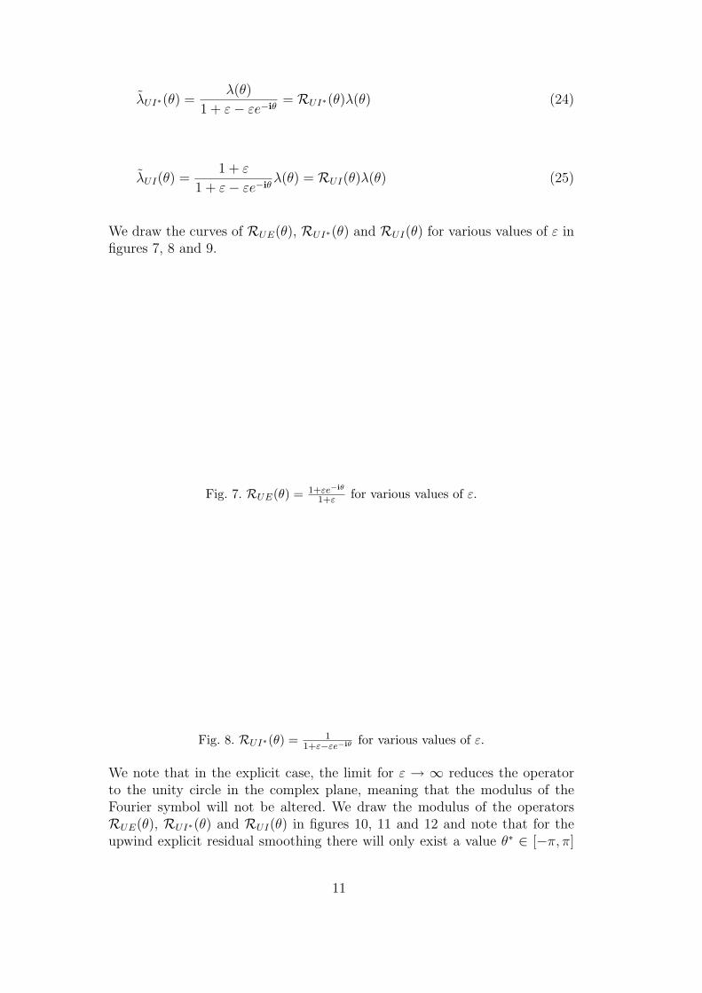
1 + ε− εe−iθ= RUI∗(θ)λ(θ) (24)

λ̃UI(θ) =1 + ε

1 + ε− εe−iθλ(θ) = RUI(θ)λ(θ) (25)

We draw the curves of RUE(θ), RUI∗(θ) and RUI(θ) for various values of ε infigures 7, 8 and 9.

Fig. 7. RUE(θ) = 1+εe−iθ

1+ε for various values of ε.

Fig. 8. RUI∗(θ) = 11+ε−εe−iθ for various values of ε.

We note that in the explicit case, the limit for ε → ∞ reduces the operatorto the unity circle in the complex plane, meaning that the modulus of theFourier symbol will not be altered. We draw the modulus of the operatorsRUE(θ), RUI∗(θ) and RUI(θ) in figures 10, 11 and 12 and note that for theupwind explicit residual smoothing there will only exist a value θ∗ ∈ [−π, π]

11

Fig. 9. RUI(θ) = 1+ε1+ε−εe−iθ for various values of ε.

Fig. 10. Modulus of RUE(θ) = 1+εe−iθ

1+ε for various values of ε.

Fig. 11. Modulus of RUI∗(θ) = 11+ε−εe−iθ for various values of ε.

such that λ̃UE(θ∗) = 0 with λ(θ∗) 6= 0 when ε = ±1. UIRS does not contain

12

Fig. 12. Modulus of RUI(θ) = 1+ε1+ε−εe−iθ for various values of ε.

this singularity except at θ = 0 in the limit ε →∞ and for ε = −1.

We show what happens to the Fourier symbol under the effect of smoothing,for which we again use the U1 discretization with ∆x = 1 as an example(figures 13, 14,and 15).

Fig. 13. λ̃UE(θ) for U1. Various values of ε; bold line represents high frequencymodes.

Both the implicit formulations give similar results, apart from the re-scaling,which makes their effect more apparent. At first sight it appears that theshape of the Fourier symbol does not change, but this is deceptive, as the mainalteration is the clustering of high frequency Fourier modes (the boldest line inthe figures). This clustering is not present in the explicit upwind formulation.It is also apparent that the clustering in UIRS is more pronounced than inCIRS. In the limit for ε → ∞, λ̃UI(θ) will even be reduced to a single point1 + 0i, apart from the singularity at the point for which θ = 0 (λ(0) = 0). Wewill discuss this further below.

13

Fig. 14. λ̃UI∗(θ) for U1. Various values of ε; bold line represents high frequencymodes.

Fig. 15. λ̃UI(θ) for U1. Various values of ε; bold line represents high frequencymodes.

4.3 Further discussion about upwind implicit residual smoothing

We saw in the previous paragraph that UIRS would allow us to obtain extremeclustering of the high frequency modes of the U1 scheme for ε → ∞. This ishardly surprising, as the smoothing operator in that case reduces to

r̃j − r̃j−1 = rj (26)

Solving this implicit equation would imply computing the inverse of a matrixwhich is exactly the discretization operator of the U1 scheme. In other words,we would be preconditioning the scheme with A−1. This would incur the samecost as solving the model problem. For that reason we have dropped the use ofUIRS on the U1 discretization in section 5, after it had been verified that the

14

optimization procedure indeed led to the optimal value ε ≈ ∞. Neverthelessthis discussion clearly shows whence the performance of UIRS originates andhow it can be successfully employed on more complex problems like the Eulerequations, if the latter have been preconditioned such that its Fourier footprintclosely matches that of (17). As in most cases implicit smoothing is doneby using a sequence of Jacobi iterations (effectively creating an approximateinverse of the smoothing operator), it would be necessary to investigate whichwould be the optimal way to do so.We get markedly different effects on the U2 and K3 discretizations (figures 16and 17). The clustering of the high frequency modes is no longer discernableand, strangely, from ε = 1 onwards the smoothed Fourier symbol for K3starts to ”fold back” on itself, meaning that some points in the complex planecorrespond to two different frequencies (figure 17). This lack of clusteringleads us to believe that the current formulation of UIRS is only well suited forfirst order upwind discretizations and that the use of a higher order residualsmoother might improve the results for higher order discretizations.

Fig. 16. λ̃UI(θ) for U2. Various values of ε; bold line represents high frequencymodes.

Remarks :It might seem counter-intuitive to use negative smoothing factors (ε), but itcan be easily seen from the mathematical expression in (25) that apart fromε ∈ [−1, 0[ these are perfectly acceptable, although we have to note that forlarge values of ε we would get about the same result for ε as for −ε.

Something that is less obvious in figures 16 and 17 is how fast the Fouriersymbol ”travels” along its curve. By that we mean that, even for small valuesof θ, λ̃UI(θ) will already be a respectable distance from the origin, which - aswill become clear in section 5 - greatly improves the convergence performanceas the modes for which λ(θ) ≈ 0 are the hardest to smooth.

The above discussion about the effect of UIRS on the U1 discretization would

15

Fig. 17. λ̃UI(θ) for K3. Various values of ε; bold line represents high frequencymodes.

carry over to CIRS with ε →∞ used on the Poisson equation, indicating thatit is a very good choice for elliptic problems.

5 Optimization of parameters

5.1 Objective function

5.1.1 Objective function without residual smoothing

When using the Fourier representation of the discretization scheme, we canassociate an eigenvalue λ(θ) with every θ ∈ [−π, π]. We decompose the er-ror vector with respect to the corresponding eigenvectors. Equation (5) thenbecomes

(en+1)θ = Pm(−λ(θ))(en)θ (27)

16

The eigenvector corresponding to the eigenvalue 0 is the ”constant vector”(= [1 1 . . . 1]T ), which we assume to be eliminated due to the presence ofboundary conditions.While it is possible to find coefficients that allow equation (13) to be solvedwith (2) it will always suffer from very slow convergence, as for values of θfor which λ(θ) ≈ 0 we will have Pm(−λ(θ)) ≈ 1. For that reason multi-gridschemes are used, in which (2) serves as a smoother.We recall that there are two ways to define ”smooth” errors. In geometricalmulti-grid, these are the errors that vary slowly over the grid, i.e. those withθ ∈ ΦLF = [−π

2, π

2]. In an algebraic multi-grid, ”smooth” denotes the errors

that cannot easily be reduced by the smoother, i.e. those with λ(θ) ≈ 0. In thispaper we will limit ourselves to geometrical multi-grid, as for the equationsunder consideration both approaches are similar.When looking for good coefficients we want a scheme that adequately reduceserrors for which θ ∈ ΦHF = [−π, π] \ ΦLF . We define the smoothing factorρHF as

ρHF = supθ∈ΦHF

|Pm(−λ(θ))| (28)

Most previous studies (e.g. [2,9]) tried to find the lowest smoothing factor,ignoring the effect of the remainder of the multi-grid cycle. We previouslyfound [4] that an integrated approach, taking the effect of all components ofa 2-grid cycle into account gave better results, which corresponded well withthe convergence recorded on actual solvers. We assumed that the solution onthe coarser grid (defect correction) is exact (ideal two-grid cycle). This couldbe done by a direct solver or an indirect solver, so that this approach couldrepresent a V,W or F multi-grid cycle depending on how the defect correc-tion is actually computed. Solving the coarse grid equation exactly does notnecessarily mean that all errors corresponding to θ ∈ ΦLF will be completelyannihilated, as due to the restriction and prolongation process (which act asnon-ideal low-pass filters) some high frequencies will be passed to the coarsegrid (aliasing), while the low frequencies will be attenuated. We will only quan-tify the latter effect, ignoring aliasing. We use full weighting for the restrictionand linear interpolation for the prolongation. The proposed objective function(depending on the iteration coefficients) is then

I = supθ∈[−π,π]

|µ(λ(θ))| (29)

where

17

µ(λ(θ)) = D(λ(θ))(Pm(−λ(θ))

)2for θ ∈ ΦLF (30)

(Pm(−λ(θ)))2 for θ ∈ ΦHF (31)

where

D(λ(θ)) =

1−(

cosθ

2

)42λ(θ)

λ(2θ)

(32)

(Pm(−λ(θ)))2 models the effect of pre- and post-smoothing; D(λ(θ)) the de-

fect correction on the coarser grid;(cos θ

2

)4is the combined filtering effect of

restriction and prolongation; 2λ(θ)λ(2θ)

takes into account the discrepancy due to

the truncation error between the matrices on the fine and coarse grid. (Formore details see [4].)Note that the minimization procedure will automatically satisfy the stabilityconstraint I ≤ 1.As we have shown in [4], the objective functions (29) will generally resultin multi-stage schemes that are not as good as smoothers, but give a bet-ter overall performance after one complete V-cycle. Also, the correlation withmeasured convergence rates of two-grid V-cycles was very good.

5.1.2 Objective function with residual smoothing

For the cases when we use CERS, CIRS, UERS or UIRS we use similar ex-pressions as (29)-(32), but distinguish three subcases for each

(1) Residual smoothing in the Runge-Kutta smoother meaning that we re-place λ(θ) by λ̃(θ) in equation (30),(31) in Pm(−λ(θ)) but not in D(λ(θ)).We will call these optimizers ICERS,RK etc. (see §3.1).

(2) Residual smoothing as a filter applied just prior the restriction to thecoarser grid, meaning that we replace equation (32) by

D̃(λ(θ)) =

1−R(θ)

(cos

θ

2

)42λ(θ)

λ(2θ)

(33)

where R, can be either RCE,RCI ,RUE orRCI . We will call these optimiz-ers ICERS,fil etc. (see §3.2).

(3) Residual smoothing as a preconditioner of the original equations: theFourier symbol is altered by residual smoothing everywhere, meaningthat we replace λ(θ) in equation (30), (31) and (32) everywhere by itssmoothed counterpart (including the coarser grid). This has the same

18

effect as using a different discretization scheme from the start. We willcall these optimizers ICERS,all etc. We include these for comparison only.(see §3.3).

For the implicit cases we use the formulations of equations (10) and (11) wasused as the original formulation in (7) and (9) lead to rounding errors due tothe fact that combinations occurred of very high values of ε (small values ofλ(θ)) and very high iteration coefficients (linked to CFL).

5.2 Optimization approach

To find the optimal parameters for the different objective functions a routinewas written in Matlab 7 that creates a large number of random seed vectors,containing initial guesses for the various parameters. These are then fed toanother routine that computes the value of the chosen objective function forthese seed vectors and starts an optimization procedure based on the Nelder-Mead simplex method that is implemented in Matlab’s fminsearch function.

All schemes under consideration tacitly assume ∆x = 1. If different values of∆x are needed, the following re-scaling can be used

γk → (∆x)kγk (34)

We will compare our results against the optimal coefficients for the U1,U2 andK3 scheme, when optimized for ρHF without residual smoothing. These aretaken from [9] and can be found in tables A.1, A.2 and A.3 in appendix A. Itwas found that in these cases the frequencies that converged most slowly werethose around θ = π

2as discussed in [4].

To validate the results obtained by the model (equations (30) and (31)) anactual solver using 2000 nodes was used and its asymptotic convergence ratemeasured in the L2-norm. As in previous studies, the agreement between thisvalue and I was in general very good, thus proving that the latter serves as anadequate model. To be able to compare the merit of schemes with a differentnumber of stages in the R-K iteration, an average convergence factor per stagewas used.

We see that for the values obtained by optimization of ρHF without residualsmoothing a higher number of stages results in a net benefit in the averagesmoothing factor m

√ρHF . For that reason a high number of stages has been

advocated in the past. However, in [4] we showed that this is not the casewhen looking at the complete picture ( 2m

√I). Our conclusion was that a lower

number of stages gave more optimal results when optimizing for I without

19

residual smoothing. For the three schemes these can be summarized as

• U1: m = 2, (γ1, . . . , γm) = (1.0000, 0.3741), 2m√I = 0.7046

• U2: m = 2, (γ1, . . . , γm) = (0.3881, 0.0803), 2m√I = 0.8557

• K3: m = 3, (γ1, . . . , γm) = (1.0537, 0.7632, 0.2417), 2m√I = 0.7861

More details can be found in appendix A (tables A.4, A.5 and A.6).We draw the attention to the fact that the use of a low number of stages issolely based on observation of the scalar advection equation. Transferabilityof this conclusion to the Euler equations still has to be examined.

5.3 Results and discussion

We will use averaged values of the optimization function ( 2m√I) that takes

into account the computational effort of using m stages in both pre- andpost-smoothing. When explicit residual smoothing is used within the Runge-Kutta iteration this effectively doubles the cost per stage; for that reason wealso give the value 4m

√I for info. Explicit residual smoothing only adds one

matrix-vector operation, in which instance 1+2m√I is also given in the tables.

When residual smoothing is used as a preconditioner to the discretized equa-tion we assume the preconditioned matrix is stored and invokes no extra costwithin the iterations. For implicit residual smoothing, the cost is not quanti-fied as it will depend on the way the implicit equation for the smoothing isactually solved.For the U1,U2 and K3 discretizations the optimal results when using centralresidual smoothing can be found in tables 1, 2 and 3, while for the upwindresidual smoothing they are summarized in tables 4, 5 and 6. We recall from§4.3 that the optimal implicit upwind residual smoothing for the U1 discretiza-tion would happen for ε = ∞.

From these results it immediately becomes clear that upwind residual smooth-ing is a far better choice for advection equations. This is very logical as theresulting preconditioning resembles the inverse of A better than for centralresidual smoothing.It is also clear that UIRS has a higher potential than UERS; their respec-tive true gains will depend on the cost of the actual implementation. For theexplicit residual smoothing the improvements are drastically reduced whencounting the cost, to the point that only for U2 there will remain a net bene-fit. It is quite possible that the same happens for implicit residual smoothing,although some basic arithmetic shows that for the U2 discretization with UIRSapplied to the Runga-Kutta iteration a real gain is obtained as long as thetotal cost remains below the equivalent of 31 matrix-vector products.The reason that most is gained in the U2 scheme is probably due to the fact

20

that for U2 the high frequencies are the most spread out and hence benefitmost from the clustering effect of preconditioning.Remarkably, the performance of CERS and CIRS are very similar, while thelatter bears a much higher computational cost.Also, when one has to chose from the three possibilities to apply residualsmoothing it seems the best approach would be to use it only within theRunge-Kutta iteration, while the least can be gained from using it as a filter.

We add that the values of I were compared with convergence factors on actualsolvers and differed by less than 5%.

We illustrate the results for the optimal solution for ”CERS,RK”, ”CIRS,RK”,”UERS,RK” and ”UIRS,RK” for the U2 scheme (figures 18, 19, 20 and 21 .We draw the stability region S = {z ∈ C; |Pm(z)| ≤ 1} on which we super-pose (−λ̃(θ)) and also give |Pm(λ̃(θ))| (the amplification of the smoother) and|µ(λ(θ))| (the amplification of the V-cycle).

From these figures it is easy to see that the main improvement in convergencestems from the clustering of the high frequencies and the altered shape of theFourier symbol that follows the contours of the amplification function better.

6 Conclusions

Central and upwind residual smoothing have been tested on various discretiza-tions of the simple scalar advection equation: U1, U2 and K3. Both explicitand implicit formulations were looked at. These were applied within a multi-grid framework either to the smoother (a multi-stage Runge-Kutta solver),as a filter before the restriction to a coarser grid or as a preconditioner tothe discretized equations. A new optimization function that better resemblesthe real convergence speed was used to find the optimal coefficients for theRunga-Kutta smoother in this context.The best improvements were obtained with upwind implicit schemes, althoughone has to take into account their relative high cost. The most was gained incase the U2 discretization was used.While this simple equation might lead us to a conclusion of excellent conver-gence, it is not so much the result as it is the reason for the improvement thatwe would like to emphasis. Often a reduction in magnitude (modulus) of thehigh frequency modes or the possibility of high CFL numbers has been themain argument. We have pointed out that the former can even be detrimentalwhen used in the smoother as it would bring them closer to the origin, wherethey are difficult to damp. We have shown, that the dominating accelerationmechanisms of residual smoothing are

21

Fig. 18. First figure: Stability region and Fourier symbol (locus of high frequenciesin bold). Second figure: amplification curves |Pm(λ̃(θ))| (dotted line) and |µ(λ(θ))|(solid line) for the optimal U2 scheme with explicit central residual smoothing(CERS,RK). See table 2 for details.

(1) a very rapid progression of λ̃(θ) away from the origin(2) a clustering of the high frequency modes(3) a modification of the shape of the Fourier symbol to better follow the

contours of the transmittance function of the multi-stage smoother.

For the scalar equation the cost of implicit residual smoothing is of the sameorder as the solution of the original problem and thus prohibitive unless anapproximate solution to the residual smoothing equation is used. It is believedhowever that qualitative aspects of this study will carry over to more com-plex problems like the Euler equations if these are preconditioned to closelyfollow the contours of the Fourier symbol of the advection equation. In thoseapplications, the improvement obtained by residual smoothing will outweighits computational cost.

22

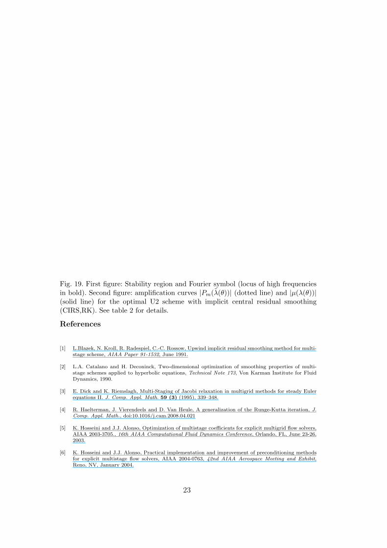
Fig. 19. First figure: Stability region and Fourier symbol (locus of high frequenciesin bold). Second figure: amplification curves |Pm(λ̃(θ))| (dotted line) and |µ(λ(θ))|(solid line) for the optimal U2 scheme with implicit central residual smoothing(CIRS,RK). See table 2 for details.

References

[1] L.Blazek, N. Kroll, R. Radespiel, C.-C. Rossow, Upwind implicit residual smoothing method for multi-stage scheme, AIAA Paper 91-1532, June 1991.

[2] L.A. Catalano and H. Deconinck, Two-dimensional optimization of smoothing properties of multi-stage schemes applied to hyperbolic equations, Technical Note 173, Von Karman Institute for FluidDynamics, 1990.

[3] E. Dick and K. Riemslagh, Multi-Staging of Jacobi relaxation in multigrid methods for steady Eulerequations II. J. Comp. Appl. Math. 59 (3) (1995), 339–348.

[4] R. Haelterman, J. Vierendeels and D. Van Heule, A generalization of the Runge-Kutta iteration, J.Comp. Appl. Math., doi:10.1016/j.cam.2008.04.021

[5] K. Hosseini and J.J. Alonso, Optimization of multistage coefficients for explicit multigrid flow solvers,AIAA 2003-3705., 16th AIAA Computational Fluid Dynamics Conference, Orlando, FL, June 23-26,2003.

[6] K. Hosseini and J.J. Alonso, Practical implementation and improvement of preconditioning methodsfor explicit multistage flow solvers, AIAA 2004-0763, 42nd AIAA Aerospace Meeting and Exhibit,Reno, NV, January 2004.

23

Fig. 20. First figure: Stability region and Fourier symbol (locus of high frequenciesin bold). Second figure: amplification curves |Pm(λ̃(θ))| (dotted line) and |µ(λ(θ))|(solid line) for the optimal U2 scheme with explicit upwind residual smoothing(UERS,RK). See table 5 for details.

[7] K. Hosseini, Practical implementation of robust preconditioners for optimized multistage flow solvers,Ph.D. thesis, Stanford University, 2005.

[8] J.F. Lynn, Multigrid solution of the Euler equations with local preconditioning, Ph.D. Thesis, TheUniversity of Michigan, 1995

[9] B. Van Leer, C.H. Tai and K.G. Powell, Design of optimally smoothing multi-stage schemes for theEuler Equations, AIAA Paper 89-1923 (1989).

[10] Z.W. Zhu, C.Lacor, C. Hirsch, A new residual smoothing method for multigrid multi-stage schemes,in: Proc. of the 11th AIAA CFD Conference, AIAA-93-3356-CP, 1993.

A Optimal coefficients from previous studies

The results below are taken from [9], resp. [4], and give the optimal coefficientsfor the optimzer ρHF , resp. (29), without the use of residual smoothing. IE

is the convergence factor measured on an actual solver over a V-cycle. It can

24

be seen that this closely matches values of I, validating our model, exceptfor very low values of m when aliasing (which our model ignores) was tooimportant.

25

Optimizer Optimizer m (γ1, . . . , γm) ε

2m√ICERS,RK = 0.6586 4m

√ICERS,RK = 0.8115 2 (1.8255 , 1.4712) 0.2632

2m√ICIRS,RK = 0.6586 2 (0.8996 , 0.3573) 0.7155

2m√ICERS,all = 0.6596 2 (1.7482 , 1.3477) 0.2444

2m√ICIRS,all = 0.6735 2 (0.9928 , 0.4140) 0.2107

2m√ICERS,fil = 0.6955 (1+2m)

√ICERS,fil = 0.7479 2 (1.0000 , 0.3709) -0.1822

2m√ICIRS,fil = 0.6955 2 (1.0000 , 0.3709) 0.1107

Table 1Advection equation using U1. Optimal coefficients for Runge-Kutta with centralresidual smoothing.

Optimizer Optimizer m (γ1, . . . , γm) ε

2m√ICERS,RK = 0.7914 4m

√ICERS,RK = 0.9293 3 (1.4224 , 1.3753 , 0.5854) 0.3602

2m√ICIRS,RK = 0.7699 3 (0.5841 , 0.2187 , 0.0415) 3.1230

2m√ICERS,all = 0.7630 3 (1.4586 , 1.3324 , 0.5574) 0.3526

2m√ICIRS,all = 0.7732 3 (0.6613 , 0.2848 , 0.0541) 0.9618

2m√ICERS,fil = 0.8331 (1+2m)

√ICERS,fil = 0.8641 2 (0.4000 , 0.0809) -0.2749

2m√ICIRS,fil = 0.8463 2 (0.3960 , 0.0813) 0.2565

Table 2Advection equation using U2. Optimal coefficients for Runge-Kutta with centralresidual smoothing.

Optimizer Optimizer m (γ1, . . . , γm) ε

2m√ICERS,RK = 0.7603 4m

√ICERS,RK = 0.8720 4 (2.2450 , 3.0512 , 2.5146 , 1.0678) 0.1771

2m√ICIRS,RK = 0.7561 4 (1.5830 , 1.5095 , 0.8719 , 0.2663) 0.3263

2m√ICERS,all = 0.7603 4 (2.1231 , 2.7389 , 2.1224 , 0.8486) 0.1516

2m√ICIRS,all = 0.7562 4 (1.5711 , 1.5088 , 0.8693 , 0.2596) 0.2382

2m√ICERS,fil = 0.7823 (1+2m)

√ICERS,fil = 0.8039 4 (1.4008 , 1.3132 , 0.6865 , 0.1693) -0.1568

2m√ICIRS,fil = 0.7847 4 (1.3989 , 1.3183 , 0.6894 , 0.1692) 0.0710

Table 3Advection equation using K3. Optimal coefficients for Runge-Kutta with centralresidual smoothing.

Optimizer Optimizer m (γ1, . . . , γm) ε

2m√IUERS,RK = 0.4965 4m

√IUERS,RK = 0.7046 1 (1.0000) 0.5978

2m√IUERS,all = 0.5836 1 (0.6653) 0.1888

2m√IUERS,fil = 0.6549 (1+2m)

√IUERS,fil = 0.7127 2 (1.0000 , 0.3572) 0.9903

2m√IUIRS,fil = 0.6563 2 (1.0000 , 0.3577) 0.1776

Table 4Advection equation using U1. Optimal coefficients for Runge-Kutta with explicitupwind residual smoothing.

26

Optimizer Optimizer m (γ1, . . . , γm) ε

2m√IUERS,RK = 0.7108 4m

√IUERS,RK = 0.8431 2 (1.1507 , 0.5169) 0.7458

2m√IUIRS,RK = 0.2538 2 (1.3107 , 0.4317) -9.4865

2m√IUERS,all = 0.7505 2 (1.0686 , 0.4887) 0.7605

2m√IUIRS,all = 0.3296 2 (1.3299 , 0.4418) -162.0642

2m√IUERS,fil = 0.8288 (1+2m)

√IUERS,fil = 0.8605 2 (0.3846 , 0.0766) 2.1779

2m√IUIRS,fil = 0.8165 2 (0.4032 , 0.0800) 0.4444

Table 5Advection equation using U2. Optimal coefficients for Runge-Kutta with upwindresidual smoothing.

Optimizer Optimizer m (γ1, . . . , γm) ε

2m√IUERS,RK = 0.6812 4m

√IUERS,RK = 0.8254 3 (2.2311 , 2.4489 , 1.2241) 0.4230

2m√IUIRS,RK = 0.3750 4 (4.2684 , 7.1418 , 5.5676 , 1.7262 ) 453.6564

2m√IUERS,all = 0.7094 3 (1.9347 , 2.1126 , 0.9620 ) 0.3214

2m√IUIRS,all = 0.4136 2 (2.0331 , 1.1846) 1.167 · 1013

2m√IUERS,fil = 0.7620 (1+2m)

√IUERS,fil = 0.7921 3 (1.0947 , 0.7717 , 0.2359) 0.6260

2m√IUIRS,fil = 0.7692 3 (1.0644 , 0.7387 , 0.2313) 0.2040

Table 6Advection equation using K3. Optimal coefficients for Runge-Kutta with upwindresidual smoothing.

m =1 m =2 m =3 m =4 m =5 m =6

γ1 0.5000 1.0000 1.5000 2.0000 2.5000 3.0000

γ2 0.3333 0.9000 1.7060 2.7588 4.0608

γ3 0.2000 0.7059 1.6380 3.1211

γ4 0.1176 0.5172 1.4242

γ5 0.0689 0.3636

γ6 0.0404

m√

ρHF 0.7078 0.5786 0.5226 0.4941 0.4780 0.4785

2m√I 0.7056 0.7159 0.7703 0.8071 0.8329 0.8521

2m√IE 0.6267 0.7171 0.7702 0.8075 0.8333 0.8525

Table A.1Advection equation using U1: optimal m-stage coefficients for ρHF after conversionfrom [9] to the formulation in (2).

27

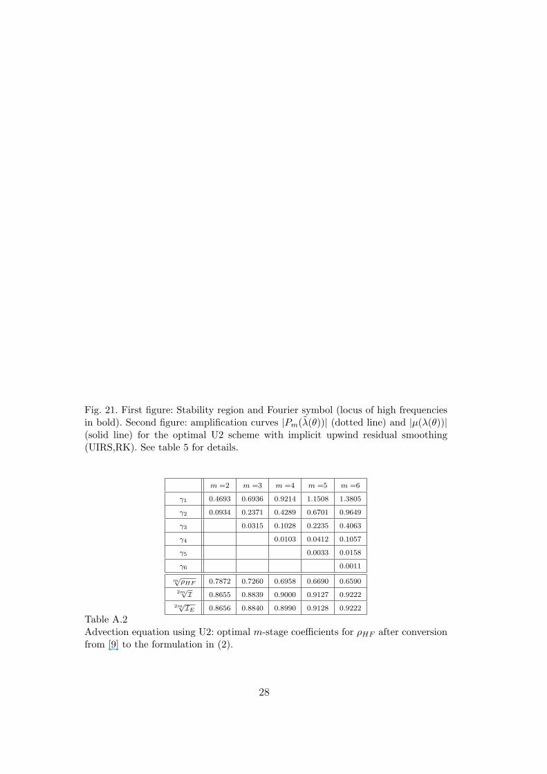
Fig. 21. First figure: Stability region and Fourier symbol (locus of high frequenciesin bold). Second figure: amplification curves |Pm(λ̃(θ))| (dotted line) and |µ(λ(θ))|(solid line) for the optimal U2 scheme with implicit upwind residual smoothing(UIRS,RK). See table 5 for details.

m =2 m =3 m =4 m =5 m =6

γ1 0.4693 0.6936 0.9214 1.1508 1.3805

γ2 0.0934 0.2371 0.4289 0.6701 0.9649

γ3 0.0315 0.1028 0.2235 0.4063

γ4 0.0103 0.0412 0.1057

γ5 0.0033 0.0158

γ6 0.0011

m√

ρHF 0.7872 0.7260 0.6958 0.6690 0.6590

2m√I 0.8655 0.8839 0.9000 0.9127 0.9222

2m√IE 0.8656 0.8840 0.8990 0.9128 0.9222

Table A.2Advection equation using U2: optimal m-stage coefficients for ρHF after conversionfrom [9] to the formulation in (2).

28

m =2 m =3 m =4 m =5 m =6

γ1 0.8276 1.3254 1.7320 2.1668 2.5975

γ2 0.4535 0.8801 1.5824 2.4419 3.4956

γ3 0.3364 0.8296 1.7101 2.9982

γ4 0.2394 0.7333 1.7118

γ5 0.1695 0.6194

γ6 0.1194

m√

ρHF 0.8383 0.7769 0.7385 0.7150 0.7018

2m√I 0.8491 0.8426 0.8531 0.8668 0.8788

2m√IE 0.8585 0.8423 0.8575 0.8646 0.8786

Table A.3Advection equation using K3: optimal m-stage coefficients for ρHF after conversionfrom [9] to the formulation in (2).

m =1 m =2 m =3 m =4 m =5 m =6

γ1 0.5000 1.0000 1.5000 1.9951 2.4560 2.8638

γ2 0.3741 1.1043 2.1789 3.5724 5.1645

γ3 0.3021 1.1811 2.9506 5.4415

γ4 0.2557 1.2980 3.3859

γ5 0.2357 1.1624

γ6 0.1708

m√

ρHF 0.7078 0.7046 0.7475 0.7791 0.8032 0.8202

2m√I 0.7056 0.7046 0.7475 0.7790 0.8011 0.8201

2m√IE 0.6267 0.7082 0.7452 0.7798 0.7966 0.8173

Table A.4Advection equation using U1: optimal m-stage coefficients for I. From [4].

m =2 m =3 m =4 m =5 m =6

γ1 0.3881 0.5893 0.7901 0.9863 1.1651

γ2 0.0803 0.2294 0.4414 0.7090 1.0130

γ3 0.0331 0.1230 0.2875 0.5320

γ4 0.0139 0.0630 0.1703

γ5 0.0058 0.0307

γ6 0.0024

m√

ρHF 0.8557 0.8636 0.8721 0.8801 0.8863

2m√I 0.8557 0.8636 0.8721 0.8797 0.8863

2m√IE 0.8555 0.8664 0.8688 0.8800 0.8809

Table A.5Advection equation using U2: optimal m-stage coefficients for I. From [4].

29

m =2 m =3 m =4 m =5 m =6

γ1 0.6499 1.0537 1.3982 1.7255 2.1893

γ2 0.3070 0.7632 1.3316 2.0143 3.1388

γ3 0.2417 0.6985 1.4457 2.9109

γ4 0.1712 0.6372 1.8290

γ5 0.1412 0.7359

γ6 0.1512

m√

ρHF 0.8241 0.7861 0.7894 0.8018 0.8137

2m√I 0.8241 0.7861 0.7894 0.8018 0.8137

2m√IE 0.8692 0.7871 0.7960 0.8005 0.8131

Table A.6Advection equation using K3: optimal m-stage coefficients for I. From [4].

30